Article

Joint Optimization of Carrier Frequency and PRF for Frequency Agile Radar Based on Compressed Sensing

by
Zhaoxiang Yang
1,
Hao Zheng
2,3,*,
Yongliang Zhang
1,
Junkun Yan
4 and
Yang Jiang
1
1
College of Transportation, Inner Mongolia University, Hohhot 010030, China
2
College of Electronic Information Engineering, Inner Mongolia University, Hohhot 010021, China
3
Inner Mongolia Key Laboratory of Intelligent Communication and Sensing and Signal Processing, Inner Mongolia University, Hohhot 010021, China
4
National Key Laboratory of Radar Signal Processing, Xidian University, Xi’an 710071, China
*
Author to whom correspondence should be addressed.
Remote Sens. 2025, 17(10), 1796; https://doi.org/10.3390/rs17101796
Submission received: 15 March 2025 / Revised: 8 May 2025 / Accepted: 18 May 2025 / Published: 21 May 2025

Abstract

:
Frequency agile radar (FAR) exhibits robust anti-jamming capabilities and a superior low probability of intercept performance due to its randomized carrier frequency (CF) and pulse repetition frequency (PRF) hopping sequences. The advent of compressed sensing (CS) theory has effectively addressed the coherent processing challenges of frequency agile signals. Nonetheless, the reconstructed results often suffer from elevated sidelobe levels, which lead to significant sparse recovery errors. The performance of sparse reconstruction is greatly influenced by the correlation between the dictionary matrix columns. Specifically, weaker correlation usually means better target detection performance and lower false alarm probability. Consequently, this paper adopts the maximum coherence coefficient (MCC) between the dictionary matrix columns as the cost function. In addition, in order to reduce the correlation of the dictionary matrix and improve the target detection performance, a genetic algorithm (GA) is employed to jointly optimize the CF hopping coefficients and PRFs of the FAR. The echo of optimized signals is subsequently reconstructed using the alternating direction method of multipliers (ADMM) algorithm. Simulation results demonstrate the effectiveness of the proposal.

1. Introduction

Currently, the mainstream pulse-Doppler radars typically employ waveforms with fixed carrier frequency (CF) and constant pulse repetition frequency (PRF) within a coherent processing interval (CPI) [1,2]. However, such fixed-parameter radar signals are susceptible to interception and analysis by enemy electronic countermeasures (ECMs). In this context, frequency agile radar (FAR) has emerged. Early-stage FARs were mainly stepped frequency radars, which can achieve a wideband effect under the low hardware system cost [3]. However, the monotonous CF stepping mode allows the jammer to easily predict changes during the pulses, which limits its anti-jamming ability [4]. The current FARs not only generate high-range-resolution profiles but also exhibit excellent anti-jamming and electronic counter-countermeasures (ECCMs) performance, because the randomly varied CF or PRF of the pulses are difficult to track and predict.
Traditional radars employ the classical coherent processing techniques, such as matched filtering, moving target detection (MTD) and moving target indicator (MTI). However, for FAR, owing to the discontinuity of the signal phase caused by the hopping of CF and PRF in a CPI  [3,5], traditional coherent processing techniques are no longer applicable. In 1995, Wehner introduced an extended stretch method based on matched filtering theory, which achieved the coherent processing of CF agile radar. This breakthrough marks the advent of fully coherent CF agile radar systems [6]. However, this extended stretch method leads to the sidelobe pedestal problems [7]. Therefore, weak targets may be masked by the sidelobe of dominant ones. By exploiting target sparsity, compressed sensing (CS) techniques have been applied in order to alleviate the sidelobe pedestal problem [8,9]. To address phase variations in echoes caused by CF agility, the work in [10] applied phase compensation under the minimum waveform entropy criterion as a cost function and achieved coherent processing through fast Fourier transform (FFT). For PRF agile radars, its echo has non-uniform characteristics when sampled between different pulses within the same range bin. Therefore, in [11], adaptive iterative algorithms have been progressively employed to address coherent integration challenges. In [12], in order to resolve the coherent integration issues caused by non-uniform sampling, a hybrid approach integrating Radon transform with non-uniform FFT is proposed.
CS is a novel theory that differs from the traditional Nyquist sampling theorem. The conventional Nyquist sampling theorem states that the sampling rate of a received signal must be at least twice the signal bandwidth. Otherwise, aliasing will occur, which leads to the loss of sampled signal information. In contrast, CS theory posits that a high-dimensional signal, which allows a sparse representation on a suitable basis, can be recovered from highly incomplete linear measurements by using efficient algorithms. This theory has the advantages of a compressed sampling rate and the high-precision reconstruction of data. In radar detection scenarios, the detected targets are usually sparse. Therefore, CS models are naturally suitable for radar signal processing  [13]. The reconstruction algorithms for the CS model mainly include the convex-optimization algorithm and greedy algorithm. For convex optimization, it mainly contains basis pursuit (BP) and the alternating direction method of multipliers (ADMM). And the greedy algorithm primarily consists of matching pursuit (MP), orthogonal matching pursuit (OMP), stagewise orthogonal matching pursuit (StOMP), and regularized orthogonal matching pursuit (ROMP). The work in [14,15,16] effectively addressed the coherent integration challenges of echo signals in FAR by leveraging CS principles. Furthermore, sparse Bayesian learning (SBL) is used in [17] for sparse reconstruction in FAR. Liu Zhen et al. adopted a CS-based signal processing method in [18,19,20], which successfully transformed velocity estimation into a typical CS model and achieved a coherent integration of echo signals.
When processing FAR echo signals through CS, the reconstruction performance is determined by the dictionary matrix, which is related to the CF and PRF hopping sequences. Specifically, the weaker correlation between dictionary matrix columns corresponds to better target detection performance and lower false alarm probability. The work in [21] introduced an improved particle swarm optimization (PSO) to reduce the correlation between columns in the dictionary matrix, but the outcome of the optimization is not significant. When using simulated annealing (SA) to optimize the CF hopping coefficients, its convergence speed for calculating and iterating the dictionary matrix is relatively slow. In this paper, we propose a radar signal model with joint agility in CF and PRF. A dictionary matrix is constructed through CS, and the correlation between dictionary matrix columns is used as the fitness function. Then, a genetic algorithm (GA) is employed to optimize the CF and PRF hopping sequences to reduce the correlation of the dictionary matrix. Finally, the ADMM is utilized to reconstruct the echoes of the optimized sequences. Simulation results demonstrate that the dictionary matrix constructed from the optimized agile radar signals exhibits lower column correlation, which leads to reconstructed results with lower sidelobe levels.
The organization of this paper is as follows. In Section 1, the signal model of CF-PRF jointly agile radar is given. In Section 2, the signal processing method for CF-PRF jointly agile radar is introduced, including the CS model and ADMM algorithm. Section 3 primarily presents the dictionary matrix optimization method based on the GA. Section 4 describes the simulation parameters and simulation results to evaluate the effectiveness of the proposed method. Finally, conclusions are drawn in Section 5.

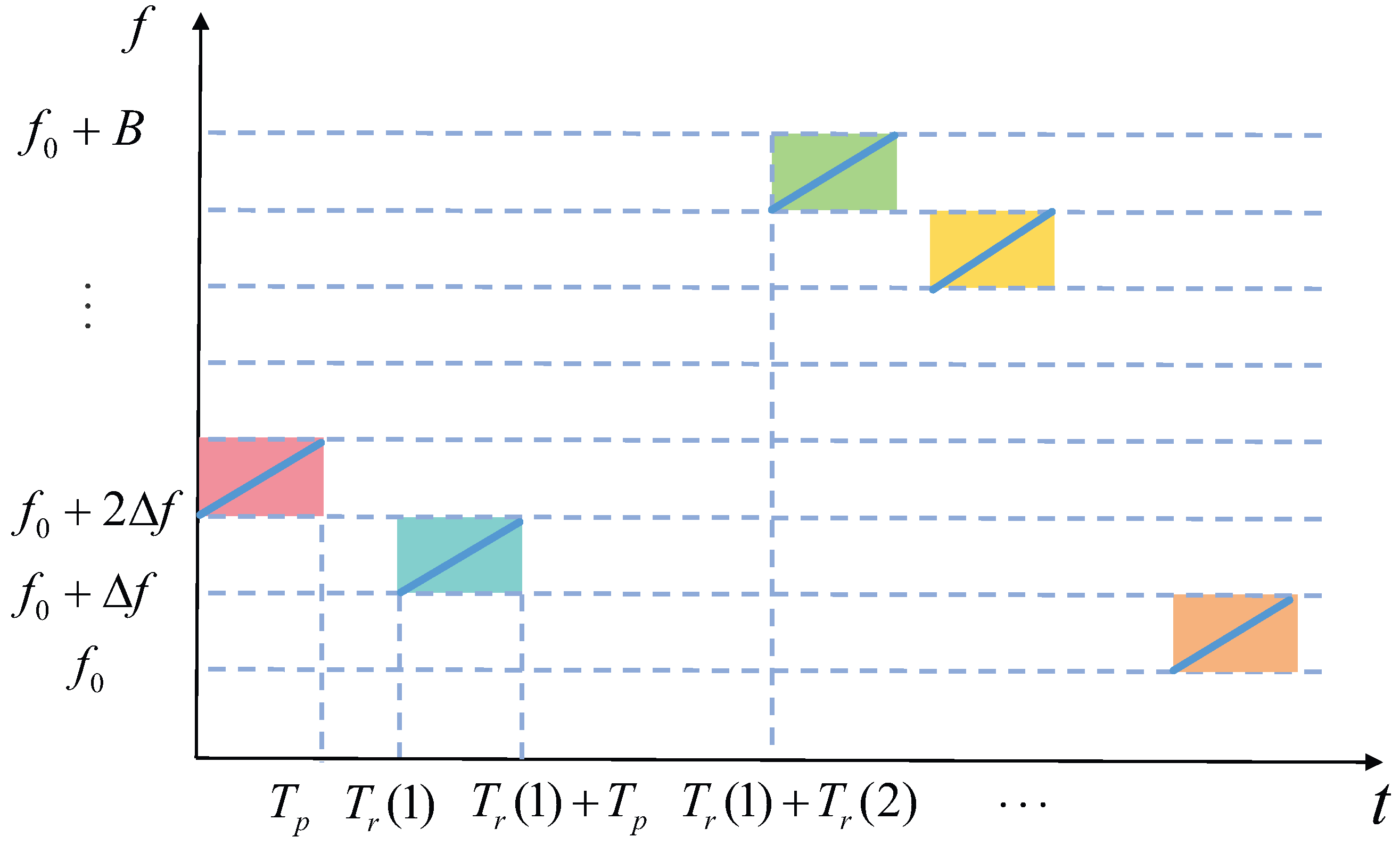
2. CF-PRF Jointly Agile Radar Signal Model

In the design process of the FAR system, in order to meet the requirements of transmit power and range resolution, FAR commonly adopts the linear frequency modulation (LFM) signal as its transmit waveform. For a CF-PRF jointly agile pulse sequence with N pulses, its expression can be expressed as shown below:
S t ( t ) = n = 0 N 1 rect t t n T p e j π μ ( t t n ) 2 e j 2 π f n t
where T p is the pulse width, which is going to be kept constant in this system. μ = B 0 / T p represents the chirp rate, and  B 0 denotes the signal bandwidth and is a constant. f n = f 0 + m ( n ) Δ f is the CF of the n-th pulse, n = 0 , 1 , , N 1 , f 0 stands for the initial CF of the signal, m ( n ) is the CF hopping code sequence and m ( n ) { 0 , 1 , , M 1 } , where M is the number of available CF points. Δ f is the bandwidth of the CF hopping step and we set B 0 = Δ f so that the frequency bands between each pulse do not overlap. The synthetic bandwidth of the radar is B = ( M 1 ) Δ f + B 0 = M Δ f . The pulse repetition interval (PRI) of the n-th pulse T r ( n ) randomly hops within a certain range, which is larger than T p , and  T r ( 0 ) = 0 . T r ( n ) is the inverse of the PRF, indicating that the PRFs of the FAR also randomly hop within a certain range. t n represents the total transmission time of the previous n 1 pulse and t n = i = 0 n 1 T r ( i ) . rect ( ) is the unit rectangular function:
rect ( t t n T p ) = 1 , T p 2 + t n < t < T p 2 + t n 0 , otherwise
For a pulse sequence with randomly varying CF and PRF within a certain range, the variation of the CF and PRF is illustrated in Figure 1.
From Figure 1, it can be observed that the CF of each pulse and the PRF between adjacent pulses hop randomly. Assume that there exists a scatterer moving along the line of sight of the radar at velocity ν and the initial radial distance is R. After reflection from the target, the radar echo signal can be represented as
S r ( t ) = n = 0 N 1 rect ( t t n τ T p ) e j π μ ( t t n τ ) 2 e j 2 π f n ( t τ )
where τ = 2 ( R + ν t n ) / c is the time delay, and c represents the speed of light. After the radar receiver captures the echo signal, the echo signal should be processed by down-conversion with the mixing signal e j 2 π f n t . Then, we perform pulse compression. The resulting signal can be expressed as shown below:
S r ( t ) = n = 0 N 1 β s i n c ( π B 0 ( t τ ) ) e j 2 π f n τ
where β denotes the amplitude of the echo signal after pulse compression. By substituting τ = 2 ( R + ν t n ) / c into Equation (4), we can obtain
S r ( t ) = n = 0 N 1 β s i n c ( π B 0 ( t τ ) ) e j 4 π f n R c e j 4 π f n ν t n c
By substituting f n = f 0 + m ( n ) Δ f into Equation (5), the resulting signal can be expressed as shown below:
S r ( t ) = n = 0 N 1 β s i n c ( π B 0 ( t τ ) ) e j 4 π f 0 R c e j 4 π m ( n ) Δ f R c e j 4 π f 0 ν t n c e j 4 π m ( n ) Δ f ν t n c
From this, we derive the echo signal model of CF and PRF jointly agile radar.

3. CF-PRF Jointly Agile Radar Signal Processing Method

As seen in Equation (6), the phase variation of the received signal is related to the introduced random variables m ( n ) and t n , which leads to the lack of linear characteristics in the echo phase. At this time, the FFT will completely lose effectiveness. Applying traditional coherent processing techniques to CF-PRF jointly agile radar directly leads to a sidelobe pedestal, which may affect the detection of weak targets. The advent of CS has effectively addressed the signal processing challenges in FAR systems.

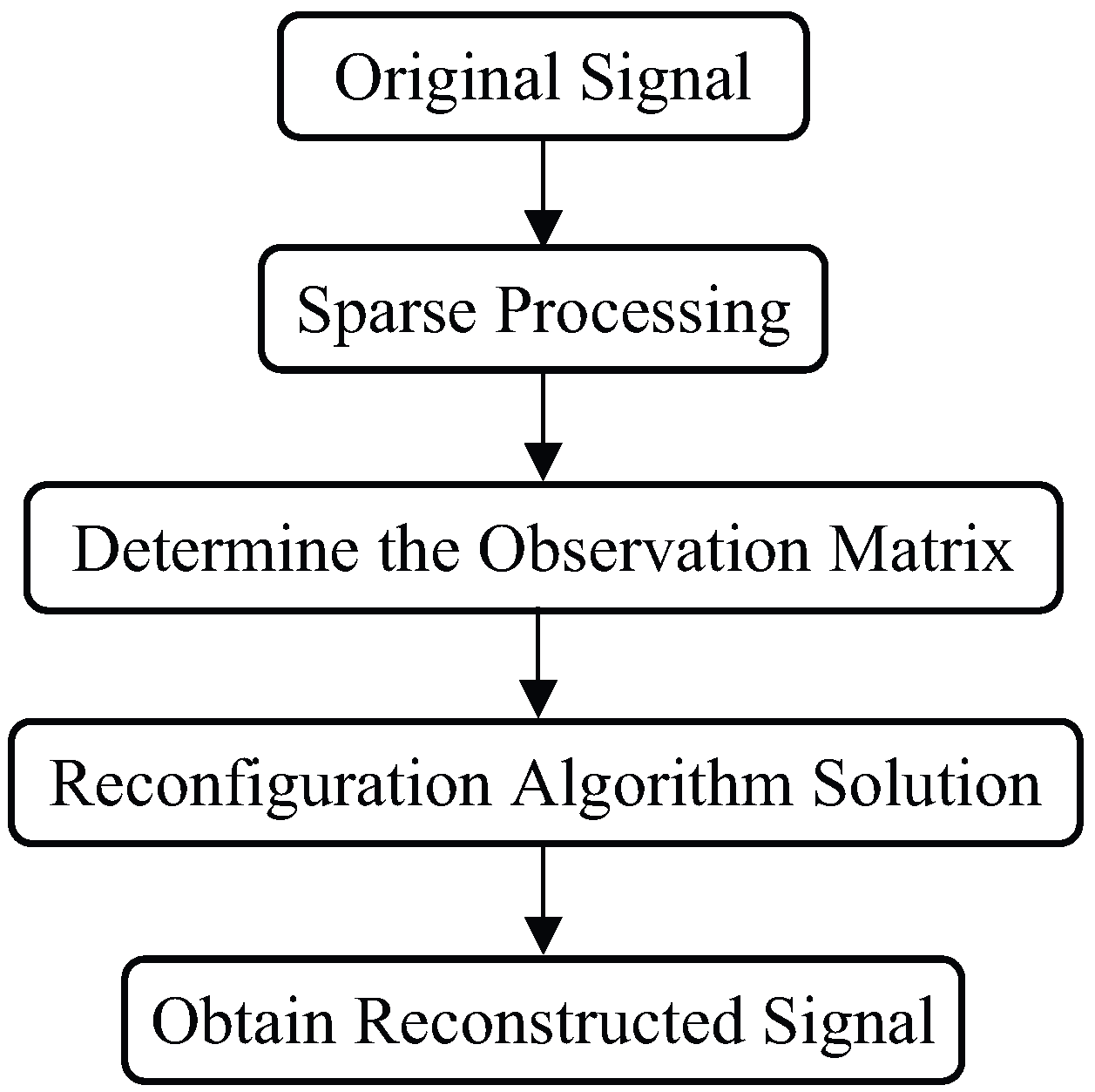
3.1. The Theory Model of CS

The main process of CS is shown in Figure 2.
Define an S-dimensional signal x x C S . Φ = ϕ 1 , ϕ 2 , , ϕ S is defined as a set of orthogonal basis vectors in the C S space. The signal x can be represented by Φ .
Define an S-dimensional recovery vector θ = θ 1 , θ 2 , , θ S . θ i = x , ϕ i = ϕ i H x , where H is the complex conjugate-transpose operator, and notation a , b is used for the inner product of vectors a and b . And the sparsity K is defined as the number of non-zero elements in vector θ . Therefore, the signal x can be represented using Φ and θ as follows:
x = Φ θ
Now, define an observation matrix A with dimension D × S , where D < S . The observation vector y is obtained by observing the original signal x through A . In the case of D l o g ( S / D ) K , we can recover the original signal x through the observation vector y [22]. Then, y satisfies the following relationship:
y = A x = A Φ θ = Ψ θ
By observing Equation (8), it can be found that the number of equations is naturally less than the number of unknown parameters in θ . In this case, the dictionary matrix Ψ is column-rank deficient, which means that Equation (8) about θ is an under-determined problem. CS is an effective tool for solving such under-determined problem. Because of the sparseness of the observed scene, Equation (8) about θ is converted into a constrained optimization problem about θ , which enables accurate recovery of the original signal θ from the observed measurements y . Under noise-free conditions, the recovery model can be formulated as shown below:
min θ θ 0 subject to ( s . t . ) y = Ψ θ
where · 0 denotes the l 0 norm of a vector.

3.2. CS Model for CF-PRF Jointly Agile Radar Signal Processing

To apply CS to the coherent processing of CF-PRF jointly agile radar, the first step is to convert the echo signal into a sparse representation. Without loss of generality, we focus on a specific range unit and assume that the scatterer is moving inside the unit during the CPI. After down-conversion, for a CF-PRF jointly agile pulse sequence with N pulses, the echo of the n-th pulse can be expressed as shown below:
R x n = σ n e j 4 π f 0 R c e j 4 π Δ f R c m ( n ) e j 4 π f o ν t n c l n
where l n = 1 + m ( n ) Δ f / f 0 represents the relative frequency shift of the n-th pulse with respect to the initial CF f 0 . σ n denotes the back-scattering coefficient. R and ν represent the distance and velocity of the target, respectively. To further simplify the formula, the following new variables are introduced:
γ = σ n e j 4 π f 0 R c p = 4 π Δ f R c q = 4 π f o ν t n c
where γ , p and q are proportional to σ n , R and ν , respectively. γ , p and q are simply called the scattering intensity, range term and Doppler term, respectively. When there are multiple targets with different high-resolution ranges and velocities, i.e., different ( p , q ) parameters, in the observed scene, returns are cast as a superposition of echoes from all targets.
To build the dictionary matrix, we can divide the observation scene into P high-resolution range and Q velocity units. That means the p domain and q domain are divided into P and Q grid points. For tracking radar, the range resolution and the velocity resolution are
Δ r = c 2 B = c 2 M Δ f
Δ ν = c 2 f 0 T
where T = i = 0 N 1 T r ( i ) denotes the total transmission time of N pulses within a CPI. At this point, we can obtain the return of the n-th pulse as
R x ( n ) = i = 0 P 1 k = 0 Q 1 γ i k e j p i m ( n ) + j q k l n
where p i = 4 π Δ f R i c , q k = 4 π f o ν k t n c , respectively, i = 0 , 1 , , P 1 , k = 0 , 1 , , Q 1 . And  R i = r 0 + i Δ r , ν k = k Δ ν , where r 0 represents the starting distance of the range unit. γ i k is the scattering intensity of the target presented at ( p i , q k ) . The primary objective of CS is to reconstruct the target signal from echoes by estimating the scattering intensity γ i k on the high-resolution range-Doppler plane. All possible scenarios can be represented by matrix Γ = [ γ i k ] C P × Q . Each element of this matrix corresponds to the scattering intensity of a specific scenario. Vectorize the intensity matrix Γ into θ C P Q with the l-th element θ l = γ i k ,   l = i + P k = 0 , 1 , , P Q 1 . Then, Equation (14) can be rewritten as shown below:
R x ( n ) = i = 0 P 1 k = 0 Q 1 θ l e j p i m ( n ) + j q k l n
In radar observation scenarios, the number of targets is often small, which leads to most elements of θ corresponding to zero scattering coefficients. In this case, CS can be employed to solve for the target parameters. Define the vector ψ l C N . The  n-th element of ψ l represents the phase relationship of the l-th column of the dictionary matrix for the n-th pulse, and we have
ψ l ( n ) = e j p i m ( n ) + j q k l n
Then, we can rewrite Equation (15) into matrix form:
y = Ψ θ
where y = R x 0 , R x 1 , , R x N 1 T C N is the observation vector, and the dictionary matrix is Ψ = ψ 0 , ψ 1 , , ψ P Q 1 , Ψ C N × P Q .
Based on the above derivation, when the radar parameters are known, a dictionary matrix can be constructed according to the following equation:
Ψ ( n , l ) = exp j 4 π m n Δ f R i c exp j 4 π f 0 ν k t n c 1 + m n Δ f f 0
where n = 0 , 1 , , N 1 and l = i + P k = 0 , 1 , , P Q 1 .

3.3. CF-PRF Jointly Agile Radar Signal Processing Method Based on ADMM

As an efficient distributed convex-optimization algorithm, the ADMM demonstrates multiple advantages in the field of optimization algorithms. This algorithm combines the advantages of dual decomposition and augmented Lagrangian method and mixes the decomposability of dual ascent and the superior convergence of the method of multipliers. Furthermore, compared with other traditional optimization algorithms, ADMM exhibits strong robustness in the selection of the iteration step size [23], which makes it often employed to solve the large-scale convex-optimization problems with linear constraints and non-smooth objective functions.
Since Equation (9) is a combinatorial optimization problem, an exhaustive search is required, which makes the algorithm very time consuming and intractable. Therefore, we adopt the following l 1 optimization problem to approximate the above l 0 minimization problem, which is convex and can be solved in polynomial time.
min θ θ 1 s . t . y = Ψ θ
The steps to solve model (19) according to the ADMM are shown in Algorithm 1.
Algorithm 1: ADMM Flow
  • Input:
  • observed signal y , dictionary matrix Ψ
  • Initialization:
  • regularization factor η ; iteration step ρ ; initial auxiliary vector z 0 = 0 ; initial error vector μ 0 = 0 ; number of iterations t ^ = 0 ; iteration termination conditions ε ; g = 0 ;
  • Step 1:
  • Update sparse vector:
  • θ g + 1 = Ψ H Ψ + ρ I 1 Ψ H y + ρ z g μ g .
  • Step 2:
  • Update auxiliary vector:
  • z g + 1 ( x ¯ ) = S η ( x ¯ ) / ρ θ g + 1 ( x ¯ ) + μ g ( x ¯ ) = θ g + 1 ( x ¯ ) + μ g ( x ¯ ) η ( x ¯ ) / ρ , θ g + 1 ( x ¯ ) + μ g ( x ¯ ) > η ( x ¯ ) / ρ 0 , otherwise θ g + 1 ( x ¯ ) + μ g ( x ¯ ) + η ( x ¯ ) / ρ , θ g + 1 ( x ¯ ) + μ g ( x ¯ ) < η ( x ¯ ) / ρ
  • where ( · ) ( x ¯ ) represents the x ¯ -th element in vector ( · ) .
  • Step 3:
  • Update error vector:
  • μ g + 1 = μ g + θ g + 1 z g + 1 .
  • Step 4:
  • Calculate the error between θ g + 1 and z g + 1 , exit the iteration when the error is less than ε , and sparse vector θ = θ g + 1 ; otherwise, update g = g + 1 , update the number of iterations t ^ = t ^ + 1 , and repeat steps 1 to 4.
  • Output:
  • sparse vector: θ .

4. GA-Based Dictionary Matrix Optimization Method

When employing CS theory for sparse signal reconstruction, the dictionary matrix can be designed by the transmitter, and its correlation properties are determined by the CF and PRF hopping sequences of the FAR signals. Therefore, optimizing the CF and PRF hopping sequences of the FAR can effectively reduce the correlation between the columns of the dictionary matrix. During the optimization process, there are often multiple local optimal solutions. Metaheuristic algorithms are often used to solve this type of optimization problem. As metaheuristic algorithms, SA, PSO and GAs each have their own advantages. SA approximates global optimization in a large search space for an optimization problem. This algorithm possesses the characteristic of temporarily accepting worse solutions, which allows it to more extensively search for the global optimal solution. However, its convergence speed for calculating and iterating the dictionary matrix is relatively slow. PSO has the advantages of fast convergence speed and low computational cost. Nevertheless, this algorithm suffers from premature convergence and is prone to becoming stuck in local optima, which leads to poor optimization results. In comparison, GAs can explore different regions of the solution space simultaneously through mechanisms such as population parallel search, crossover and mutation, which significantly reduce the risk of falling into local optima [24], and the iteration speed is faster than that of SA. Based on the above principle, this paper leverages the GA to jointly optimize the CF and PRF of the FAR system. This joint optimization framework ensures that the constructed dictionary matrix possesses lower correlation between columns, thereby enhancing the target detection performance and reducing false probability.

4.1. Properties of Dictionary Matrix

Exact or robust reconstructions of θ with compressed sensing algorithms are guaranteed if the dictionary matrix Ψ satisfies certain properties. In this paper, we focus on the restricted isometry property (RIP) and mutual incoherence property (MIP). The following is a brief introduction to the two properties.
(1)
RIP
A dictionary matrix Ψ is said to satisfy the RIP [25] of order K with parameter δ K if we have
1 δ K θ 2 2 Ψ θ 2 2 1 + δ K θ 2 2
for every K-sparse vector θ , and · 2 represents the l 2 norm of the vector. As δ K approaches 0, the sub-dictionary of Ψ is nearly orthogonal. This property ensures that the dictionary matrix can map any K-sparse vector to a unique observation vector, which guarantees the robustness of signal recovery.
(2)
MIP
For a dictionary matrix Ψ = ψ 0 , ψ 1 , , ψ P Q 1 , the expression for its maximum coherence coefficient (MCC) is
μ Ψ = max 0 l 1 l 2 P Q 1 ψ l 1 , ψ l 2 ψ l 1 2 ψ l 2 2
When the MCC of the matrix is smaller, it can be considered that the MIP is better. From the perspective of signal reconstruction, a better MIP ensures the uniqueness of the optimal solution and improves the recovery accuracy.
Within the CS framework, the RIP requires distinct sub-dictionaries of Ψ to behave diversely for better differentiation. When the δ K is small enough, many sparse estimation algorithms can achieve expected results. Unfortunately, obtaining δ K for a general matrix is an NP problem. With this in mind, this paper adopts MIP as the cost function to optimize the CF hopping coefficients and PRFs in FAR pulse sequences.

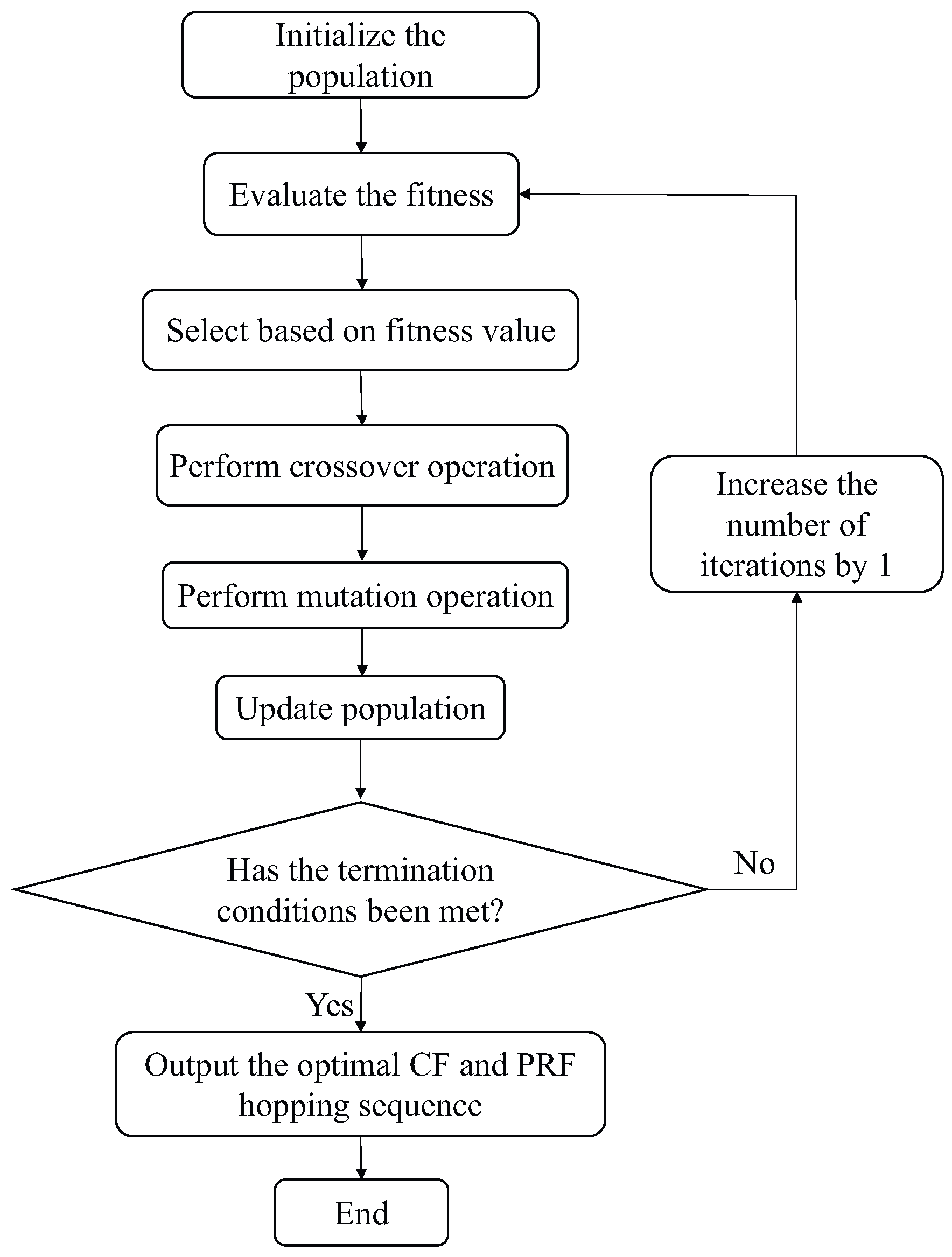
4.2. Joint Optimization of CF-PRF Hopping Sequence for FAR Based on GA

A GA is an optimization algorithm inspired by the principles of biological evolution [26]. The core of this algorithm is to simulate the process of biological evolution and use operations such as selection, crossover and mutation to search for the optimal solution. Its workflow can be summarized as the following steps. Firstly, the population is randomly initialized, and the fitness of each individual is evaluated to determine its selection probability. Next, the selection operation is applied to determine high-quality individuals based on individual fitness. Following this, the crossover operation exchanges the partial chromosomes between two individuals to generate a new individual. Subsequently, mutation operation is utilized to randomly change certain genes of certain individuals, which generates new genetic information. Finally, repeat the above operations continuously until the termination condition is met.
The expression for each element of the dictionary matrix is shown in Equation (18). For the l-th column vector, the corresponding range and velocity are denoted as R i and ν k , respectively, and l = i + P k = 0 , 1 , , P Q 1 . The l-th column vector of the dictionary matrix Ψ can be denoted as ψ l :
ψ l = exp j 4 π m ( n ) Δ f R i c exp j 4 π f 0 ν k t n c 1 + m n Δ f f 0 , n = 0 , 1 , , N 1
Substituting Equation (22) into Equation (21), for the dictionary matrix, its MCC can be expressed as shown below:
μ ( Ψ ) = max 0 l 1 l 2 P Q 1 ψ l 1 , ψ l 2 ψ l 1 2 ψ l 2 2 = max 0 l 1 l 2 P Q 1 ( 1 N n = 0 N 1 ( e j 4 π m ( n ) Δ f R i 1 c e j 4 π f 0 ν k 1 t n c 1 + m ( n ) Δ f f 0 e j 4 π m ( n ) Δ f R i 2 c e j 4 π f 0 ν k 2 t n c 1 + m ( n ) Δ f f 0 ) | )
where l 1 = i 1 + P k 1 and l 2 = i 2 + P k 2 . At this point, the cost function for the dictionary matrix optimization problem can be formulated as shown below:
f o p t ( μ ( Ψ ) ) = min m ( n ) T r ( n ) μ ( Ψ ) = min m ( n ) T r ( n ) ( max 0 l 1 l 2 P Q 1 ( 1 N n = 0 N 1 ( e j 4 π m ( n ) Δ f R i 1 c e j 4 π f 0 ν k 1 t n c 1 + m ( n ) Δ f f 0 e j 4 π m ( n ) Δ f R i 2 c e j 4 π f 0 ν k 2 t n c 1 + m ( n ) Δ f f 0 ) | ) )
where t n = i = 0 n 1 T r ( i ) . The GA flow for solving the optimization problem presented in Equation (24) is outlined as follows.
  • Step 1:
Generate an initial population of size M ˜ through binary encoding, where each individual’s chromosome is a sequence consisting of a set of CF hopping coefficients and PRFs. Each of the bits in the string represents the gene of each chromosome. Set the initial iteration number i t = 0 and the maximum iteration number i t max = 500 .
  • Step 2:
According to (24), we calculate the fitness of each individual to evaluate their quality. And we use f ˜ ( i ˜ ) to represent the fitness of the i ˜ -th individual, where i ˜ = 1 , 2 , , M ˜ . Individuals with high fitness are more likely to be selected and retained.
  • Step 3:
Perform selection operation. This step employs a reproduction operator based on roulette wheel selection according to the fitness function value evaluated by step 2. During this process, P s ( i ˜ ) = f ˜ ( i ˜ ) j ˜ = 1 M ˜ f ˜ ( j ˜ ) denotes the probability of the i ˜ -th individual being selected, and P l ( i ˜ ) = j ˜ = 1 i ˜ P s ( j ˜ ) represents the cumulative probability of the i ˜ -th individual. Then, random number e ˜ , which is between 0 and 1, is generated and compared with P l ( i ˜ ) to determine the selection individual. If P l ( i ˜ 1 ) < e ˜ < P l ( i ˜ ) , the i ˜ -th individual is selected. Repeated m ˜ rounds are conducted to generate m ˜ individuals of offspring generation, where m ˜ M ˜ .
  • Step 4:
Perform crossover operation on the selected individuals with probability P c . Adopt a single point crossover approach, where only one crossover point is randomly set in an individual’s coding string, and then partial chromosomes of two paired individuals are exchanged at that point to form two new individuals.
  • Step 5:
Perform mutation operation on individuals after crossover operation with probability P m . Replace certain genes in an individual’s chromosome coding string with other alleles to form a new individual.
  • Step 6:
Reinsert the offspring obtained through selection, crossover, and mutation operations into the parent generation to generate a new population, and increase the number of iterations by 1.
  • Step 7:
Determine whether the maximum number of iterations i t max has been reached. If not, loop through steps 2 to 6; otherwise, terminate the loop and output the optimized CF and PRF hopping sequence.
The flowchart for GA processing in the optimization is shown in Figure 3.

5. Simulations

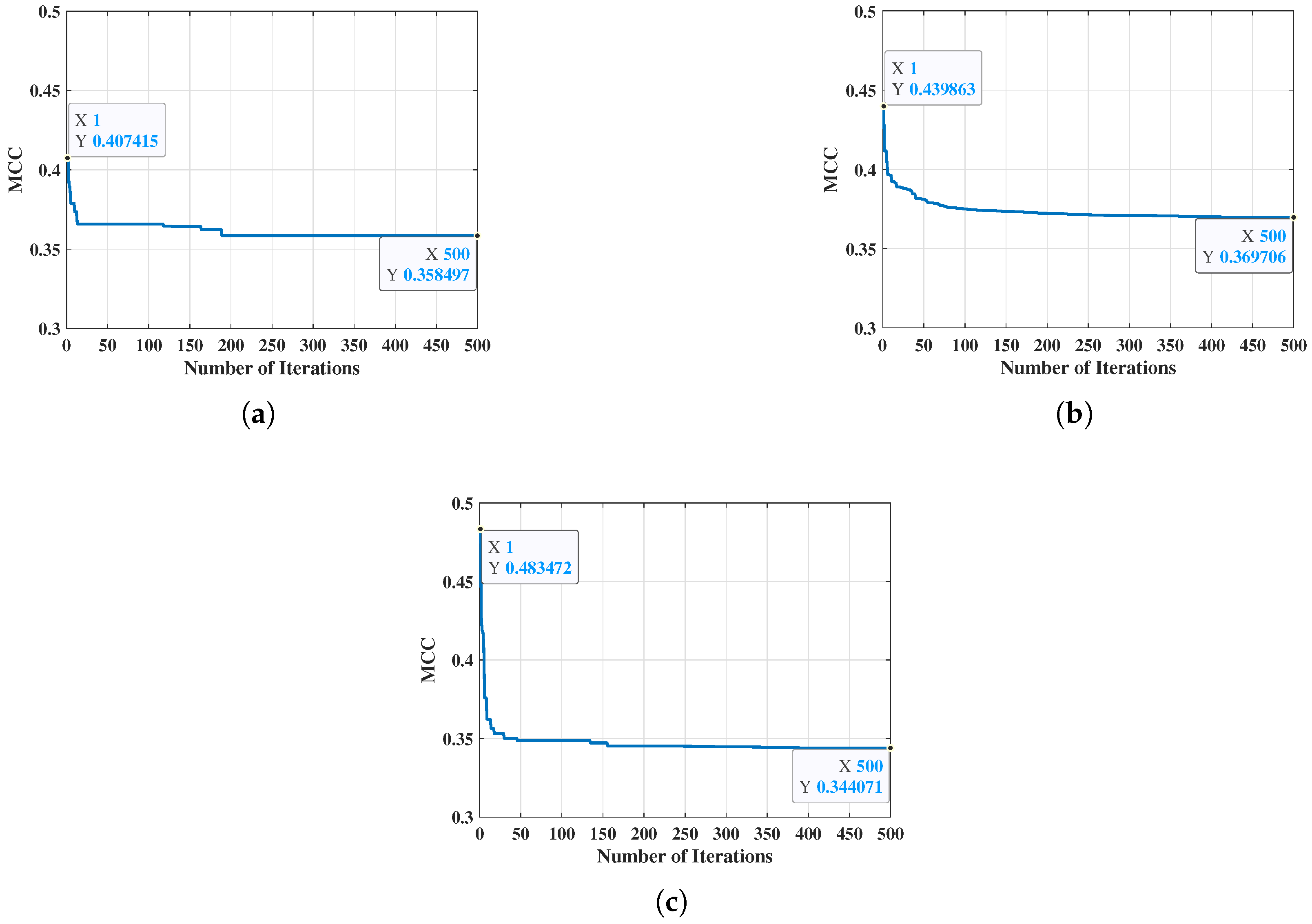
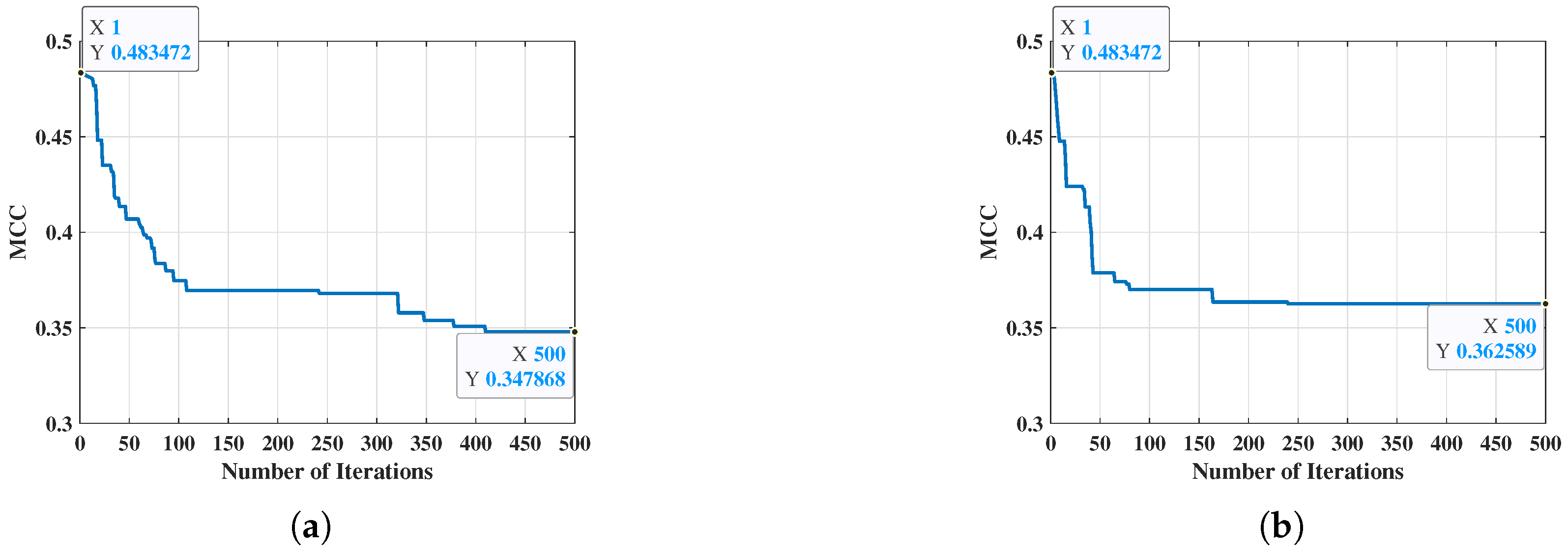
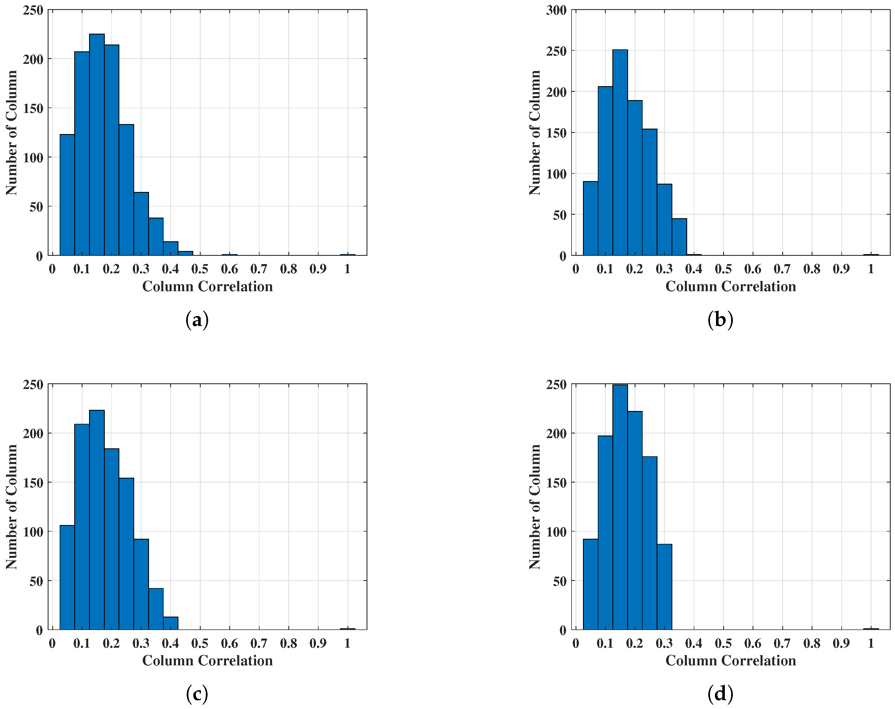
5.1. Optimization Results of Dictionary Matrix

To validate the effectiveness of the aforementioned method, a GA is employed to jointly optimize the CF and PRF hopping coefficients of the CF-PRF jointly agile transmitted signal under the CS framework. To better illustrate the advantages of joint optimization, separate optimization simulations are conducted for the CF hopping coefficients of the CF agile signal and the PRF hopping sequence of the PRF agile signal under identical parameter settings. The radar transmits a CF-PRF jointly agile pulse sequence with an LFM signal. The relevant experimental parameters are summarized in Table 1.
The relevant parameters of the GA are as follows. The population size is 200, which means it has 200 individuals. The iteration number is 500; it has a crossover probability of 0.6 and a mutation probability of 0.01. During the optimization process based on a GA, the MCC of the dictionary matrix for the CF agile signal, PRF agile signals, and CF-PRF jointly agile signal varies with the number of iterations, as shown in the following figures.
As we can see from the Figure 4, when the number of iterations increases, the MCC of the dictionary matrix decreases significantly for all three types of signals. Notably, the CF-PRF jointly agile signal achieves the lowest MCC among the three, which indicates that the joint optimization of CF and PRF can more effectively reduce the correlation between the columns of the dictionary matrix.
In order to compare the performance of the different algorithms, we also optimized Equation (24) using both SA and PSO under the same radar parameters. Like the GA, SA and PSO also iterated from the initial MCC of 0.483472 and iterated 500 times. We performed 50 Monte Carlo trials on each of these three algorithms to compare their average iteration time and average MCC after iterations, which are shown in Table 2. Then, we select one Monte-Carlo trial result each from SA and PSO to display the variation of MCC with the number of iterations as shown in the following figures.
From Table 2 and Figure 5, we can clearly find that the convergence speed of SA is significantly lower than that of PSO and GA. In contrast, PSO has the fastest iteration speed among the three algorithms, but its optimization effect is not as good as the other two algorithms. Furthermore, we can find that after iterating the same number of times, the optimized dictionary’s MCC of the CF-PRF jointly agile signal based on GA is lower than that based on PSO and SA. For the above considerations, we adopted the CF and PRF hopping sequences optimized by the GA for subsequent simulation experiments. The optimized CF hopping coefficients for the CF agile signal, the optimized PRF sequence for the PRF agile signal, and the optimized CF hopping coefficients and PRFs for the CF-PRF jointly agile signal, which are all based on the GA, are presented in Table 3, Table 4 and Table 5, respectively.
Table 2. The performance comparison of GA, SA, and PSO.
GASAPSO
Average Iteration Time58765 s74928 s17081 s
Average MCC0.3450920.3495630.361284
Due to the large dimensionality of the dictionary, only the correlation between the middle column and other columns is statistically represented. The correlation coefficients between the middle column and other columns before and after optimization are illustrated in the Figure 6.
From the Figure 6, it can also be observed that the correlation between columns of the dictionary matrices constructed from the three types of signals is significantly reduced after optimization. To more intuitively illustrate the reduction of correlation, the histograms in Figure 7 are used to represent the correlation between the middle column and other columns of the dictionary matrices generated by the three signals before and after optimization.
From the histograms, it can be observed that the dictionary matrix without optimization exhibits the highest column correlation. The dictionary matrix optimized for CF shows lower correlation compared to that optimized for PRF. The dictionary matrix optimized jointly for CF and PRF achieves the lowest correlation whose values are predominantly below 0.3.

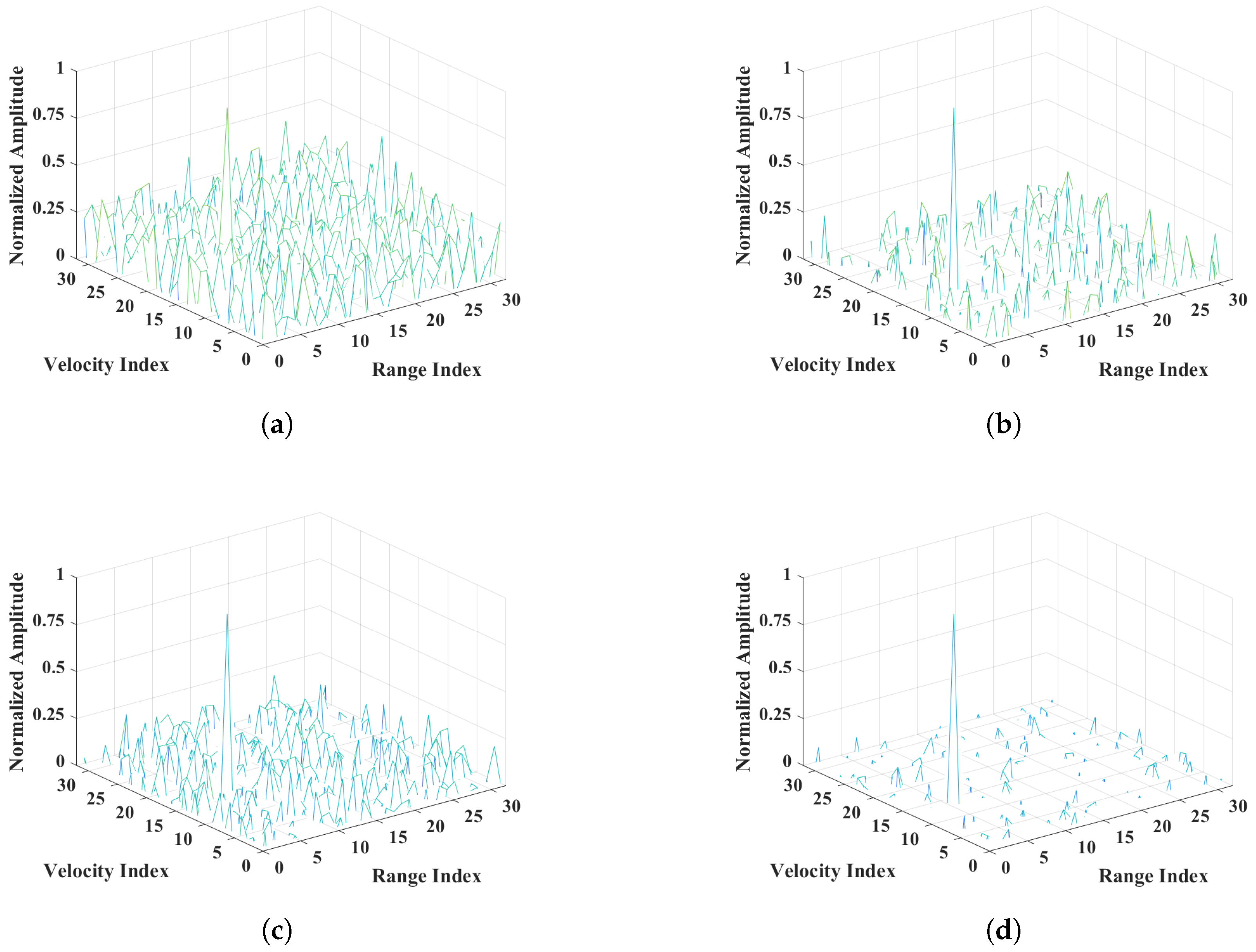
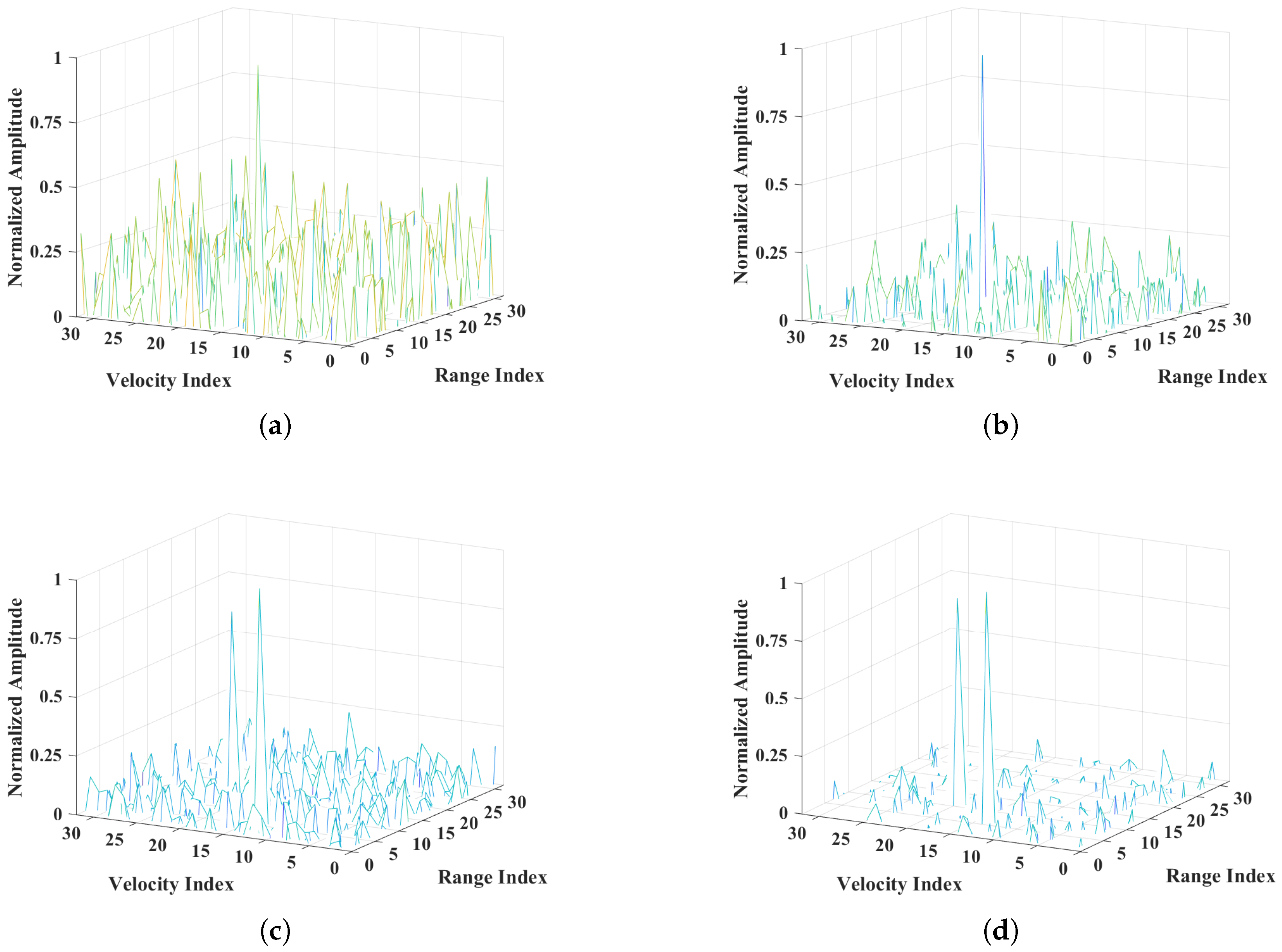
5.2. Reconstruction Results Using ADMM

To more intuitively demonstrate the effects of the optimized CFs and PRFs, sparse reconstruction based on the ADMM is performed using the optimized CFs and PRFs. In the single-target scenario of tracking radar, assume a point target is located at a distance of 10 , 000 m from the radar and moving toward the radar at a radial velocity of 25 m / s . And for multi-target scenarios, the ranges and velocities of the targets are target 1 [ 10 , 012 m , 31 m / s ] and target 2 [ 10 , 023 m , 52 m / s ], respectively. On the basis of the parameters in Table 1 and Table 5, calculate range and velocity resolutions Δ r = c 2 B = c 2 M Δ f 2.3 m , Δ ν = c 2 f 0 T 2.6 m / s , where T = i = 0 N 1 T r ( i ) denotes the total transmission time of N pulses within a CPI. By this means, we can divide the observation scene into 32 high-resolution range and 32 velocity units, and N l o g ( P Q / N ) = 32 l o g ( 1064 / 32 ) > K , where K is the sparsity, i.e., the number of the target expected. Then, we can construct a dictionary matrix. The reconstruction results of the CF agile signal, the PRF agile signal and the CF-PRF jointly agile signal for single-target and multi-target scenarios are shown in Figure 8 and Figure 9, respectively.
Table 3. Optimized CF hopping coefficients for the CF agile signal.
Pulse Number12345678910111213141516
CF hopping coefficient9211114241511141214142628422
Pulse Number17181920212223242526272829303132
CF hopping coefficient253110319813217241401183113
Table 4. Optimized PRFs for the PRF agile signal.
Pulse Number12345678910111213141516
PRI (μs)0605662606601661626657602600644632602612606600
Pulse Number17181920212223242526272829303132
PRI (μs)600600600647647663606600663624610625662663602603
Table 5. Optimized CF hopping coefficients and PRFs for the CF-PRF jointly agile signal.
Pulse Number12345678910111213141516
CF hopping coefficient1222172961581919153110715624
PRI (μs)0605607600601603626613615653656602609608607647
Pulse Number17181920212223242526272829303132
CF hopping coefficient2121016817196481610025289
PRI (μs)651604600603620626615602633654640600630605636625
As clearly shown in Figure 8 and Figure 9, when sparse reconstruction is performed without any parameter optimization, the reconstructed results exhibit relatively high sidelobes, which are attributed to the strong correlation between the columns of the dictionary matrix. Especially for multi-target scenarios, high sidelobes will overwhelm weak targets, which leads to missed detections. After separately optimizing the CF and PRF of the transmitted signal, the correlation between the columns of the dictionary matrices is reduced, which contributes to reconstructed results with lower sidelobe levels. However, these lower sidelobes still have a negative impact on target detection performance and can still increase the probability of false alarm. Furthermore, when the transmitted pulse sequence employs jointly optimized CF-PRF parameters, the reconstructed results achieve even lower sidelobe levels compared to those with individually optimized parameters, which effectively improves the target detection performance and reduces the probability of false alarm.

6. Conclusions

In this paper, a radar signal with joint CF and PRF agility is designed. The signal processing model and dictionary matrix are constructed. Aiming to reduce the correlation of the dictionary matrix, the CF and PRF hopping sequences are optimized through a GA. Finally, the optimized FAR signal is reconstructed using the ADMM. Simulation results demonstrate that the dictionary matrix obtained from the joint CF and PRF optimization method exhibits lower sidelobe levels compared to those obtained through separate optimizations of CF or PRF hopping sequences, which means better target detection performance and lower false alarm probability.

Author Contributions

Conceptualization, H.Z. and Y.Z.; methodology, Z.Y. and H.Z.; software, Z.Y.; validation, Z.Y. and J.Y.; investigation, H.Z. and Y.J.; writing—original draft preparation, Z.Y.; writing—review and editing, H.Z. and Z.Y.; supervision, J.Y. All authors have read and agreed to the published version of the manuscript.

Funding

This work was supported by the Natural Science Foundation of lnner Mongolia Autonomous Region of China under Grants 2023QN06003 and 2021JQ07, the National Natural Science Foundation of China under Grants 62461047 and 62361046, the Young Talents of Science and Technology in Universities of Inner Mongolia Autonomous Region under Grant NJYT22109, the Training Plan for Young Innovative of Grassland Talents Project in Inner Mongolia Autonomous Region under Grant Q2022003, and the Innovation Capability Support Program of Shaanxi under Grant 2023KJXX-015.

Data Availability Statement

The original contributions presented in the study are included in the article; further inquiries can be directed to the corresponding author.

Conflicts of Interest

The authors declare no conflicts of interest.

References

  1. Skolnik, M. An introduction and overview of radar. In Radar Handbook; McGraw-Hill: New York, NY, USA, 2008; Volume 3, pp. 1.1–1.24. [Google Scholar]
  2. Suo, P.C.; Tao, S.; Tao, R.; Nan, Z. Detection of high-speed and accelerated target based on the linear frequency modulation radar. IET Radar Sonar Navig. 2014, 8, 37–47. [Google Scholar] [CrossRef]
  3. Axelsson, S.R. Analysis of random step frequency radar and comparison with experiments. IEEE Trans. Geosci. Remote Sens. 2007, 45, 890–904. [Google Scholar] [CrossRef]
  4. Alland, S.; Stark, W.; Ali, M.; Hegde, M. Interference in automotive radar systems: Characteristics, mitigation techniques, and current and future research. IEEE Signal Process. Mag. 2019, 36, 45–59. [Google Scholar] [CrossRef]
  5. Zhang, L.; Qiao, Z.j.; Xing, M.; Li, Y.; Bao, Z. High-resolution ISAR imaging with sparse stepped-frequency waveforms. IEEE Trans. Geosci. Remote Sens. 2011, 49, 4630–4651. [Google Scholar] [CrossRef]
  6. Wehner, D.R. High Resolution Radar; Artech House, Inc.: Norwood, MA, USA, 1987; 484p. [Google Scholar]
  7. Liu, Y.; Meng, H.; Li, G.; Wang, X. Range-velocity estimation of multiple targets in randomised stepped-frequency radar. Electron. Lett. 2008, 44, 1032–1034. [Google Scholar] [CrossRef]
  8. Eldar, Y.C.; Kutyniok, G. Compressed Sensing: Theory and Applications; Cambridge University Press: Cambridge, UK, 2012. [Google Scholar]
  9. Eldar, Y.C. Sampling Theory: Beyond Bandlimited Systems; Cambridge University Press: Cambridge, UK, 2015. [Google Scholar]
  10. Ruixue, Z.; Guifen, X.; Yue, Z.; Hengze, L. Coherent signal processing method for frequency-agile radar. In Proceedings of the 2015 12th IEEE International Conference on Electronic Measurement & Instruments (ICEMI), Qingdao, China, 16–18 July 2015; Volume 1, pp. 431–434. [Google Scholar]
  11. Lu, Y.; Tang, Z.; Zhang, Y.; Yu, L. Maximum unambiguous frequency of random PRI radar. In Proceedings of the 2016 CIE International Conference on Radar (RADAR), Guangzhou, China, 10–13 October 2016; pp. 1–5. [Google Scholar]
  12. Pan, J.; Chen, Z.; Hu, P.; Bao, Q.; Xu, S. Coherent integration method of high-speed target for random PRI and staggered PW radar. In Proceedings of the 2019 PhotonIcs & Electromagnetics Research Symposium-Spring (PIERS-Spring), Rome, Italy, 17–20 June 2019; pp. 1037–1042. [Google Scholar]
  13. Yang, J.; Thompson, J.; Huang, X.; Jin, T.; Zhou, Z. Random-frequency SAR imaging based on compressed sensing. IEEE Trans. Geosci. Remote Sens. 2012, 51, 983–994. [Google Scholar] [CrossRef]
  14. Quan, Y.; Li, Y.; Wu, Y.; Ran, L.; Xing, M.; Liu, M. Moving target detection for frequency agility radar by sparse reconstruction. Rev. Sci. Instrum. 2016, 87, 094703. [Google Scholar] [CrossRef] [PubMed]
  15. Akhtar, J.; Olsen, K.E. Frequency agility radar with overlapping pulses and sparse reconstruction. In Proceedings of the 2018 IEEE Radar Conference (RadarConf18), Oklahoma City, OK, USA, 23–27 April 2018; pp. 0061–0066. [Google Scholar]
  16. Huang, T.; Liu, Y. Compressed sensing for a frequency agile radar with performance guarantees. In Proceedings of the 2015 IEEE China Summit and International Conference on Signal and Information Processing (ChinaSIP), Chengdu, China, 12–15 July 2015; pp. 1057–1061. [Google Scholar]
  17. Tao, Y.; Zhang, G.; Tao, T.; Leng, Y.; Leung, H. Frequency-agile coherent radar target Sidelobe suppression based on sparse Bayesian learning. In Proceedings of the 2019 IEEE MTT-S International Microwave Biomedical Conference (IMBioC), Nanjing, China, 6–8 May 2019; Volume 1, pp. 1–4. [Google Scholar]
  18. Zhen, L.; Wei, X.-z.; Li, X. Novel method of unambiguous moving target detection in pulse-Doppler radar with random pulse repetition interval. J. Radars 2012, 1, 28–35. [Google Scholar]
  19. Liu, Z.; Wei, X.; Li, X. Aliasing-free moving target detection in random pulse repetition interval radar based on compressed sensing. IEEE Sens. J. 2013, 13, 2523–2534. [Google Scholar] [CrossRef]
  20. Sui, J.; Liu, Z.; Wei, X.; Li, X. Velocity false target identification based on random pulse repetition interval compressed sensing radar. Acta Electron. Sin 2017, 45, 98–103. [Google Scholar]
  21. Du, S.; Quan, H.; Sha, M. Waveform optimization for SFA radar based on evolutionary particle swarm optimization. Syst. Eng. Electron. 2022, 44, 834–840. [Google Scholar]
  22. Donoho, D.L.; Tanner, J. Neighborliness of randomly projected simplices in high dimensions. Proc. Natl. Acad. Sci. USA 2005, 102, 9452–9457. [Google Scholar] [CrossRef] [PubMed]
  23. Deng, W.; Yin, W. On the global and linear convergence of the generalized alternating direction method of multipliers. J. Sci. Comput. 2016, 66, 889–916. [Google Scholar] [CrossRef]
  24. Shapiro, J. Genetic algorithms in machine learning. In Advanced Course on Artificial Intelligence; Springer: Berlin/Heidelberg, Germany, 1999; pp. 146–168. [Google Scholar]
  25. Candes, E.J.; Romberg, J.K.; Tao, T. Stable signal recovery from incomplete and inaccurate measurements. Commun. Pure Appl. Math. 2006, 59, 1207–1223. [Google Scholar] [CrossRef]
  26. Lambora, A.; Gupta, K.; Chopra, K. Genetic algorithm-A literature review. In Proceedings of the 2019 International Conference on Machine Learning, Big Data, Cloud and Parallel Computing (COMITCon), Faridabad, India, 14–16 February 2019; pp. 380–384. [Google Scholar]
Figure 1. CF-PRF variation diagram.
Remotesensing 17 01796 g001
Figure 2. CS processing flowchart.
Remotesensing 17 01796 g002
Figure 3. GA flowchart.
Remotesensing 17 01796 g003
Figure 4. The objective function value vs. iteration number based on GA: (a) CF agile signal; (b) PRF agile signal; (c) CF-PRF jointly agile signal.
Remotesensing 17 01796 g004
Figure 5. The dictionary’s MCC of CF-PRF jointly agile signal vs. iteration number: (a) SA; (b) PSO.
Remotesensing 17 01796 g005
Figure 6. The correlation comparison between the optimized dictionary and unoptimized dictionary: (a) CF agile signal; (b) PRF agile signal; and (c) CF-PRF jointly agile signal.
Remotesensing 17 01796 g006
Figure 7. Histogram of correlation coefficients between the middle column and other columns of the dictionary matrix: (a) before optimization; (b) after CF optimization; (c) after PRF optimization; and (d) after CF-PRF joint optimization.
Remotesensing 17 01796 g007
Figure 8. Sparse reconstruction results for single-target scenario: (a) before optimization; (b) after CF optimization; (c) after PRF optimization; (d) after CF-PRF joint optimization.
Remotesensing 17 01796 g008
Figure 9. Sparse reconstruction results for multi-target scenario: (a) before optimization; (b) after CF optimization; (c) after PRF optimization; (d) after CF-PRF joint optimization.
Remotesensing 17 01796 g009
Table 1. Radar simulation parameters.
PRI ( T r ( n ) )600–663 μ s
Pulse width ( τ )20 μ s
Initial CF ( f 0 )3 GHz
Number of pulses ( N )32
Number of available CF points ( M )32
Pulse bandwidth ( B 0 )2 MHz
Frequency hopping Interval ( Δ f )2 MHz
Signal-to-noise ratio ( SNR )0 dB
Disclaimer/Publisher’s Note: The statements, opinions and data contained in all publications are solely those of the individual author(s) and contributor(s) and not of MDPI and/or the editor(s). MDPI and/or the editor(s) disclaim responsibility for any injury to people or property resulting from any ideas, methods, instructions or products referred to in the content.

