Robust GNSS/INS Tightly Coupled Positioning Using Factor Graph Optimization with P-Spline and Dynamic Prediction

Abstract

The combination of GNSS RTK and INS offers complementary advantages but faces significant challenges in urban canyons. Frequent cycle slips in carrier phase measurements and ambiguity resolution algorithms increase computational burden without improving positioning accuracy. Additionally, environmental interference introduces noise into observations, potentially leading to complete signal loss. To address these issues, this paper proposes a factor graph optimization (FGO) positioning algorithm incorporating predictive observation factors. First, a penalized spline (P-spline) is constructed to predict and smooth Doppler measurements. The predicted Doppler is then fused with the dynamics model predictions to enhance robustness. Using predictive Doppler, carrier phase and pseudorange observations are reconstructed, generating predictive constraint factors to improve positioning accuracy. Real-world tests conducted in urban canyons, including Shanghai, demonstrate that the proposed method maintains stable positioning performance even under short-term signal outages, effectively mitigating cumulative positioning errors caused by data loss. Compared to traditional methods that rely solely on available observations, the proposed algorithm improves northward and dynamic positioning accuracy by 35% and 29%, respectively, providing a highly robust navigation solution for complex urban environments.

1. Introduction

High-precision positioning in complex urban environments is crucial for autonomous driving and UAV navigation. As the foundation of multi-sensor fusion positioning, GNSS and INS complement each other, providing continuous, drift-free positioning and forming the minimal sensor configuration for complex scenarios [1]. Traditional GNSS/INS integration commonly employs the Extended Kalman Filter (EKF) framework, which estimates states by locally linearizing nonlinear systems [2,3,4]. However, its single linearization approximation leads to cumulative errors and high sensitivity to outliers in single-epoch observations, requiring additional fault detection mechanisms [5].

At the integration architecture level, the loosely coupled approach [6] offers the advantage of fault isolation; however, it degrades to pure inertial navigation when the number of available satellites is insufficient, leading to rapid accumulation of state estimation errors [7]. The deeply coupled approach [8,9] enhances dynamic performance by leveraging inertial aiding for baseband signal tracking. However, its implementation requires hardware modifications to the GNSS receiver, making it technically complex and cost-prohibitive [10]. The tightly coupled approach [11,12] fuses raw GNSS observations, maintaining positioning capability even when fewer than four satellites are available. Since it operates solely at the algorithm level, the tightly coupled approach represents an optimal balance between reliability and cost, making it the preferred choice for robust urban navigation.

In recent years, FGO has demonstrated superior estimation accuracy and trajectory smoothness due to its ability to incorporate multi-epoch constraints and iterative optimization characteristics [13]. Shen et al. [11] propose a sliding-window-based FGO method for GNSS/INS integration, where state estimates are continuously refined by maintaining a fixed-size set of recent observations while marginalizing older states. This sliding window strategy enhances computational efficiency and ensures robust state estimation, ultimately improving overall positioning accuracy. Furthermore, Dong et al. [14] have introduced an FGO framework for asynchronous data fusion in INS/DVL/USBL integrated underwater navigation. To address the sensitivity of FGO to observation anomalies in complex underwater environments, a sliding window strategy is employed to limit the number of factor nodes and control computational complexity. Additionally, Mahalanobis distance-based anomaly detection is integrated into the factor graph to identify and mitigate faulty measurements, thereby improving the robustness and real-time performance of underwater vehicle navigation. Gao et al. [15] proposed an improved tightly coupled SINS/BPNS (Bionic Polarization Navigation System) integration scheme based on EKF to address the lack of SINS position correction and reliable BPNS measurement screening. A new measurement model and a two-level measurement selection mechanism based on a polarization camera were introduced to enhance navigation performance and robustness in GNSS-denied environments.

Currently, GNSS/INS loosely coupled FGO frameworks primarily integrate GNSS position factors for state estimation [16]. In TC FGO frameworks, the choice of factor integration depends on the specific GNSS positioning strategy. Common implementations include double-difference carrier phase (DDCP) factors [17], carrier phase factors for precise point positioning (PPP) [18], double-difference pseudorange (DDPR) factors [19], and TDCP factors [20].

However, in dense urban environments, frequent satellite signal outages significantly reduce the number of available observations. Traditional FGO approaches construct factors based solely on currently available observations, which leads to insufficient constraint factors when satellite visibility is persistently low. As a result, positioning errors accumulate over time, propagating through the sliding window and degrading state estimation in subsequent epochs. Moreover, available observations often contain cycle slip errors [21] and degraded measurement quality due to multipath interference [22,23] and Doppler anomalies [24].

In the case of complete GNSS observation loss, the remaining visible satellites are typically concentrated at high elevation angles, leading to increased geometric dilution of precision (GDOP) and greater position uncertainty. To address this, some studies have explored GNSS measurement prediction. Li et al. [25] proposed an ARIMA model for time-series-based GNSS position prediction, utilizing pre-outage data for loosely coupled fusion, but it cannot reconstruct raw Doppler and carrier phase observations, making it unsuitable for tightly coupled architectures. The open-loop carrier phase prediction method [26] leverages INS-aided Doppler prediction to control the receiver’s numerically controlled oscillator (NCO), generating continuous phase observations but requiring dedicated hardware modifications. Additionally, it applies only linear prediction to the dynamic component, lacking higher-order motion modeling and noise suppression. Wang et al. [27] have demonstrated the limitations of linear fitting in capturing complex signal variations.

To address these challenges, this paper proposes an FGO positioning algorithm incorporating Doppler prediction, smoothing, and predictive observation factors. The key contributions are as follows:

• Doppler-aided observation reconstruction: To mitigate GNSS signal degradation and outages, a P-spline joint optimization method is introduced. By leveraging cubic spline basis functions and second-order difference regularization, this method predicts missing values while suppressing noise using 5 Hz Doppler data. The integration of 5 Hz sampling with P-splines enhances the regression of nonlinear Doppler variations.The predicted Doppler is fused with dynamic model estimates for enhanced robustness. Carrier phase and pseudorange observations are reconstructed via Doppler integration, reducing reliance on continuous phase tracking and mitigating inertial drift during GNSS outages.
• Predictive tightly coupled FGO framework: To address cycle slip challenges in urban environments, a factor graph is designed, integrating original/predictive DDPR and TDCP factors, and Earth-rotation-compensated IMU pre-integration. The IMU pre-integration accounts for Earth rotation in the ECEF frame and incorporates constraints from predicted GNSS observations. This method effectively mitigates error accumulation in urban environments.
• Multi-scenario validation: The proposed method is evaluated using real-world datasets from urban challenge environments in Beijing, Wuhan, and Shanghai. Results demonstrate continuous and stable positioning under frequent signal blockages, reducing the long-term impact of pre-outage anomalies and data loss while enhancing adaptability to complex urban conditions.

The remainder of this paper is organized as follows. In the discussion of related work, we review existing data prediction methods and FGO-based positioning algorithms. Section 3 details the prediction of raw observations from original data and the construction of FGO constraint factors, followed by experimental evaluation and comparison with state-of-the-art algorithms. Section 4 investigates GNSS vulnerability in urban environments and highlights that incorporating IMU pre-integration and observation prediction into tightly coupled GNSS/INS integration mitigates signal degradation effects. Section 5 concludes the study.

2. Materials and Methods

We first introduce the detailed design of the sliding window FGO framework, followed by the construction of the pre-integration constraint factors, GNSS TDCP constraints, and DDPR constraints. Finally, we present the designed prediction method for missing raw observations.

2.1. Factor Graph Optimization Framework

In factor graphs [28], measurement nodes are not explicitly represented; instead, they are modeled as factor nodes. For the GNSS/INS tightly coupled optimization problem, the corresponding factor graph structure derived from its Bayesian network is illustrated in Figure 1.

As illustrated in the above figure, factor graphs are a class of graphical models that consist of states and factors. The states represent the unknown variables to be estimated in the problem, while the factors are likelihood functions associated with the state nodes they connect, as shown in Equation (1).

$${\Phi }_1(x_1,x_2)=L(x_1,x_2;z_1)\propto p\left(z_1\right|x_1,x_2)$$

(1)

where x represents the state, z denotes the measurement values, and $p(•)$ is the probability density function. The connections between the state nodes and factor nodes are called edges, indicating that the factor depends on these states. Therefore, the form of the factor graph is shown in Equation (2).

$$\Phi \left(\mathbf{X}\right)={\Phi }_3\left(x_2\right)\times {\Phi }_4(x_2,x_3)\times {\Phi }_1(x_1,x_2){\Phi }_2(x_1,x_3)$$

(2)

Here, $\Phi \left(\mathbf{X}\right)$ is the global optimization objective function, and $\Phi \left(\mathbf{X}\right)=L(\mathbf{X};\mathbf{Z})$ represents the corresponding factor. Consequently, the maximum likelihood estimate of the state can be written as shown in Equation (3).

$${\mathbf{X}}_{ML}^{★}=\underset{\mathbf{X}}{\arg \max }\Phi \left(\mathbf{X}\right)$$

(3)

In practical problem modeling, it is typically assumed that measurement noise follows a Gaussian distribution. Additionally, the dimensionality of the measurements is usually smaller than that of the states to be estimated, and under the given measurement data, each constraint factor represents an underdetermined Gaussian distribution function with respect to the states. This means that a single factor cannot fully capture the actual distribution of the associated states. To accurately estimate the state, more constraint factors are required to solve the problem. Under the assumption that measurement noise follows a Gaussian distribution, maximum likelihood estimation is equivalent to the least squares problem. The general form of the measurement function is given in Equation (4).

$$z_k=h_k\left(\mathbf{X}\right)+n_k$$

(4)

Here, ${\mathbf{X}}_k$ denotes the state vector composed of all states associated with the kth measurement, and $n_k\sim N(0,{\Sigma }_k)$. The corresponding form of the kth factor is shown in Equation (5).

$${\varphi }_k\left({\mathbf{X}}_k\right)=exp(-{\displaystyle \frac{1}{2}}\Vert h_k({\mathbf{X}}_{\mathbf{k}}-z_k){\Vert }_{{\Sigma }_k}^2)=exp(-{\displaystyle \frac{1}{2}}\Vert r_k\left({\mathbf{X}}_k\right){\Vert }_{{\Sigma }_k}^2)$$

(5)

Here, $r_k\left(x_k\right)$ is the residual function corresponding to the kth measurement. The factor shown in Equation (5) is applicable to any type of factor. Consequently, the maximum likelihood estimate of the state is equivalent to minimizing the negative log of the global objective function, as expressed in Equation (6).

$${\mathbf{X}}_{ML}^{★}=\underset{\mathbf{X}}{\arg \max }\prod _k{\Phi }_k=\underset{\mathbf{X}}{\arg \min }(-ln\prod _k{\Phi }_k)=\underset{\mathbf{X}}{\arg \min }{\displaystyle \frac{1}{2}}\sum _k{\Vert r_k{\mathbf{X}}_k\Vert }_{{\Sigma }_k}^2$$

(6)

The objective of the least squares problem is to minimize the sum of the squared Mahalanobis distances of the residuals corresponding to all factors in Equation (6), as detailed in Equation (7).

$$C\left(\mathbf{X}\right)={\displaystyle \frac{1}{2}}\sum _k{\Vert r_k\left(X_k\right)\Vert }_{{\Sigma }_k}^2$$

(7)

By stacking the residuals of all factors within the sliding window, a complete residual vector r is formed, as shown in Equation (8).

$$r\left(\mathbf{X}\right)={\left[r_1^{\prime T},r_2^{\prime T},\dots ,r_n^{\prime T},\right]}^T$$

(8)

Each residual is normalized using its corresponding square root information matrix, as denoted by $e_k^{\prime }={\Lambda }_k{r}_k\left({\mathbf{X}}_k\right)$, where ${\Sigma }_k^{-1}={\Lambda }_k^T{\Lambda }_k$. Then final objective function can be expressed as shown in Equation (9).

$$\mathbf{C}\left(\mathbf{X}\right){\displaystyle \frac{1}{2}}{\Vert r\left(\mathbf{X}\right)\Vert }^2$$

(9)

This paper employs an FGO-based sliding window optimizer to integrate IMU pre-integration and raw GNSS observation constraints. Since FGO is a graphical representation of the maximum likelihood estimation (MLE) problem, both MLE and least squares estimation can be formulated as optimal state estimation problems, where the objective function is intuitively represented by the factor graph illustrated in Figure 2.

DDPR refers to the double-differenced pseudorange constraint, TDCP represents the time-differenced carrier phase constraint, and Prediction TDCP denotes the predicted TDCP constraint during carrier phase cycle slips. $x_k$ is the state to be estimated at epoch k within the sliding window, which is specifically formulated as shown in Equation (10).

$$x_k={\left[{\left(p_{e{b}_k}^e\right)}^T,{\left(q_{b_k}^e\right)}^T,{\left(v_{e{b}_k}^e\right)}^T,{\left(b_{g_k}\right)}^T,{\left(b_{a_k}\right)}^T,\delta \dot{d}t\right]}^T$$

(10)

To maintain consistency with the GNSS positioning reference frame, we define position p, attitude quaternion q, and velocity v in the Earth-Centered Earth-Fixed (ECEF) frame, while also including the gyroscope and accelerometer biases, $b_g$ and $b_a$, which are independent of the reference frame. Additionally, we account for the impact of receiver clock drift $\delta \dot{dt}$ on state estimation. Our objective function is to minimize the sum of the normalized residuals of all factors, and the maximum a posteriori (MAP) estimation is formulated as

$$\begin{array}{cc}\hfill {\chi }^{★}& ={argmin}_{\chi ★}(\sum _{k\in [1,n]}\Vert r\left({\widehat{z}}_{k-1,k}^{Pre},\chi \right){\Vert }_{{\Sigma }_{k-1,k}^{Pre}}^2+\sum _{k\in [1,n]}{\Vert r\left({\widehat{z}}_{k,s}^{DDPR},\chi \right)\Vert }_{{\Sigma }_{k,s}^{DDPR}}^2\hfill \\ & +\sum _{k\in [1,n]}\Vert r\left({\widehat{z}}_{k,s}^{TDCP},\chi \right){\Vert }_{{\Sigma }_{k,s}^{TDCP}}^2+\sum _{k\in [1,n]}{\Vert r\left({\widehat{z}}_{k,ps}^{Pre}{-}^{TDCP},\chi \right)\Vert }_{{\Sigma }_{k,pr}^{Pre}TDCP}^2\hfill \end{array}$$

(11)

where $\Sigma$ represents the covariance matrix for each constraint factor, s denotes the satellite IDs that can be used with raw observations, and ps represents the satellites used to construct the TDCP factor with predicted carrier phase.

2.2. IMU Pre-Integration Factor

The residual of the IMU pre-integration factor in Equation (2) can be specifically expressed as shown in the following formula:

$$r_{Pre}({\widehat{z}}_{k-1,k}^{Pre},X)=\left[\begin{array}{c}{C}_e^{b_{k-1}}(r_{b_k}^e-r_{b_{k-1}}^e-v_{b,k}^e\Delta t+0.5g^e\Delta t^2+\Delta p_{g/cor,k-1,k}^e)-\Delta p_{k-1,k}^{Pre}\\ C_e^{b_{k-1}}(v_{b_k}^e-v_{b_{k-1}}^e+g^e\Delta t+\Delta v_{g/cor,k-1,k}^e)-\Delta v_{k-1,k}^{Pre}\\ 2(q_e^{b_{k-1}}\otimes q_{e_{i(k-1)}}^e\otimes q_{b_k}^e\otimes \Delta q_{k-1,k}^{Pre})\\ b_{g_k}-b_{g_{k-1}}\\ b_{a_k}-b_{a_{k-1}}\end{array}\right]$$

(12)

where $C_e^b$ represents the direction cosine matrix (DCM) describing the orientation of the body frame (b) relative to the Earth-Centered Earth-Fixed frame (e) at epoch $k-1$. $g^e$ denotes the gravitational acceleration projected in the e-frame, and $\Delta t$ is the time interval between consecutive epochs. The construction methods for pre-integrated measurements of position ($\Delta p_{k-1,k}^{Pre}$), velocity ($\Delta v_{k-1,k}^{Pre}$), and attitude ($\Delta q_{k-1,k}^{Pre}$) can be found in [6].

2.3. GNSS Constrained Factor

2.3.1. Double-Difference Pseudorange Factor

To mitigate the impact of frequent cycle slips on positioning in urban environments, we use only DDPR as a direct position constraint. The pseudorange observation equations for the rover and base station are given by

$$\begin{array}{cc}\hfill P_r^s& ={\rho }_r^s+c(d{t}_r-d{t}^s)+I_r^s+T_r^s+{ϵ}_r^s\hfill \end{array}$$

(13a)

$$\begin{array}{cc}\hfill P_b^s& ={\rho }_b^s+c(d{t}_b-d{t}^s)+I_b^s+T_b^s+{ϵ}_b^s\hfill \end{array}$$

(13b)

where $\mathit{s}$ denotes the satellite index, while $\mathit{r}$ and $\mathit{b}$ represent the rover and base station, respectively. $\mathit{P}$ denotes the pseudorange observation, and $\rho$ represents the geometric range between the satellite and receiver. $\mathit{c}$ is the speed of light, and $d{t}_r$, $d{t}_b$, and $d{t}^s$ represent the clock biases of the rover, base station, and satellite, respectively. $\mathit{I}$ and $\mathit{T}$ denote the ionospheric and tropospheric errors, while $ϵ$ accounts for unmodeled errors. The single-difference pseudorange between the rover and base station for satellite $\mathit{s}$ is given by

$$\Delta P_{rb}^s=\Delta P_r^s-\Delta P_b^s=\Delta {\rho }_{rb}^s+c\Delta d{t}_{rb}+\Delta I_{rb}^s+\Delta T_{rb}^s+\Delta {ϵ}_{rb}^s$$

(14)

where $\Delta$ denotes the between-station differencing operator, $\Delta {\rho }_{rb}^s$ represents the double-difference geometric range, and $\Delta {dt}_{rb}^s$ denotes the receiver clock bias difference between the rover and base station. Under short-baseline conditions, the ionospheric and tropospheric errors ($\Delta I_{rb}^s$ and $\Delta T_{rb}^s$) are typically assumed to be negligible. Considering a reference satellite t, the between-station single-difference pseudorange equation is expressed as

$$\Delta P_{rb}^t=\Delta P_r^t-\Delta P_b^t=\Delta {\rho }_{rb}^t+c\Delta d{t}_{rb}+\Delta {ϵ}_{rb}^t$$

(15)

From Equations (14) and (15), the double-difference pseudorange (DDPR) expression can be derived as

$$\nabla \Delta P_{rb}^{st}=\Delta P_{rb}^s-\Delta P_{rb}^t=\nabla \Delta {\rho }_{rb}^{st}+\nabla \Delta {ϵ}_{rb}^{st}$$

(16)

where $\nabla \Delta$ represents the double-difference operator. For the DDPR observation factor, we use the following C/N0-based function for covariance modeling:

$${\sigma }_{C/N0}^2=C_0^2\times {10}^{{\displaystyle \frac{max(MAX-C/N0,0)}{10}}}$$

(17)

where ${\sigma }_{C/N0}^2$ is the observation variance; max is the maximum function; and MAX is the predefined maximum C/N0.

2.3.2. TDCP Factor

The observation expression of the GNSS carrier phase of satellite s at epoch k is given by Equation (18).

$$\lambda {\Phi }_k^s=r_k^s+c(\delta t_r-\delta t^s)-I_k^s+T_k^s+\lambda N_k^s+{ϵ}_k^s$$

(18)

where $\lambda$ is the carrier phase wavelength, $\varphi$ represents the carrier phase observation, and $d{t}_r$ and $d{t}^s$ denote the receiver and satellite clock biases, respectively. I and T represent the ionospheric and tropospheric delay errors, respectively. N refers to the carrier phase ambiguity, and $ϵ$ represents other unmodeled errors.

In urban environments, the number of available GNSS carrier phase observations decreases sharply, while frequent cycle slips are introduced. Consequently, relying solely on carrier phases for positioning offers limited benefits and incurs additional computational overhead for ambiguity resolution. Recent studies have increasingly employed TDCP to provide relative position constraints in such environments. In the GNSS/INS tightly coupled framework, even a small number of TDCP constraints can effectively enhance relative positioning accuracy. According to [29], the velocity accuracy estimated using TDCP is an order of magnitude higher than that of Doppler, while also eliminating the need for frequent ambiguity resolution. Therefore, this paper utilizes TDCP to enhance velocity estimation in the FGO state, thereby indirectly improving position accuracy. The TDCP expression is given as follows:

$$\begin{array}{cc}\hfill \Delta {\Phi }_{k-1,k}^s& ={\Phi }_{r_k}^s-{\Phi }_{r_{k-1}}^s\hfill \\ \hfill & =u_k^s(p_{r_{i-1}}^e-p_{s_k}^e)-u_{k-1}^s(p_{r_{i-1}}^e-p_{s_{i-1}}^e)+u_k^s\Delta p_k^{k-1}+c\delta \dot{d}{t}_k^{k-1}+{\epsilon }_{\Delta \Phi }\hfill \end{array}$$

(19)

where $\Phi$ represents the carrier phase observation, $\mu$ denotes the unit line-of-sight (LOS) vector between the satellite and receiver, and $\Delta p_k^{k-1}$ represents the position increment between consecutive epochs. To enhance velocity estimation accuracy, this position increment is computed using the average velocity over adjacent epochs. $\delta \dot{d}{t}_k^{k-1}$ accounts for clock drift errors.

2.4. Observation Data Prediction and Smoothing

In dense urban environments, GNSS signals frequently experience loss of lock. In such cases, the reduction in available satellites significantly increases the PDOP, while the remaining observable satellite data contain substantial errors, leading to a notable increase in positioning errors. This paper employs two strategies to predict and/or smooth Doppler observations:

• Doppler prediction based on satellite ephemeris and INS pre-integration, with compensation for satellite clock drift errors estimated by the FGO algorithm.
• Using P-splines combined with 5Hz observation data for Doppler prediction and smoothing enhances the fitting capability for nonlinear Doppler variations while reducing the impact of observation noise on prediction accuracy.

For dynamics-based Doppler prediction, we assume that the satellite clock drift remains nearly constant between consecutive epochs. Thus, the predicted Doppler value derived from ephemeris, pre-integrated velocity, and clock drift is expressed as

$$f_p=f_{dyna}+f_{\delta dt}=\lambda \times e^T·(v^s-v_r)+f_{\delta dt}$$

(20)

where $f_{dyna}$ represents the projection of the relative dynamics onto the LOS vector, computed from the satellite velocity $v^s$ and the pre-integrated receiver velocity $v_r$. To enhance prediction accuracy, IMU pre-integration considering Earth’s rotation is employed. $\lambda$ denotes the carrier wavelength corresponding to the operating frequency, while $f_{\delta dt}$ accounts for the frequency variation due to clock drift.

The GNSS raw observation data used in this study are sampled at 5 Hz, and a B-spline window covering 6 s (30 data points) is designed to fully capture historical trends during prediction. A cubic B-spline (degree 3) is used for fitting, with an appropriate number of knots selected to balance smoothness and flexibility. Under these parameters, the P-spline smoothing is implemented using the following equation:

$$(B^{T}B+\lambda D^{T}D)\alpha =B^{T}y$$

(21)

where B represents the matrix composed of the values of basis functions evaluated at different knot positions in sequence.

$$B=\left[\begin{array}{cccc}{b}_1\left(x_1\right)& b_2\left(x_1\right)& \dots & b_n\left(x_1\right)\\ b_1\left(x_2\right)& b_2\left(x_2\right)& \dots & b_n\left(x_2\right)\\ ⋮& ⋮& ⋮& ⋮\\ b_1\left(x_m\right)& b_2\left(x_m\right)& \dots & b_n\left(x_m\right)\end{array}\right]$$

(22)

where $i=1,2,\dots ,m$, where m represents the number of knots, and D is the second-order difference matrix, specifically expressed as

$$D_2=\left[\begin{array}{cccccc}1& -2& 1& 0& ...& 0\\ 0& 1& -2& 1& ...& 0\\ ⋮& ⋮& ⋮& ⋮& \ddots & ⋮\\ 0& 0& ...& 1& -2& 1\end{array}\right]$$

(23)

Theory suggests that the smaller the difference between the combination coefficients ${\alpha }_k$ and ${\alpha }_{k+1}$ of adjacent basis functions, the smoother the resulting P-spline curve. We use $\lambda D^{T}D$ as the penalty term, where $\lambda$ is an empirical smoothing factor, to predict and smooth Doppler data while preserving its original trend. This approach reduces the impact of Doppler errors introduced just before signal loss in urban environments, thereby improving velocity estimation. Taking the GPS G06 satellite as an example, we demonstrate the effectiveness of P-spline in predicting and smoothing missing Doppler data in Figure 3. We conducted a centralized P-spline prediction and smoothing experiment on intermittently missing Doppler data of satellite G06 over 300 s, which took only 40 ms to complete.

The blue curve represents the original Doppler data, where frequent data gaps and fluctuations due to obstructions are evident. The P-spline effectively completes missing data and smooths fluctuations. Finally, we fuse the data obtained from both methods, and its impact on system state estimation will be demonstrated in the experimental section. After obtaining the smoothed Doppler predictions, they are used to predict pseudorange and carrier phase data, expressed by the following equations:

$$\begin{array}{cc}\hfill {\phi }_{k+1}& ={\phi }_k+{\int }_{t_k}^{t_{k+1}}{f}_{pre}dt\hfill \end{array}$$

(24)

$$\begin{array}{cc}\hfill {\rho }_{k+1}& ={\rho }_k+\dot{\rho }\times \Delta t={\rho }_k+(-{\displaystyle \frac{f_{pre}\times c}{f_l}})\times \Delta t\hfill \end{array}$$

(25)

By separately applying P-spline prediction and smoothing and dynamics-based Doppler prediction, we constructed robust predicted values for the original observations. The predicted data can be directly used in FGO to construct DDPR and TDCP constraint factors, preventing the degradation of positioning accuracy caused by increased GDOP. Considering that the uncertainty of predicted data accumulates over time, the C/N0 value for prediction is set based on the pre-outage C/N0 with an applied decay factor, formulated as

$$C/N{0}_k=C/N{0}_0\ast {0.96}^k$$

(26)

It is important to note that for satellites with continuous data loss exceeding 15 epochs, observation prediction will be terminated to prevent prediction errors from degrading the final positioning performance.

3. Results

3.1. Experimental Setup

This experiment utilizes two datasets: the public dataset from [30] and the Zhongguancun 0302 dataset. The employed IMUs are HG4930 and ADIS 16465 MEMS IMU. The public dataset includes reference ground truth, while the 0302 dataset uses NovAtel’s SPAN CPT 6 to provide reference ground truth for the ADIS 16465. The key parameters of the three IMUs are listed in the

Table 1. Technical parameters of the IMUs used in the tests. The asterisk “*” denotes the key performance parameters of the IMU. Smaller values indicate better IMU performance.

IMU	HG4930	SPAN-CPT 6	ADIS16465
In-run bias stability of gyroscope (deg/h)	0.35	1	2
$AR{W}^{ *}(\mathrm{deg}/\sqrt{\mathrm{h}})$	0.05	0.0667	0.15
In-run bias stability of accelerometer (mg)	0.05	0.75	$3.6\times {10}^{-3}$
$VR{W}^{ *}(\mathrm{m}/\mathrm{s}/\sqrt{\mathrm{h}})$	0.04	0.1	0.012

below.

The robotic platform used for Zhongguancun experimental data collection is shown in Figure 4.

The comparative methods designed for the experimental section in this study include the following.

RTKLIB (v2.4.2) is a widely used GNSS positioning software package in the GNSS community, supporting DGNSS and Doppler-based velocity estimation. POSGO is a GNSS FGO positioning algorithm designed for urban environments with limited carrier phase availability, incorporating DDPR and TDCP. OB_GINS is a state-of-the-art open-source loosely coupled GNSS/INS positioning framework, which includes preliminary anomaly detection and exclusion mechanisms for GNSS outliers. TC-FGO, proposed in this study, is a tightly coupled FGO algorithm designed for urban environments where the number of observable GNSS satellites is reduced. It utilizes predictive data to construct constraint factors, aiming to mitigate positioning errors caused by observation anomalies and outages while reducing their impact on subsequent epochs within the factor graph window. The state optimization algorithm used by each method, the usage of IMU, the integration strategy, and the type of data employed for velocity estimation are summarized in

Table 2. Sensors and algorithmic techniques used in experimental comparison methods.

Algorithm	Method	IMU	LC/TC	Veocity
RTKLIB	LSQ	off	-	Doppler
POSGO [31]	FGO	off	-	TDCP
OB_GINS [6]	FGO	on	LC	IMU
TC-FGO	FGO	on	TC	TDCP

.

3.2. Experimental Results

3.2.1. Relative Open Scene

To validate the baseline performance of the proposed algorithm, we first conducted experiments using an open-source dataset collected in a relatively open-sky environment in Wuhan. The dataset was acquired in the Fozuling area of Wuhan, where the number of visible GPS + BDS satellites generally remained around 20, dropping to approximately 10 during short-term signal blockages. The minimum PDOP value reached 1.3, indicating favorable satellite geometry and an open observation environment. A comparison of positioning accuracy between the proposed TC-FGO method and RTKLIB is presented in

Table 3. Comparison of positioning results between RTKLIB and TC-FGO in open-sky scenario.

Method	Position $1\mathit{\sigma }$ Error/m			Position $2\mathit{\sigma }$ Error/m
	North	East	Down	North	East	Down
RTKLIB	0.81	0.53	0.95	1.02	1.11	1.52
POSGO	0.56	0.66	0.92	0.75	0.73	1.42
TC-FGO	0.31	0.29	0.66	0.61	0.51	1.36

.

The experimental results demonstrate that POSGO achieves higher positioning accuracy than RTKLIB by jointly optimizing multi-epoch data and employing an iterative refinement strategy. Furthermore, TC-FGO outperforms single-GNSS solutions by incorporating IMU constraints within the FGO framework. Due to short-term signal blockages, a slight increase in the $2\sigma$ positioning error is observed. Figure 5 illustrates the time-distributed positioning error of TC-FGO. The variation in error magnitude reflects the varying degrees of satellite visibility degradation within the selected data segment.

3.2.2. Complex Urban Scenario

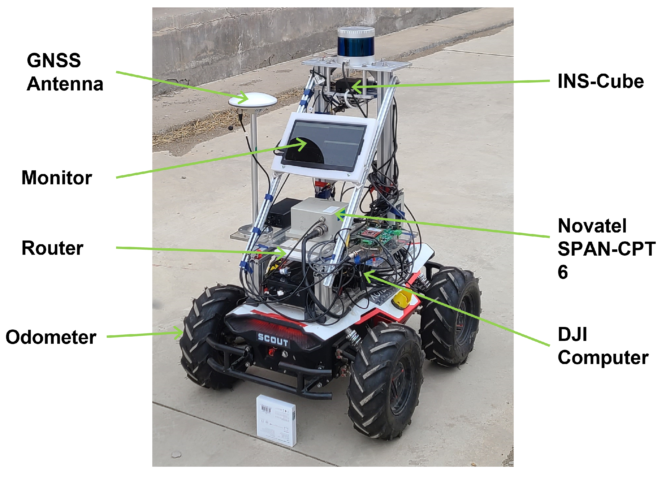
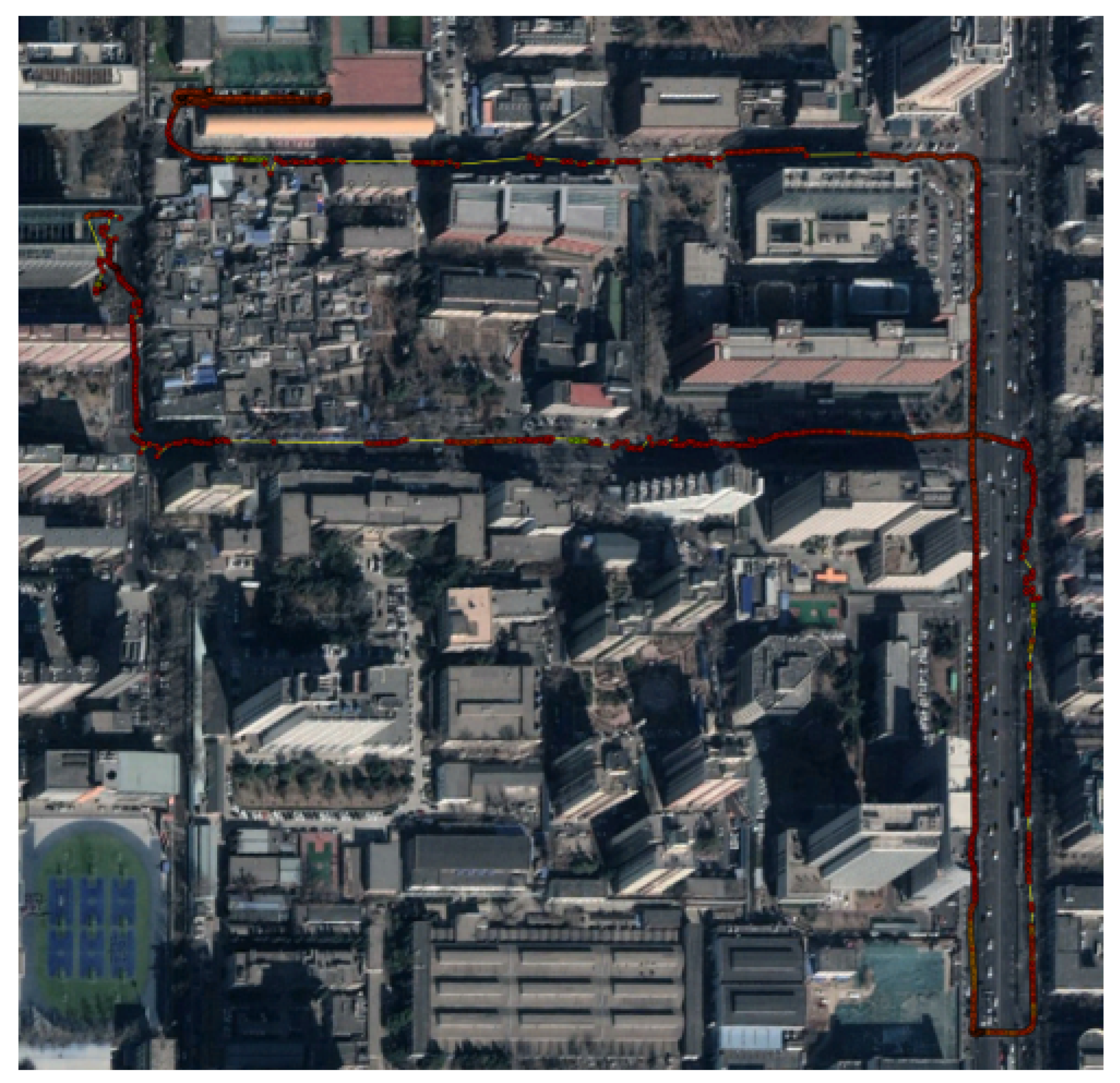
The complex urban environment experiments utilized two different datasets: the Shanghai dataset from the open-source dataset and the robot dataset collected by our team in Zhongguancun, Beijing. The Shanghai dataset consists of 800 s of data from GPS Week 2110 (366,900–367,700) and 1000 s from 372,000–373,000. Notably, the second segment was collected in the Lujiazui area, a dense urban environment where frequent carrier phase loss of lock significantly reduces the availability of carrier phase observations. The Zhongguancun dataset, collected during GPS Week 2140, is illustrated in Figure 6. A 600 s segment (273,850–274,450) was selected, where the robot navigated in close proximity to office buildings and residential complexes, experiencing severe signal blockages. This dataset presents a significant challenge for positioning algorithms due to the intense GNSS signal obstructions.

For the 0302 dataset, as the robot moved close to office buildings and residential complexes, pseudorange multipath errors increased rapidly, and cycle slips occurred in the carrier phase. However, the GNSS receiver failed to effectively detect these errors, resulting in an output position standard deviation smaller than the actual positioning error. Incorrect covariance estimation leads to disturbed GNSS/INS fusion and, through the sliding window mechanism of FGO, propagates its impact to subsequent epochs. As a result, it yields larger positioning error statistics than standalone GNSS, due to the misweighted fusion process amplifying estimation inconsistencies over time. Therefore, a comparison between POSGO and TC-FGO is presented in

Table 4. Position $1\sigma$ and $2\sigma$ errors for the 0302 trajectory segment using different methods.

Method	2D Position Error /m		3D Position Error /m
	1σ	2σ	1σ	2σ
RTKLIB	1.96	5.66	7.69	10.11
POSGO	2.16	3.84	3.71	15.73
OB_GINS	4.74	19.56	11.12	20.69
TC-FGO	1.92	2.88	3.50	7.72

below.

As shown in Table 4 above, complex urban environments introduce significant observational errors into raw GNSS measurements, resulting in rapid degradation of positioning accuracy. For example, RTKLIB exhibits relatively large 3D positioning errors, and the 3D $2\sigma$ error of POSGO exceeds 15 m. In the case of OB_GINS, the receiver continuously provides inaccurate position covariance estimates, which suppresses the contribution of IMU pre-integration during this period. This leads to cumulative positioning errors that propagate through subsequent epochs, ultimately producing larger error statistics than standalone GNSS. In contrast, TC-FGO achieves superior positioning performance by assigning individualized fusion weights to each satellite based on its $C/N_0$ value, and by incorporating finely modeled IMU pre-integration factors.

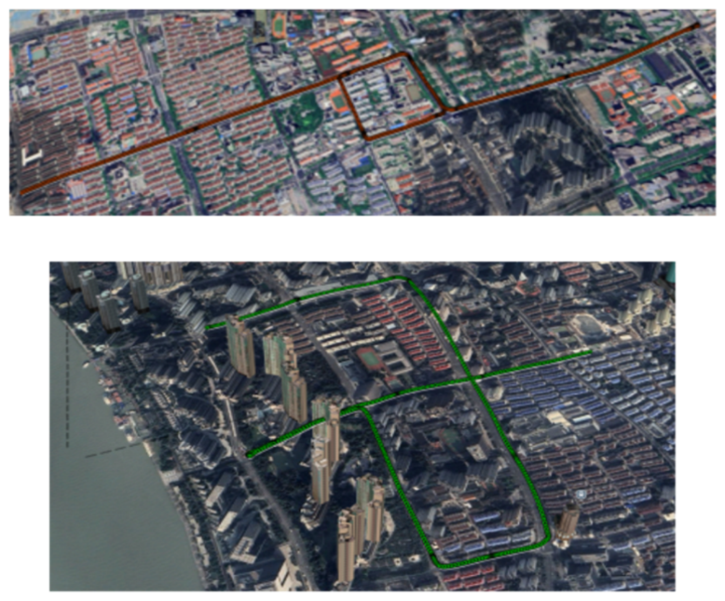
The driving trajectory of the Shanghai Lujiazui dataset is shown in Figure 7 below. In the first data segment, the vehicle traveled through a medium urban environment, where the GNSS receiver experienced brief carrier phase loss-of-lock events. In the second data segment, the vehicle navigated through an area with tall office buildings and dense residential complexes, leading to frequent and extensive satellite signal loss of lock. During this period, only a small portion of carrier phase measurements remained continuously tracked. The frequent cycle slips and re-fixation attempts not only consumed significant computational resources but also failed to yield improvements in positioning accuracy.

For the GNSS/INS loosely coupled positioning algorithm, our tests indicate that the GNSS receiver tends to underestimate positioning uncertainty, leading to anomalous covariance matrices for measurement updates or GNSS position constraint factors. This, in turn, limits the contribution of INS in the positioning estimation process. To address this issue, this study adopts a tightly coupled GNSS/INS fusion scheme, utilizing DDPR to constrain absolute positioning. DDPR effectively mitigates most ionospheric, tropospheric, and receiver clock errors, but it remains susceptible to multipath interference. Therefore, TDCP is introduced to constrain velocity between consecutive epochs. TDCP without cycle slips achieves a velocity estimation accuracy that is an order of magnitude higher than Doppler while also indirectly improving position estimation and aiding INS error compensation. For the first data segment, the positioning results obtained from different algorithms are presented in

Table 5. Position, velocity, and attitude $1\sigma$ errors for the first trajectory segment using different methods.

Method	Position $1\mathit{\sigma }$ Error/m			Velocity $1\mathit{\sigma }$ Error/m/s			Attitude $1\mathit{\sigma }$ Error/°
	North	East	Down	North	East	Down	Roll	Pitch	Yaw
RTKLIB	0.98	1.65	5.98	-	-	-	-	-	-
OB_GINS	1.43	1.80	7.17	0.15	0.18	0.20	0.20	0.23	1.89
TC-FGO	0.73	0.61	1.63	0.12	0.08	0.25	0.13	0.08	1.62

and

Table 6. Position, velocity, and attitude $2\sigma$ errors for the first trajectory segment using different methods.

Method	Position $2\mathit{\sigma }$ Error/m			Velocity $2\mathit{\sigma }$ Error/m/s			Attitude $2\mathit{\sigma }$ Error/°
	North	East	Down	North	East	Down	Roll	Pitch	Yaw
RTKLIB	2.38	2.94	10.91	-	-	-	-	-	-
OB_GINS	15.80	13.72	16.78	0.73	0.53	0.40	0.78	0.62	6.27
TC-FGO	1.67	2.80	3.71	0.29	0.18	0.50	0.29	0.18	2.83

.

From the results presented in Table 4 and Table 5, several conclusions can be drawn. First, single-GNSS positioning is highly susceptible to outliers in individual epochs, leading to significant position jumps. For instance, RTKLIB exhibits maximum positioning errors exceeding 15 m. OB_GINS, a state-of-the-art loosely coupled GNSS/INS positioning algorithm, incorporates IMU pre-integration with Earth rotation compensation to improve relative constraints. However, its loosely coupled measurement weighting strategy limits its performance in complex urban environments. Specifically, loosely coupled positioning algorithms directly use the GNSS receiver’s estimated position uncertainty, which is often smaller than the actual positioning error, limiting INS contributions during poor GNSS signal conditions. As shown in Table 4 and Table 5, due to incorrect GNSS position variance estimates, the $1\sigma$ position error of OB_GINS is even worse than RTKLIB, while the $2\sigma$ error is significantly affected by large positioning outliers, severely impacting the usability of the positioning results. This phenomenon is referred to as an observation model failure [32]. In urban environments, satellite signals are frequently obstructed by buildings, leading to frequent carrier phase loss of lock. As a result, GNSS positioning algorithms degrade to DGNSS- or even SPP-level accuracy. Moreover, intermittent GNSS outages cause carrier phase tracking to fall into a re-convergence cycle, consuming significant computational resources without yielding positioning accuracy improvements. The TC-FGO positioning algorithm adopted in this study achieves an optimal balance between positioning accuracy and computational efficiency on the 0302 dataset.

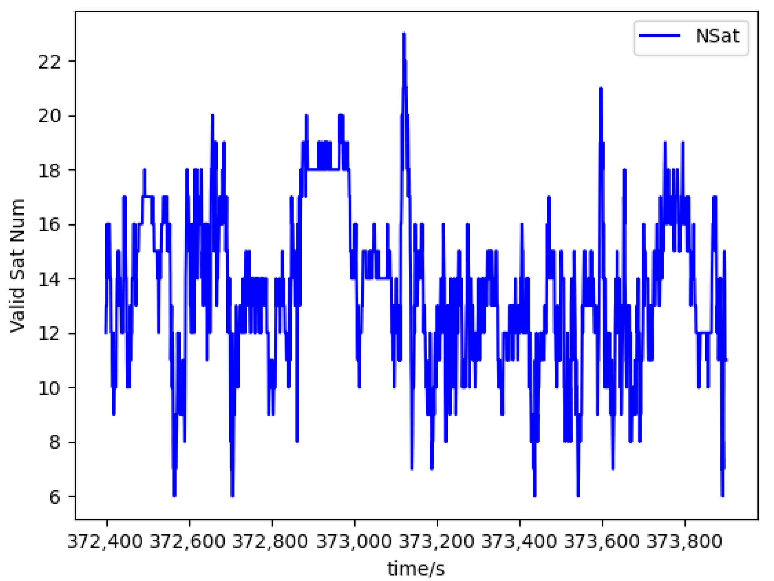
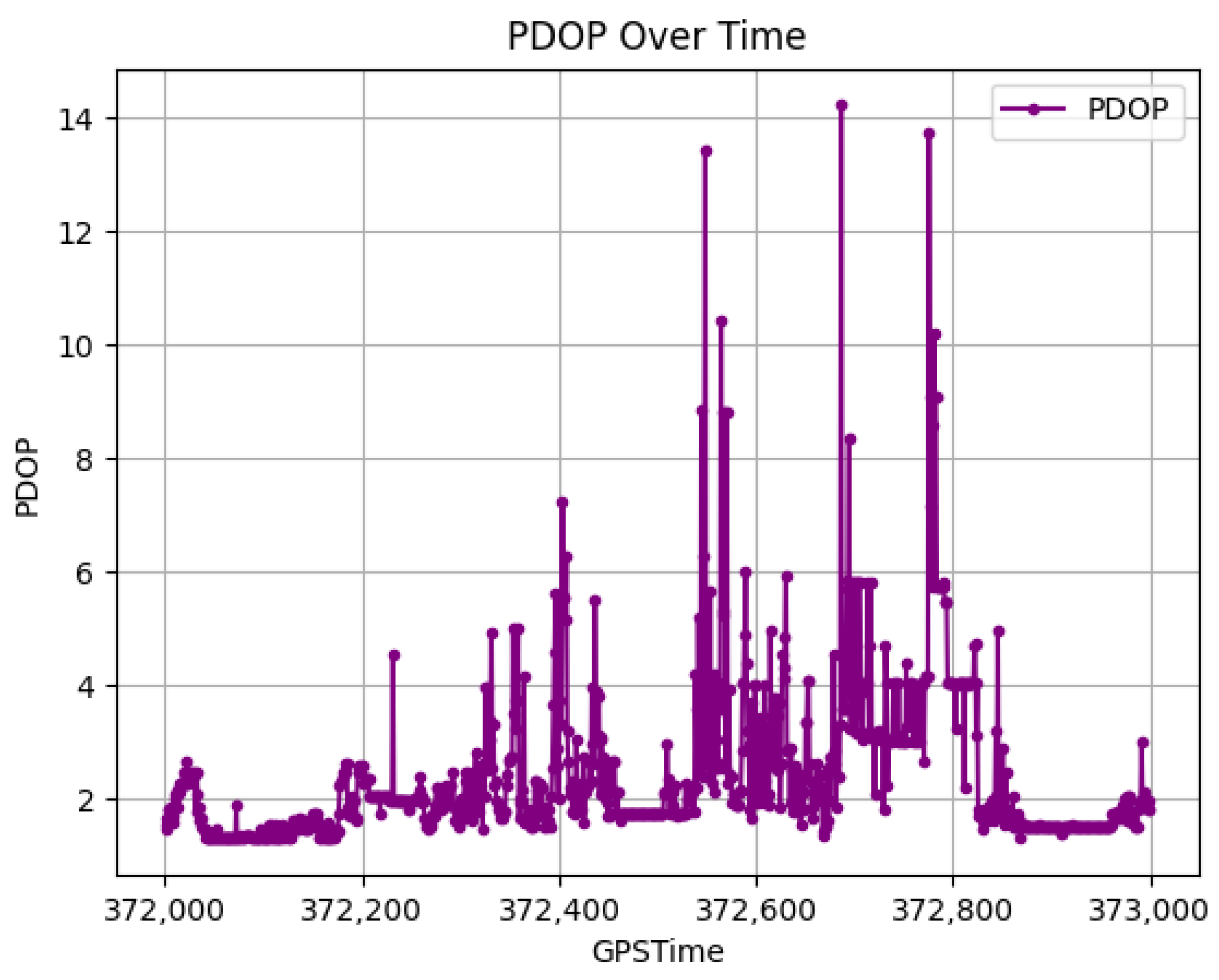
For the second data segment, the variation in the number of tracked satellites is shown in Figure 8. Due to building obstructions along the driving route, the number of trackable GPS and BDS satellites fluctuates significantly, with a substantial number of epochs dropping below 10 satellites. Additionally, the B1I signal of BeiDou-2 exhibits instances of zero observations, and after double-difference (DD) processing, the number of usable satellites is reduced to only 2–3. Moreover, some of the remaining tracked satellites may contain large gross errors. Obstructions result in most participating satellites being at high elevation angles, which leads to a sharp increase in PDOP, as shown in Figure 9. This means to an increase in positioning uncertainty.

In practical positioning algorithms, the number of available satellites frequently falls below four. Data loss not only increases positioning errors in the current epoch but also leads to cumulative errors that persistently affect subsequent epochs. To improve positioning accuracy and continuity, this study employs a series of techniques for observation smoothing and prediction, including Doppler-smoothed pseudorange and P-spline fused dynamic model-based Doppler prediction.

Table 7. Statistical analysis of 3D positioning and velocity $1\sigma$ errors using different methods in a dense urban environment.

Method	Position Error 1$\mathit{\sigma }$/m			Velocity Error 1$\mathit{\sigma }$/m/s
	North	East	Down	North	East	Down
RTKLIB	0.82	3.65	2.22	-	-	-
POSGO	2.72	1.66	6.01	0.03	0.04	0.05
TC-EKF	3.36	2.10	7.62	0.06	0.08	0.14
Origin TC-FGO	1.21	1.25	7.68	0.03	0.05	0.05
Linear Prediction	1.55	1.15	4.13	0.04	0.05	0.06
Ours Prediction	0.96	1.06	2.18	0.02	0.04	0.04

and

Table 8. Statistical analysis of 3D positioning and velocity $2\sigma$ errors using different methods in a dense urban environment.

Method	Position Error 2$\mathit{\sigma }$/m			Velocity Error 2$\mathit{\sigma }$/m/s
	North	East	Down	North	East	Down
RTKLIB	3.82	6.25	5.89	-	-	-
POSGO	4.25	3.35	15.54	0.41	0.51	0.19
TC-EKF	7.84	3.49	18.05	0.26	0.15	0.19
Origin TC-FGO	2.62	2.35	11.78	0.12	0.26	0.21
Linear Prediction	3.50	2.13	9.49	0.13	0.24	0.16
Ours Prediction	1.69	1.68	5.29	0.15	0.24	0.19

below compare the positioning results of RTKLIB and FGO using standalone GNSS data, EKF-based tightly coupled GNSS/INS integration, Doppler-based linear extrapolation, and GNSS/INS tightly coupled integration before and after applying our predictive observation method.

It should be noted that, although RTKLIB supports Doppler-based velocity estimation, the desktop application used in this study does not support velocity output, and thus, the results are not displayed. Both POSGO and TC-FGO utilize TDCP measurements as velocity constraints, while the EKF algorithm estimates velocity based on Doppler measurements. However, as POSGO is a single-GNSS-based solution for positioning and velocity estimation, the number of valid TDCP measurements is significantly reduced in dense urban environments. Consequently, its $2\sigma$ velocity accuracy is noticeably lower than that of tightly coupled methods incorporating IMU pre-integration constraints. In contrast, both EKF and TC-FGO benefit from the assistance of IMU pre-integration, enabling high-precision velocity estimation. The use of more accurate velocity estimates contributes to improved overall positioning accuracy.

In urban environments, the number of available GNSS measurements is limited, and they generally contain varying levels of noise. When the quality of measurement data remains poor over time, FGO accumulates measurement errors from multiple epochs within the optimization window, leading to higher positioning errors in POSGO compared to RTKLIB, which relies on single-epoch positioning. This effect is particularly pronounced in vertical error accumulation [33]. The EKF-based tightly coupled algorithm lacks constraints from historical data, making it highly susceptible to the influence of outliers in single-epoch GNSS measurements. This is primarily because the confidence model based on $C/N_0$ fails to accurately reflect the actual measurement quality under such conditions, leading to a sharp increase in positioning errors. While the original TC-FGO achieves improved horizontal positioning accuracy, it still suffers from significant vertical positioning errors due to persistent poor GNSS observations and cumulative errors in the INS vertical position estimation. Although linear extrapolation of Doppler based on historical data mitigates data loss to some extent, it fails to capture the nonlinear variations caused by vehicle maneuvers, resulting in increased errors in certain directions. By implementing Doppler prediction and smoothing, followed by reconstructing carrier phase and pseudorange observations, the impact of data loss and environmental errors on state estimation is minimized, resulting in the best overall positioning performance.

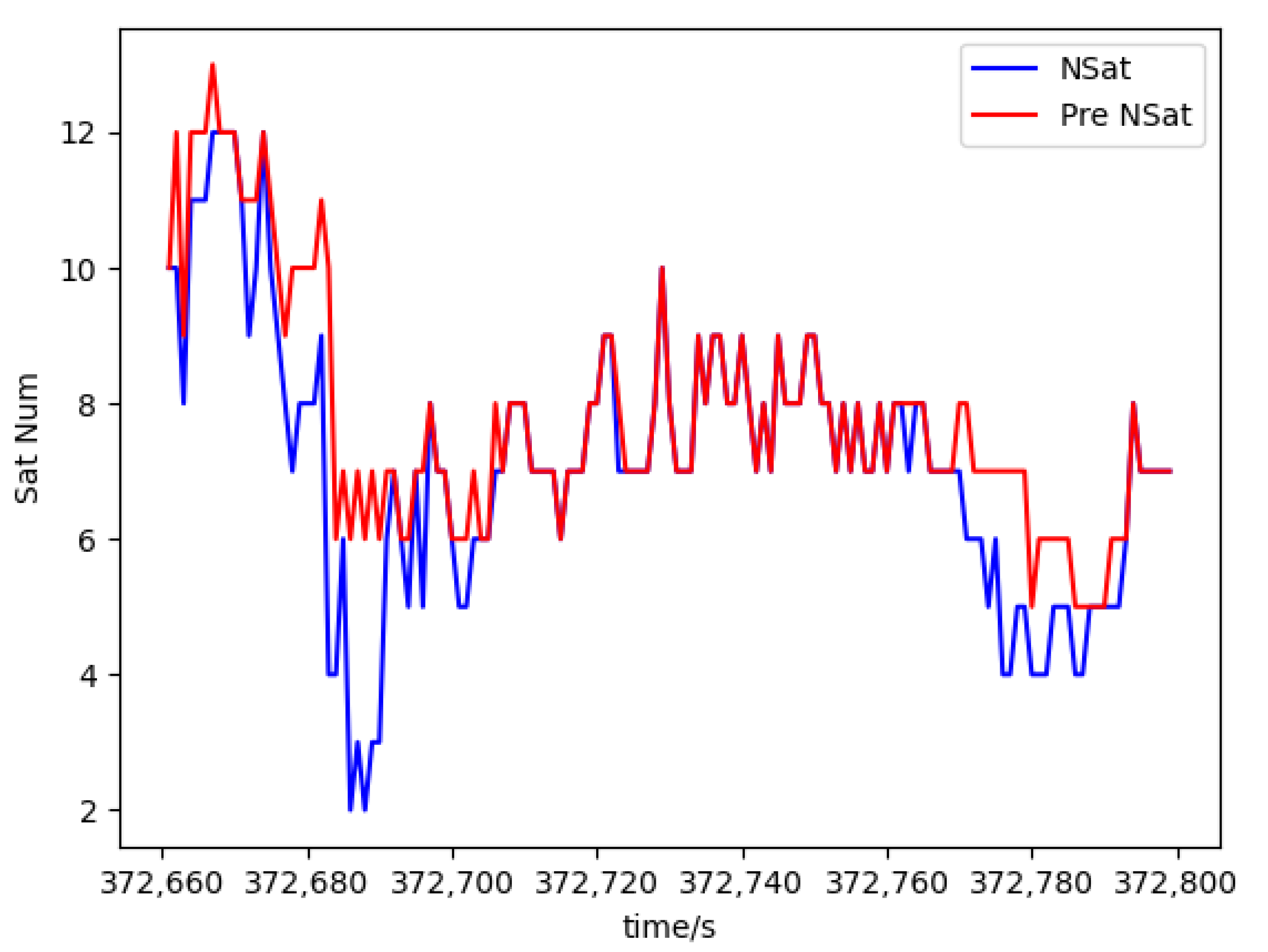
Figure 10 shows a comparison of the number of satellites with available data before and after prediction, where the red line represents the result obtained using our method. As observed, after prediction, the number of available satellites remains above six for most of the time, with a minimum of five in some intervals. In contrast, the original data drop down to two satellites during certain periods. This not only increases positioning errors at those epochs but also affects subsequent epochs through the sliding window mechanism of FGO, until the low-quality data are phased out. Therefore, high-precision prediction and reconstruction of raw observations is essential to improve both positioning accuracy and continuity.

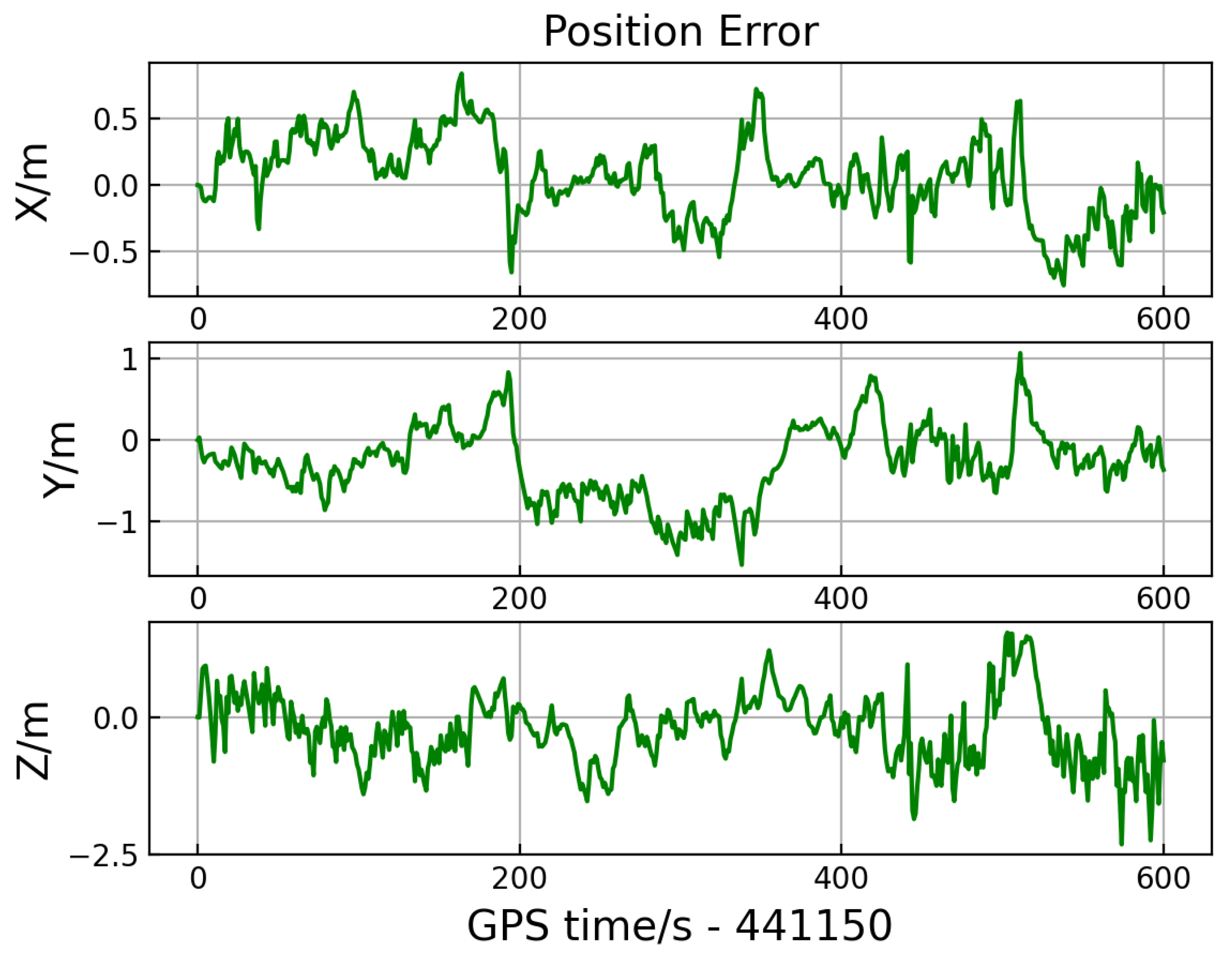
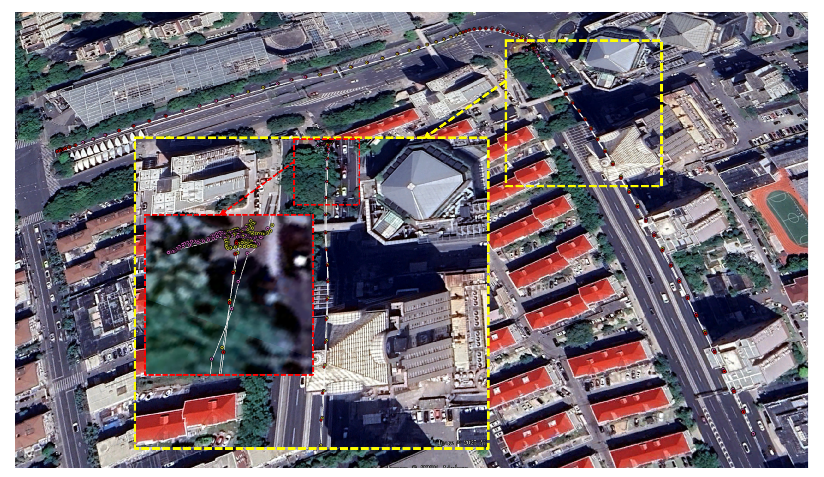
As shown in Figure 11, the trajectory extends from the lower right to the upper left, with a brief stop at the intersection. The red points represent the reference trajectory (ground truth), the pink points indicate the results from the original TC-FGO, and the yellow points represent the TC-FGO enhanced with predictive observations. Due to the presence of surrounding buildings and dense summer foliage, the number of visible satellites gradually decreases, particularly as the vehicle approaches the intersection. As a result, the trajectory derived from the original TC-FGO exhibits noticeable positioning jumps (pink points), and the lack of sufficient satellite observations near the intersection leads to continuous error accumulation. This is evident in the area highlighted by the red dashed box, where the maximum 2D positioning error reaches up to 4.9 m. In contrast, the trajectory using predictive observations (yellow points) demonstrates significantly better positioning consistency, with a maximum error of approximately 2 m. This comparison confirms that incorporating predictive raw observations as constraints effectively contributes to maintaining positioning accuracy under GNSS-degraded conditions.

3.2.3. Execution Time and Efficiency Analysis

This section describes the experimental platform and presents the results of real-time performance evaluation. The experiments were conducted on a system equipped with an Intel Core i5-12650H processor (10 cores, 16 threads, 2.3 GHz base frequency) and 16 GB of DDR4 memory running at 3200 MHz. For raw observation prediction based on satellite and receiver dynamics, we recorded the total execution time and number of epochs, resulting in an average prediction time of 0.28 ms per epoch. For P-spline-based prediction, we measured the average time consumed by the P-spline function to perform prediction and smoothing for each satellite at each epoch, which was approximately 0.029 ms. The core algorithm was implemented in C++, which offers superior execution efficiency and low-level resource control compared to interpreted languages, making it particularly advantageous for applications with strict real-time requirements.

4. Discussion

In urban environments, GNSS observations are highly susceptible to obstructions, often introducing gross errors. However, GNSS receivers fail to accurately assess error levels, and overly optimistic covariance estimates suppress the contribution of INS during degraded GNSS conditions, leading to cumulative positioning errors that can reach the scale of tens of meters. Simply applying fault detection and exclusion algorithms reduces the measurement update frequency, causing INS-only positioning errors to accumulate rapidly. Positioning algorithms that rely solely on raw GNSS observations can independently model observation covariance, but without INS constraints, they remain vulnerable to single-epoch gross errors, resulting in positioning errors exceeding 15 m. Thus, tightly coupled integration is one of the preferred solutions for urban positioning.

In dense urban environments, frequent GNSS signal loss leads to recurrent cycle slips in carrier phase measurements. The high frequency of cycle slips causes positioning algorithms to fall into repeated re-convergence cycles, incurring significant computational costs without improving positioning accuracy. Therefore, in such environments, it is recommended to use DDPR as an absolute position constraint, while TDCP and high-precision IMU pre-integration are employed to constrain the state, enhancing both positioning accuracy and computational efficiency.

When low-elevation satellite signals are blocked, the remaining satellites are predominately concentrated at high elevation angles, causing PDOP to increase rapidly, which leads to a noticable rise in position errors, especially in height. Other sensors can only provide relative position constraints, resulting in continuous error accumulation during GNSS-degraded periods. To mitigate this, high-precision IMU pre-integration combined with satellite dynamics-based Doppler prediction is required to reconstruct carrier phase and pseudorange observations. Additionally, to reduce the impact of IMU pre-integration errors on Doppler prediction, auxiliary methods such as P-spline smoothing are necessary. Cubic basis functions incorporate historical constraints while capturing the current Doppler variation trend, and the second-order difference matrix is used to construct a penalty term, ensuring the prediction process remains robust against noise. By applying these strategies, the impact of data loss on positioning accuracy can be minimized.

The predictive observation algorithm proposed in this study exhibits strong potential for enhancing the continuity and robustness of GNSS positioning systems. By forecasting Doppler measurements and reconstructing pseudorange and carrier phase data, the algorithm can generate predictive observations to sustain continuous positioning in environments with short-term signal outages, such as tunnels and urban areas. Moreover, in complex scenarios, the predicted carrier phase assists in cycle slip recovery and strengthens anomaly detection and correction, effectively mitigating error accumulation and improving positioning reliability. In tightly coupled GNSS/INS systems, when real observations are sparse or unavailable, the predicted observations can be used to update the factor graph estimation, thereby constraining inertial drift and ensuring stable system performance in challenging environments such as urban canyons, tree-lined roads, and tunnels. Overall, by directly compensating for observation-level deficiencies, the proposed method provides strong support for the development of highly robust and continuous navigation systems, with broad potential for practical application.

5. Conclusions

This study proposes a tightly coupled FGO positioning algorithm incorporating Doppler prediction and smoothing to address GNSS signal degradation in urban environments. The method integrates DDPR for absolute positioning constraints while leveraging TDCP and IMU pre-integration to enhance accuracy and efficiency.

The experimental results indicate that frequent GNSS blockages in cities lead to significant degradation in traditional GNSS/INS positioning. Loosely coupled approaches suffer from incorrect GNSS uncertainty estimation, leading to the continuous accumulation of positioning errors. Additionally, frequent cycle slips cause excessive re-convergence cycles, increasing computational costs without accuracy gains. To mitigate these issues, Doppler prediction and smoothing with penalized B-splines reconstruct carrier phase and pseudorange observations during GNSS outages. By combining high-precision IMU pre-integration and satellite dynamics-based Doppler prediction, the method reduces the impact of data loss and environmental errors. P-spline smoothing further enhances robustness by incorporating historical constraints while adapting to rapid variations. Comparative experiments in open-sky, moderate, and dense urban environments show that TC-FGO significantly outperforms RTKLIB, POSGO, and OB_GINS, especially in GNSS-degraded conditions. The method maintains continuous and accurate positioning, mitigating observation anomalies and data loss effects. In conclusion, predictive tightly coupled GNSS/INS integration improves positioning accuracy, robustness, and computational efficiency in urban environments, and shows strong potential for application in scenarios such as short-term GNSS signal interruptions, carrier phase cycle slip repair, and continuous state updating in multi-sensor fusion systems, providing a resilient navigation solution for complex and dynamic environments.

References

1. Eun-Hwan, S.; El-Sheimy, N. Accuracy improvement of low cost INS/GPS for land applications. In Proceedings of the 2002 National Technical Meeting of The Institute of Navigation, San Diego, CA, USA, 28–30 January 2002; pp. 146–157. [Google Scholar]
2. Lu, S.; Gong, Y.; Luo, H.; Zhao, F.; Li, Z.; Jiang, J. Heterogeneous multi-task learning for multiple pseudo-measurement estimation to bridge GPS outages. IEEE Trans. Instrum. Meas. 2020, 70, 1–16. [Google Scholar] [CrossRef]
3. Bao, L.; Luo, H.; Gao, X.; Ning, B.; Zhao, F.; Zhu, Y. MT-e&R: NMEA Protocol-Assisted High-Accuracy Navigation Algorithm Based on GNSS Error Estimation Using Multitask Learning. IEEE Trans. Intell. Transp. Syst. 2022, 23, 20464–20475. [Google Scholar] [CrossRef]
4. Chen, Q.; Lin, H.; Kuang, J.; Luo, Y.; Niu, X. Rapid initial heading alignment for MEMS land vehicular GNSS/INS navigation system. IEEE Sens. J. 2023, 23, 7656–7666. [Google Scholar] [CrossRef]
5. Zhang, Q.; Lin, H.; Ding, L.; Chen, Q.; Zhang, T.; Niu, X. RANSAC-based fault detection and exclusion algorithm for single-difference tightly coupled GNSS/INS integration. IEEE Trans. Intell. Veh. 2023, 9, 3986–3997. [Google Scholar] [CrossRef]
6. Tang, H.; Zhang, T.; Niu, X.; Fan, J.; Liu, J. Impact of the earth rotation compensation on MEMS-IMU preintegration of factor graph optimization. IEEE Sens. J. 2022, 22, 17194–17204. [Google Scholar] [CrossRef]
7. Yu, X.; Guo, Z.; Wu, L. Research on Multi-Source Data Fusion and Satellite Selection Algorithm Optimization in Tightly Coupled GNSS/INS Navigation Systems. Remote Sens. 2024, 16, 2804. [Google Scholar] [CrossRef]
8. Olesen, D.; Jakobsen, J.; Knudsen, P. Ultra-tightly coupled GNSS/INS for small UAVs. In Proceedings of the 30th International Technical Meeting of the Satellite Division of The Institute of Navigation (ION GNSS+ 2017), Portland, OR, USA, 25–29 September 2017; pp. 2587–2602. [Google Scholar] [CrossRef]
9. Zhang, T.; Feng, X.; Niu, X.; Bochkati, M.; Pany, T.; Liu, J. GNSS Carrier Phase Improvement Using a MEMS INS-Aided Long Coherent Architecture for High Precision Navigation. IEEE Trans. Intell. Transp. Syst. 2024, 25, 16745–16760. [Google Scholar] [CrossRef]
10. Chen, S.; Xin, M.; Yang, F.; Zhang, X.; Liu, J.; Ren, G.; Kong, S. Error compensation method of GNSS/INS integrated navigation system based on AT-LSTM during GNSS outages. IEEE Sens. J. 2024, 24, 20188–20199. [Google Scholar] [CrossRef]
11. Shen, Z.; Li, X.; Wang, X.; Wu, Z.; Li, X.; Zhou, Y.; Li, S. A novel factor graph framework for tightly coupled GNSS/INS integration with carrier-phase ambiguity resolution. IEEE Trans. Intell. Transp. Syst. 2024, 25, 13091–13105. [Google Scholar] [CrossRef]
12. Wang, D.; Dong, Y.; Li, Z.; Li, Q.; Wu, J. Constrained MEMS-based GNSS/INS tightly coupled system with robust Kalman filter for accurate land vehicular navigation. IEEE Trans. Instrum. Meas. 2019, 69, 5138–5148. [Google Scholar] [CrossRef]
13. Wen, W.; Pfeifer, T.; Bai, X.; Hsu, L.T. Factor graph optimization for GNSS/INS integration: A comparison with the extended Kalman filter. NAVIGATION J. Inst. Navig. 2021, 68, 315–331. [Google Scholar] [CrossRef]
14. Dong, X.; Hu, G.; Gao, B.; Zhong, Y.; Ruan, W. Windowing-based factor graph optimization with anomaly detection using mahalanobis distance for underwater INS/DVL/USBL integration. IEEE Trans. Instrum. Meas. 2024, 73, 1–13. [Google Scholar] [CrossRef]
15. Gao, B.; Yin, H.; Hu, G.; Zhong, Y. Reliable measurement selection mechanism-based tightly coupled inertial/bionic polarization integration with position correction. Aerosp. Sci. Technol. 2024, 154, 1–14. [Google Scholar] [CrossRef]
16. Li, T.; Zhang, H.; Han, B.; Xia, M.; Shi, C. Relative Accuracy of GNSS/INS Integration Based on Factor Graph Optimization. IEEE Sens. J. 2024, 24, 33182–33194. [Google Scholar] [CrossRef]
17. Li, X.; Yu, H.; Wang, X.; Li, S.; Zhou, Y.; Chang, H. FGO-GIL: Factor graph optimization-based GNSS RTK/INS/LiDAR tightly coupled integration for precise and continuous navigation. IEEE Sens. J. 2023, 23, 14534–14548. [Google Scholar] [CrossRef]
18. Li, T.; Pei, L.; Xiang, Y.; Zuo, X.; Yu, W.; Truong, T.K. P3-LINS: Tightly coupled PPP-GNSS/INS/LiDAR navigation system with effective initialization. IEEE Trans. Instrum. Meas. 2023, 72, 1–13. [Google Scholar] [CrossRef]
19. Wen, W.; Hsu, L.T. Towards robust GNSS positioning and real-time kinematic using factor graph optimization. In Proceedings of the 2021 IEEE International Conference on Robotics and Automation (ICRA), Xi’an, China, 30 May–5 June 2021; pp. 5884–5890. [Google Scholar] [CrossRef]
20. Suzuki, T. Time-relative RTK-GNSS: GNSS loop closure in pose graph optimization. IEEE Robot. Autom. Lett. 2020, 5, 4735–4742. [Google Scholar] [CrossRef]
21. Suzuki, T. GNSS odometry: Precise trajectory estimation based on carrier phase cycle slip estimation. IEEE Robot. Autom. Lett. 2022, 7, 7319–7326. [Google Scholar] [CrossRef]
22. Zhang, T.; Zhou, L.; Feng, X.; Shi, J.; Zhang, Q.; Niu, X. Ins-aided gnss pseudo-range error prediction using machine learning for urban vehicle navigation. IEEE Sens. J. 2024, 24, 9135–9147. [Google Scholar] [CrossRef]
23. Zhang, Q.; Zhang, L.; Sun, A.; Meng, X.; Zhao, D.; Hancock, C. GNSS Carrier-Phase Multipath Modeling and Correction: A Review and Prospect of Data Processing Methods. Remote Sens. 2024, 16, 189. [Google Scholar] [CrossRef]
24. Mouri, A.; Kubo, Y.; Sugimoto, S.; Ohashi, M. Detection and Correction of Doppler Outliers in Kalman Filter-based Positioning. Trans. Inst. Syst. Control Inf. Eng. 2016, 29, 18–28. [Google Scholar] [CrossRef]
25. Li, Q.; Zhang, L.; Wang, X. Loosely coupled GNSS/INS integration based on factor graph and aided by ARIMA model. IEEE Sens. J. 2021, 21, 24379–24387. [Google Scholar] [CrossRef]
26. Li, Z.; Zhang, T.; Qi, F.; Tang, H.; Niu, X. Carrier phase prediction method for GNSS precise positioning in challenging environment. Adv. Space Res. 2019, 63, 2164–2174. [Google Scholar] [CrossRef]
27. Wang, X.; Shi, Y.; Xin, W.; Wang, T.; Yang, G.; Jiang, Z. Channel prediction with time-varying doppler spectrum in high-mobility scenarios: A polynomial fourier transform based approach and field measurements. IEEE Trans. Wirel. Commun. 2023, 22, 7116–7129. [Google Scholar] [CrossRef]
28. Dellaert, F.; Kaess, M. Factor Graphs for Robot Perception. Found. Trends Robot. 2017, 6, 1–139. [Google Scholar] [CrossRef]
29. Suzuki, T. Precise position estimation using smartphone raw GNSS data based on two-step optimization. Sensors 2023, 23, 1205. [Google Scholar] [CrossRef]
30. Zhu, F.; Chen, X.; Cai, Q.; Zhang, X. A large-scale diverse GNSS/SINS dataset: Construction, publication, and application. IEEE Trans. Instrum. Meas. 2024, 73, 1–13. [Google Scholar] [CrossRef]
31. Li, Z.; Guo, J.; Zhao, Q. POSGO: An open-source software for GNSS pseudorange positioning based on graph optimization. GPS Solut. 2023, 27, 1–7. [Google Scholar] [CrossRef]
32. Wang, Q.; Liu, J.; Jiang, J.; Pang, X.; Ge, Z. Application of Improved Fault Detection and Robust Adaptive Algorithm in GNSS/INS Integrated Navigation. Remote Sens. 2025, 17, 804. [Google Scholar] [CrossRef]
33. Li, Z.; Wang, L.; Wang, N.; Li, R.; Liu, A. Real-time GNSS precise point positioning with smartphones for vehicle navigation. Satell. Navig. 2022, 3, 1–22. [Google Scholar] [CrossRef]
Figure 1. Factor graph for GNSS/INS tightly coupled state estimation.
Remotesensing 17 01792 g001
Figure 2. FGO framework based on IMU pre-integration and GNSS raw observation constraints.
Remotesensing 17 01792 g002
Figure 3. Effect of P-spline on predicting and smoothing Doppler data for GPS G06.
Remotesensing 17 01792 g003
Figure 4. The physical platform diagram of the wheeled robot and its carrying reference equipment and test equipment.
Remotesensing 17 01792 g004
Figure 5. Time-distributed NED positioning errors of TC-FGO on the 0115 dataset.
Remotesensing 17 01792 g005
Figure 6. Trajectory map of the robot experiment conducted on 2 March 2022.
Remotesensing 17 01792 g006
Figure 7. The (upper) figure represents a moderate urban environment with relatively low buildings, while the (lower) figure depicts a dense urban environment with taller and more densely distributed buildings.
Remotesensing 17 01792 g007
Figure 8. Number of observable satellites over time.
Remotesensing 17 01792 g008
Figure 9. PDOP variation trend over time.
Remotesensing 17 01792 g009
Figure 10. Comparison of satellite availability before and after prediction.
Remotesensing 17 01792 g010
Figure 11. Trajectory comparison of TC-FGO with and without predictive observations under GNSS-degraded conditions.
Remotesensing 17 01792 g011