Article

The Spatiotemporal Variability of Ozone and Nitrogen Dioxide in the Po Valley Using In Situ Measurements and Model Simulations

1
Laboratory of Atmospheric Physics, Aristotle University of Thessaloniki, 54124 Thessaloniki, Greece
2
TNO, Climate, Air and Sustainability, 3584 CB Utrecht, The Netherlands
*
Author to whom correspondence should be addressed.
Remote Sens. 2025, 17(10), 1794; https://doi.org/10.3390/rs17101794
Submission received: 28 March 2025 / Revised: 9 May 2025 / Accepted: 14 May 2025 / Published: 21 May 2025

Abstract

:
The Po Valley is depicted in the literature as a region with one of the most severe air pollution profiles in Europe, frequently exceeding the permitted statutory concentration limits for several air pollutants. The aim of this paper is to present an assessment of the air quality over the Po Valley for the year 2022 as reported by ground-based air quality monitoring stations of the region and assess chemical transport modeling simulations which can enhance the spatiotemporal reporting in air quality levels which cannot be achieved by the sparse in situ monitoring station coverage. To achieve this, the concentration levels of two significant chemical compounds, namely ozone (O3) and nitrogen dioxide (NO2), are studied here. Measurements include the surface concentrations of in situ measurements from 28 stations reporting to the European Environment Agency (EEA), while chemical transport simulations from the Long-Term Ozone Simulation—European Operational Smog (LOTOS-EUROS) are employed for a comparative analysis of the relative levels observed in each of the two monitoring methods for air quality. The analysis of the EEA stations reports that, for year 2022, all selected monitoring stations exceeded the EU O3 level limit for a minimum of 33 days and the World Health Organization (WHO) limit for a minimum of 78 days. The concentrations of surface O3 and NO2 studied by both the measurements as well as the simulations exhibit a close correlation with the documented diurnal, monthly, and seasonal variability, as previously reported in the literature. The LOTOS-EUROS CTM ozone simulations demonstrate a strong correlation with the EEA measurements, with a monthly correlation coefficient of R > 0.98 and a diurnal correlation coefficient of R > 0.83, indicating that the model is highly effective at capturing the diverse spatiotemporal patterns. The co-variability between ozone and nitrogen dioxide surface levels reported by the EEA in situ measurements reports high R values from −0.76 to −0.88, while the CTM, due to the spatial resolution of the simulations which disables the identification of local effects, reports higher correlations of −0.96 to −0.99. The CTM simulations are hence shown to be able to close the spatial gaps of the in situ measurements and provide a dependable auxiliary tool for air quality monitoring across Europe.

1. Introduction

In the post-industrial revolution times, air pollution has emerged as a dominant environmental concern, pervading numerous regions across the globe. The deterioration of air quality is primarily attributed to population growth, which has resulted in increased energy consumption and industrial production, leading to the release of considerable quantities of deleterious pollutants into the atmosphere. Such pollutants not only impair the air quality but also have an adverse effect on ecosystems, climate, and the overall quality of life [1]. It is therefore imperative to monitor air quality not only to assess immediate health risks but also to gain insight into long-term environmental impacts and develop a more sustainable future.
In this study, the levels of two tropospheric compounds, ozone (O3) and nitrogen dioxide (NO2), are used to investigate the air quality over the Po Valley. Tropospheric O3 is a secondary pollutant that can be transferred from the stratosphere by downward transport to the troposphere [2] and long-range transport [3] but is mainly formed when sunlight interacts with nitrogen oxides (NOx = NO2 + NO), which influence the production and destruction of O3 [4], as well as with volatile organic compounds (VOCs). Similarly, the generation of O3 at the surface (ground-level O3) is also the result of the same photochemical processes as tropospheric ozone. Its variability depends on the combined effects of chemistry, transport, deposition processes [5] and the local meteorological conditions prevailing over a given region [6]. The emissions of NOx in the atmosphere originate from natural processes, primarily as a result of microbial activities in soils and lightning discharges. However, human activities, including the combustion of fossil fuels, biomass burning, and the use of fertilizers, have been identified as the predominant source of NOx emissions [7].
Tropospheric ozone has a short lifetime of a few hours and up to a few weeks elsewhere in locations where its precursors have maximum levels, rendering it a short-lived climate gas [5,8]. The lifetime of NO2 [9,10] is also constrained to a local scale in relation to its source location, and both these facts necessitate the analysis of in situ measurements in addition to the utilization of modeling simulations that facilitate the investigation of the spatial and temporal distribution of the two compounds. Both species demonstrate a discernible diurnal pattern, with O3 showing an early morning onset, a peak in the afternoon, and a subsequent decline in evening ozone levels. At nighttime, ozone surface concentrations are measurable due to the prevalence of mechanisms that outpace ozone destruction, resulting in sustained or even elevated ozone levels. This phenomenon occurs concurrently with the cessation of photochemical production due to the absence of sunlight. The initial mechanism is the chemical reaction whereby, during nocturnal hours, specific compounds, such as peroxyacetyl nitrate (PAN), can undergo a gradual decomposition, resulting in the release of NO2 which, in turn, reacts with O3 precursors [11]. Subsequently, NO2 also reacts with O3 to form nitrate (NO3) radicals, which can react with VOCs or aldehydes, forming organic nitrates that help to stabilize ozone levels [12]. Additionally, the reactions of biogenic volatile organic compounds (BVOCs), such as isoprene or terpenes, with NO3 radicals can result in the generation of secondary organic aerosols (SOAs) and other O3 precursors [13]. Other mechanisms that contribute to the enhancement of surface ozone levels include turbulent mixing, which facilitates the transport of ozone from higher atmospheric layers to the surface [14]; the mixing of O3 from the residual layer; which persists from daytime production to the surface under conditions of stable nocturnal conditions; and the horizontal transport of ozone-rich air from neighboring regions [15], which typically lasts a few hours, and that of NO2 [9], which is constrained to a local scale in relation to its source location, necessitates the analysis of in situ measurements that provide data dependent on the spatiotemporal resolution, in addition to the utilization of modeling simulations that facilitate the investigation of the spatial and temporal distribution of the two compounds. These complex intertwined photochemical and transport processes necessitate the concurrent analysis of both these major air quality-hindering species.
The study area in this work is the Po Valley, a densely inhabited region of Northern Italy, with a population of over 16 million. Ref. [16] frequently documented the Po Valley as one of the most significant hotspots in the literature, exceeding the air quality limit values for numerous pollutants [17,18]. The EU has adopted policies on air quality in order to decrease the exceedances for most air pollutants [19]. In particular, with regard to ozone, Directive 2008/50/EC establishes a long-term target value of 120 μg/m3 and the WHO air quality guideline of 100 μg/m3, which are measured as maximum daily 8 h running average [20].
The Po Valley has been studied in the past due to its known high air pollution levels, particularly ozone and PM10 (e.g., [21]). Ozone concentrations in 1998 often exceeded past international regulations, with peaks reaching up to 200 ppb downwind of Milan [22]. A study examining the budget of pollutants near the surface of the Po Valley [23] concluded that, for half the year, external sources surpassed local contributions. Although local sources predominated at ground level, external contribution excess was observed 15% of the time. Given the Po Valley’s topography, vertical mixing and entrainment at the boundary layer top were found to prevail over advection at low levels. The study also noted that less reactive species like CO and PM10 behaved similarly to passive tracers, while more reactive species (NO2 and O3) showed pronounced seasonal and diurnal cycles due to photochemical reactivity. Long-term measurements in Modena between 1998 and 2010 showed that ozone concentrations have remained relatively constant despite decreasing NO levels, while PM10 exhibits strong seasonal variability with higher winter concentrations [24]. Ref. [25] investigated ozone production in the Po Valley, revealing that urban areas exhibited strongly VOC-sensitive ozone production, while rural areas showed both VOC and NOx sensitivity. Their one-dimensional Lagrangian Harvard photochemical trajectory model (PTM) calculations indicated that surface-level ozone production tends to be more VOC-sensitive than the average in the mixed layer. Research also suggests an unidentified non-photochemical ground-level source of formaldehyde in the Po Valley, likely from agricultural emissions, which may contribute to ozone production [26]. While air quality modeling systems have been implemented in the past to support policy-makers [27], further improvements in emission inventories and meteorological pre-processing are needed, particularly for PM10 predictions [21,28,29].
The main aim of this paper is to assess the recent air quality situation in the Po Valley by utilizing both measurements and simulations of O3 and NO2 while simultaneously examining the capability of the model simulations to bridge the spatial gap of the in situ air quality measurements. The surface concentration of both pollutants is evaluated using in situ air quality measurements from European Environmental Agency (EEA) stations as well as the LOTOS-EUROS chemical transport model (CTM) simulations [30].
The study is structured as follows: In Section 2, the area of interest and all the involved datasets are described in detail, and the methodology is presented. Section 3 discusses the surface air quality obtained from in situ EEA stations and LOTOS-EUROS simulations. Finally, Section 4 provides a summary of the key findings of the study.

2. Materials and Methods

2.1. Area of the Po Valley

The Po Valley is considered an approximate to a megacity in Northern Italy (Figure 1), situated on an area of about 48,000 km2 [18], and surrounded by the Alps to the north and the Apennines to the south, a topography which creates a microclimate that often traps pollutants [31]. The combination of urban and industrial emissions with the prevailing adverse meteorological conditions results in the accumulation of primary pollutants, such as NOx, and the formation of secondary pollutants (such as O3) in a shallow layer near the surface [32,33]. Specifically, the local atmospheric circulation features, which are dominated by calm and weak winds and frequent temperature inversions that reduce vertical dispersion and ventilation into the free troposphere, all contribute to the development of critical pollution episodes [34].
Several studies on air pollution have been conducted over the Po Valley, with the aim of measuring the concentrations of significant pollutants. A study on the evaluation of the extent and effects of air pollution and mitigation strategies in Mestre-Venice, a large city of the Po Valley, for the period 2000–2013 revealed that CO, SO2, and benzene levels remained comparatively low, and EC limit values were not exceeded, while annual average NO2 levels exceeded the EC limit in 2003 [35]. Conversely, ozone and PM10 were identified as critical pollutants, with alert thresholds and limit/objective values frequently exceeded. Another study [36] presented the long-term trend, weekly variability, and cluster analysis for a PM10 concentration timeseries in the Po Valley in 2014. The analysis demonstrated that the PM10 concentration exhibited geographically based differences among sites, with the main metropolitan areas being clustered along with the surrounding sites, irrespective of the station type. Finally, a three-year investigation of NO2 pollution in the Po Valley was performed between 2018 and 2021 to analyze the impact of the lockdown on air pollution [37]. A strong correlation was identified between the satellite and in situ observations of NO2 in the Po Valley, with the majority of NO2 pollution concentrated in the cities of Milan, Bergamo, and Brescia.

2.2. European Environment Agency Air Quality Monitoring

The database utilized for the evaluation of surface air quality is provided by the EEA. The European air quality database (https://eeadmz1-downloads-webapp.azurewebsites.net/, last accessed 20 December 2024) compiles and processes hourly measurements of several pollutants drawn from national monitoring networks across Europe and other cooperating countries.
In this study, the concentrations of O3 and NO2 were obtained from 28 ground-based monitoring stations distributed across the Po Valley region in Northern Italy (Figure 1). The selection of the stations was based on the objective of obtaining a representative distribution of data across different zones and environments within the Po Valley, which allows for the comparison of air quality across various regions. Table A1 provides additional information on the station types used herein, which are categorized by the EEA database as follows: 19 as background urban, 3 as background suburban, 1 as traffic urban, 2 as industrial suburban, and 3 as industrial rural.
One of the key objectives of the EEA air quality database is to produce assessments that will assist the European Commission to implement EU environmental legislation in EU Member States, as well as inform European citizens about the state and outlook of Europe’s air quality. In this study, the prevalence of O3 exceedances was investigated in relation to the EU limit, as well as to the WHO Air Quality Guidelines (see Section 2.4 for more details). The results demonstrate that all selected monitoring stations exceeded the EU limit for over 33 days within the year 2022 (see Figure A1). The background urban and suburban stations demonstrate the highest frequency of exceedances, with the Mirabellino station in Monza exhibiting the highest number of exceedances, surpassing 100 days. By contrast, the Via Vigne station in Pavia (industrial rural) and the Via Pilalunga station in the city of Este (industrial suburban) exhibit the lowest exceedance rates, at approximately 30 days, while other stations show moderate exceedance rates. It is noteworthy that larger cities with a greater number of emission sources, such as Milano and Torino, have a higher incidence of exceedances; however, the most severe cases remain in suburban areas. It is also observed that all stations exceeded the WHO limit for a minimum of 78 days within the 2022 monitoring period (see Figure A2). A study conducted in the Veneto region (Northeast Italy, part of the Po Valley) over a seven-year period (2008–2014) demonstrated the existence of strong spatial gradients with seasonal and diurnal trends for air pollutants (O3 and NOx) and showed that the EC long-term target value and the WHO air quality guideline were also frequently exceeded at almost all the sites [18].

2.3. LOTOS-EUROS Chemical Transport Modeling System

LOTOS-EUROS is a Eulerian 3D chemistry transport model (CTM) that simulates distinct components (e.g., oxidants, primary and secondary aerosols, and heavy metals) in the lower troposphere [38]. It is one of the eleven state-of-the-art models used in the Copernicus Atmospheric Monitoring Service (CAMS, https://atmosphere.copernicus.eu/, last accessed: 20 December 2024) that provides air quality forecasts of main air pollutants (ozone, NOX, PMs, and SOX) that affect the air quality over Europe to a broad range of users [30]. The model has been utilized in various air quality studies, mainly for the estimation of air pollutant abundances in the lower troposphere, and its performance has been extensively validated. In particular, the performance of the model has been evaluated over Greece with ground-based measurements and space-borne observations [39]. The authors demonstrated that the model reasonably reproduces the surface NO2 concentrations in major Greek cities (R~0.8), with a mild underestimation during daytime (~11%). Moreover, modeled tropospheric NO2 columns compare well to multi-axis differential optical absorption spectroscopy (MAX-DOAS) measurements and TROPOspheric Monitoring Instrument (TROPOMI) observations over urban and rural areas, capturing the diurnal patterns and the spatial variability, with a small underestimation (~18%) in winter. The study [40] employed LOTOS-EUROS simulations and TROPOMI observations to derive NO2 surface concentrations over central Europe. It is found that the model performs better over background and rural areas (bias of ~20% and R > 0.65) when compared to EEA in situ measurements but shows difficulty in representing the sharp gradients over traffic areas (R < 0.4 and bias > 55%). An analysis of summertime O3 over urban and rural locations in Madrid showed that LOTOS-EUROS accurately reproduced O3 surface concentrations (R~0.8 and a mean bias of ~7%) when compared to in situ measurements that reported to the local network by incorporating high-resolution meteorological data and more vertical levels in the model configuration [41]. Finally, ref. [42] improved ozone forecasts over Europe by assimilating in situ measurements in the LOTOS-EUROS model, reporting a strong agreement (R~0.82) with ground-based measurements.
In this work, the LOTOS-EUROS v2.02.002 open-source version (https://airqualitymodeling.tno.nl/lotos-euros/open-source-version/, last accessed: 20 December 2024) is used over Northern Italy. Specifically, simulations of O3 and NO2 tropospheric surface concentrations are carried out to test the model’s skill over the heavily polluted Po valley. A nesting approach is configured to maximize the smooth transition of dynamics between a coarser European model run (from 15°W to 45°E and from 30°N to 60°N) with a horizontal resolution of 0.25° × 0.25° and an inner Mediterranean run (from 2°E to 35°E and from 35°N to 55°N) with a resolution of 0.1° × 0.1°. Boundary and initial conditions of the coarser European run are obtained from the CAMS global near-real time (NRT) service with a spatial resolution of 35 km × 35 km and a temporal resolution of three hours. A third nested run centered around the Po Valley (from 6°E to 13°E and from 45°N to 50°N) with a resolution of 0.05° × 0.1° (latitude × longitude) is configured using the boundary conditions of the 3D concentration fields of the inner Mediterranean run. The model simulations are driven by operational meteorological data from the European Centre for Medium-Range Weather Forecasts (ECMWF) with a horizontal resolution of 7 km × 7 km [43]. CAMS-REG v6.1 anthropogenic emissions [44,45] for 2022, with a horizontal resolution of 0.05° × 0.1°, are ingested in the model to carry out the simulations over the Po Valley. More information on the model driving chemical and physical processes can be found at [30]. Note that the O3 and NO2 surface abundances are examined for the model pixels that are representative of the selected ground-based stations from the EEA network, and the simulations were not filtered in any way, following the quality assurance procedures already in place by the EEA database.

2.4. Methodology

The analysis commences with an assessment of surface air quality, comprising an autonomous and comparative examination of the O3 and NO2 concentrations derived from the EEA quality stations and the corresponding LOTOS-EUROS model simulations.
The initial phase of this work involves the appropriate choice of EEA-reporting air quality monitoring stations so that they are well distributed (geographically) across a variety of locations in the Po Valley, as well as a proper representation of different station types (see Section 2.2. for more details) that were in continuous operation throughout the year 2022. It is important to mention that no resampling to a grid was performed for the EEA datasets. LOTOS-EUROS pixels corresponding to the locations of the final 28 air quality stations were chosen for the one-to-one comparisons shown below. In the case of the visualization of Northern Italy, the region bounds used for latitude and longitude were (44°N, 47°N) and (7°E, 13°E), respectively.
The methodology involves the grouping of the stations based on their formal EEA classification, enabling the computation of mathematical operations and the determination of statistical values for each of the five station types: background urban, background suburban, traffic urban, industrial suburban, and industrial rural. To calculate the hourly mean, the hourly data are grouped directly by hour of the day for the entirety of 2022. This permitted the calculation of the 8 h mean levels so as to enumerate the days with exceedances for the different official limits. In particular, for max 8 h exceedances, the highest 8 h average of the day is compared with the daily mean concentration, and a day is considered an exceedance if the maximum 8 h average exceeds the daily mean. For 8 h mean exceedances, each individual 8 h average is compared to the daily mean, and any day with at least one 8 h mean exceeding the daily mean is marked as an exceedance day. To calculate the daily mean, the hourly concentrations are aggregated for each calendar day to compute the monthly averages; the daily mean concentrations are grouped by month and averaged to determine broader temporal patterns and seasonal influences throughout the year. To assess the seasonal diurnal variability, the corresponding averages are calculated by considering the mean of hourly averages within each season. The 1-sigma standard deviations (STDs) follow the calculation of the different temporal resolution averages.

3. Results

In the following sub-sections, the surface EEA air quality measurements and LOTOS-EUROS CTM simulations of O3 and NO2 over the Po Valley are first presented (Section 3.1), and afterwards, their co-variability is examined (Section 3.1.1). The overall capacity of the CTM simulations to capture the spatiotemporal variability of ground observations is discussed throughout this section.

3.1. Surface Air Quality Assessment

In Figure 2, the annual cycle of the hourly (gray) and monthly (blue) EEA measurements for two different types of monitoring stations, traffic urban ((a,b) panels) and industrial suburban ((c,d) panels), is presented for ozone (a,c) and nitrogen dioxide (b,d). The EEA surface ozone timeseries reveal a pronounced seasonality with high levels and high variability in warmer months, which is consistent with our expectations based on photochemical processes, when solar radiation is at its highest and atmospheric photochemistry is most active [46,47,48]. The annual mean levels for all types of stations are presented in Table 1, left, where it is reported that the industrial suburban stations deviate from the average levels, reporting not only the highest annual mean levels but also the highest minimum monthly mean level, pointing to a build-up of near surface ozone levels close the industrial sources.
The seasonal trend observed in the NO2 timeseries, as shown in Figure 2b,d, is notably different from that seen in ozone. This behavior is attributed to the fact that NO2 is predominantly a byproduct of combustion processes (such as vehicle emissions and heating), which tend to be more prevalent in winter. Furthermore, photochemical reactions in the summer months facilitate the breakdown of NO2, leading to a reduction in its concentrations during warmer periods [49]. The monthly mean corroborates the above seasonality; however, the error bars in this case show enhanced variability during the winter months due to fluctuations in emissions as well as weaker photochemically processes (e.g., heating demand or weather conditions affecting dispersion). The highest reported NO2 concentrations, as shown in Table 1, right, refer to the traffic urban stations, which also hold the highest minimum monthly mean value, pointing to a build-up of the pollutant near its source. These results are well in line with the work of [18] who examined key air pollutants (CO, NO, NO2, O3, SO2, PM10, and PM2.5) that were measured between 2008 and 2014 across 43 sites in the Veneto Region. They investigated seasonal and diurnal cycles and concluded that the effect of primary sources in populated areas is evident throughout the region, driving similar patterns for most pollutants, while road traffic appears as the predominant potential source shaping the daily cycles. It is also worth mentioning that the data-depth classification analysis of [18] revealed a poor categorization among urban, traffic, and industrial sites: weather and urban planning factors may cause a general homogeneity of air pollution within cities, thereby driving this poor classification.
Another approach to investigate air quality in the Po Valley region is to examine the O3 and NO2 surface concentrations derived from the LOTOS-EUROS simulations that offer enhanced temporal and spatial coverage, as presented in Figure 3. The locations of the stations chosen in this work, as well as major coal and gas power plants, are also shown. Surface ozone concentrations are typically reduced during the winter (a) months and increase during summer (c), especially at the geographical location of the Po Valley with concentrations between ~80 and 100 μg/m3. Regarding NO2, during winter, (b) in Figure 3, higher levels of concentrations are recorded when there are increased emissions from sources such as heating and traffic and when atmospheric dispersion is reduced. It is important to note that, in comparison to neighboring regions, the roadside locations of the stations exhibit a higher concentration of NO2 for both winter and summer. The elevated concentrations observed in the vicinity of specific coal and gas power plant locations indicate the presence of localized emissions from these sources, which could potentially contribute to the deterioration of air quality, particularly in the surroundings of industrial and urban areas.

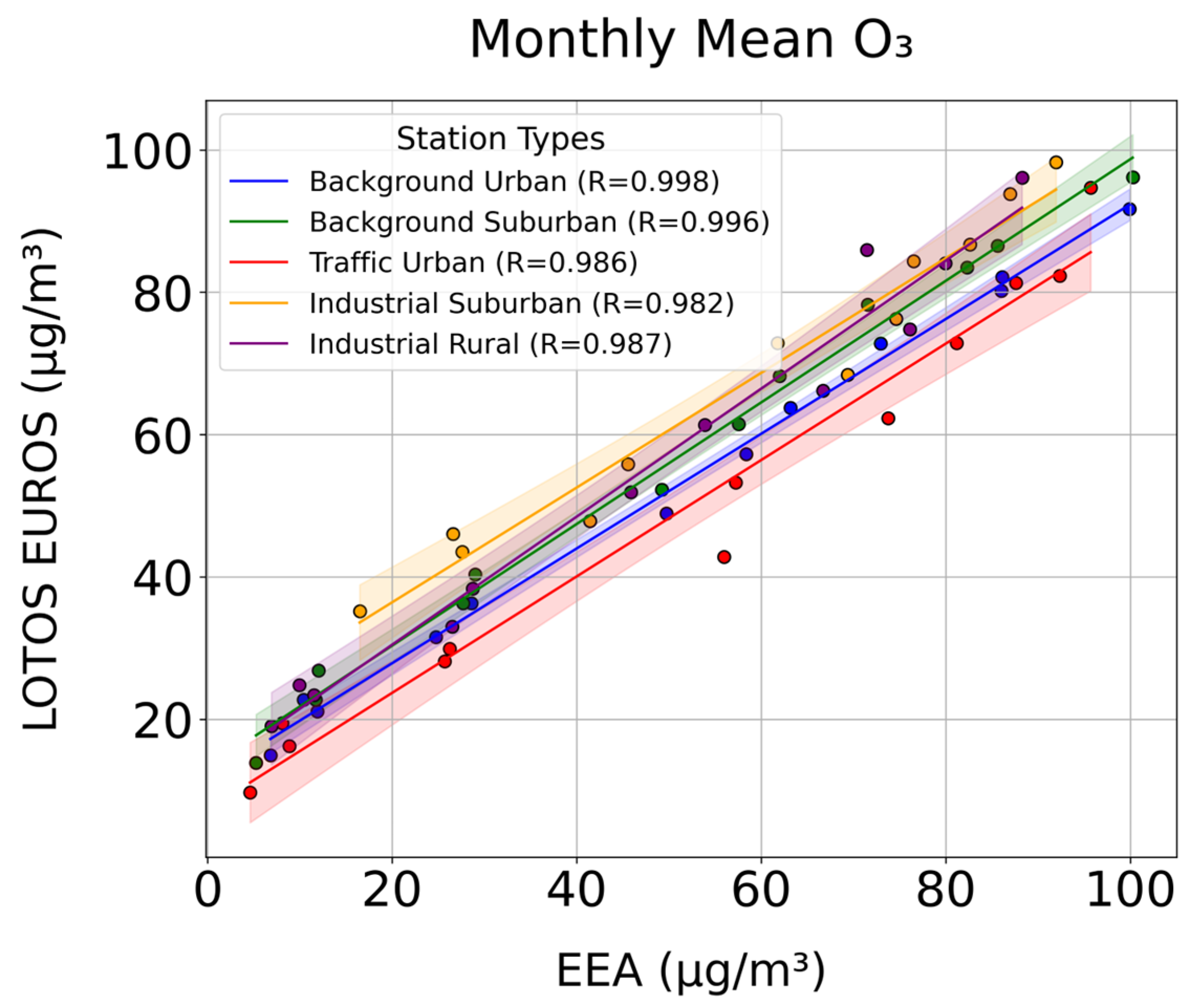
3.1.1. Monthly Mean Comparisons

In Figure 4, the monthly mean surface concentrations from the EEA in situ measurements (blue) and the LOTOS-EUROS model simulations (red) are presented for the traffic urban (a) and industrial suburban (b) stations. The data demonstrate that both lines exhibit a common seasonal variability. However, quantitative analysis reveals that LOTOS-EUROS consistently overestimates ozone concentrations in winter and more specifically in the months of October and November. Additionally, the EEA dataset (blue shading) exhibits a broader range of variability compared to the LOTOS-EUROS dataset (red shading), particularly during the warmer months. This indicates that the actual measurements display greater variability than the model predictions. The scatter plot comparison of the monthly mean in situ measurements and LOTOS-EUROS simulations is presented in Figure 5 for all station types. All correlation coefficients are consistently high (R > 0.98), indicating that the LOTOS-EUROS model is highly effective at capturing the temporal patterns and overall seasonal trends of ozone concentrations, as documented in [18]. The high R-values ascribe a remarkably strong agreement with the recorded concentrations by the ground-based stations. The model is highly effective in representing the measured ozone concentrations on a monthly basis and can be a reliable tool for predicting or estimating ozone concentrations, as it closely tracks the actual measurement.

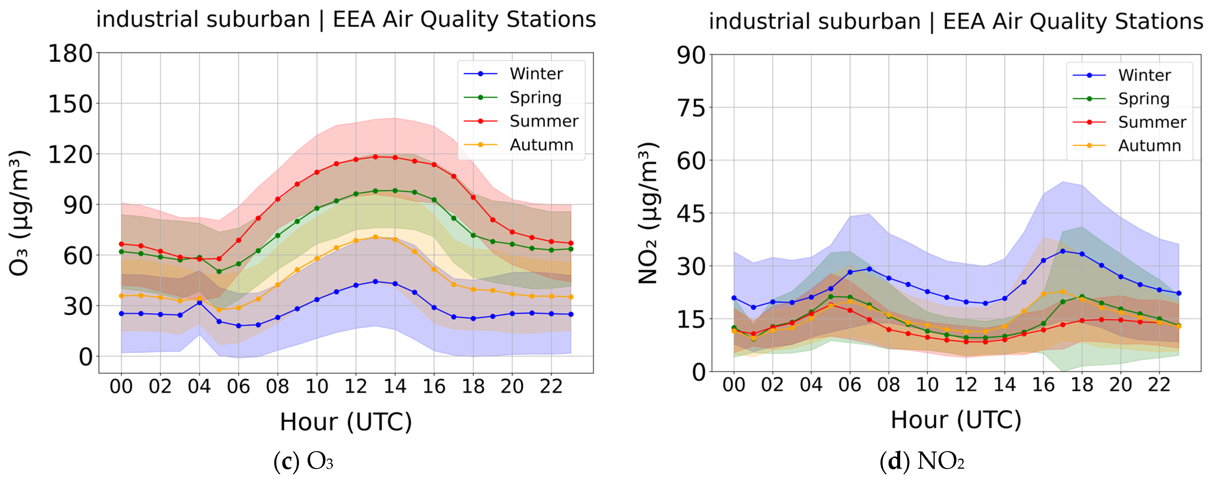
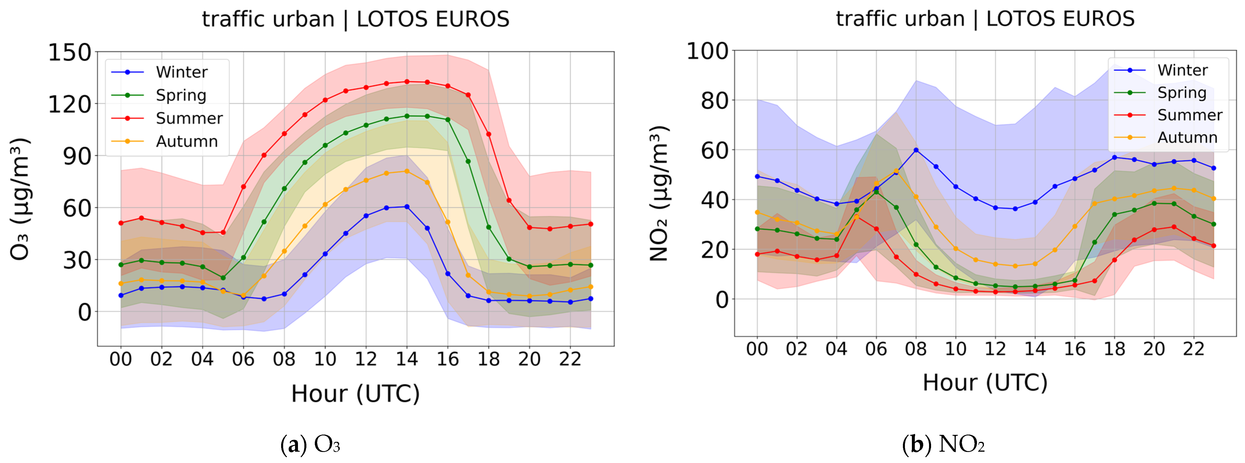
3.1.2. Seasonal and Diurnal Comparisons

After assessing seasonal variability, the diurnal variability per season is examined in this sub-section before proceeding to a direct comparison between surface observations and simulations.
The diurnal variability of traffic urban (a,b) and industrial suburban (c,d) stations is shown on a seasonal basis in Figure 6 for the EEA O3 (a,c) and NO2 (b,d) measurements. A pronounced diurnal variation in surface O3 is seen, with the highest levels appearing during summer months, followed by spring, autumn, and finally winter, where ozone formation is significantly reduced. The highest concentration of ozone falls within the range of ~120–140 µg/m3, and it is observed at midday between 13:00 and 14:00 UTC when the strength of sunlight is the greatest. On the other hand, the lowest concentration ranging between ~4 and 14 µg/m3 is recorded between 4:00 and 6:00 UTC. A comparative analysis of the various station types indicates that the industrial suburban stations exhibit the highest peaks and lows in ozone concentrations during the colder seasons, specifically winter (peak = 44.23 μg/m3 and minimum = 18.04 μg/m3) and autumn (peak = 70.64 μg/m3 and minimum = 27.45 μg/m3). A relevant study on the analysis of air pollution and climate at a background site in the Po Valley [11] showed comparable diurnal patterns for O3 and implied that the summer diurnal pattern is significantly influenced by the enhanced dispersion induced by the warm summer weather that is typical of the Po Valley.
A distinct diurnal pattern is observed for NO2 levels over the traffic urban station (Figure 6b), with two peaks in NO2 concentration: one in the morning, occurring around 5:00 to 6:00 UTC, and the other during the evening rush hour between 18:00 and 19:00 UTC, indicating that traffic emissions have a significant impact during these times. It is noteworthy that the summertime peak occurs earlier in the morning than it does during the winter months. This phenomenon is attributed to the onset of photochemistry, which commences at an earlier time due to the earlier rising of the sun. The identified NO2 behavior is observed in all five types of stations across all seasons examined in this study, including the industrial suburban case (Figure 6d). The industrial rural stations () are the exception, exhibiting less pronounced diurnal fluctuations, implying that industrial zones tend to have more consistent emissions than the pulsed traffic emissions observed in urban areas. The traffic urban station exhibits the most pronounced peaks for NO2, displaying peak and minimum concentrations approximately 1.5 to 2 times larger than those observed at other station types for all seasons. In particular, during the winter season, the levels reach ~50 µg/m3 at 07:00 UTC (early morning) and ~60 µg/m3 at 18:00 UTC (late afternoon). Conversely, in the winter period, the background suburban stations exhibit the lowest minimum value (~3 μg/m3), in stark contrast to the other station types, which display low values within the range of ~18–35 μg/m3. The presented NO2 diurnal cycle is well in line with the findings of [24], which conclude that the double-peaked pattern observed in winter is due to traffic emissions during the rush hour periods, with the evening peak extended longer than the morning peak partly due to higher nighttime atmospheric stability as well as decreased photochemical destruction due to insufficient sunlight.
The corresponding seasonal diurnal timeseries, derived from the LOTOS-EUROS simulations, are presented in Figure 7 and reveal a discernible seasonal trend for ozone (a,c) analogous to that observed in Figure 6. The highest O3 concentrations, around 125–132 μg/m3, are observed during the summer months (red line), reaching their peak at ~14:00 UTC, while the lowest concentrations (~5–32 μg/m3) are observed in wintertime (blue). It is noteworthy that the industrial suburban stations exhibit the highest minimum concentrations, which are approximately two to three times higher than those observed at other station types across all seasons. On the contrary, the traffic urban station consistently exhibits the lowest minimum concentrations. A review of the NO2 diurnal variability (Figure 7b,d) reveals a similar distinct seasonal pattern across all station types to that observed in the EEA NO2 case study. The highest concentrations are observed during winter (~30–59 μg/m3) at ~7:00 UTC, and the lowest concentration levels are observed at ~13:00 UTC throughout the summer within the range of ~1–3 μg/m3. Among station types, it is found that the traffic urban station shows the greatest peak and minimum concentrations of NO2, reaching levels up to twice those observed in other stations. In contrast, the industrial suburban stations exhibit the lowest diurnal variability (Figure 7d).
The correlation between the seasonal urban variability measured by the in situ stations and the LOTOS-EUROS simulations datasets is highly significant, with correlation coefficients ranging between 0.83 and 0.98 and p-values near zero (Table 2), while the diurnal cycle is accurately represented by the model. Even though the wintertime correlations are the highest for all types of stations, the LOTOS-EUROS simulations result in higher morning peaks for both O3 and NO2. This fact merits further investigation since it was established that the surface levels were not influenced by probable intrusions from the free troposphere into the planetary boundary layer, which might have possibly enhanced the surface concentrations. In summary, the LOTOS-EUROS model simulations show a remarkable ability to capture the diurnal cycles of ozone across different station types and seasons and agree well with the in situ measurements.

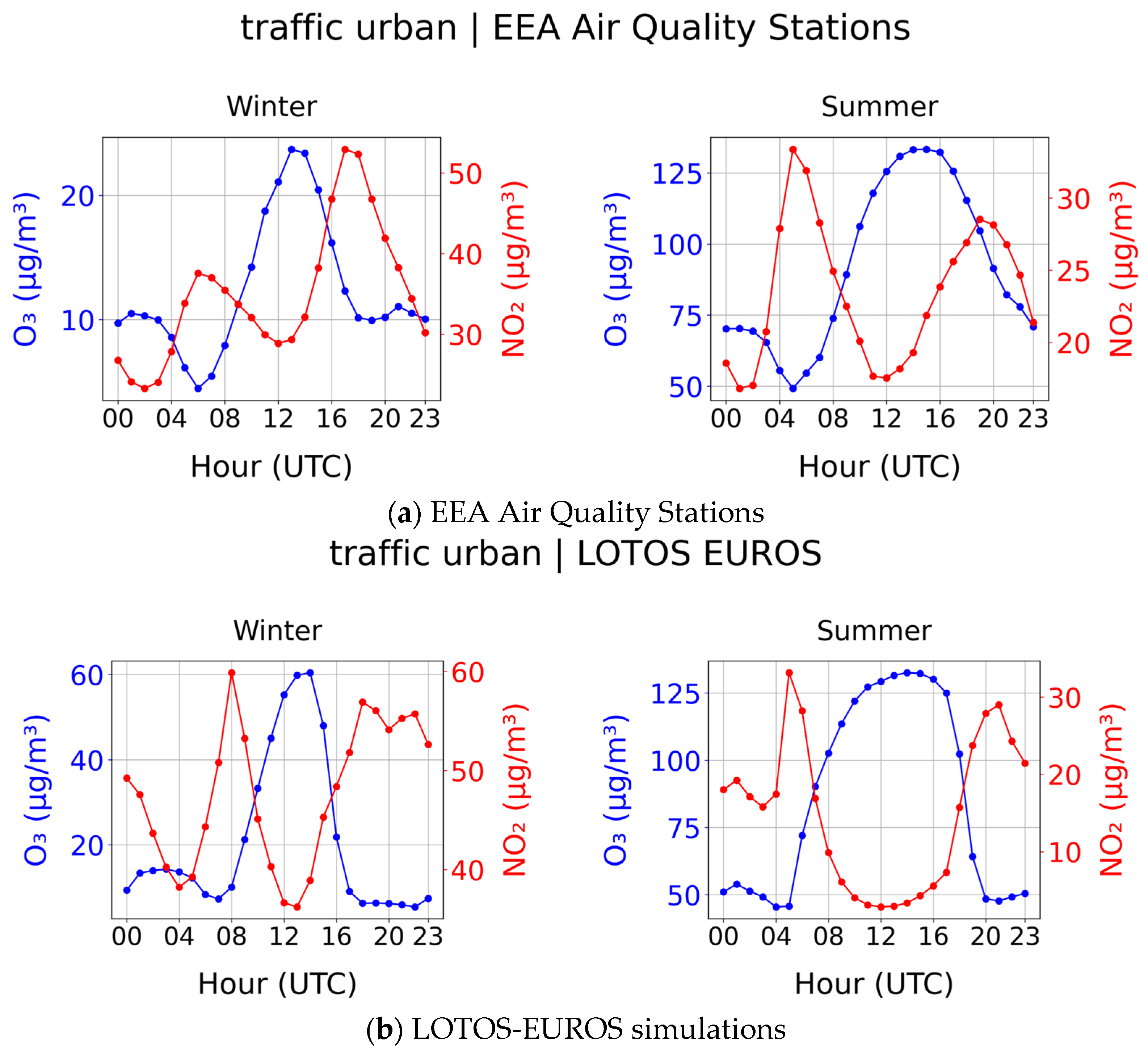
3.1.3. Co-Variability of Ozone and Nitrogen Dioxide Levels

This sub-section aims to provide an extensive analysis of the co-variability between O3 and NO2. In all station types for the EEA measurements, there is an inverse relationship between ozone and nitrogen dioxide, particularly during daylight hours. The measurements of the traffic urban station (Figure 8a) exhibit the greatest diurnal fluctuations in NO2 concentrations due to traffic-related emissions, while industrial and background stations report more uniform pollutants levels throughout the day. The LOTOS-EUROS simulations also demonstrate an inverse correlation between O3 and NO2, which is most pronounced during summer midday (Figure 8b). The inverse relationship between O3 and NO2 follows a study conducted in the urban background atmosphere of Nanjing, East China [50], which demonstrated that during the summer months, the increased intensity of sunlight and elevated temperatures result in elevated rates of NO2 photolysis, consequently leading to a more pronounced formation of ozone. This is attributed to the elevated midday O3 levels observed during the summer season in comparison to other seasons. In winter, the reduction in sunlight and temperatures results in a decrease in photochemical activity, leading to lower ozone levels and higher NO2 concentrations. The conditions are more favorable for the decreased photolytic breakdown of NO2 in winter. Furthermore, ref. [50] emphasized the pivotal role of nitrogen oxide (NO) in reducing ozone levels through the titration effect, whereby NO reacts with O3 to form NO2, thereby depleting ozone. This effect is particularly evident during the early morning and late evening hours, when NO concentrations are elevated due to traffic emissions and reduced photolytic activity. Consequently, lower O3 levels are observed during these periods.
To further investigate their correlation, Figure 9 presents a scatterplot of monthly mean O3 and NO2 for all station types. As can be seen, the EEA measurements (Figure 9a) exhibit a pervasive negative correlation (R) across all station types, with R values ranging from −0.76 to −0.88. The LOTOS-EUROS simulations (Figure 9b) also demonstrate an inverse relationship between O3 and NO2, albeit with higher correlation coefficients (R > −0.96), indicating a stronger covariance of the simulations. This is to be expected given that the model’s spatial resolution is inherently limited by the resolution of the meteorological and emission input data. This constraint is particularly evident in traffic urban stations, where the model struggles to capture sharp concentration gradients and localized emission dynamics. Consequently, the simulated O3 and NO2 fields appear more smoothed, resulting in a stronger inverse linear relationship compared to the measured data.

4. Discussion

An air quality assessment, at a European scale, is traditionally performed using the in situ air quality monitoring measurements reported officially to the EEA database. In recent years, chemical transport modeling has emerged as a dependable alternative which can bridge the spatial locations that the deployment of in situ stations cannot cover, which leaves a large part of Europe under-represented in the annual reviews on the state of European air quality. Increasingly, chemical transport models are gaining ground in determining air quality, as evidenced by their extensive application and validation in numerous recent studies.
Our study, which integrates ground-based EEA measurements with LOTOS-EUROS CTM simulations to assess ozone levels over the Po Valley, fits within a growing body of work that combines observational data with chemical transport models to better understand regional air quality. For instance, ref. [51] employed WRF-Chem to evaluate ozone concentrations across Europe, similarly emphasizing the value of coupling models with empirical data. In a different context, ref. [52] demonstrated this integration through a hybrid approach in Montreal by using kriging with an external drift and Bayesian maximum entropy models to estimate ozone exposure, an effort that, like ours, aimed to improve the spatial resolution in ozone assessments. One of the key model behaviors observed in our work, namely the overestimation of ozone during morning peaks, echoes findings by [53], which noted comparable biases in the MACC reanalysis for Europe, pointing to persistent challenges in resolving diurnal ozone patterns accurately. Additionally, our identification of a strong inverse correlation between ozone and nitrogen dioxide levels aligns closely with the results of [54], whose spatiotemporal modeling in Montreal similarly underscored the complex interplay between these two pollutants. Finally, our use of the LOTOS-EUROS model shares conceptual ground with the work of [55], which applied the CHIMERE model to examine how varying spatial resolution affects ozone simulations, reinforcing the critical role that model configuration plays in capturing local air quality dynamics.

5. Conclusions

In this study, the air quality over the Po Valley in Northern Italy for the year 2022 was investigated using the surface concentrations of O3 and NO2 as air quality indicators. For this purpose, ground-based in situ measurements from EEA air quality stations as well as chemical transport simulations from the LOTOS-EUROS CTM were utilized. The in situ measurements are analyzed in detail in this work to act as the “ground truth” for the assessment of the capability of the CTM to describe accurately the air quality levels of the region. In that respect, our main conclusions can be summarized below:
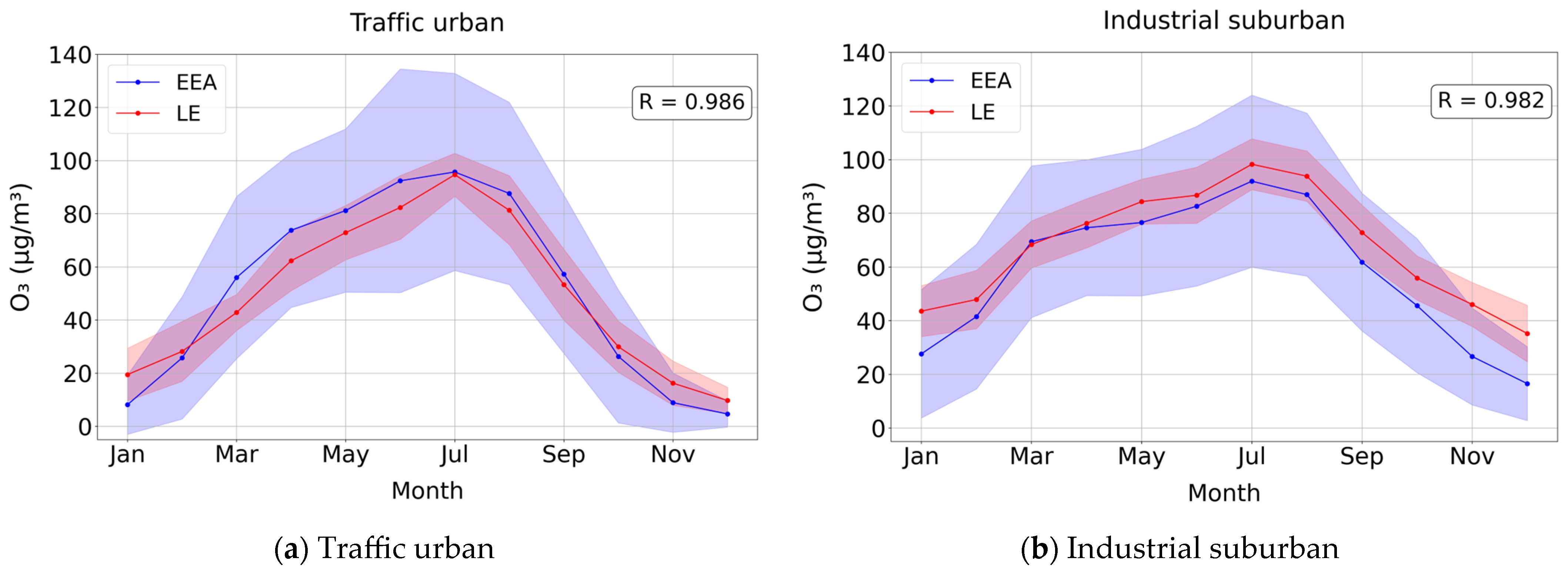
  • LOTOS-EUROS CTM simulations showed a strong correlation with EEA measurements (R > 0.98) on a monthly mean basis and displayed R values between 0.83 and 0.98 on a seasonal diurnal temporal scale, indicating that the LOTOS-EUROS model is highly effective at capturing the spatiotemporal temporal patterns and overall seasonal trends of ozone concentrations.
  • The inverse correlation between ozone and nitrogen dioxide surface levels reported by the EEA in situ measurements reports high R values from −0.76 to −0.88, while the CTM, due to the spatial resolution of the simulations which prevents the identification of local effects, reports higher correlations of −0.96 to −0.99.
  • The consistent overestimation of ozone concentrations during their morning peak levels in January and February 2022 identified in this work remains a point for further investigation.
With respect to the ozone-related air quality assessment based on the EEA in situ stations, it was shown that all 28 stations studied in this work exceeded the EU ozone limit for an 8 h average of 120 μg/m3 for over 33 days and the WHO limit of 100 μg/m3 for more than 78 days, with the highest exceedances occurring in urban and suburban areas (Figure 10a). Displaying a similar spatial pattern, albeit in some cases with a higher number of days reporting exceedances, the LOTOS-EUROS CTM simulations (Figure 10b) can provide a suitable addition to the assessment of air quality in the region.
In summary, the results of the EEA measurements and LOTOS-EUROS simulations were consistent with the seasonal variation and diurnal patterns documented in the literature for O3 and NO2. The model effectively mirrors the EEA observed ozone concentrations on a monthly scale, and its simulations may serve as a trustworthy tool for forecasting or estimating ozone levels, as they align closely with the ground-based in situ measurements.
Looking forward, future work could explore integrating higher-resolution simulations or hybrid approaches that combine CTMs with data assimilation techniques or machine learning models, which may help address localized discrepancies. Additionally, ongoing refinement of CTMs with newer in situ measurements and expanding their validation across other regions in Europe could strengthen their application in large-scale monitoring efforts. From a policy perspective, our findings reinforce the necessity for supplementary assessment tools like CTMs to complement the current EEA network, especially in regions with sparse coverage. This dual-source strategy could support more equitable and comprehensive air quality reporting across Europe while also enabling more informed mitigation planning in urban hotspots like the Po Valley. Ultimately, such approaches could aid EU policy-makers in tracking compliance with air quality standards and shaping evidence-based strategies to reduce public health impacts.

Author Contributions

Conceptualization, M.-E.K., K.G. and D.B.; methodology, M.-E.K. and A.P.; software, S.M.; validation, S.M. and A.P.; formal analysis, S.M.; data curation, S.M. and A.P.; visualization, S.M.; writing—original draft preparation, S.M., A.P. and M.-E.K.; writing—review and editing, all authors; supervision, K.G. and D.B. All authors have read and agreed to the published version of the manuscript.

Funding

This research received no external funding.

Data Availability Statement

The European Environment Agency (EEA) air quality monitoring station datasets are publicly available from https://eeadmz1-downloads-webapp.azurewebsites.net/, last accessed on 20 December 2024. The LOTOS-EUROS v2.3 is an open-source chemical transport model (CTM) available from https://airqualitymodeling.tno.nl/lotos-euros/open-source-version/, last accessed on 20 December 2024. The LOTOS-EUROS simulations shown in this article are available upon request from A.P.

Acknowledgments

Results presented in this work have been produced using the Aristotle University of Thessaloniki (AUTh) High-Performance Computing Infrastructure and Resources. The authors would like to acknowledge the support provided by the IT Center of the Aristotle University of Thessaloniki (AUTh) throughout the progress of this research work.

Conflicts of Interest

The authors declare no conflicts of interest.

Appendix A

Table A1. Selected EEA air quality monitoring stations.
Sampling Point Name/Locality CityStation Type
SPO.IT0705AVerziereMilanoTraffic urban
SPO.IT0706AVia Palermo AngoloPioltelloBackground urban
SPO.IT0804AParco CittadellaParmaBackground urban
SPO.IT0842AV. villaCremonaIndustrial rural
SPO.IT0892AGiardini MargheritaBolognaBackground urban
SPO.IT0912AVia FolpertiPaviaBackground urban
SPO.IT0940AVia AmendolaReggio N. EmiliaBackground urban
SPO.IT1144AVia PilalungaSavonaIndustrial suburban
SPO.IT1459AAccamBusto ArsizioBackground suburban
SPO.IT1590ALancieridi NovaraTrevisoBackground urban
SPO.IT1650ASantuarioSaronnoBackground urban
SPO.IT1692APascalMilanBackground urban
SPO.IT1737AVilaggio SerenoBresciaBackground urban
SPO.IT1739AFatebene fratelliCremonaBackground urban
SPO.IT1743AMachiavelliMonzaBackground urban
SPO.IT1746AVia VignePaviaIndustrial rural
SPO.IT1771AParco FerrariModenaBackground urban
SPO.IT1830ASpalto MarengoAlessandriaBackground urban
SPO.IT1871AVia BragadineEsteIndustrial suburban
SPO.IT1877ARubinoTorinoBackground urban
SPO.IT1918AVilla FulviaFerraraBackground urban
SPO.IT1975AParco MontecuccoPiacenzaBackground urban
SPO.IT2063AVia Cesare BattistiCremonaIndustrial rural
SPO.IT2075AChiariniBolognaBackground suburban
SPO.IT2098AMirabellinoMonzaBackground suburban
SPO.IT2168AViale Augusto MontiTorinoBackground urban
SPO.IT2232AEdisonCormanoBackground urban
SPO.IT2282AArpaNovaraBackground urban
Figure A1. Days exceeding the EU Air Quality Standards for max 8 h mean ozone concentration by city population.
Remotesensing 17 01794 g0a1
Figure A2. Days exceeding the WHO air quality guideline for 8 h mean ozone concentration by city population.
Remotesensing 17 01794 g0a2

References

  1. Sharma, A.K.; Sharma, M.; Sharma, A.K.; Sharma, M.; Sharma, M. Mapping the impact of environmental pollutants on human health and environment: A systematic review and meta-analysis. J. Geochem. Explor. 2023, 255, 107325. [Google Scholar] [CrossRef]
  2. Husain, L.; Coffey, P.E.; Meyers, R.E.; Cederwall, R.T. Ozone transport from stratosphere to troposphere. Geophys. Res. Lett. 1977, 4, 363–365. [Google Scholar] [CrossRef]
  3. Stohl, A.; Trickl, T. Long-Range Transport of Ozone from the North American Boundary Layer to Europe: Observations and Model Results. In Air Pollution Modeling and Its Application XIV; Springer: Boston, MA, USA, 2006; pp. 257–266. [Google Scholar] [CrossRef]
  4. Crutzen, P.J. The Role of NO and NO2 in the Chemistry of the Troposphere and Stratosphere. Annu. Rev. Earth Planet. Sci. 1979, 7, 443–472. [Google Scholar] [CrossRef]
  5. Jiang, X.; Cheng, X.; Liu, J.; Chen, Z.; Wang, H.; Deng, H.; Hu, J.; Jiang, Y.; Yang, M.; Gai, C.; et al. Comparison of Surface Ozone Variability in Mountainous Forest Areas and Lowland Urban Areas in Southeast China. Atmosphere 2024, 15, 519. [Google Scholar] [CrossRef]
  6. Lakshmi, K.A.K.; Nishanth, T.; Kumar, S.; Valsaraj, K.T. A Comprehensive Review of Surface Ozone Variations in Several Indian Hotspots. Atmosphere 2024, 15, 852. [Google Scholar] [CrossRef]
  7. Badr, O.; Probert, S.D. Oxides of nitrogen in the Earth’s atmosphere: Trends, sources, sinks and environmental impacts. Appl. Energy 1993, 46, 1–67. [Google Scholar] [CrossRef]
  8. Monks, P.S.; Archibald, A.T.; Colette, A.; Cooper, O.; Coyle, M.; Derwent, R.; Fowler, D.; Granier, C.; Law, K.S.; Mills, G.E.; et al. Tropospheric ozone and its precursors from the urban to the global scale from air quality to short-lived climate forcer. Atmos. Chem. Phys. 2015, 15, 8889–8973. [Google Scholar] [CrossRef]
  9. Koukouli, M.-E.; Pseftogkas, A.; Karagkiozidis, D.; Skoulidou, I.; Drosoglou, T.; Balis, D.; Bais, A.F.; Melas, D.; Hatzianastassiou, N. Air Quality in Two Northern Greek Cities Revealed by Their Tropospheric NO2 Levels. Atmosphere 2022, 13, 840. [Google Scholar] [CrossRef]
  10. Beirle, S.; Platt, U.; Wenig, M.; Wagner, T. Weekly cycle of NO2 by GOME measurements: A signature of anthropogenic sources. Atmos. Chem. Phys. 2003, 3, 2225–2232. [Google Scholar] [CrossRef]
  11. Jenkin, M.E.; Clemitshaw, K.C. Chapter 11 Ozone and other secondary photochemical pollutants: Chemical processes governing their formation in the planetary boundary layer. Dev. Environ. Sci. 2002, 1, 285–338. [Google Scholar] [CrossRef]
  12. Wayne, R.P.; Barnes, I.; Biggs, P.; Burrows, J.P.; Canosa-Mas, C.E.; Hjorth, J.; Le Bras, G.; Moortgat, G.K.; Perner, D.; Poulet, G.; et al. The nitrate radical: Physics, chemistry, and the atmosphere. Atmos. Environ. Part A. Gen. Top. 1991, 25, 1–203. [Google Scholar] [CrossRef]
  13. Atkinson, R.; Arey, J. Gas-phase tropospheric chemistry of biogenic volatile organic compounds: A review. Atmos. Environ. 2003, 37, 197–219. [Google Scholar] [CrossRef]
  14. Stull, R.B. An Introduction to Boundary Layer Meteorology; Springer: New York, NY, USA, 2012. [Google Scholar]
  15. Jacob, D.J. Introduction to Atmospheric Chemistry; Princeton University Press: Princeton, NJ, USA, 1999. [Google Scholar]
  16. Po Valley. Available online: https://geography.name/po-valley/ (accessed on 10 May 2025).
  17. Pivato, A.; Pegoraro, L.; Masiol, M.; Bortolazzo, E.; Bonato, T.; Formenton, G.; Cappai, G.; Beggio, G.; Giancristofaro, R.A. Long time series analysis of air quality data in the Veneto region (Northern Italy) to support environmental policies. Atmos. Environ. 2023, 298, 119610. [Google Scholar] [CrossRef]
  18. Masiol, M.; Squizzato, S.; Formenton, G.; Harrison, R.M.; Agostinelli, C. Air quality across a European hotspot: Spatial gradients, seasonality, diurnal cycles and trends in the Veneto region, NE Italy. Sci. Total Environ. 2017, 576, 210–224. [Google Scholar] [CrossRef]
  19. European Commission. Air Quality. Available online: https://environment.ec.europa.eu/topics/air/air-quality_en (accessed on 10 May 2025).
  20. World Health Organization. What Are the WHO Air Quality Guidelines? 2021. Available online: https://www.who.int/news-room/feature-stories/detail/what-are-the-who-air-quality-guidelines (accessed on 10 May 2025).
  21. Benassi, A.; Dalan, F.; Gnocchi, A.; Maffeis, G.; Malvasi, G.; Liguori, F.; Pernigotti, D.; Pillon, S.; Sansone, M.; Susanetti, L. A one-year application of the Veneto air quality modelling system: Regional concentrations and deposition on Venice lagoon. Int. J. Environ. Pollut. 2011, 44, 32. [Google Scholar] [CrossRef]
  22. Martilli, A.; Neftel, A.; Favaro, G.; Kirchner, F.; Sillman, S.; Clappier, A. Simulation of the ozone formation in the northern part of the Po Valley. J. Geophys. Res. 2002, 107, 8195. [Google Scholar] [CrossRef]
  23. Maurizi, A.; Russo, F.; Tampieri, F. Local vs. external contribution to the budget of pollutants in the Po Valley (Italy) hot spot. Sci. Total Environ. 2013, 458–460, 459–465. [Google Scholar] [CrossRef]
  24. Bigi, A.; Ghermandi, G.; Harrison, R.M. Analysis of the air pollution climate at a background site in the Po valley. J. Environ. Monit. 2012, 14, 552–563. [Google Scholar] [CrossRef]
  25. Spirig, C.; Neftel, A.; Kleinman, L.I.; Hjorth, J. NOx versus VOC limitation of O3 production in the Po valley: Local and integrated view based on observations. J. Geophys. Res. 2002, 107, 8191. [Google Scholar] [CrossRef]
  26. Kaiser, J.; Wolfe, G.M.; Bohn, B.; Broch, S.; Fuchs, H.; Ganzeveld, L.N.; Gomm, S.; Häseler, R.; Hofzumahaus, A.; Holland, F.; et al. Evidence for an unidentified non-photochemical ground-level source of formaldehyde in the Po Valley with potential implications for ozone production. Atmos. Chem. Phys. 2015, 15, 1289–1298. [Google Scholar] [CrossRef]
  27. Thunis, P.; Triacchini, G.; White, L.; Maffeis, G.; Volta, M. Air Pollution and Emission Reductions over the Po-Valley: Air Quality Modelling and Integrated Assessment. 18th World IMACS/MODSIM. 2009. Available online: https://mssanz.org.au/modsim09/F10/thunis.pdf (accessed on 15 December 2024).
  28. Cai, M.; Ye, C.; Yuan, B.; Huang, S.; Zheng, E.; Yang, S.; Wang, Z.; Lin, Y.; Li, T.; Hu, W.; et al. Enhanced daytime secondary aerosol formation driven by gas–particle partitioning in downwind urban plumes. Atmos. Chem. Phys. 2024, 24, 13065–13079. [Google Scholar] [CrossRef]
  29. Zhang, G.; Yu, X.; Yin, H.; Feng, C.; Ma, C.; Sun, S.; Cheng, H.; Wang, S.; Shang, K.; Liu, X. Heatwave-amplified atmospheric oxidation in a multi-province border area in Xuzhou, China. Front. Environ. Sci. 2024, 12. [Google Scholar] [CrossRef]
  30. Manders, A.M.M.; Builtjes, P.J.H.; Curier, L.; van der Gon, H.A.C.D.; Hendriks, C.; Jonkers, S.; Kranenburg, R.; Kuenen, J.J.P.; Segers, A.J.; Timmermans, R.M.A. Curriculum vitae of the LOTOS–EUROS (v2.0) chemistry transport model. Geosci. Model Dev. 2017, 10, 4145–4173. [Google Scholar] [CrossRef]
  31. Topographic Maps. Po Valley Topographic Map, Elevation, Terrain. Available online: https://en-us.topographic-map.com/map-6ffntf/Po-Valley/ (accessed on 15 December 2024).
  32. Zhu, T.; Melamed, M.L.; Parrish, D.; Gllardo Klenner, L.; Lawrence, M.; Konare, A.; Liousse, C. (Eds.) WMO/IGAC Impacts of Megacities on Air Pollution and Climate; World Meteorological Organization: Geneva, Switzerland, 2012; 299p, ISBN 978-0-9882867-0-2. [Google Scholar]
  33. Hakim, Z.M.; Archer-Nicholls, S.; Beig, G.; Folberth, G.A.; Sudo, K.; Abraham, N.L.; Ghude, S.D.; Henze, D.K.; Archibald, A.T. Evaluation of tropospheric ozone and ozone precursors in simulations from the HTAPII and CCMI model intercomparisons—A focus on the Indian subcontinent. Atmos. Chem. Phys. 2019, 19, 6437–6458. [Google Scholar] [CrossRef]
  34. Caserini, S.; Giani, P.; Cacciamani, C.; Ozgen, S.; Lonati, G. Influence of climate change on the frequency of daytime temperature inversions and stagnation events in the Po Valley: Historical trend and future projections. Atmos. Res. 2017, 184, 15–23. [Google Scholar] [CrossRef]
  35. Masiol, M.; Agostinelli, C.; Formenton, G.; Tarabotti, E.; Pavoni, B. Thirteen years of air pollution hourly monitoring in a large city: Potential sources, trends, cycles and effects of car-free days. Sci. Total Environ. 2014, 494–495, 84–96. [Google Scholar] [CrossRef]
  36. Bigi, A.; Ghermandi, G. Long-term trend and variability of atmospheric PM10 concentration in the Po Valley. Atmos. Chem. Phys. 2014, 14, 4895–4907. [Google Scholar] [CrossRef]
  37. Serio, C.; Masiello, G.; Cersosimo, A. NO2 pollution over selected cities in the Po valley in 2018–2021 and its possible effects on boosting COVID-19 deaths. Heliyon 2022, 8, e09978. [Google Scholar] [CrossRef]
  38. Schaap, M.; Timmermans, R.M.A.; Roemer, M.; Boersen, G.A.C.; Builtjes, P.J.H.; Sauter, F.J.; Velders, G.J.M.; Beck, J.P. The LOTOS–EUROS model: Description, validation and latest developments. Int. J. Environ. Pollut. 2008, 32, 270–290. [Google Scholar] [CrossRef]
  39. Skoulidou, I.; Koukouli, M.-E.; Manders, A.; Segers, A.; Karagkiozidis, D.; Gratsea, M.; Balis, D.; Bais, A.; Gerasopoulos, E.; Stavrakou, T.; et al. Evaluation of the LOTOS-EUROS NO2 simulations using ground-based measurements and S5P/TROPOMI observations over Greece. Atmos. Chem. Phys. 2021, 21, 5269–5288. [Google Scholar] [CrossRef]
  40. Pseftogkas, A.; Koukouli, M.-E.; Segers, A.; Manders, A.; van Geffen, J.; Balis, D.; Meleti, C.; Stavrakou, T.; Eskes, H. Comparison of S5P/TROPOMI Inferred NO2 Surface Concentrations with In Situ Measurements over Central Europe. Remote Sens. 2022, 14, 4886. [Google Scholar] [CrossRef]
  41. Escudero, M.; Segers, A.; Kranenburg, R.; Querol, X.; Alastuey, A.; Borge, R.; de la Paz, D.; Gangoiti, G.; Schaap, M. Analysis of summer O3 in the Madrid air basin with the LOTOS-EUROS chemical transport model. Atmos. Chem. Phys. 2019, 19, 14211–14232. [Google Scholar] [CrossRef]
  42. Curier, R.L.; Timmermans, R.; Calabretta-Jongen, S.; Eskes, H.; Segers, A.; Swart, D.; Schaap, M. Improving ozone forecasts over Europe by synergistic use of the LOTOS-EUROS chemical transport model and in-situ measurements. Atmos. Environ. 2012, 60, 217–226. [Google Scholar] [CrossRef]
  43. Hersbach, H.; Bell, B.; Berrisford, P.; Hirahara, S.; Horányi, A.; Muñoz-Sabater, J.; Nicolas, J.; Peubey, C.; Radu, R.; Schepers, D.; et al. The ERA5 global reanalysis. Q. J. R. Meteorol. Soc. 2020, 146, 1999–2049. [Google Scholar] [CrossRef]
  44. Kuenen, J.; Dellaert, S.; Visschedijk, A.; Jalkanen, J.-P.; Super, I.; van der Gon, H.D. CAMS-REG-v4: A state-of-the-art high-resolution European emission inventory for air quality modelling. Earth Syst. Sci. Data 2022, 14, 491–515. [Google Scholar] [CrossRef]
  45. van der Gon, H.D.; Gauss, M.; Granier, C.; Arellano, S.; Benedictow, A.; Darras, S.; Dellaert, S.; Guevara, M.; Jalkanen, J.-P.; Krueger, K.; et al. Copernicus Atmosphere CAMS2_61—Global and European Emission Inventories Documentation of CAMS Emission Inventory Products; Copernicus Atmosphere Monitoring Service: Reading, UK, 2023. [Google Scholar] [CrossRef]
  46. Lu, X.; Zhang, L.; Shen, L. Meteorology and Climate Influences on Tropospheric Ozone: A Review of Natural Sources, Chemistry, and Transport Patterns. Curr. Pollut. Rep. 2019, 5, 238–260. [Google Scholar] [CrossRef]
  47. Sullivan, J.T.; Apituley, A.; Mettig, N.; Kreher, K.; Knowland, K.E.; Allaart, M.; Piters, A.; Van Roozendael, M.; Veefkind, P.; Ziemke, J.R.; et al. Tropospheric and stratospheric ozone profiles during the 2019 TROpomi vaLIdation eXperiment (TROLIX-19). Atmos. Chem. Phys. 2022, 22, 11137–11153. [Google Scholar] [CrossRef]
  48. Nguyen, D.-H.; Lin, C.; Vu, C.-T.; Cheruiyot, N.K.; Nguyen, M.K.; Le, T.H.; Lukkhasorn, W.; Vo, T.-D.-H.; Bui, X.-T. Tropospheric ozone and NOx: A review of worldwide variation and meteorological influences. Environ. Technol. Innov. 2022, 28, 102809. [Google Scholar] [CrossRef]
  49. Wang, X.; Zhou, L.; Liu, Y.; Zhang, K.; Xiu, G. Investigating the photolysis of NO2 and influencing factors by using a DFT/TD-DFT method. Atmos. Environ. 2020, 230, 117559. [Google Scholar] [CrossRef]
  50. Jia, M.; Zhao, T.; Cheng, X.; Gong, S.; Zhang, X.; Tang, L.; Liu, D.; Wu, X.; Wang, L.; Chen, Y. Inverse Relations of PM2.5 and O3 in Air Compound Pollution between Cold and Hot Seasons over an Urban Area of East China. Atmosphere 2017, 8, 59. [Google Scholar] [CrossRef]
  51. Mar, K.A.; Ojha, N.; Pozzer, A.; Butler, T.M. Ozone air quality simulations with WRF-Chem (v3.5.1) over Europe: Model evaluation and chemical mechanism comparison. Geosci. Model Dev. 2016, 9, 3699–3728. [Google Scholar] [CrossRef]
  52. Adam-Poupart, A.; Brand, A.; Fournier, M.; Jerrett, M.; Smargiassi, A. Spatiotemporal Modeling of Ozone Levels in Quebec (Canada): A Comparison of Kriging, Land-Use Regression (LUR), and Combined Bayesian Maximum Entropy–LUR Approaches. Environ. Health Perspect. 2014, 122, 970–976. [Google Scholar] [CrossRef] [PubMed]
  53. Katragkou, E.; Zanis, P.; Tsikerdekis, A.; Kapsomenakis, J.; Melas, D.; Eskes, H.; Flemming, J.; Huijnen, V.; Inness, A.; Schultz, M.G.; et al. Evaluation of near-surface ozone over Europe from the MACC reanalysis. Geosci. Model Dev. 2015, 8, 2299–2314. [Google Scholar] [CrossRef]
  54. Buteau, S.; Hatzopoulou, M.; Crouse, D.L.; Smargiassi, A.; Burnett, R.T.; Logan, T.; Cavellin, L.D.; Goldberg, M.S. Comparison of spatiotemporal prediction models of daily exposure of individuals to ambient nitrogen dioxide and ozone in Montreal, Canada. Environ. Res. 2017, 156, 201–230. [Google Scholar] [CrossRef]
  55. Valari, M.; Menut, L. Does an Increase in Air Quality Models’ Resolution Bring Surface Ozone Concentrations Closer to Reality? J. Atmos. Ocean. Technol. 2008, 25, 1955–1968. [Google Scholar] [CrossRef]
Figure 1. Power plants and selected stations in Northern Italy. EEA stations are shown as colored circles, and power plants are shown as stars. The green shadow indicates the location of the Po Valley.
Remotesensing 17 01794 g001
Figure 2. Hourly (gray) and monthly (blue) mean EEA surface ozone (a,c) and nitrogen dioxide (b,d) concentrations (μg/m3) for the traffic urban and two industrial suburban stations over the Po Valley. The red line represents the 1-sigma error for the monthly mean concentration.
Remotesensing 17 01794 g002
Figure 3. Monthly mean LOTOS-EUROS surface concentrations of O3 in (a) winter and (c) summer and NO2 in (b) winter and (d) summer over Northern Italy. The locations of the EEA stations are given as blue circles and the coal and gas plants as black stars.
Remotesensing 17 01794 g003
Figure 4. Monthly mean surface EEA (blue) and LOTOS-EUROS (red) ozone concentrations (μg/m3) for the traffic urban and two industrial suburban stations over the Po Valley. The shaded areas represent the standard deviation of the monthly mean.
Remotesensing 17 01794 g004
Figure 5. Scatterplot of monthly mean surface EEA (x-axis) and LOTOS-EUROS (y-axis) ozone concentration (μg/m3) for all station types over the Po Valley. Shaded areas represent the 95% confidence intervals.
Remotesensing 17 01794 g005
Figure 6. Seasonal diurnal variability of EEA surface (a,c) ozone and (b,d) nitrogen dioxide concentrations (μg/m3) for one traffic urban and two industrial suburban stations over the Po Valley. The shaded areas represent the standard deviation of the hourly mean.
Remotesensing 17 01794 g006aRemotesensing 17 01794 g006b
Figure 7. Seasonal diurnal mean LOTOS-EUROS surface (a,c) ozone and (b,d) nitrogen dioxide concentrations (μg/m3) for one traffic urban and two industrial suburban stations over the Po Valley. The shaded areas represent the standard deviation of the hourly mean.
Remotesensing 17 01794 g007aRemotesensing 17 01794 g007b
Figure 8. Winter and summer diurnal mean surface O3 (blue) and NO2 (red) concentrations (μg/m3) for the traffic urban station from EEA measurements (a) and LOTOS-EUROS simulations (b) in central Milan.
Remotesensing 17 01794 g008
Figure 9. Scatterplot of monthly mean surface ozone and nitrogen dioxide concentrations (μg/m3) for all station types from (a) EEA stations and (b) LOTOS-EUROS simulations over the Po Valley. Shaded areas represent the 95% confidence intervals.
Remotesensing 17 01794 g009
Figure 10. Number of days exceeding the EU ozone 8 h limit for the locations of EEA in situ stations as reported by the ground-based measurements (a) and the LOTOS-EUROS simulations (b).
Remotesensing 17 01794 g010aRemotesensing 17 01794 g010b
Table 1. Annual mean O3 and NO2 concentrations (μg/m3) and the min and max monthly mean levels reported for different types of stations.
Station TypeAnnual O₃Monthly O3 Annual NO2Monthly NO2
(mean ± 1σ)maxmin(mean ± 1σ)maxmin
Background urban49.90 ± 32.8299.946.8225.76 ± 10.1442.8414.65
Background suburban49.52 ± 32.12100.275.2720.31 ± 7.3535.1812.74
Traffic urban51.46 ± 35.1195.724.6134.53 ± 10.1351.7121.16
Industrial suburban58.47 ± 25.9791.9616.5016.85 ± 5.5228.0111.19
Industrial rural47.18 ± 29.6488.286.9319.30 ± 4.7628.7313.50
Table 2. Seasonal correlation coefficients for all types of stations (p-value < < 0).
R Value
Station TypeWinterSpringSummerAutumn
Background urban0.980.960.940.97
Background suburban0.980.950.940.95
Traffic urban0.930.870.830.87
Industrial suburban0.930.950.980.97
Industrial rural0.940.960.960.97
Disclaimer/Publisher’s Note: The statements, opinions and data contained in all publications are solely those of the individual author(s) and contributor(s) and not of MDPI and/or the editor(s). MDPI and/or the editor(s) disclaim responsibility for any injury to people or property resulting from any ideas, methods, instructions or products referred to in the content.

