
Open and Free Sentinel-2 Mowing Event Data for Austria


Abstract

1. Introduction
- (1)
- What detection rate for mowing events can be expected from a fully automated, wall-to-wall, nationally applied approach independent from training data?
- (2)
- Is a pixel-based or a polygon-based application more suitable?
- (3)
- What is the detection delay overall and for the individual cut dates?
2. Materials
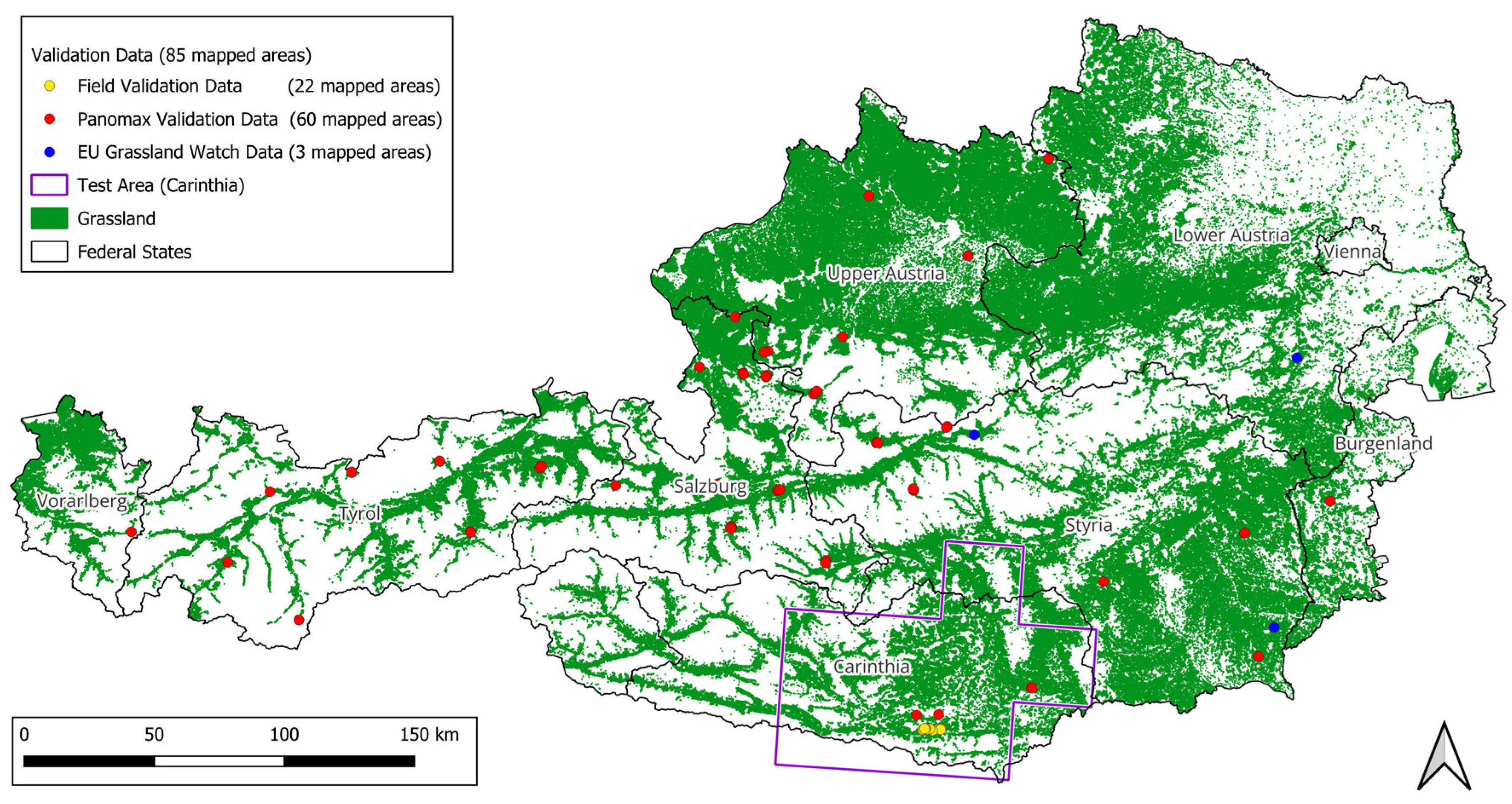
2.1. Study Area and Input Data
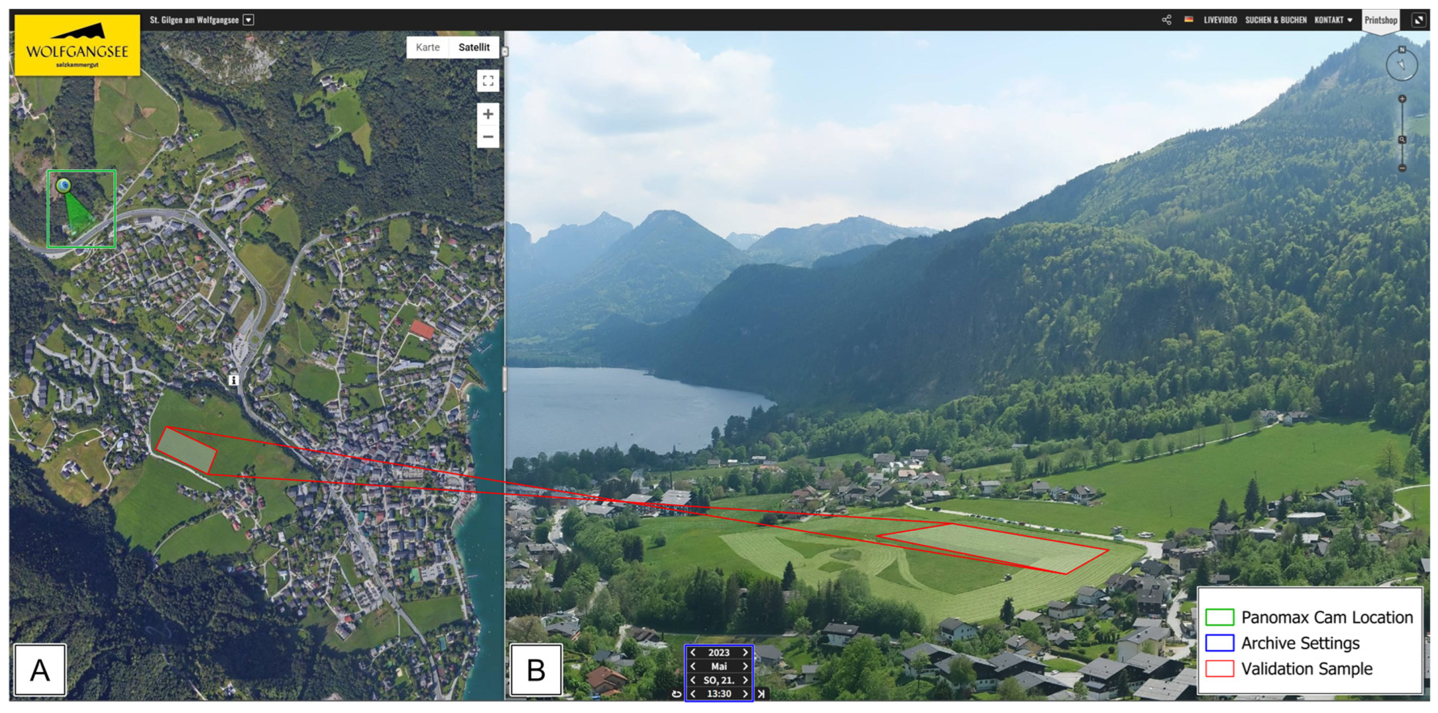
2.2. Validation Data
2.3. IACS Data for Comparison
3. Methods
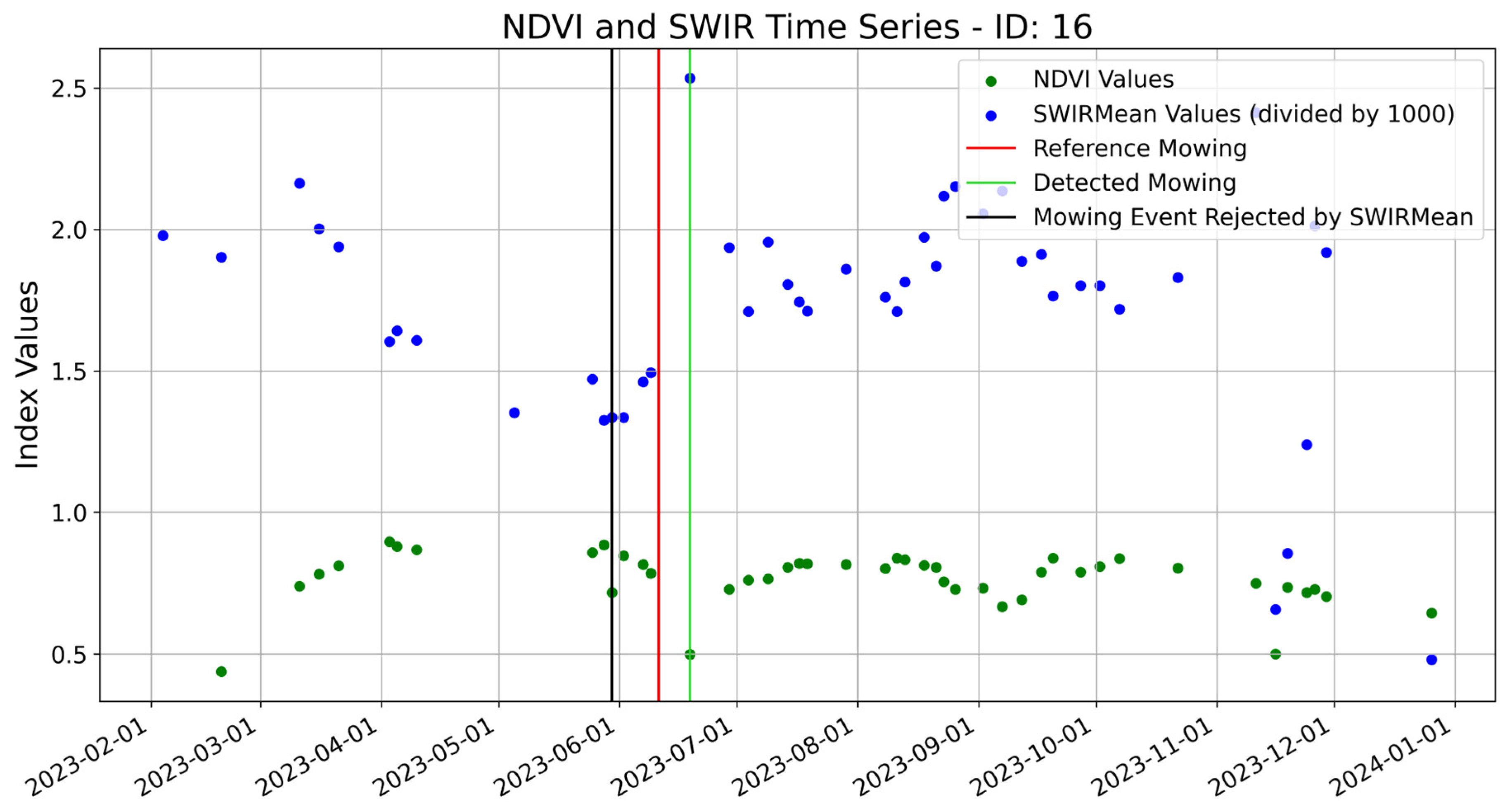
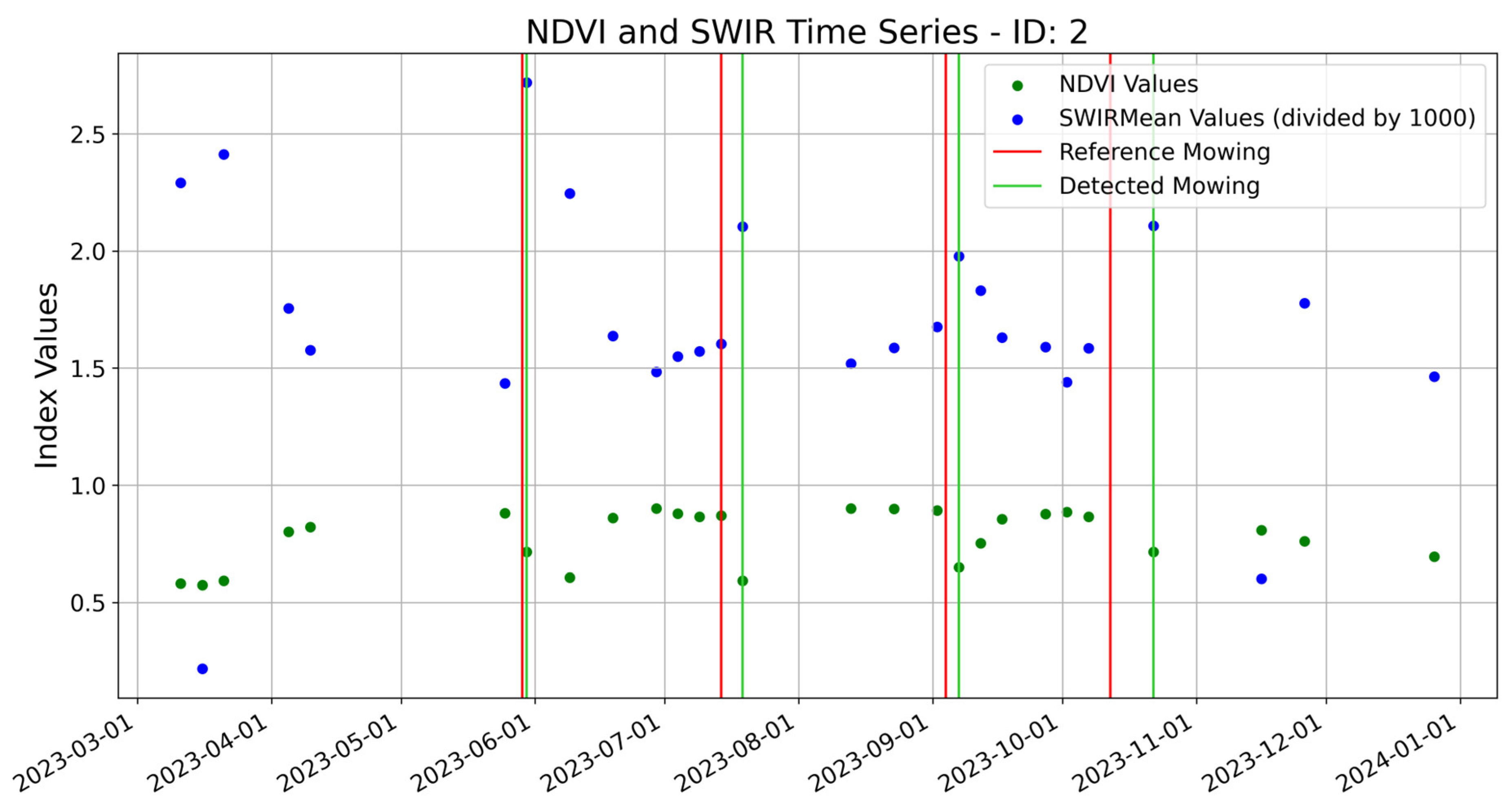
3.1. Mowing Event Detection Method
3.2. Validation Method
3.3. Method for Comparison with IACS
- -
- No mowing events were assumed for pastures (Hutweide).
- -
- One annual mowing event was assumed for mountain meadows (Bergmähder).
- -
- It was assumed that there was one mowing event per year for single-mown meadows (Mähwiese 1).
- -
- Two annual mowing events were assumed for mown meadows/pastures with two uses (Mähwiese 2).
- -
- It was assumed that mown meadows/pastures with three or more uses (Mähwiese 3) experienced three or more mowing events per year.
4. Results
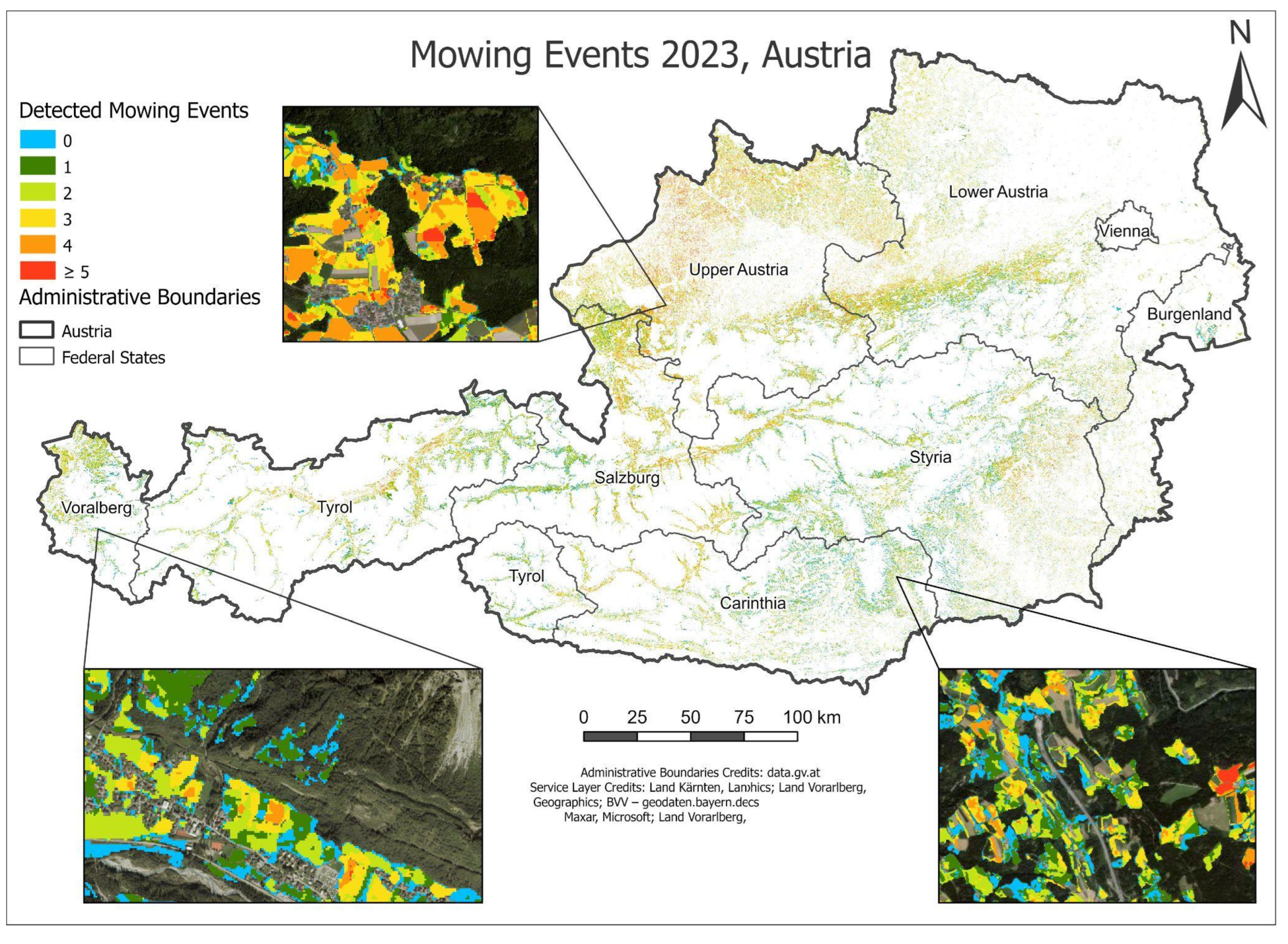
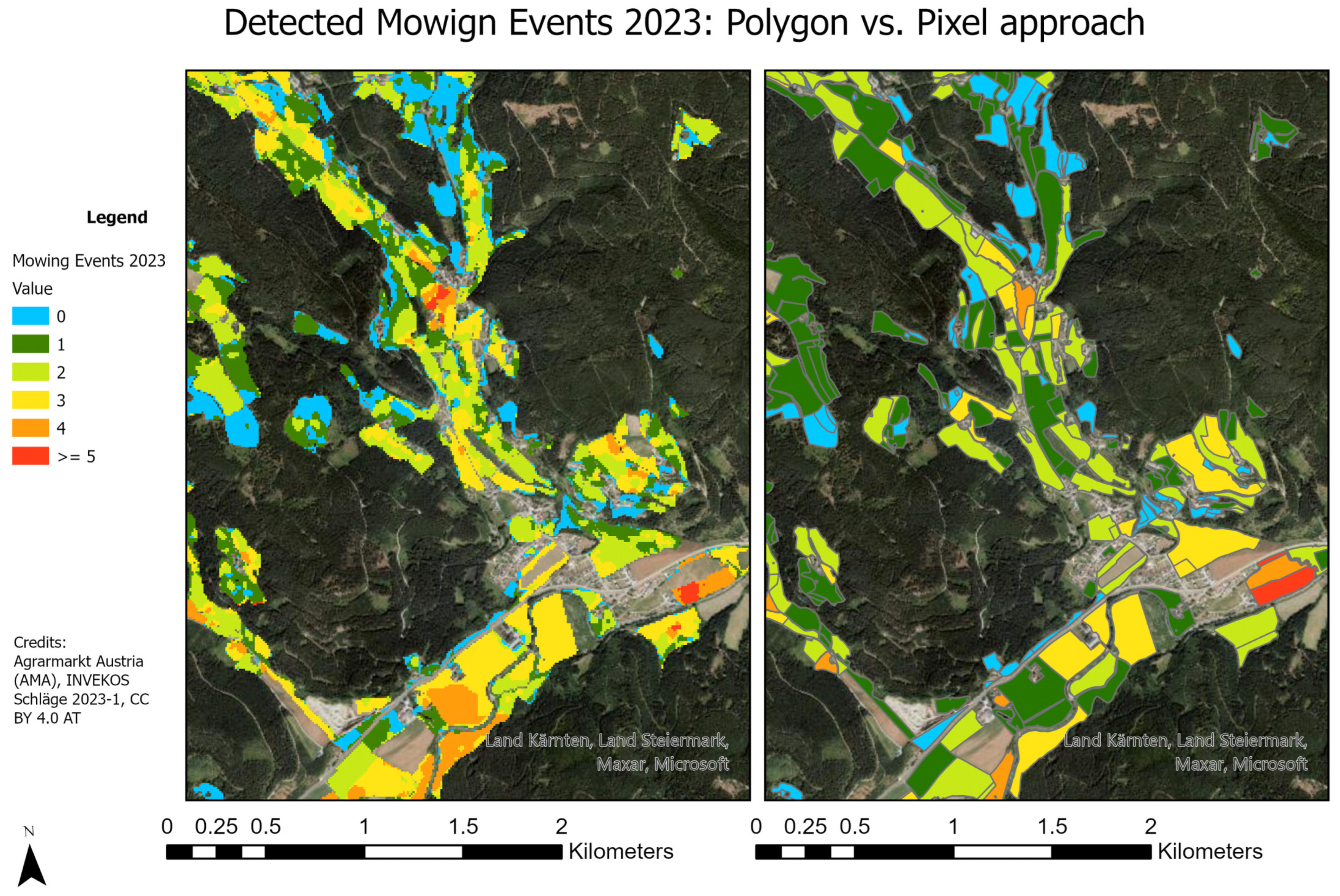
4.1. Mapping Result
4.2. Accuracy Assessment Based on Validation Dataset
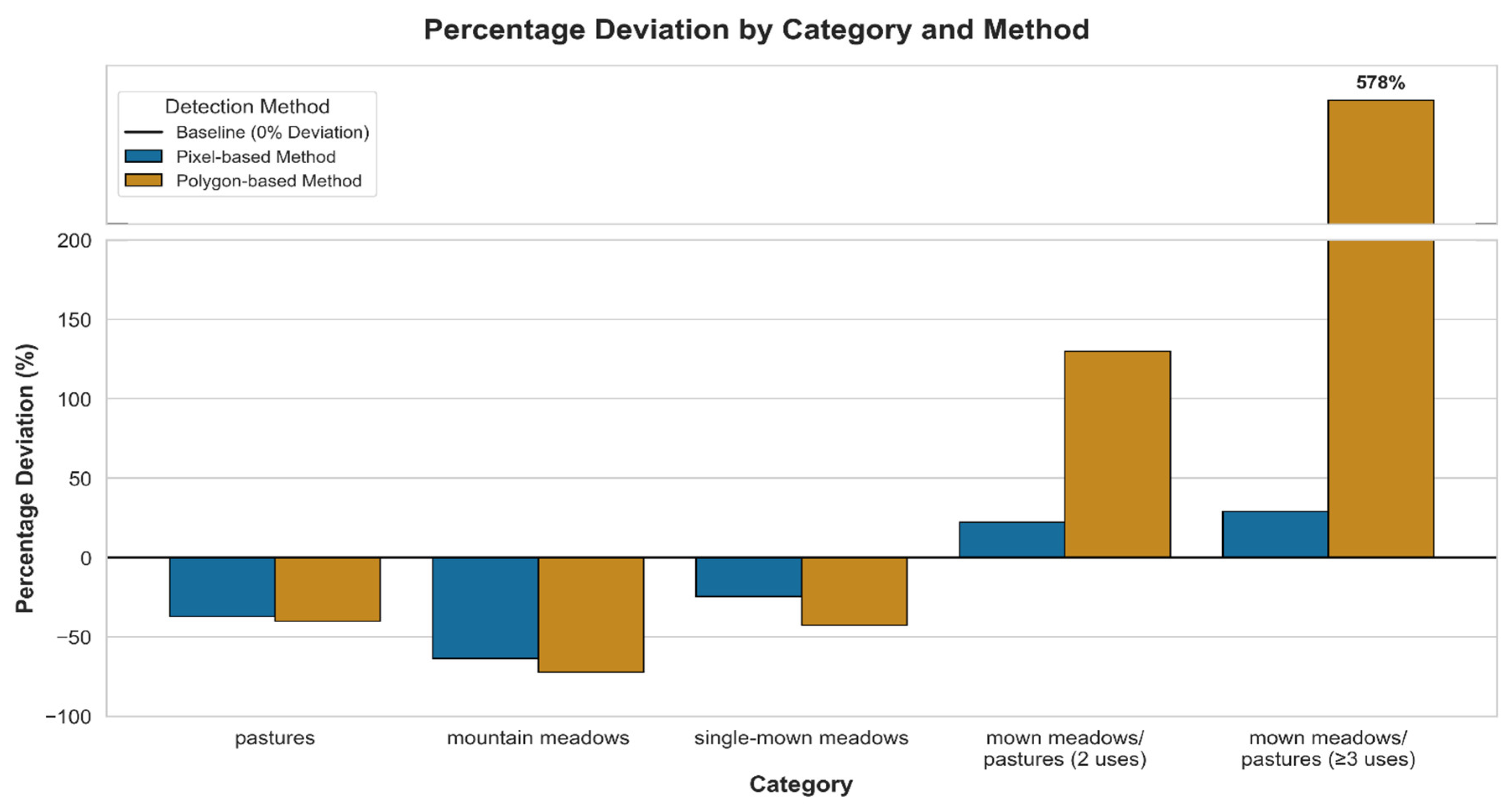
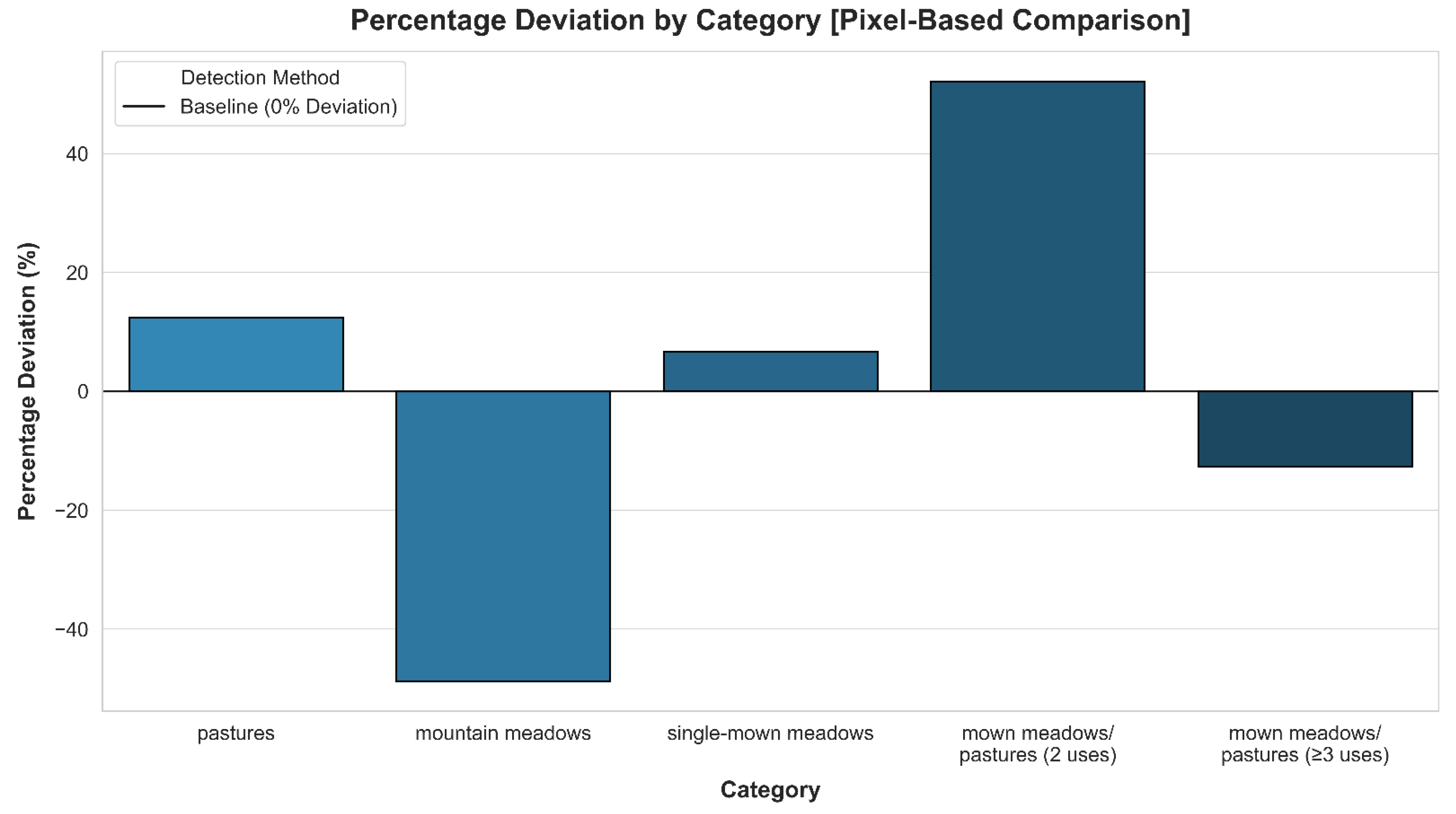
4.3. Plausibility Check in Comparison with IACS Dataset
- (a)
- Pixel-based versus polygon-based for the test site only
- (b)
- Pixel-based comparison with IACS for whole of Austria
5. Discussion
6. Conclusions
Author Contributions
Funding
Data Availability Statement
Acknowledgments
Conflicts of Interest
Appendix A

| Location | Panomax Mowing Events | Panomax Grazing Events | Detected Events | Commission (Only Mowing) | Commission (Incl. Grazing) |
|---|---|---|---|---|---|
| Griffen | 4 | 0 | 4 | 0 | 0 |
| Pyhrn | 5 | 0 | 5 | 0 | 0 |
| Pertisau | 3 | 0 | 5 | 2 | 2 |
| Liebenau | 4 | 0 | 3 | 0 | 0 |
| Nassereith | 2 | 1 | 3 | 1 | 0 |
| Ramsau im Zillertal | 3 | 1 | 4 | 1 | 0 |
| Pertisau | 3 | 0 | 4 | 1 | 0 |
| Scharnitz | 2 | 1 | 4 | 2 | 1 |
| Donnersbachwald | 2 | 1 | 3 | 1 | 1 |
| Altenmarkt 1 | 4 | 0 | 5 | 1 | 0 |
| Altenmarkt 2 | 4 | 1 | 5 | 1 | 1 |
| Mondsee | 5 | 0 | 4 | 0 | 0 |
| Bad Mitterndorf | 4 | 0 | 3 | 0 | 0 |
| Großarl 1 | 4 | 1 | 5 | 1 | 0 |
| Großarl 2 | 4 | 0 | 6 | 2 | 2 |
| Großarl 3 | 4 | 0 | 6 | 2 | 2 |
| Großarl 4 | 3 | 0 | 5 | 2 | 2 |
| Westendorf 1 | 4 | 1 | 4 | 0 | 0 |
| Westendorf 2 | 4 | 0 | 4 | 0 | 0 |
| Westendorf 3 | 3 | 1 | 3 | 0 | 0 |
| Average | 0.9 | 0.6 |
References
- Statistik Austria. Agrarstrukturdatenerhebung 2020; Statistik im Fokus; Statistik Austria: Vienna, Austria, 2022; p. 138. [Google Scholar]
- Griffiths, P.; Nendel, C.; Pickert, J.; Hostert, P. Towards National-Scale Characterization of Grassland Use Intensity from Integrated Sentinel-2 and Landsat Time Series. Remote Sens. Environ. 2020, 238, 111124. [Google Scholar] [CrossRef]
- Halabuk, A.; Mojses, M.; Halabuk, M.; David, S. Towards Detection of Cutting in Hay Meadows by Using of NDVI and EVI Time Series. Remote Sens. 2015, 7, 6107–6132. [Google Scholar] [CrossRef]
- Hartmann, A.; Sudmanns, M.; Augustin, H.; Baraldi, A.; Tiede, D. Estimating the Temporal Heterogeneity of Mowing Events on Grassland for Haymilk-Production Using Sentinel-2 and Greenness-Index. Smart Agric. Technol. 2023, 4, 100157. [Google Scholar] [CrossRef]
- Kolecka, N.; Ginzler, C.; Pazur, R.; Price, B.; Verburg, P.H. Regional Scale Mapping of Grassland Mowing Frequency with Sentinel-2 Time Series. Remote Sens. 2018, 10, 1221. [Google Scholar] [CrossRef]
- Watzig, C.; Schaumberger, A.; Klingler, A.; Dujakovic, A.; Atzberger, C.; Vuolo, F. Grassland Cut Detection Based on Sentinel-2 Time Series to Respond to the Environmental and Technical Challenges of the Austrian Fodder Production for Livestock Feeding. Remote Sens. Environ. 2023, 292, 113577. [Google Scholar] [CrossRef]
- Reinermann, S.; Asam, S.; Kuenzer, C. Remote Sensing of Grassland Production and Management—A Review. Remote Sens. 2020, 12, 1949. [Google Scholar] [CrossRef]
- Buchgraber, K.; Schaumberger, A.; Pötsch, E.M.; Krautzer, B.; Hopkins, A. Grassland Farming in Austria-Status Quo and Future Prospective. Grassl. Sci. Eur. 2011, 16, 95–156. [Google Scholar]
- AgrarMarkt Austria (AMA). Österreichisches Programm zur Förderung Einer Umweltgerechten, Extensiven und den Natürlichen Lebensraum Schützenden Landwirtschaft; AgrarMarkt Austria: Vienna, Austria, 2021; p. 110. [Google Scholar]
- Reinermann, S.; Gessner, U.; Asam, S.; Ullmann, T.; Schucknecht, A.; Kuenzer, C. Detection of Grassland Mowing Events for Germany by Combining Sentinel-1 and Sentinel-2 Time Series. Remote Sens. 2022, 14, 1647. [Google Scholar] [CrossRef]
- Roy, D.P.; Li, J.; Zhang, H.K.; Yan, L.; Huang, H.; Li, Z. Examination of Sentinel-2A Multi-Spectral Instrument (MSI) Reflectance Anisotropy and the Suitability of a General Method to Normalize MSI Reflectance to Nadir BRDF Adjusted Reflectance. Remote Sens. Environ. 2017, 199, 25–38. [Google Scholar] [CrossRef]
- European Space Agency (ESA). S2 MPC: Level-2A Algorithm Theoretical Basis Document; ESA: Paris, France, 2021. [Google Scholar]
- Main-Knorn, M.; Pflug, B.; Louis, J.; Debaecker, V.; Müller-Wilm, U.; Gascon, F. Sen2Cor for Sentinel-2. In Proceedings of the Image and Signal Processing for Remote Sensing XXIII, Warsaw, Poland, 4 October 2017; Bruzzone, L., Ed.; SPIE: San Diego, CA, USA, 2017; Volume 10427, p. 1042704. [Google Scholar] [CrossRef]
- Dechoz, C.; Poulain, V.; Massera, S.; Languille, F.; Greslou, D.; de Lussy, F.; Gaudel, A.; L’Helguen, C.; Picard, C.; Trémas, T. Sentinel 2 Global Reference Image. In Proceedings of the Image and Signal Processing for Remote Sensing XXI, Toulouse, France, 15 October 2015; Bruzzone, L., Ed.; SPIE: San Diego, CA, USA, 2015; Volume 9643, p. 96430A. [Google Scholar] [CrossRef]
- Frantz, D.; Roder, A.; Udelhoven, T.; Schmidt, M. Enhancing the Detectability of Clouds and Their Shadows in Multitemporal Dryland Landsat Imagery: Extending Fmask. Geosci. Remote Sens. Lett. 2015, 12, 1242–1246. [Google Scholar] [CrossRef]
- Minnaert, M. The Reflection of Light in Rippled Surfaces. Physica 1942, 9, 925–935. [Google Scholar] [CrossRef]
- Gallaun, H.; Schardt, M.; Linser, S. Remote Sensing Based Forest Map of Austria and Derived Environmental Indicators. In Proceedings of the ForestSat Conference, Montpellier, France, 5–7 November 2007. [Google Scholar]
- Schwieder, M.; Wesemeyer, M.; Frantz, D.; Pfoch, K.; Erasmi, S.; Pickert, J.; Nendel, C.; Hostert, P. Mapping Grassland Mowing Events across Germany Based on Combined Sentinel-2 and Landsat 8 Time Series. Remote Sens. Environ. 2022, 269, 112795. [Google Scholar] [CrossRef]
- Sudmanns, M.; Tiede, D.; Augustin, H.; Lang, S. Assessing Global Sentinel-2 Coverage Dynamics and Data Availability for Operational Earth Observation (EO) Applications Using the EO-Compass. Int. J. Digit. Earth 2020, 13, 768–784. [Google Scholar] [CrossRef] [PubMed]
- Lobert, F.; Holtgrave, A.-K.; Schwieder, M.; Pause, M.; Vogt, J.; Gocht, A.; Erasmi, S. Mowing Event Detection in Permanent Grasslands: Systematic Evaluation of Input Features from Sentinel-1, Sentinel-2, and Landsat 8 Time Series. Remote Sens. Environ. 2021, 267, 112751. [Google Scholar] [CrossRef]
- Dujakovic, A.; Watzig, C.; Schaumberger, A.; Klingler, A.; Atzberger, C.; Vuolo, F. Enhancing Grassland Cut Detection Using Sentinel-2 Time Series through Integration of Sentinel-1 SAR and Weather Data. Remote Sens. Appl. Soc. Environ. 2025, 37, 101453. [Google Scholar] [CrossRef]
- De Vroey, M.; Radoux, J.; Defourny, P. Grassland Mowing Detection Using Sentinel-1 Time Series: Potential and Limitations. Remote Sens. 2021, 13, 348. [Google Scholar] [CrossRef]
- Tamm, T.; Zalite, K.; Voormansik, K.; Talgre, L. Relating Sentinel-1 Interferometric Coherence to Mowing Events on Grasslands. Remote Sens. 2016, 8, 802. [Google Scholar] [CrossRef]
- Statistik Austria. Bodennutzung 2020; Statistik Austria: Vienna, Austria, 2020. [Google Scholar]
- Schwieder, M.; Lobert, F.; Muhuri, A.; Oppelt, N.; Asam, S.; Reinermann, S.; Morel, J.; Rossi, M.; Weber, D.; Sarvia, F.; et al. Mowing Detection Intercomparison Exercise—MODCiX. In Proceedings of the Earsel Symposium, Bucharest, Romania, 3–6 July 2023. [Google Scholar]


| IACS Category | Definition |
|---|---|
| pasture (Hutweide) | The pasture is a low-yielding, grazed permanent grassland (usually without maintenance cutting) on which mechanical fodder production or maintenance is not possible or is not carried out due to the nature of the soil. These areas must be fully grazed at least once per year. |
| mountain meadow (Bergmähder) | Mountain meadows are extensive mowing areas above the local permanent settlement boundary, whereby these areas must be above the altitude of the home farm and generally not directly adjacent to home farm areas of the same farm. The majority of the area must be above 1200 m.a.s.l. Mountain meadows must be fully mown at least once every two years and the mown material must be removed. |
| single-mown meadow (Mähwiese 1) | Single-mown meadows are areas on which the entire surface is mown once a crop year and the mown material is removed from the area. |
| mown meadow/pasture with two uses (Mähwiese 2) | Mown meadows/pastures with two uses are areas on which full-surface mowing is carried out either twice (including the removal of the mown material) or only once but combined with a full-surface grazing in the same year. A selective maintenance cut does not count. |
| mown meadow/pasture with three or more uses (Mähwiese 3) | Mown meadows/pastures with three or more uses are areas on which full-surface mowing is carried out either three times (including the removal of the mown material) or a combination of one or two mowing events (including the removal of the mown material) with full-surface grazing in the same year to reach at least three full-surface uses. |
| Maximum Allowed Delay | Delay in Cut Detection (Mean Absolute Error-MAE) [Days] | Detection Rate [%] | |||||
|---|---|---|---|---|---|---|---|
| 1 | 2 | 3 | 4 | 5 | All Cuts | ||
| 30 days | 5.3 | 3.3 | 4.1 | 3.9 | 5.7 | 4.30 | 78.67 |
| 15 days | 5.3 | 3.3 | 3.5 | 3.2 | 5.7 | 4.07 | 77.73 |
| 7 days | 3.28 | 2.6 | 2.5 | 2.9 | 3 | 2.84 | 63.98 |
| Month | No. of Reference Mowing Events | Detected Mowing Events [%] | Monthly Mean Cloud Cover over Reference Sites [%] |
|---|---|---|---|
| April | 1 | 0 | 80 |
| May | 40 | 50 | 65 |
| June | 46 | 85 | 59 |
| July | 41 | 73 | 53 |
| August | 34 | 97 | 50 |
| September | 30 | 100 | 30 |
| October | 19 | 68 | 48 |
Disclaimer/Publisher’s Note: The statements, opinions and data contained in all publications are solely those of the individual author(s) and contributor(s) and not of MDPI and/or the editor(s). MDPI and/or the editor(s) disclaim responsibility for any injury to people or property resulting from any ideas, methods, instructions or products referred to in the content. |
© 2025 by the authors. Licensee MDPI, Basel, Switzerland. This article is an open access article distributed under the terms and conditions of the Creative Commons Attribution (CC BY) license (https://creativecommons.org/licenses/by/4.0/).
Share and Cite
Miletich, P.; Kirchmair, M.; Deutscher, J.G.; Schippl, A.; Hirschmugl, M. Open and Free Sentinel-2 Mowing Event Data for Austria. Remote Sens. 2025, 17, 1769. https://doi.org/10.3390/rs17101769
Miletich P, Kirchmair M, Deutscher JG, Schippl A, Hirschmugl M. Open and Free Sentinel-2 Mowing Event Data for Austria. Remote Sensing. 2025; 17(10):1769. https://doi.org/10.3390/rs17101769
Chicago/Turabian StyleMiletich, Petra, Marco Kirchmair, Janik Gregory Deutscher, Alexander Schippl, and Manuela Hirschmugl. 2025. "Open and Free Sentinel-2 Mowing Event Data for Austria" Remote Sensing 17, no. 10: 1769. https://doi.org/10.3390/rs17101769
APA StyleMiletich, P., Kirchmair, M., Deutscher, J. G., Schippl, A., & Hirschmugl, M. (2025). Open and Free Sentinel-2 Mowing Event Data for Austria. Remote Sensing, 17(10), 1769. https://doi.org/10.3390/rs17101769