Machine Learning-Based Estimation of foF2 and MUF(3000)F2 Using GNSS Ionospheric TEC Observations

Abstract

This study developed machine learning models using different algorithms, including support vector machine (SVM), random forest (RF), and backpropagation neural network (BPNN), to estimate the critical frequency of the F2 layer (foF2) and the maximum usable frequency of the F2 layer for a 3000 km circuit (MUF(3000)F2) based on the total electron content (TEC) observed by global navigation satellite system (GNSS) receivers. The ionospheric dataset used comprised TEC, foF2, and MUF(3000)F2 measurements from 11 stations in China during a solar activity period (2008–2020). The results indicate that all three machine learning models performed better than the IRI-2020 model, with varying levels of accuracy. For foF2 (MUF(3000)F2) estimation, the root mean square error (RMSE) values at Kunming and Xi’an stations were reduced by approximately 38% (26%) and 18% (11%), respectively, compared to IRI-2020. During geomagnetic disturbances, all three models were able to reproduce the variations in both foF2 and MUF(3000)F2 parameters. Nevertheless, the RF model showed significantly better performance in foF2 estimation compared to the SVM and BPNN models.

1. Introduction

The ionosphere is located at an altitude of 60 km to 1000 km above the ground and is produced by ionization of the Earth’s atmosphere, due to solar radiation (mainly extreme ultraviolet (EUV) and X-rays). The state of the ionosphere is complex and shows variations in the influences from solar activity, geomagnetic activity, geographical location, season and local time [1]. In order to study the morphological characteristics of the ionosphere, a variety of parameters have been proposed to describe the characteristics of the ionosphere, including the critical frequency of the F2 layer (foF2), the maximum usable frequency of the F2 layer for a 3000 km circuit (MUF(3000)F2), and the ionospheric total electron content (TEC). The foF2 gives the highest frequency when the radio waves emitted vertically from the ground can be reflected back to ground by the F2 layer. Maximum usable frequency (MUF) refers to the highest frequency at which radio waves can be received from a specific path when reflected by the ionosphere, and MUF(3000)F2 represents the maximum usable frequency when the radio waves can be reflected and received over a horizontal distance of 3000 km. These parameters can not only help high frequency (HF) radio users to determine the frequency for communication, but also provide useful information about the background ionosphere, which can be used for further ionospheric related studies.

According to [2], the foF2 is closely related to MUF(3000)F2, and the relationship between them is shown in Equation (1) [2].

$$\mathrm{MUF}\left(3000\right)\mathrm{F}2=\mathrm{foF}2 \times \mathrm{M}\left(3000\right)\mathrm{F}2$$

(1)

In Equation (1), MUF(3000)F2 and foF2 units are both MHz, and M(3000)F2 is the propagation factor, which is dimensionless. The detection of foF2 and MUF(3000)F2 mainly depends on the ionosondes. The foF2 can be read from the ionograms obtained by the ionosondes, while the MUF(3000)F2 can be calculated using Equation (1) after reading foF2 and M(3000)F2 from the ionograms. However, ionosondes are relatively expensive and distributed quite sparsely from the perspective of global coverage, resulting in costly foF2 and MUF(3000)F2 data acquisition. Therefore, it is necessary to find an alternative method to acquire foF2 and MUF(3000)F2 information at locations with less ionosonde coverage.

Earlier attempts have been made to estimate the foF2 value using TEC values provided by the ground-based networks of global navigation satellite system (GNSS) receivers. Spalla and Cairolo described the relationship between foF2 and TEC as Equation (2) [3] as follows:

$${\left(\mathrm{foF}2\right)}^2=3.51\mathrm{TEC}$$

(2)

In Equation (2), the unit of foF2 is MHz, the unit of TEC is TECU, and 1 TECU = 10¹⁶ electrons/m². However, the equation can only give a rough estimate of foF2, as the correlation between foF2 and TEC is also affected by time, geographical location, as well as the solar flux and geomagnetic activities. To obtain the estimation of foF2 instantaneous values, Vivian Otugo et al. [4] constructed a model using neural networks to estimate the foF2, which used TEC, day of year (DOY), local time (LT), sunspot number (SSN), and Dst index as inputs, and the root mean square error (RMSE) of the model is less than 1 MHz. Though their study demonstrated the feasibility of using TEC to estimate foF2 through a neural network, it did not evaluate the performance of the neural network model in detail to analyze the accuracy of the model in different cases, such as under quiet or disturbed ionospheric conditions. To the knowledge of the authors, no study on the relationship between MUF(3000)F2 and TEC correlation has been conducted to explore the possibility of estimating MUF(3000)F2 by TEC observation.

Machine learning can find laws of big data, establish appropriate models based on massive data, and fit complex nonlinear functions. It is often used for parameter prediction or estimation. With the improvement in computer performance and the increasing amount of data, machine learning has made great progress and is widely used in business and scientific fields. Of these, the most widely used machine learning models are RF, SVM and artificial neural networks (ANN). In the field of ionosphere, machine learning has been widely used to model ionospheric parameters with good results. Hernandez-Pajares et al., 1997, used GPS data to establish a global-scale electron content model through neural networks [5]. Poole and Mckinnell (2000) used neural networks to establish a 1 h ahead ionospheric foF2 prediction model [6]. Oyeyemi (2005) used neural networks to establish a global empirical model of foF2 with better accuracy than the international reference ionospheric model (IRI) [7,8]. Nakamura et al., 2007, used neural networks to establish a 24 h ahead foF2 prediction model that captures partially the foF2 variability during ionospheric storms [9]. Leandro and Santos (2007) established a regional TEC model by neural network estimation using Brazilian GPS data [10]. Habarulema et al., 2007 used neural networks to predict TEC over South Africa [11]. Habarulema and McKinnell (2012) studied the performance of TEC estimation of five neural network backpropagation training algorithms built into the Stuttgart Neural Network Simulator (SNNS) [12]. Gowtam and Ram (2017) established neural network prediction models for NmF2 and hmF2 using FORMOSAT-3/COSMIC radio occultation observations [13]. Song et al., 2018 used a genetic algorithm-optimized neural network to establish a TEC prediction model for the China region [14]. Fan et al., 2019 used a particle swarm algorithm (IPSO)-optimized Elman neural network to establish a foF2 prediction model 1 h ahead [15]. Zhao (2019) used a genetic algorithm (GA)-optimized BPNN to predict foF2 perturbations 1–24 h ahead [16]. Xia et al., 2021 used a graphics processing unit (GPU) to accelerate SVM-model training to establish a TEC prediction model for the China region [17]. With the development of machine learning, deep learning algorithms are also used for modeling ionospheric parameters. Sun et al., 2017 predicted TEC of Beijing using a long short-term memory network (LSTM) [18]. Kaselimi et al., 2020 made a comparison of the performance between an LSTM and a traditional stochastic model of TEC [19]. Li et al., 2021, used LSTM to establish a model for foF2 prediction, and the LSTM model made better predictions compared to the BPNN model [20]. However, fewer studies have focused on comparing the performance of different algorithms used to forecast ionospheric parameters by modeling ionospheric parameters using machine learning.

The purpose of this paper is to develop a model for estimating foF2 and MUF(3000)F2 using TEC, based on machine learning techniques. Due to the scarcity of ionosonde stations, foF2 and MUF(3000)F2 data are difficult and expensive to obtain, while GNSS receiver stations are dense and TEC data are easy and inexpensive to obtain; incorporating this model into GNSS receivers can help people obtain TEC, foF2 and MUF(3000)F2 parameters in real-time through GNSS receivers only. This is important in areas where ionosondes are sparse or lacking. In addition, the method can take advantage of the good integrity of TEC data to supplement the missing data of the ionosonde to investigate the performance of different types of machine learning algorithms for estimating foF2 and MUF(3000)F2. Therefore, the algorithms RF, SVM and BPNN, which are the most widely used in neural networks, were selected for modeling, and the evaluation results may guide people to choose the appropriate machine learning algorithm to estimate foF2 and MUF(3000)F2.

In this paper, Section 2 describes the principles of three machine learning models, RF, SVM, and BPNN, along with the input and output parameters of models and the datasets used. The estimation results of foF2 and MUF(3000)F2 are shown and analyzed in Section 3. Section 4 discusses the findings. Finally, Section 5 summarizes the entire article.

2. Materials and Methods

2.1. Description of Machine Learning Algorithms

In this paper, the RF algorithm based on the decision tree, SVM algorithm and BPNN algorithm which are most widely used in neural networks, are selected for modeling. In the following, we briefly introduce the principles of RF, SVM and BPNN, three machine learning algorithms.

2.1.1. RF Algorithm

The RF algorithm is an ensemble learning algorithm based on decision trees, which uses bootstrap aggregating to combine multiple decision trees into a forest to predict the results. Bootstrap aggregation, also known as bagging, is an algorithm that trains a weak learner by reselecting multiple new datasets on the original dataset through sampling with replacement [21]. This method divides the original dataset into n new training sets, constructs a weak learner on each new training set, and integrates the results of these n weak learners using majority voting (for classification problems) or averaging the output of each weak learner (for regression problems) to obtain the result. The weak learners in the RF are decision trees, which can be classified into classification trees and regression trees, depending on the type of dependent variable data, and the type of decision tree determines whether the RF is used for classification or regression. RF is simple to implement, has high accuracy and strong generalization ability. The introduction of randomness makes it less likely to fall into overfitting, and has a certain ability of anti-noise. In addition, because each decision tree can be generated independently and simultaneously, the algorithm is faster and easier to parallelize than other machine learning algorithms. Figure 1 shows the flowchart of the RF algorithm. The algorithmic workflow of the RF method proceeds as follows:

Step 1: Bootstrap sampling is performed on the original dataset with replacements to generate m distinct training subsets.

Step 2: For each training subset, a random selection of K features is made (K being smaller than the total number of features in the original dataset).

Step 3: Multiple decision trees (n trees) are iteratively constructed based on these K features.

Step 4: Each decision tree is employed to generate predictions, with all prediction outcomes being recorded.

Step 5: The predictions from all decision trees are aggregated as follows:

(1) For classification tasks, a majority voting scheme is implemented, wherein the class receiving the highest number of votes is selected as the final output.

(2) For regression tasks, the final prediction is derived by computing the average of all individual tree predictions.

This ensemble approach enhances model robustness by combining multiple weak learners while mitigating overfitting through feature and data randomization.

2.1.2. SVM Algorithm

SVM is built on the Vapnik–Chervonenkis dimension theory and the principle of structural risk minimization [22]. It seeks the best compromise between the complexity of the model (the accuracy of learning for a given training sample) and the learning ability (the ability to identify arbitrary samples without errors) based on limited sample information, with the aim of obtaining the best generalization ability. Unlike other machine learning algorithms, SVM is supported by strict mathematical theory and does not rely on empirical or prior knowledge, and has good function approximation capability and robustness. SVM is essentially a solution to a quadratic minimization problem (convex optimization problem) under constraints. Theoretically, the local optimal solution of a convex optimization problem must be the global optimal solution, while other machine learning algorithms such as neural networks can generally only obtain the local optimal solution. SVM is widely used for solving classification or regression problems with its own advantages. The support vector regression problem can be expressed as follows:

$$\min {\displaystyle \frac{1}{2}}{‖\mathrm{w}‖}^2 +\mathrm{C}\sum _{\mathrm{i}=1}^{\mathrm{m}}{\mathrm{l}}_{\mathsf{ϵ}}\left(\mathrm{f}\left({\mathrm{x}}_{\mathrm{i}}\right)-{\mathrm{y}}_{\mathrm{i}}\right)$$

(3)

where C denotes the regularization constant, and ${\mathrm{l}}_{\mathsf{ϵ}}$ represents the ϵ-insensitive loss function.

By introducing slack variables ${\mathsf{\xi }}_{\mathrm{i}}$ and ${\widehat{\mathsf{\xi }}}_{\mathrm{i}}$, Equation (3) can be rewritten as the following:

$$\min {\displaystyle \frac{1}{2}}{‖\mathrm{w}‖}^2+\mathrm{C}\sum _{\mathrm{i}=1}^{\mathrm{m}}{\mathrm{l}}_{\mathsf{ϵ}}\left({\mathsf{\xi }}_{\mathrm{i}}+{\widehat{\mathsf{\xi }}}_{\mathrm{i}}\right)$$

(4)

$$\mathrm{s}.\mathrm{t}. \mathrm{f}\left({\mathrm{x}}_{\mathrm{i}}\right)-{\mathrm{y}}_{\mathrm{i}}\le \mathsf{ϵ}+ {\mathsf{\xi }}_{\mathrm{i}}$$

(5)

$$\begin{gathered} {\mathrm{y}}_{\mathrm{i}}-\mathrm{f}\left({\mathrm{x}}_{\mathrm{i}}\right)\le \mathsf{ϵ}+ {\widehat{\mathsf{\xi }}}_{\mathrm{i}} \\ {\mathsf{\xi }}_{\mathrm{i}} \ge 0, {\widehat{\mathsf{\xi }}}_{\mathrm{i}} \ge 0, \mathrm{i}=1,2,\dots ,\mathrm{m} \end{gathered}$$

(6)

Introducing Lagrange multipliers ${\mathsf{\mu }}_{\mathrm{i}} \ge 0$, ${\widehat{\mathsf{\mu }}}_{\mathrm{i}} \ge 0$, ${\mathsf{\alpha }}_{\mathrm{i} }\ge 0$, ${\widehat{\mathsf{\alpha }}}_{\mathrm{i}} \ge 0$, we construct the Lagrangian equation via the method of Lagrange multipliers. Subsequently, based on duality theory, the minimization problem is transformed into its dual problem (a maximization problem). Solving this yields the following regression function:

$$\mathrm{f}\left(\mathrm{x}\right)=\sum _{\mathrm{i}=1}^{\mathrm{m}}\left({\widehat{\mathsf{\alpha }}}_{\mathrm{i}}-{\mathsf{\alpha }}_{\mathrm{i}}\right)\mathsf{\kappa }\left(\mathrm{x},{\mathrm{x}}_{\mathrm{i}}\right)+\mathrm{b}$$

(7)

where $\mathsf{\kappa }\left({\mathrm{x}}_{\mathrm{i}},{\mathrm{x}}_{\mathrm{j}}\right)=\mathsf{\varphi }{\left({\mathrm{x}}_{\mathrm{i}}\right)}^{\mathrm{T}}\mathsf{\varphi }\left({\mathrm{x}}_{\mathrm{j}}\right)$ denotes the kernel function. For nonlinear regression estimation, the fundamental concept involves mapping samples from the original space to a higher-dimensional feature space through a predetermined nonlinear mapping $\mathsf{\varphi }\left(\mathrm{x}\right)$. Linear regression is then performed in this high-dimensional feature space, thereby achieving the effect of nonlinear regression approximation in the original space.

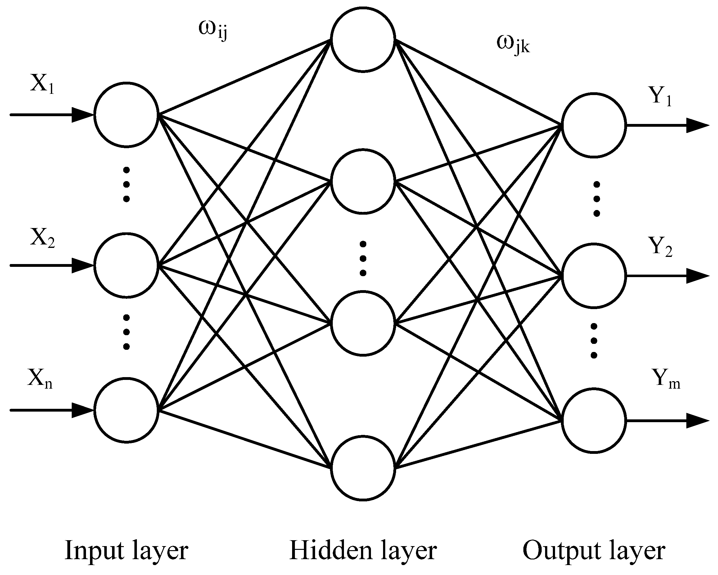
2.1.3. BPNN Algorithm

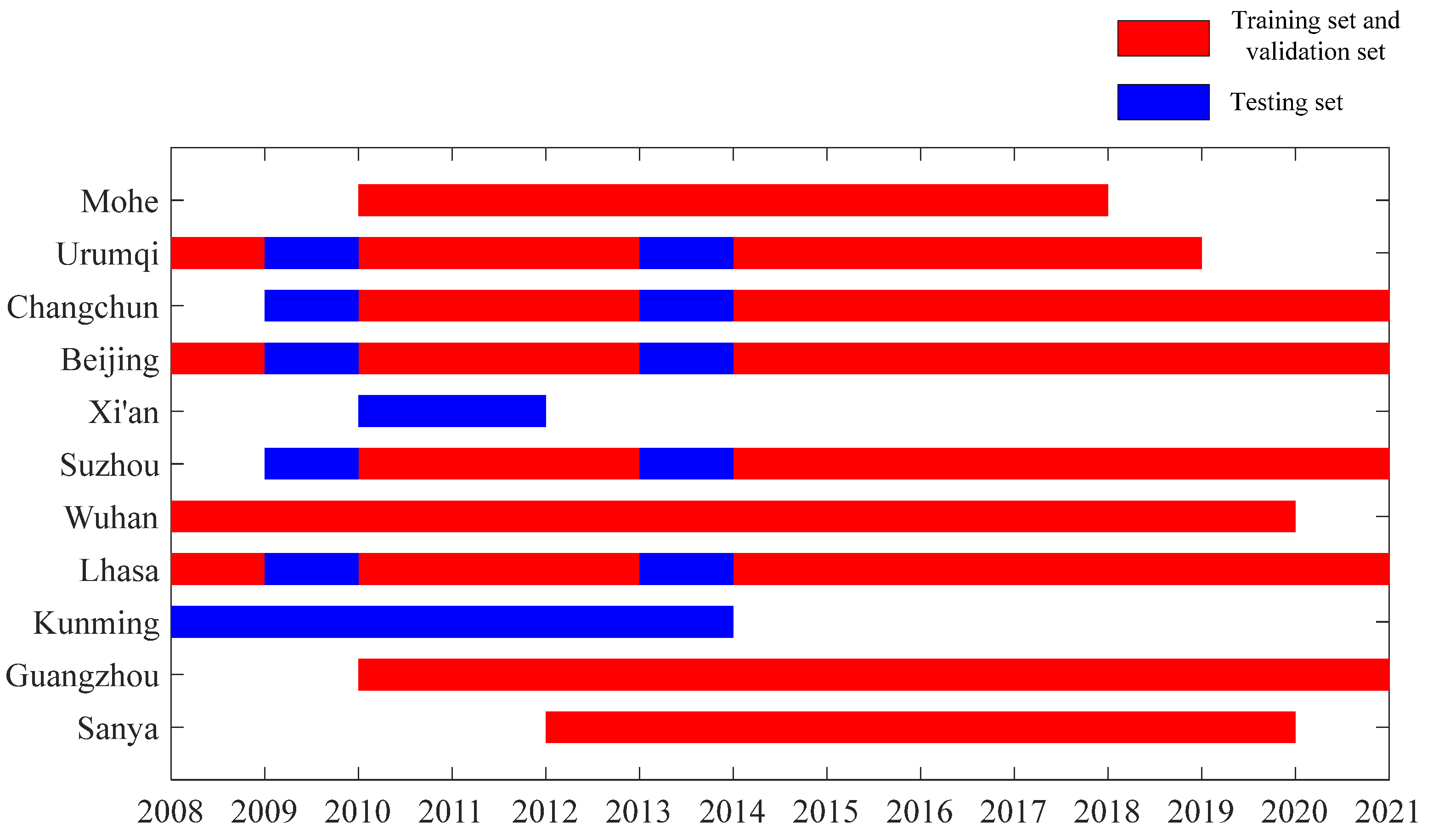
The back propagation algorithm is the most successful neural network algorithm so far. Most of the neural networks used in practical applications are trained by the back propagation algorithm [23]. The BPNN generally refers to the multi-layer feedforward neural network trained by the back propagation algorithm. The main characteristics of the network are signal forward transmission and error back propagation. In the forward transmission, the input signal is processed layer by layer from the input layer through the hidden layer until the output layer. The neuron state in each layer only affects the neuron state in the next layer. If the output layer cannot obtain the desired output, it will turn to back propagation and adjust the network weight and threshold according to the prediction error, so that the predicted output of BPNN is constantly approaching the desired output. BPNN is widely used to solve classification and regression problems due to its powerful nonlinear mapping ability, generalization and fault tolerance. The topological structure of BPNN is shown in Figure 2.

In Figure 2, X₁, X₂, …, Xn are the input values of BPNN, Y₁, Y₂, …, Ym are the output values of BPNN, ω_ij and ω_jk are the weights of BPNN, respectively, and BPNN expresses the function mapping relationship from n independent variables to m dependent variables. The algorithmic workflow of the BPNN is as follows:

Step 1: Network Initialization.

Assume the network has n input layer nodes, l hidden layer node, and m output layer nodes. Let ω_ij denote the connection weights between the input layer and hidden layer neurons, and ω_jk represent the connection weights between the hidden layer and output layer neurons. The hidden layer threshold is denoted as a, and the output layer threshold as b. Given the learning rate η and the neuronal activation function g(x), this study employs the Sigmoid function as the activation function, whose mathematical expression is shown in Equation (8).

$$\mathrm{g}\left(\mathrm{x}\right)={\displaystyle \frac{1}{1+{\mathrm{e}}^{-\mathrm{x}}}}$$

(8)

Step 2: Hidden Layer Output Calculation.

Given the input vector X, the connection weights ω_ij between the input layer and hidden layer, and the hidden layer threshold a, the hidden layer output H can be expressed by Equation (9).

$${\mathrm{H}}_{\mathrm{j}}=\mathrm{g}\left(\sum _{\mathrm{i}=1}^{\mathrm{n}}{\mathsf{\omega }}_{\mathrm{ij}}{\mathrm{x}}_{\mathrm{i}}+{\mathrm{a}}_{\mathrm{j}}\right)$$

(9)

Step 3: Output Layer Computation.

Based on the hidden layer output H, connection weights ω_jk, and threshold b, the output O of the BPNN’s output layer is given by Equation (10).

$${\mathrm{O}}_{\mathrm{k}}=\sum _{\mathrm{j}=1}^{\mathrm{l}}{\mathrm{H}}_{\mathrm{j}}{\mathsf{\omega }}_{\mathrm{jk}}{-\mathrm{b}}_{\mathrm{k}}$$

(10)

Step 4: Error Calculation.

Given the neural network output O and the desired output Y, the prediction error e is computed as shown in Equation (11).

$${\mathrm{e}}_{\mathrm{k}}={\mathrm{Y}}_{\mathrm{k}}-{\mathrm{O}}_{\mathrm{k}}$$

(11)

Step 5: Weight Update.

Based on the network’s prediction error e, the connection weights ω_ij and ω_jk are updated according to Equations (12) and (13), respectively.

$${\mathsf{\omega }}_{\mathrm{ij}}={\mathsf{\omega }}_{\mathrm{ij}}+\mathsf{\eta }{\mathrm{H}}_{\mathrm{j}}\left(1 {- \mathrm{H}}_{\mathrm{j}}\right)\mathrm{x}\left(\mathrm{i}\right)\sum _{\mathrm{k}=1}^{\mathrm{m}}{\mathsf{\omega }}_{\mathrm{jk}}{\mathrm{e}}_{\mathrm{k}}$$

(12)

$${\mathsf{\omega }}_{\mathrm{jk}}={\mathsf{\omega }}_{\mathrm{jk}}+\mathsf{\eta }{\mathrm{H}}_{\mathrm{j}}{\mathrm{e}}_{\mathrm{k}}$$

(13)

Step 6: Threshold Update.

The network node thresholds a and b are updated based on the prediction error e, following Equations (14) and (15), respectively.

$${\mathrm{a}}_{\mathrm{j}}={\mathrm{a}}_{\mathrm{j}}+\mathsf{\eta }{\mathrm{H}}_{\mathrm{j}}\left(1 -{ \mathrm{H}}_{\mathrm{j}}\right)\sum _{\mathrm{k}=1}^{\mathrm{m}}{\mathsf{\omega }}_{\mathrm{jk}}{\mathrm{e}}_{\mathrm{k}}$$

(14)

$${\mathrm{b}}_{\mathrm{k}}={\mathrm{b}}_{\mathrm{k}}+{\mathrm{e}}_{\mathrm{k}}$$

(15)

After the above steps are completed, determine whether the algorithm has converged. If it has not converged, return to step 2 and loop until the algorithm converges or the number of loops reaches the set maximum value to obtain the optimal neural network model.

2.2. Datasets

In this work, the foF2 and MUF(3000)F2 observations of the ionosondes are obtained from the China Research Institute of Radiowave Propagation and National Earth System Science Data Center, National Science and Technology Infrastructure of China (http://www.geodata.cn (accessed on 15 October 2024)). The temporal resolution of the data is 1 h, and the data are manually determined. GNSS observation files were obtained from Wuhan University IGS Data Center (http://www.igs.gnsswhu.cn (accessed on 19 October 2024)) and National Earth System Science Data Center, National Science and Technology Infrastructure of China. We use the GPS-TEC analysis application developed by Gopi Seemala (http://seemala.blogspot.com/ (accessed on 21 October 2024)) to process the GNSS observational data to obtain TEC values, with a temporal resolution of 30 s for the data. The temporal resolution of the dataset is the same as the foF2 and MUF(3000)F2 data temporal resolution.

To estimate foF2 and MUF(3000)F2 by TEC, the selection of stations requires GNSS receiver stations to be as close as possible to the corresponding ionosonde stations so that we can obtain the minimum error when building the machine learning model. We select stations based on the criterion that the great circle distance between GNSS receiver stations and their corresponding ionosonde stations is less than 1.5° [4]. Then, a total of 11 GNSS receiver stations and 11 corresponding ionosonde stations are selected.

The distribution of the ionosonde stations and their corresponding GNSS receiver stations used in this work is shown in Figure 3, and the detailed information of the stations is shown in

Table 1. Detailed information of ionosonde stations and corresponding GNSS receiver stations.

Site Name	Ionosonde Station		GNSS Receiver Station		Time Span
	Latitude (°N)	Longitude (°E)	Latitude (°N)	Longitude (°E)
Mohe	53.49	122.34	53.49	122.34	2011–2017
Urumqi	43.75	87.64	43.80	87.60	2008–2018
Changchun	43.84	125.28	43.79	125.44	2009–2020
Beijing	40.11	116.28	39.61	115.89	2008–2020
Xi’an	34.13	108.83	34.37	109.22	2010–2011
Suzhou	31.34	120.41	31.10	121.20	2009–2020
Wuhan	30.60	114.40	30.53	114.36	2008–2019
Lhasa	29.64	91.18	29.66	91.10	2008–2020
Kunming	25.64	103.72	25.03	102.80	2008–2013
Guangzhou	23.14	113.36	22.37	113.93	2010–2020
Sanya	18.35	109.62	18.35	109.62	2012–2019

. Most ionosonde stations and corresponding GNSS receiver stations are located in the same city, while a few ionosonde stations and corresponding GNSS receiver stations are located in neighboring cities, such as Suzhou ionosonde station and Shanghai GNSS receiver station, Guangzhou ionosonde station and Hong Kong GNSS receiver station. For the convenience of naming, we use the name of the city where the ionosonde station is located to name the stations in Figure 3. Owing to obstructions and intermittent interference during observational acquisition, the raw data suffer from discontinuities. Such data gaps are particularly prominent in foF2 records during periods of ionospheric disturbance, when parameter variations exhibit significant deviations from quiet-time conditions. Since conventional data imputation techniques cannot reliably preserve the physical consistency of reconstructed values during disturbed periods, we implemented strict quality control by systematically excluding all outliers and missing data points during training set compilation to maintain model fidelity.

The dataset used in this study cover years longer than one solar cycle (2008–2020). Detailed information of ionosonde stations and corresponding GNSS receiver stations is listed in Table 1. All data of Xi’an station and Kunming station and the data of the other five stations (Urumqi, Changchun, Beijing, Suzhou and Lhasa) from 2013 (high solar activity year) and 2009 (low solar activity year) are used as the test set to evaluate the performance of the machine learning models, and the other data are used to train the model. The training data are divided into the training set and the validation set. The validation set consists of 20% of the data randomly selected from the training data, which is used to test the model configuration and assist in building the model, and the remaining data are used as the training set. Figure 4 shows the time span of the training data and the test data. The training data contains the training set and the validation set.

2.3. Input and Output Parameters

Considering the effects of solar and geomagnetic activity, time and geographic location on foF2 and MUF3000F2, the input parameters of the machine learning model include three components in addition to TEC: solar activity, geomagnetic activity, and spatiotemporal information containing day of year (DOY), local time, and geographic latitude and longitude [24,25]. The specific input parameters are selected as follows.

2.3.1. Solar Activity Parameters

It is well known that solar EUV radiation is an important factor affecting the ionospheric variation, but the observed data of solar EUV radiation spectra are relatively scarce, and solar activity indices are needed to measure the strength of solar EUV radiation. The commonly used solar activity indices are sunspot number (SSN), 10.7 cm radio flux (F10.7), He 1083 index, Mg II, etc. The parameters of sunspot number and F10.7 have better continuity than the others, which are both suitable for the training of machine learning models. However, studies later found that the correlation between either of these parameters and EUV radiation is not ideal on a short time scale, and then an improved solar activity index F10.7P was proposed. The formula is shown in Equation (16), where F10.7A is the 81-day sliding average of F10.7. Compared with sunspot number and F10.7, F10.7P has a better linear correlation with EUV radiation and can better characterize the solar EUV radiation level. In this paper, the parameter of F10.7P is chosen to characterize the intensity of solar activity [26].

$$\mathrm{F}10.7\mathrm{P}={\displaystyle \frac{\mathrm{F}10.7+\mathrm{F}10.7\mathrm{A}}{2}}$$

(16)

2.3.2. Geomagnetic Activity Parameters

Geomagnetic activity also has important effects on ionosphere,; for example, magnetic storms: the ionosphere is usually violently disturbed by magnetic storms. Therefore, geomagnetic activity parameters should be taken as input parameters for forecasting the ionosphere. There are many parameters to characterize geomagnetic activity, such as Kp, ap, Dst, AE, etc. Previous studies found that the Dst index has a strong correlation with foF2 at low latitudes (Wang et al., 2008) [27], and Kp has a strong correlation with foF2 at mid-latitudes (Kutiev and Muhtarov, 2001) [28]. Therefore, this paper uses Dst and Kp indices to characterize the effect of geomagnetic activity on the ionosphere.

2.3.3. Parameters of Spatiotemporal Information

The parameters of spatiotemporal information include DOY, LT and geographical latitude and longitude. To ensure the continuity of values on the midnight boundary (24:00 h LT and 01:00 h LT) and the year-end boundary (31 December and 1 January of the following year), we use Equations (17)–(20) to obtain the values of day of year and local time [29,30,31].

$$\mathrm{DNs}=\sin \left({\displaystyle \frac{2\mathsf{\pi } \times \mathrm{DN}}{365.25}}\right)$$

(17)

$$\mathrm{DNc}=\cos \left({\displaystyle \frac{2\mathsf{\pi } \times \mathrm{DN}}{365.25}}\right)$$

(18)

$$\mathrm{LTs}=\sin \left({\displaystyle \frac{2\mathsf{\pi } \times \mathrm{LT}}{24}}\right)$$

(19)

$$\mathrm{LTc}=\cos \left({\displaystyle \frac{2\mathsf{\pi } \times \mathrm{LT}}{24}}\right)$$

(20)

This work aims to estimate foF2 and MUF(3000)F2, so the output parameters of the machine learning model are foF2 and MUF(3000)F2. The input and output of the machine learning model are shown in Figure 5.

2.4. Model Setting

To obtain the optimal parameter combination for the machine learning model, parameter tuning is required. In this study, the optimal parameter combinations for estimating foF2 and MUF(3000)F2 may differ. We employed a systematic grid search approach to exhaustively evaluate predefined parameter combinations in order to identify the optimal parameter sets for estimating both foF2 and MUF(3000)F2. The root mean square error (RMSE) minimization criterion served as the objective metric for determining the optimal parameter configurations. For estimating foF2, the optimal number of decision trees for the RF model is set to 300 and the number of leaves is 5. The kernel function of the SVM model is set as a Gaussian kernel with kernel scale $\sqrt{\mathrm{p}}$, where p is the number of input variables, p = 8; The number of nodes in the input layer of BPNN is 10, the number of nodes in the hidden layer is 14 and the number of nodes in the output layer is 1. For estimating MUF(3000)F2, the optimal number of decision trees and leaves of the RF model is 350 and 5, respectively. The kernel function setting of the SVM model is the same as that of foF2 estimation. The number of nodes in the input layer of BPNN is 10, the number of nodes in the hidden layer is 17 and the number of nodes in the output layer is 1.

We train the machine learning model in this paper with a computer with Intel (R) Xeon(R) Gold 5220 CPU and NVIDIA GeForce RTX 2080 Ti GPU.

Table 2. Size and training speed of the three machine learning models.

Type	Size	Time to Spend
SVM	52.5 MB	about 25.8 h
RF	1.25 GB	about 0.58 h
BPNN	11.4 MB	about 1.2 h

lists the model size and training speed of the three machine learning models. It can be seen from Table 2 that the size of the SVM model is small, but the training speed is slow. The RF model size is large, but the training speed is fast. The BPNN model size is small, and the training speed is much faster than SVM.

2.5. Error Analysis Method

To evaluate the performance of the different machine learning models, we calculate root mean square error (RMSE), mean absolute percentage error (MAPE), and correlation coefficient (ρ). Of these, RMSE and MAPE can reflect the accuracy of the models, while ρ reflects the correlation between the model results and the observation results. RMSE, MAPE, and ρ are, respectively, calculated by the following Equations (21)–(23).

$$\mathrm{RMSE}=\sqrt{{\displaystyle \frac{1}{\mathrm{m}}}\sum _{\mathrm{i}=1}^{\mathrm{m}}{\left({\mathrm{y}}_{\mathrm{obs},\mathrm{i}} - {\mathrm{y}}_{\mathrm{fore},\mathrm{i}}\right)}^2}$$

(21)

$$\mathrm{MAPE}={\displaystyle \frac{100\%}{\mathrm{m}}}\sum _{\mathrm{i}=1}^{\mathrm{m}}\left|{\displaystyle \frac{{\mathrm{y}}_{\mathrm{fore},\mathrm{i}} -{ \mathrm{y}}_{\mathrm{obs},\mathrm{i}}}{{\mathrm{y}}_{\mathrm{obs},\mathrm{i}}}}\right|$$

(22)

$$\mathsf{\rho }={\displaystyle \frac{\sum _{\mathrm{i}=1}^{\mathrm{m}}\left({\mathrm{y}}_{\mathrm{fore},\mathrm{i}} -\overline{{ \mathrm{y}}_{\mathrm{fore}}}\right)\left({\mathrm{y}}_{\mathrm{obs},\mathrm{i}} - \overline{{\mathrm{y}}_{\mathrm{obs}}}\right)}{\sqrt{\sum _{\mathrm{i}=1}^{\mathrm{m}}{\left({\mathrm{y}}_{\mathrm{fore},\mathrm{i}} - \overline{{\mathrm{y}}_{\mathrm{fore}}}\right)}^2}\sqrt{\sum _{\mathrm{i}=1}^{\mathrm{m}}{\left({\mathrm{y}}_{\mathrm{obs},\mathrm{i}} - \overline{{ \mathrm{y}}_{\mathrm{obs}}}\right)}^2}}}$$

(23)

where ${\mathrm{y}}_{\mathrm{obs}}$ represents the observed result and ${\mathrm{y}}_{\mathrm{fore}}$ represents the estimated result.

Additionally, when analyzing model performance during geomagnetic disturbances, we introduced skewness and kurtosis to evaluate model errors, with their calculation formulas shown in Equations (24) and (25).

$$\mathrm{Skewness}={\displaystyle \frac{\mathrm{E}\left[{\left(\mathrm{X}-\mathsf{\mu }\right)}^3\right]}{{\mathsf{\sigma }}^3}}$$

(24)

$$\mathrm{Kurtosis}={\displaystyle \frac{\mathrm{E}\left[{\left(\mathrm{X}-\mathsf{\mu }\right)}^4\right]}{{\mathsf{\sigma }}^4}}$$

(25)

Let E denote the expectation operator, and X represent the prediction error defined as ${\mathrm{X}= \mathrm{y}}_{\mathrm{fore}} - {\mathrm{y}}_{\mathrm{obs}}$, where ${\mathrm{y}}_{\mathrm{fore}}$ is the model output and ${\mathrm{y}}_{\mathrm{obs}}$ is the observed value. The mean (μ) and standard deviation (σ) of X are given by the following:

$$\mathsf{\mu }=\mathrm{E}\left[\mathrm{X}\right]$$

(26)

$$\mathsf{\sigma }=\sqrt{\left(\mathrm{E}\right[(\mathrm{X}-\mathsf{\mu })²])}$$

(27)

3. Results

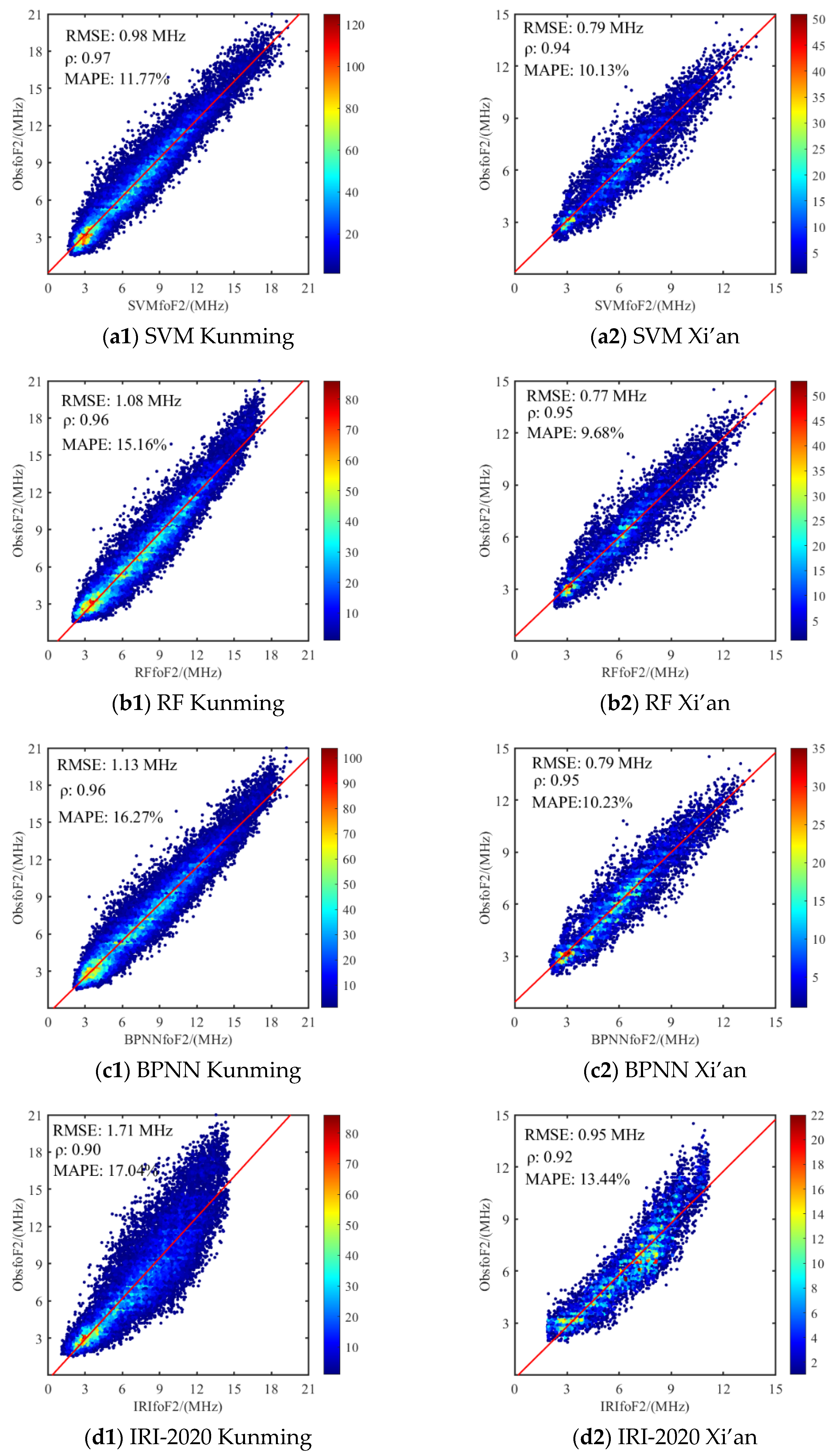
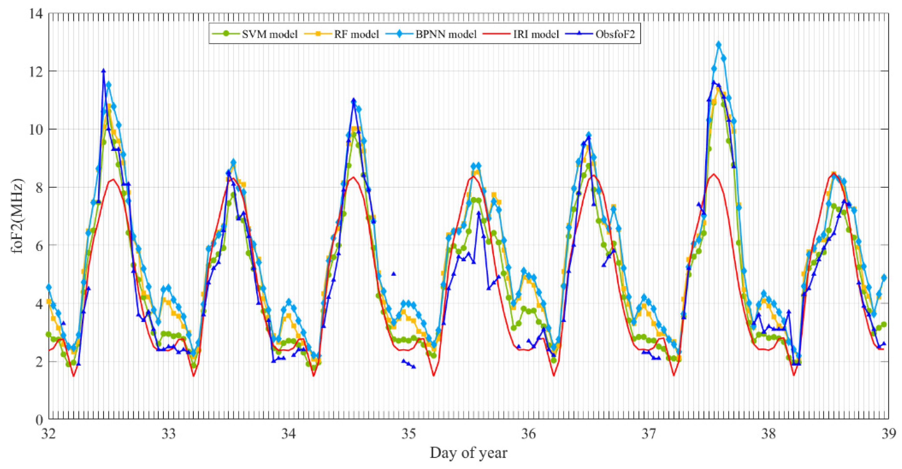
3.1. Model Performance and the foF2 Estimation Error

In this section, the performances of the three machine learning models are evaluated. And the IRI-2020 model is used as a reference model. Figure 6(a1,b1,c1,d1) present the results of observation and the machine learning model at Kunming station, and Figure 6(a2,b2,c2,d2) present the results at Xi’an station. The vertical coordinate ObsfoF2 denotes the foF2 observations, the horizontal coordinates SVMfoF2, RFfoF2, and BPNNfoF2 denote the foF2 estimations of the three machine learning models, respectively, and IRIfoF2 denotes the foF2 results of the IRI-2020 model, and the value of the colorbar denotes the number of samples.

As seen from Figure 6, the values of (RMSE, ρ, MAPE) of SVM, RF, BPNN and IRI-2020 at Kunming station are (0.98 MHz, 0.97,15.16%), (1.08 MHz, 0.96, 15.16%), (1.13 MHz, 0.96, 16.27%), and (1.71 MHz, 0.90, 17.04%), respectively. At Xi’an station, the values of (RMSE, ρ, MAPE) of SVM, RF, BPNN and IRI model are (0.79 MHz, 0.94, 10.13%), (0.77 MHz, 0.95, 9.68%), (0.79 MHz, 0.95, 10.23%), and (0.95 MHz, 0.92, 13.44%), respectively. Therefore, the three machine learning models have better performance to estimate foF2 than t IRI-2020.

At Kunming station, the SVM model outperforms the RF model and the BPNN model, and the BPNN model has the largest error among the three machine models. In addition, the results of RF and BPNN models are smaller than the observation results when the foF2 value was larger than 15 MHz while the SVM model results did not, which indicated that the foF2 values estimated by both the RF and BPNN models were easily underestimated when the foF2 value was larger, and this result implied that the generalization ability of the SVM model is better than that of the RF and BPNN models. At Xi’an station, the performances of the three machine learning models are comparable, and all the three machine learning models have higher accuracy than the corresponding models at Kunming station, which indicates that the machine learning models have better performance in mid-latitude regions than in low-latitude regions.

To further evaluate the performances of the three machine learning models, we calculate the RMSE and MAPE of the three models at five stations including Urumqi, Changchun, Beijing, Suzhou, and Lhasa. Unlike all the data of Kunming and Xi’an being used to test the models, only the data for the years 2009 and 2013 are used to test the models; the remaining data are used to train the models.

Table 3. RMSE and MAPE of foF2 for SVM, RF, BPNN and IRI-2020 models in 2009 and 2013.

Site Name	Year	SVM		RF		BPNN		IRI
		RMSE /MHz	MAPE	RMSE /MHz	MAPE	RMSE /MHz	MAPE	RMSE /MHz	MAPE
Urumqi	2009	0.44	8.34%	0.43	8.24%	0.47	8.76%	0.54	10.38%
	2013	0.46	6.18%	0.45	6.25%	0.47	6.41%	0.78	10.06%
Changchun	2009	0.41	7.57%	0.41	7.56%	0.45	8.54%	0.58	10.46%
	2013	0.50	6.45%	0.51	6.61%	0.50	6.50%	0.76	9.75%
Beijing	2009	0.48	8.06%	0.47	7.86%	0.52	8.91%	0.61	10.94%
	2013	0.50	6.29%	0.52	6.56%	0.51	6.42%	0.84	10.80%
Suzhou	2009	0.55	8.78%	0.51	8.29%	0.56	9.45%	1.00	17.20%
	2013	0.66	7.13%	0.70	7.48%	0.70	7.65%	1.30	15.90%
Lhasa	2009	0.62	9.52%	0.61	9.39%	0.66	10.45%	1.14	17.15%
	2013	0.74	7.83%	0.75	7.76%	0.77	8.43%	1.43	16.46%

lists RMSE and MAPE of foF2 for SVM, RF, BPNN and IRI-2020 models in 2009 (low solar activity year) and 2013 (high solar activity year). The five stations are listed in the table from high latitude to low latitude. As seen from Table 3, the values of RMSE and MAPE of the three machine learning models are all smaller than those of the IRI-2020 model. And there are no obvious differences between the three machine learning models. Both RMSE and MAPE values become larger with lower latitude (this phenomenon is not obvious for the similar latitudes of Urumqi and Changchun stations), and the values of RMSE in the year of 2013 (high solar activity year) are slightly larger than those in the year of 2009 (low solar activity year), while the values of MAPE in 2013 are slightly smaller than those in 2009. In addition, the values of RMSE and MAPE for these five stations are all smaller than those for Kunming and Xi’an stations. This is probably because the training data do not include the observational data at Kunming and Xi’an stations. In short, the foF2 values in the region of China can be well estimated by the three machine methods.

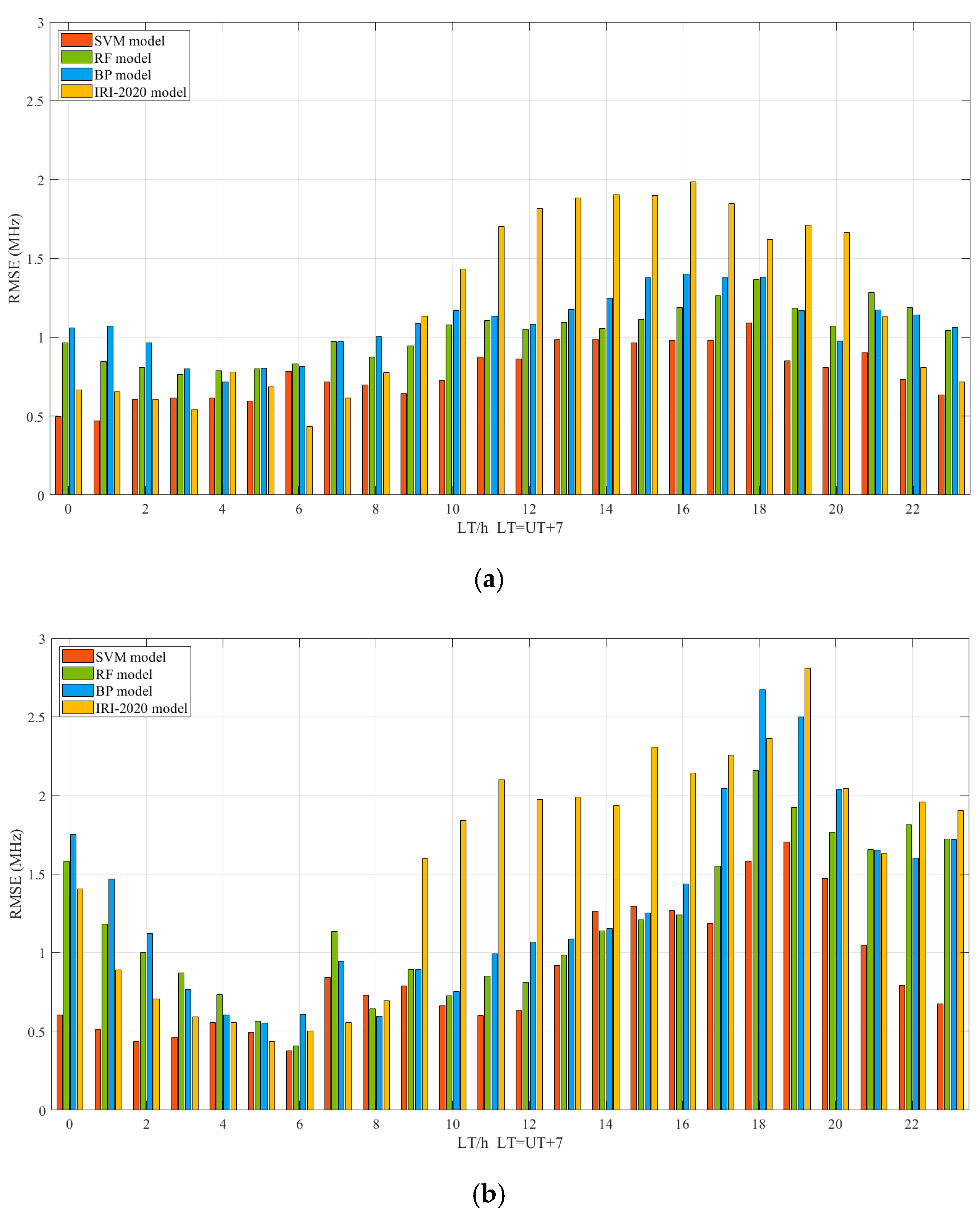
• Diurnal variations of foF2 RMSE values in machine learning models

Figure 7a,b show the hourly foF2 RMSE values of the three machine learning models, SVM, RF and BPNN at Kunming station for the low (2009) and high (2013) solar activity years. As seen from Figure 7a, the RMSE of SVM model has a minimum of 0.47 MHz at 1 LT and has a maximum of 1.09 MHz at 18 LT. The RMSE of the RF model has a minimum of 0.76 MHz at 3 LT and has a maximum of 1.37 MHz at 18 LT. The RMSE of the BPNN model has a minimum of 0.72 MHz at 4 LT and has a maximum of 1.40 MHz at 16 LT. Thus, the RMSE of the three machine learning models varies with local time and the RMSE of the SVM model has the smallest value of the three models. In addition, the RMSEs of the three machine learning models at 9 LT to 17 LT are obviously smaller than those of the IRI-2020 model.

As seen from Figure 7b, the RMSE of the SVM model has a minimum of 0.38 MHz at 6 LT and a maximum of 1.7 MHz at 19 LT. The RMSE of the RF model has a minimum of 0.41 MHz at 6 LT and a maximum of 2.16 MHz at 18 LT. The RMSE of the BPNN model has a minimum of 0.55 MHz at 5 LT and a maximum of 2.67 MHz at 18 LT. Thus, the RMSE of the three machine learning models varies with local time and the RMSEs of the SVM model are smaller than the other two models. The RMSEs of the three models are larger in the periods of 17 to 20 LT than those in the other periods. As seen from Figure 7, the diurnal variation in the RMSE of the SVM model is less obvious than that of both the RF and BPNN models. The RMSEs of the models from 3 LT to 16 LT of 2013 are close to or slightly smaller than those values from 2009, while the RMSEs of models from 17 LT to 23 LT and 0 LT to 1 LT of 2013 are much larger than the values from 2009, especially for RF and BP models. Overall, the RMSEs of the SVM model at Kunming station are the smallest of the three models, both for 2009 and 2013.

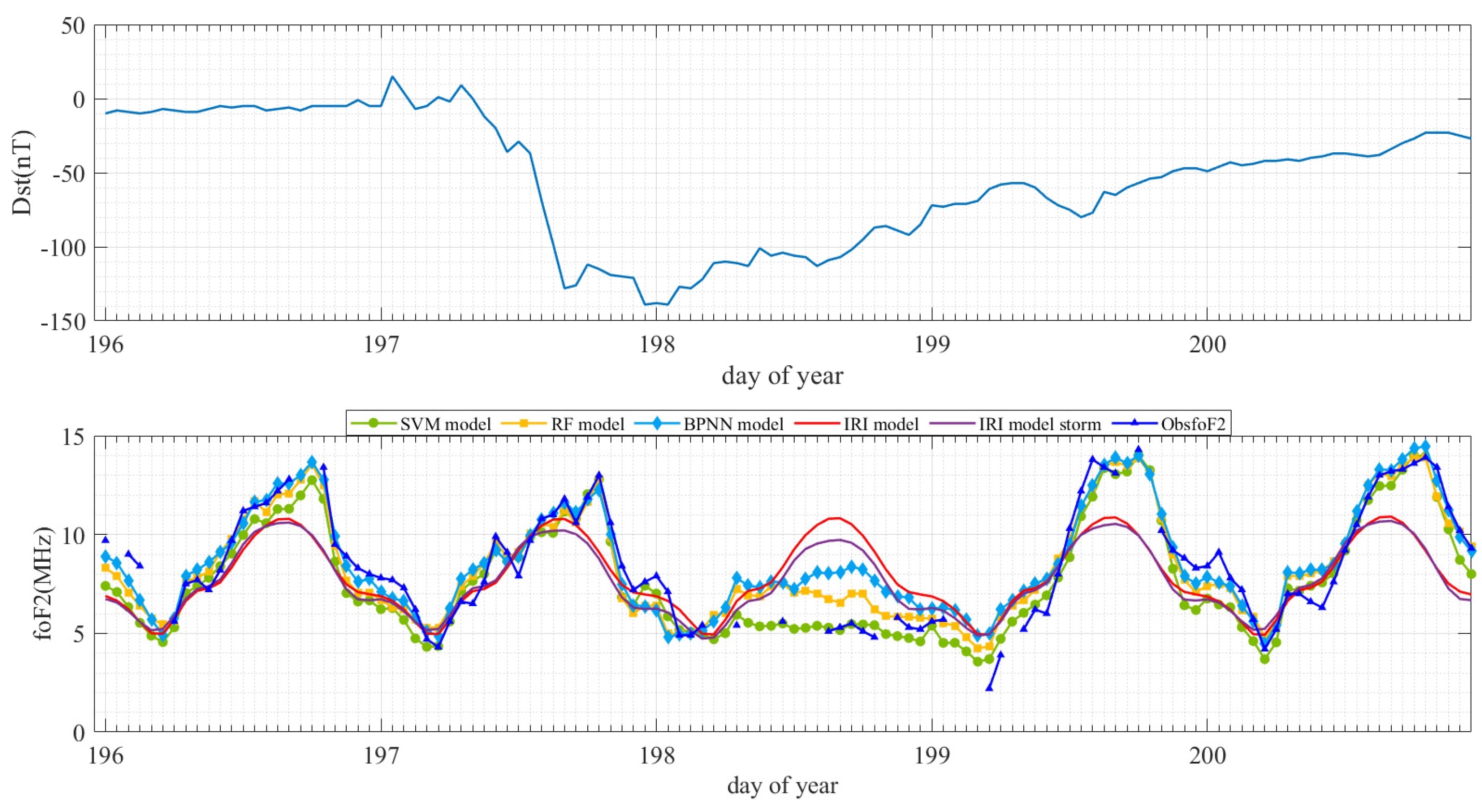
• Performance evaluation of the models in estimating foF2 under quiet and disturbed ionospheric conditions

Figure 8 shows the values of foF2 versus day of year obtained by models of SVM, RF, BPNN, IRI, and observations at Kunming station, respectively, during the magnetically quiet days (1–7 February 2009). The discontinuity of the data in the figure is caused by the missing foF2 observational data. As seen in Figure 8, the three machine learning models have comparable accuracy and the model results of foF2 are close to the observation results during the daytime when the foF2 values are larger, while the IRI-2020 model has a large bias. Notably, the IRI model shows no discernible variation in its temporal curves between consecutive days, demonstrating that its outputs reflect climatological behavior based on smoothed F10.7 indices rather than capturing short-term disturbances. At night, when the foF2 values are small, the SVM model still captures the foF2 variation better than the RF and BPNN models. Overall, all three machine learning models can represent the diurnal variation in foF2, and the SVM model performs best.

To evaluate the performance of foF2 estimation models during geomagnetic disturbances, we present a comparative analysis between observational data from Kunming station and the predictions of SVM, RF, BPNN, and IRI models during the period of 14–18 July 2012 (see Figure 9). The upper panel of Figure 9 illustrates the occurrence of an intense geomagnetic storm event, while the lower panel displays the temporal comparison between model predictions and measured values. Data gaps in the figure are the result of missing foF2 observations. Additionally, we show the IRI-2020 model estimations with both disabled (red curve) and enabled (purple curve) storm options [32]. The lower panel demonstrates that while the IRI-2020 model with the storm option activated responds to geomagnetic disturbances (manifested as foF2 reduction), its estimates still exhibit significant deviations from observations, indicating limited capability in capturing foF2 variations during geomagnetic disturbances.

Figure 9 reveals that all three machine learning models (SVM, RF, BPNN) capture the foF2 variations during geomagnetic disturbances to varying degrees. For this particular event, the SVM model appears to perform best, showing the closest agreement with observations. However, a single event cannot conclusively demonstrate that SVM yields the smallest errors during geomagnetic disturbances. Therefore, we conducted a further evaluation using Kunming station’s foF2 data from 2008 to 2013. By employing the Dst index, we identified 156 geomagnetic storm events during this period. Figure 10 presents error distribution histograms for the three machine learning models during disturbed conditions, where the x-axis represents the difference between model estimates and observations, and the y-axis shows probability density. The black dashed line indicates zero error, while three additional dashed lines (μ_A = −0.35 MHz, μ_B = 0.19 MHz, μ_C = 0.42 MHz) represent mean error lines for the SVM, RF, and BPNN models, respectively. For comprehensive performance assessment during geomagnetic disturbances,

Table 4. Performance comparison of SVM, RF, and BPNN in foF2 estimation during geomagnetic storms (2008–2013, Kunming station).

Model	Mean (MHz)	Standard Deviation (MHz)	Skewness	Kurtosis	Root Mean Square Error (MHz)
SVM	−0.35	1.07	−0.47	3.73	1.13
RF	0.19	1.09	−0.40	3.41	1.11
BPNN	0.42	1.08	−0.27	3.42	1.16

provides statistical metrics including mean error, standard deviation, skewness, kurtosis, and root mean square error.

The comparative performance analysis presented in Table 4 reveals that during geomagnetic disturbance events, the RMSE values for the three machine learning models were measured at 1.13 MHz (SVM), 1.11 MHz (RF), and 1.16 MHz (BPNN). Notably, these error metrics demonstrate close agreement with the comprehensive RMSE derived from the complete 2008–2013 observational dataset at Kunming station (Figure 6), thereby confirming that all three computational approaches effectively characterize foF2 variations under disturbed geomagnetic conditions.

As evidenced by the comparative results in Figure 10 and Table 4, the RF algorithm exhibits statistically superior performance relative to both SVM and BPNN implementations during geomagnetic disturbances. The statistical analysis yields two significant observations: first, the consistently negative skewness coefficients across all models indicate a systematic underestimation bias in their predictive outputs; second, the leptokurtic distributions (kurtosis > 3) suggest non-negligible probabilities of extreme prediction errors. These statistical characteristics provide a robust explanation for the limited number of high-magnitude error outliers apparent in the model prediction versus observation scatter plot (Figure 6).

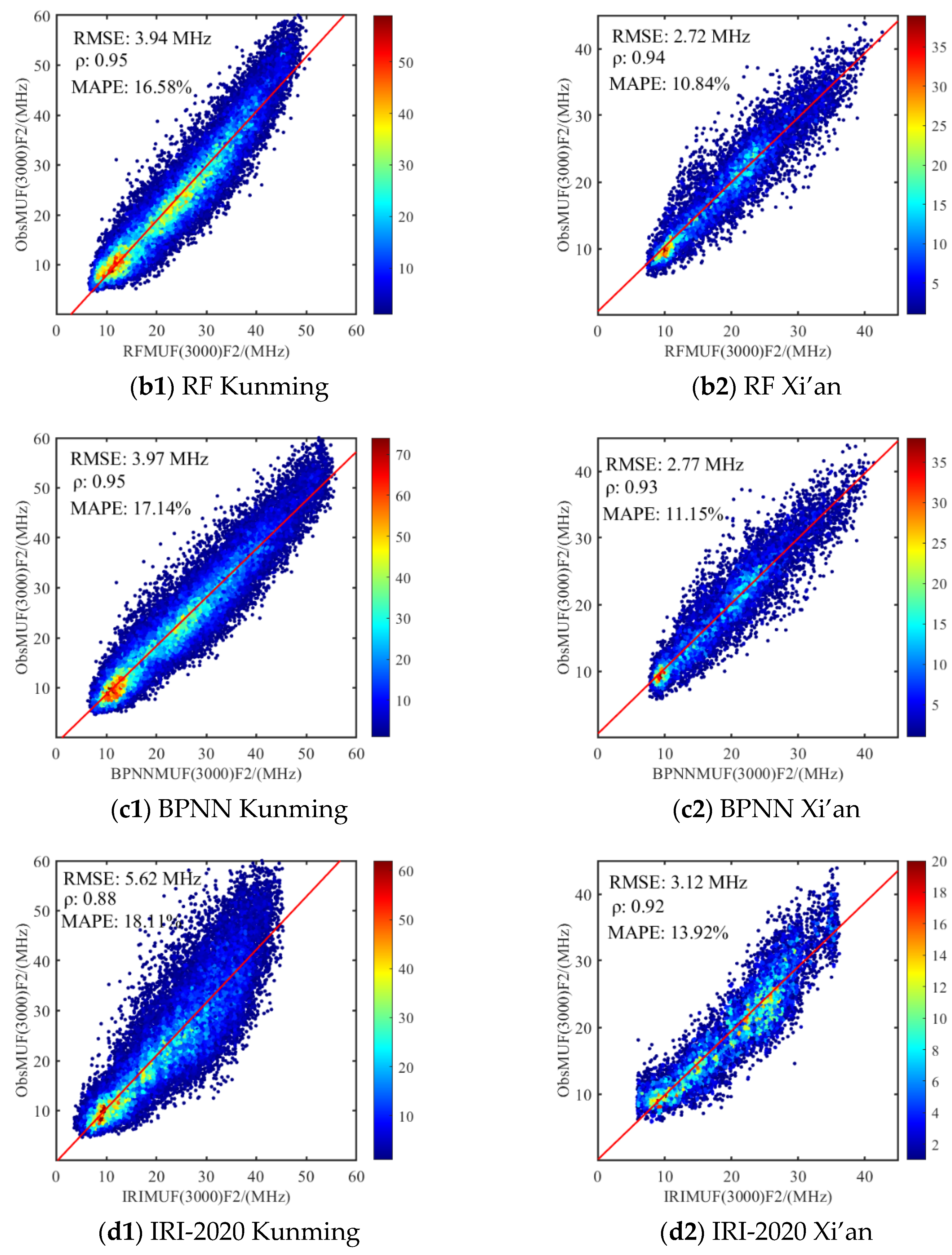
3.2. Estimation Results of MUF(3000)F2 and Model Performance Evaluation

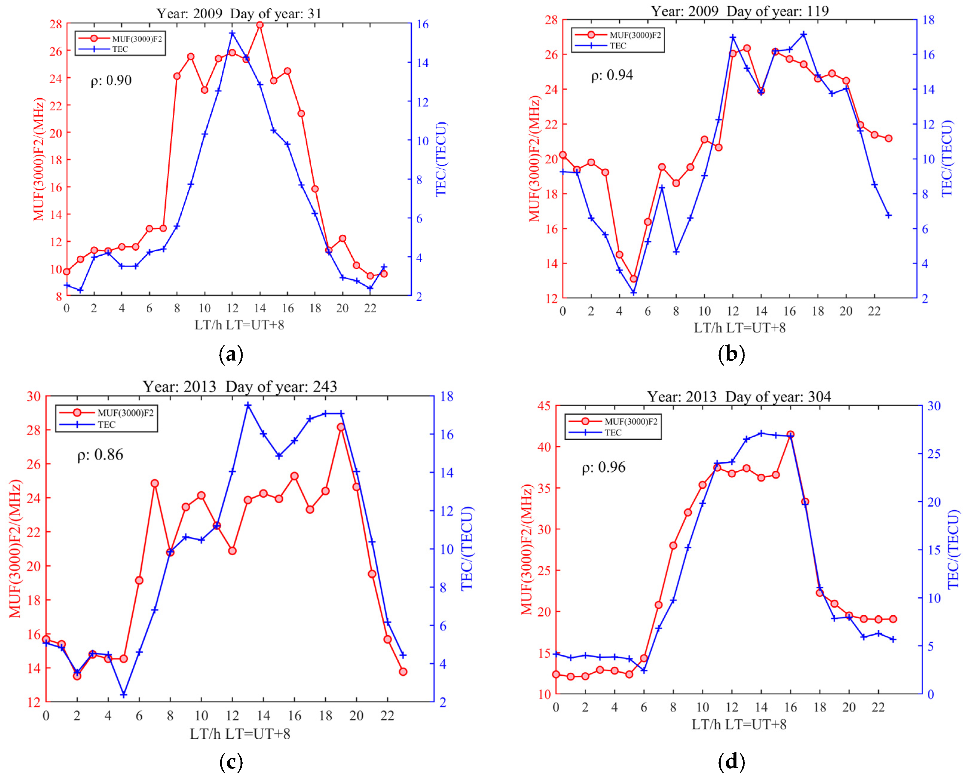
3.2.1. Relationship Between MUF(3000)F2 and TEC

The purpose of this section is to study the correlation between MUF(3000)F2 and TEC because MUF(3000)F2 can only estimate by machine learning models with TEC if there exists correlation between the two parameters. It should be noted that the data used in this section are not model results but observation results by ionosonde and GNSS receivers. Figure 11 shows the diurnal variations in MUF(3000)F2 and TEC at Beijing station (40.11°N, 116.28°E). The four days of data presented in Figure 11 are randomly selected in different seasons and different solar activity levels, and ρ is the correlation coefficient between MUF(3000)F2 and TEC. As seen from Figure 11a–d, it is obvious that there is a very significant correlation between the MUF(3000)F2 observed by the ionosonde and the TEC observed by the corresponding GNSS receiver, and the correlation coefficients are all greater than 0.8, and most of them are above 0.9, which proves the feasibility of using TEC to estimate MUF(3000)F2 in this paper.

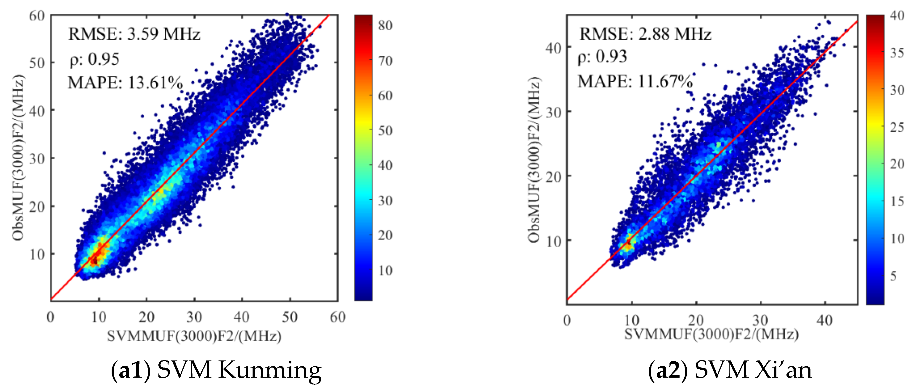
3.2.2. The MUF(3000)F2 Estimation Error and Model Performance

In this section, the performances of the three machine learning models are evaluated. And the IRI-2020 model is used as a reference model. Figure 12a1,b1,c1,d1 present the results of the observation and machine learning model at Kunming station, and Figure 12a2,b2,c2,d2 present the results at Xi’an station. The vertical coordinate ObsMUF(3000)F2 denotes the MUF(3000)F2 observations, the horizontal coordinates SVMMUF(3000)F2, RFMUF(3000)F2, and BPNNMUF(3000)F2 denote the MUF(3000)F2 estimations of the three machine learning models, respectively, and IRIMUF(3000)F2 denotes the MUF(3000)F2 results of the IRI-2020 model, and the value of the colorbar denotes the number of samples.

As seen from Figure 12, the values of the (RMSE, ρ, and MAPE) of SVM, RF, BPNN and IRI-2020 at Kunming station are (3.59 MHz, 0.95, 13.61%), (3.94 MHz, 0.95, 16.58%), (3.97 MHz, 0.95, 17.14%), and (5.62 MHz, 0.88, 18.11%), respectively. At Xi’an station, the values of (RMSE, ρ, and MAPE) of SVM, RF, BPNN and IRI models are (2.88 MHz, 0.93, 11.67%), (2.72 MHz, 0.94, 10.84%), (2.77 MHz, 0.93, 11.15%), and (3.12 MHz, 0.92, 13.92%), respectively. Therefore, the three machine learning models give a better performance to estimate foF2 than t IRI-2020.

As with the foF2 estimation, the SVM model outperforms the RF model and the BPNN model at Kunming station, and the BPNN model has the largest error of the three machine models. In addition, the results from the RF and BPNN models were smaller than the observation results when the MUF(3000)F2 value was larger than 45 MHz, while the SVM model results were not, which indicated that the MUF(3000)F2 values estimated by both the RF and BPNN models were easily underestimated when the MUF(3000)F2 value was larger, and this result implied that the generalization ability of the SVM model is better than that of the RF and BPNN models. At Xi’an station, the performances of the three machine learning models are comparable, and all the three machine learning models have higher accuracy than the corresponding models at Kunming station, which indicates that the machine learning models have better performance in mid-latitude regions than in low-latitude regions.

Table 5. RMSE and MAPE of MUF(3000)F2 for SVM, RF, BPNN and IRI-2020 models in 2009 and 2013.

Site Name	Year	SVM		RF		BPNN		IRI
		RMSE /MHz	MAPE	RMSE /MHz	MAPE	RMSE /MHz	MAPE	RMSE /MHz	MAPE
Urumqi	2009	1.73	9.88%	1.70	9.71%	1.81	10.45%	2.04	11.51%
	2013	1.78	7.59%	1.73	7.42%	1.81	7.64%	2.48	10.45%
Changchun	2009	1.72	9.10%	1.70	9.04%	1.79	9.78%	2.44	12.62%
	2013	1.88	7.69%	1.87	7.70%	1.92	7.85%	2.48	11.32%
Beijing	2009	1.93	9.69%	1.86	9.36%	1.96	10.01%	2.38	12.36%
	2013	1.91	7.64%	1.88	7.61%	1.92	7.74%	2.72	11.33%
Suzhou	2009	2.35	10.94%	2.15	10.10%	2.34	10.90%	3.45	17.35%
	2013	2.43	8.69%	2.46	8.76%	2.50	8.84%	4.12	16.68%
Lhasa	2009	2.59	11.30%	2.50	10.91%	2.69	12.17%	4.04	17.98%
	2013	2.73	9.68%	2.70	9.33%	2.76	9.81%	4.53	17.82%

lists RMSE and MAPE of SVM, RF, BPNN and IRI-2020 models in 2009 (low solar activity year) and 2013 (high solar activity year). The five stations are listed in the table from high latitude to low latitude. As seen in Table 5, the values of RMSE and MAPE for the three machine learning models are all smaller than those for the IRI-2020 model. And there are no obvious differences between the three machine learning models. Both RMSE and MAPE values become larger with lower latitude except Urumqi, and the values of RMSE in the year 2013 (high solar activity year) are slightly larger than those in the year 2009 (low solar activity year), while the values of MAPE in 2013 are slightly smaller than those in 2009. In addition, the values of RMSE and MAPE for these five stations are all smaller than those for Kunming and Xi’an stations. This is probably because the training data do not include the observational data at Kunming and Xi’an stations. In short, MUF(3000)F2 values in the region of China can be well estimated by the three machine methods.

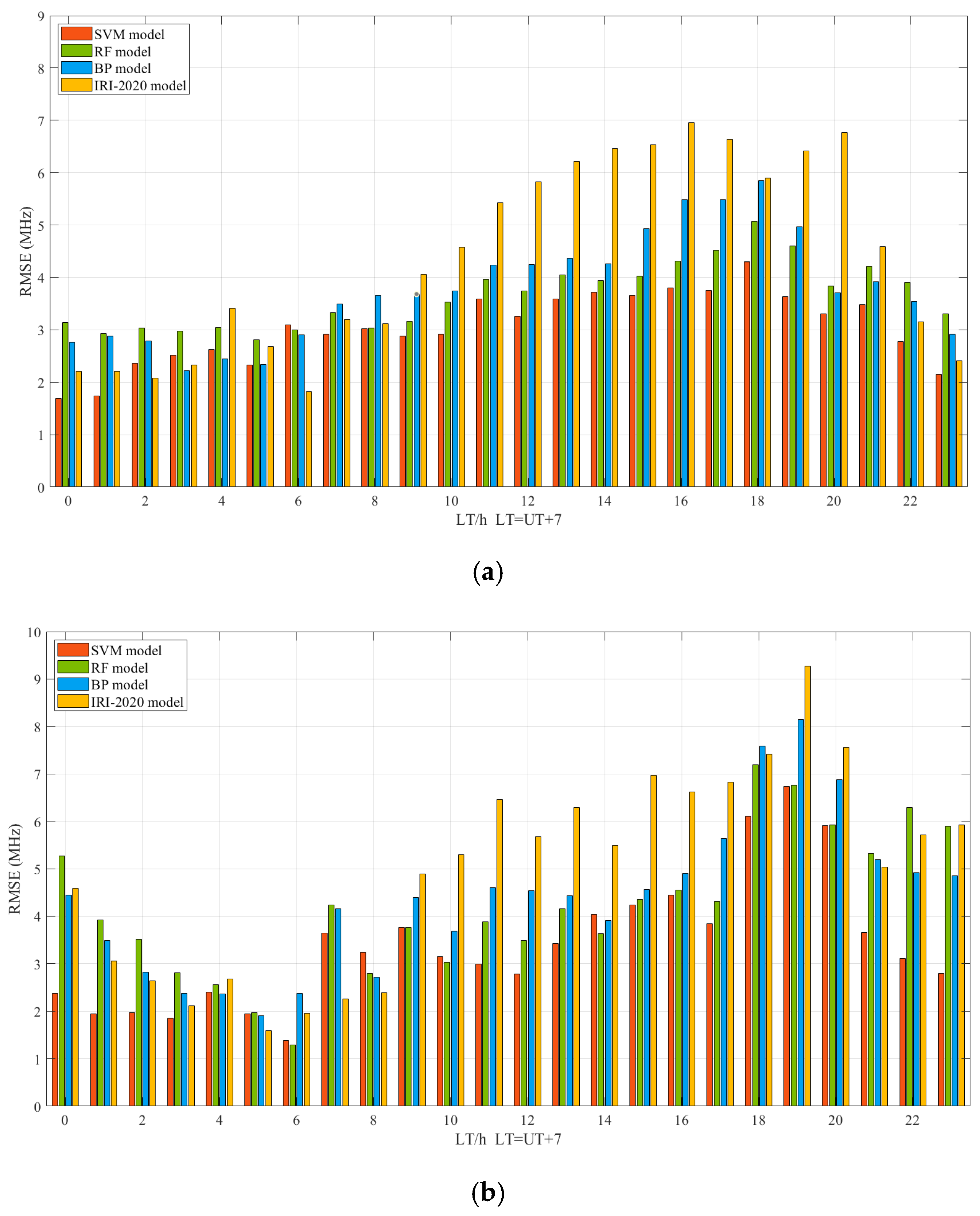
• Diurnal variations of MUF(3000)F2 RMSE values in RMSE of the machine learning models

Figure 13a,b show the hourly MUF(3000)F2 RMSE values of the three machine learning models (SVM, RF, BPNN) and IRI-2020 model at Kunming station for low (2009) and high (2013) solar activity years. As seen from Figure 13a, the RMSE of the SVM model has a minimum of 1.69 MHz at 0 LT and has a maximum of 4.29 MHz at 18 LT. The RMSE of the RF model has a minimum of 2.80 MHz at 0 LT and has a maximum of 5.07 MHz at 18 LT. The RMSE of the BPNN model has a minimum of 2.22 MHz at 5 LT and has a maximum of 5.85 MHz at 18 LT. Thus, the RMSE of the three machine learning models varies with local time and the RMSE of the SVM model has the smallest value of the three models. Furthermore, the RMSE of the three machine learning models at 9 LT to 17 LT are obviously smaller than those of the IRI-2020 model.

As seen from Figure 13b, the RMSE of the SVM model has a minimum of 1.38 MHz at 6 LT and a maximum of 6.73 MHz at 19 LT. The RMSE of the RF model has a minimum of 1.29 MHz at 6 LT and a maximum of 7.20 MHz at 18 LT. The RMSE of the BPNN model has a minimum of 1.90 MHz at 6 LT and a maximum of 8.14 MHz at 19 LT. Thus, the RMSE of the three machine learning models varies with local time and the RMSEs of the SVM model are smaller than the other two models. The RMSEs of the three models are larger in the periods of 18 to 20 LT than those in the other periods. As seen from Figure 13, the diurnal variation in RMSE of the SVM model is less obvious than that of both the RF and the BPNN models. The RMSEs of the models from 3 LT to 16 LT of 2013 are close to or slightly smaller than those values for 2009, while the RMSEs of models from 18 LT to 23 LT and 0 LT to 1 LT for 2013 are much larger than those values for 2009, especially for RF and BP models. Overall, the RMSEs of the SVM model at Kunming station are the smallest of the three models, both for 2009 and 2013.

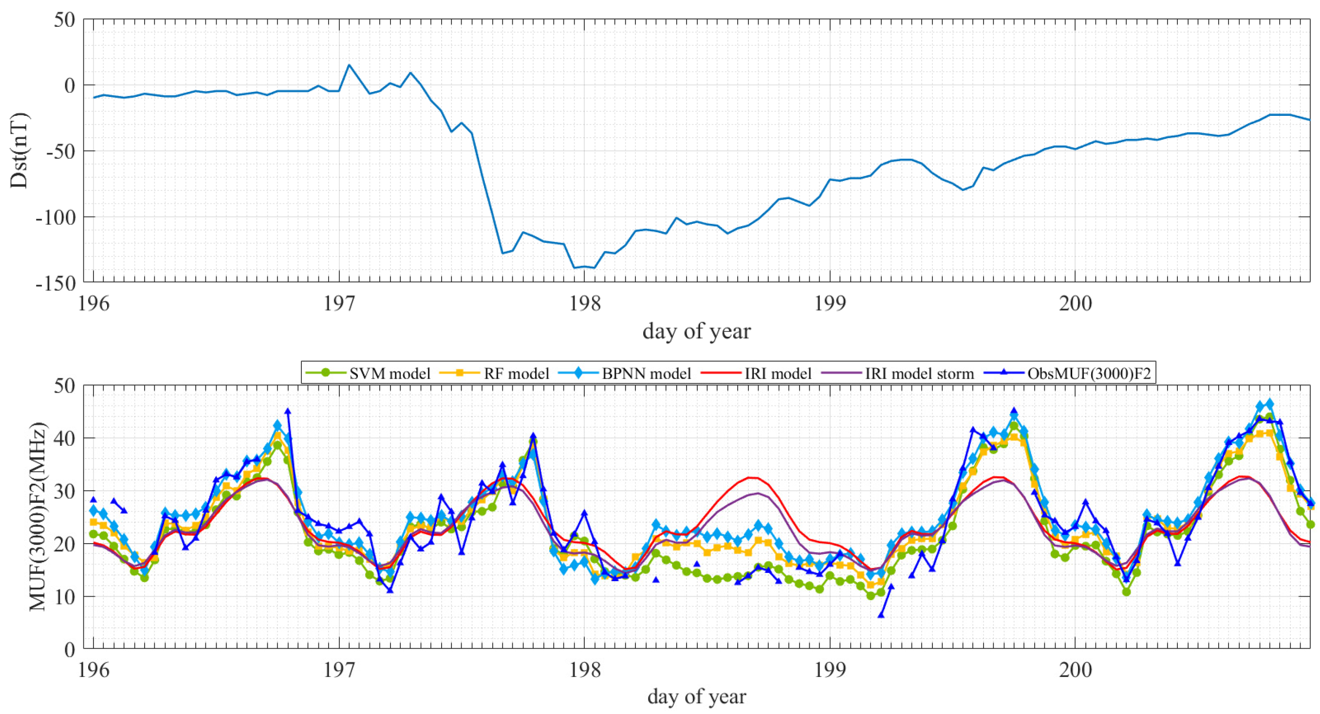
• Performance evaluation of the models in estimating MUF(3000)F2 under quiet and disturbed ionospheric conditions

Figure 14 shows the values of MUF(3000)F2 versus day of year obtained by the models of SVM, RF, BPNN, IRI, and observations at Kunming station, respectively, during the magnetically quiet days (1–7 February 2009). The discontinuity of the data in the figure is caused by the missing of foF2 observational data. As seen in Figure 14, the three machine learning models have comparable accuracy and the model results of MUF(3000)F2 are close to the observation results during the daytime when the MUF(3000)F2 values are larger, while the IRI-2020 model has a large bias. At night, when the MUF(3000)F2 values are small, the SVM model still captures the MUF(3000)F2 variation better than the RF and BPNN models. Overall, all the three machine learning models can represent the diurnal variation in foF2, and the SVM model performs best.

To demonstrate the performance of MUF(3000)F2 estimation models during geomagnetic disturbances, we present a comparative analysis of observational data from Kunming ionosonde station with predictions from SVM, RF, BPNN, and IRI models during the intense geomagnetic storm event from 14 to 18 July 2012, (see Figure 15). The upper panel of Figure 15 shows the geomagnetic storm conditions, while the lower panel displays the temporal variations in modeled versus observed values. Data gaps in the figure result from missing MUF(3000)F2 observations. Additionally, we show IRI-2020 model outputs with both disabled (red curve) and enabled (purple curve) storm options. The lower panel reveals that while the storm-enabled IRI-2020 responds to geomagnetic activity (manifested as MUF(3000)F2 depression), its estimates exhibit significant deviations from observations, indicating limited capability in capturing storm-time MUF(3000)F2 variations. Figure 15 demonstrates that all three machine learning models (SVM, RF, and BPNN) capture MUF(3000)F2 variations during this disturbance event to varying degrees, with SVM showing the closest agreement to observations. However, a single event cannot conclusively establish SVM’s superior performance. Therefore, we conducted a comprehensive evaluation using Kunming station’s MUF(3000)F2 data from 2008 to 2013. We identified 156 geomagnetic storm events using Dst index thresholds during this period.

Figure 16 presents error distribution histograms for the three ML models during disturbed conditions, with the x-axis showing model–observation differences (MHz) and the y-axis representing probability density. The black dashed line indicates zero-error reference, while μ_A = −0.98 MHz, μ_B = 0.26 MHz, and μ_C = 1.54 MHz denote mean errors for SVM, RF, and BPNN, respectively. For a thorough assessment,

Table 6. Performance comparison of SVM, RF, and BPNN in MUF(3000)F2 estimation during geomagnetic storms (2008–2013, Kunming station).

Model	Mean (MHz)	Standard Deviation (MHz)	Skewness	Kurtosis	Root Mean Square Error (MHz)
SVM	−0.98	3.87	−0.20	3.45	3.99
RF	0.26	4.10	−0.30	3.39	4.10
BPNN	1.54	3.89	−0.09	3.41	4.19

summarizes key statistics: mean error, standard deviation, skewness, kurtosis, and RMSE during storm events.

The comparative performance analysis presented in Table 6 reveals that during geomagnetic disturbance events, the RMSE values for the three machine learning models were measured at 3.99 MHz (SVM), 4.10 MHz (RF), and 4.19 MHz (BPNN). While these disturbance-period RMSE values exhibit a modest elevation compared to the comprehensive RMSE derived from the complete 2008–2013 observational dataset at Kunming station (Figure 12), the overall proximity of these metrics suggests that all three computational approaches effectively characterize MUF(3000)F2 variations under disturbed geomagnetic conditions.

The analysis results from Figure 16 and Table 6 demonstrate the following:

(1) RF exhibits minimal systematic bias but poorest stability (highest standard deviation).

(2) SVM shows better stability but greater systematic bias.

(3) All models demonstrate negative skewness (skew < 0), indicating systematic underestimation.

(4) Leptokurtic distributions (kurtosis > 3) suggest non-negligible probabilities of extreme errors.

4. Discussion

There has been much research on building foF2 estimation models based on the strong correlation between TEC and foF2. Krankowski et al., 2007, [33] proposed a method to estimate foF2 from GPS VTEC observations. They made full use of the computational relationship between foF2, VTEC, and ionospheric equivalent slab thickness (τ), and implemented the TEC-to-foF2 conversion using the ionospheric equivalent slab thickness (τ) obtained from an empirical model. However, obtaining the ionospheric equivalent slab thickness (τ) model is not easy. Ssessanga et al., 2014 [34] proposed a method to obtain ionospheric foF2 from GPS VTEC in the South African region using polynomial functions. This method is only applicable for foF2 estimation when Kp is less than four and is not suitable for estimating foF2 during geomagnetic disturbances. Moreover, the polynomial coefficients are closely related to the time period, month, and geographic location, requiring the selection of appropriate model coefficients based on different times and geographic locations. Otugo et al., 2019 [4] used a neural network to build an foF2 estimation model. The model uses TEC, day of the year (DOY), local time (LT), sunspot number (SSN), and the geomagnetic storm index (Dst) as inputs to estimate foF2 values, achieving good results. This study focused on analyzing the influence of local time, season, and solar and geomagnetic activity on the TEC–foF2 relationship to determine the inputs for the neural network model, but did not provide a detailed evaluation of the neural network model’s performance, such as analyzing the model’s performance during geomagnetically quiet and disturbed periods. This paper proposes a machine learning-based method to estimate foF2 and MUF(3000)F2 using TEC observations. The study focuses on analyzing and comparing the performance of different machine learning algorithms (BP, RF, SVM), and it separately analyzes the performance differences of the three models under varying latitudes, local times, and solar activity levels, providing a comprehensive evaluation of the strengths and weaknesses of each model for guiding engineering applications. The study found that the RMSE during solar minimum years is smaller than during solar maximum years, and the RMSE in mid-latitude regions is smaller than in low-latitude regions. The RMSE in the evening is larger, while the RMSE in the early morning is smaller; this difference is especially significant during solar maximum years. Furthermore, the study reveals that all three machine learning models demonstrate varying capabilities in capturing storm-time variations in both foF2 and MUF(3000)F2. For foF2 estimation, the RF model exhibits minimal systematic bias (0.19 MHz), showing closest agreement with observational data. Regarding MUF(3000)F2 estimation, while the RF model exhibits minimal systematic bias (0.26 MHz), it displays inferior stability as indicated by its highest standard deviation (4.10 MHz). Conversely, the SVM model, despite showing greater systematic bias (−0.98 MHz), provides optimal stability with the lowest standard deviation (3.87 MHz) among the tested models.

This paper analyzes for the first time the correlation between TEC and MUF(3000)F2, demonstrating the feasibility of estimating MUF(3000)F2 using TEC. By utilizing the strong correlation between TEC and MUF(3000)F2, an estimation model for MUF(3000)F2 is established. Due to the limited ionospheric data available, this study did not construct a global foF2 estimation model. However, if ionospheric data from different regions around the world can be obtained, global foF2 and MUF(3000)F2 maps can be generated through global TEC maps.

5. Conclusions

In this paper, three machine learning models based on SVM, RF and BPNN algorithms are established to estimate the ionospheric foF2 and MUF(3000)F2 from TEC observations. Machine learning models are trained using data from nine stations in the China region, Mohe, Urumqi, Changchun, Beijing, Suzhou, Wuhan, Lhasa, Guangzhou and Sanya, except for 2009 and 2013. Data from Kunming station (2007–2013), Xi’an (2010–2011), Urumqi, Changchun, Beijing, Suzhou, and Lhasa (2009 and 2013) are used as test sets to evaluate the performance of the models. The work of this paper can be concluded as follows.

(1) In estimating foF2 (MUF(3000)F2), the SVM, RF, BPNN, and IRI-2020 model RMSEs at Kunming station are 0.98 MHz (3.59 MHz), 1.08 MHz (3.94 MHz), 1.13 MHz (3.97 MHz), and 1.71 MHz (5.62 MHz), respectively, while those values at Xi’an station are 0.79 MHz (2.88 MHz), 0.77 MHz (2.72 MHz), 0.79 MHz (2.77 MHz), and 0.95 MHz (3.12 MHz), respectively. The results show all the machine learning models established in this paper perform better than IRI-2020 for both low-latitude (Kunming station) and mid-latitude (Xi’an), and values of RMSEs of foF2 models are smaller than those of MUF(3000)F2. For foF2 estimation, RMSE values at Kunming and Xi’an stations are, respectively, decreased by ~38% and ~18%, compared to those of IRI-2020. And for MUF(3000)F2 estimation, those values are respectively decreased by ~26% and ~11%, compared to those of IRI-2020.

(2) When the machine learning model performances were evaluated using datasets at Kunming and Xi’an stations, the data of which were not involved in training, it was found that the SVM model had the best performance and the smallest error in the low-latitude region followed by the RF model and the BPNN model. However, in the mid-latitude region, there was little difference between the performances of the three machine learning models. When the performances of the machine learning models are evaluated using the dataset of stations with partial year data involved in training (five stations, such as Urumqi and Changchun), it was found that the performance difference between the three machine learning models was not significant and the error values were smaller than those of stations of which data were not involved in training.

(3) The RMSE of the three machine learning models varies with local time and the RMSEs of the SVM model are smaller than the other two models. The RMSEs of the three models are larger in the periods of 17 to 20 LT than those in the other periods. The RMSE of the SVM model at Kunming station is the smallest of the three models both for 2009 and 2013. The diurnal variation in RMSE of the SVM model is less obvious than that of both RF and BPNN models. And this indicates that the generalization ability of the SVM model is stronger than that of the RF model and the BPNN model. In addition, the RMSE values of low solar activity years are smaller than those of high solar activity years. The RMSE values in mid-latitude regions are smaller than those in low-latitude regions. The RMSE values are larger in the evening and smaller in the wee hours, and this difference is especially significant in high solar activity years.

(4) A comprehensive evaluation of three machine-learning models was conducted using observational data from 156 geomagnetic storm events recorded at the Kunming station between 2008 and 2013. The results indicate that during geomagnetic disturbances, the RF model performed best in estimating foF2, exhibiting the smallest systematic bias. However, for MUF(3000)F2 estimation, although the RF model still showed the least systematic bias, its stability was relatively poor, whereas the SVM model, despite having a larger systematic bias, demonstrated superior stability. Therefore, for foF2 estimation during geomagnetic disturbances, the RF model is recommended. For MUF(3000)F2 estimation, the choice between models depends on the priority: if stability is prioritized, the SVM model is preferable, whereas if minimizing systematic bias is the primary concern, the RF model should be selected.

This study proposes a machine learning-based method for estimating foF2 and MUF(3000)F2 by TEC observations. This method provides machine learning models that can be integrated into GNSS receivers, enabling GNSS receivers to obtain foF2 and MUF(3000)F2 values while observing TEC, which will be of great importance for areas where ionosondes are lacking or unavailable. In addition, the TEC data obtained by a GNSS receiver have good integrity and do not easily go missing, while the observational data obtained by ionosonde easily go missing and have poor data integrity. And this method can also estimate the missing ionosonde foF2 and MUF(3000)F2 data by TEC to supplement the ionosonde observational data.

References

1. Buonsanto, M.J. Ionospheric storms—A review. Space Sci. Rev. 1999, 88, 563–601. [Google Scholar] [CrossRef]
2. Siddique, H.; Tahir, A.; Gul, I.; Waris, B.B.; Ameen, M.A.; Talha, M.; Ali, M.S.; Ansari, A.; Javaid, S. Estimation of MUF(3000)F2 using Earth-ionosphere geometry for Karachi and Multan, Pakistan. Adv. Space Res. 2021, 68, 4646–4657. [Google Scholar] [CrossRef]
3. Spalla, P.; Cairolo, L. TEC and foF2 comparison. Ann. Geophys. 1994, 37, 929–938. [Google Scholar] [CrossRef]
4. Otugo, V.N.; Okoh, D.; Okujagu, C.; Onwuneme, S.; Rabiu, B.; Uwamahoro, J.; Habarulema, J.B.; Tshisaphungo, M.; Ssessanga, N. Estimation of Ionospheric Critical Plasma Frequencies From GNSS-TEC Measurements Using Artificial Neural Networks. Space Weather 2019, 17, 1329–1340. [Google Scholar] [CrossRef]
5. Hernández-Pajares, M.; Juan, J.M.; Sanz, J. Neural network modeling of the ionospheric electron content at global scale using GPS data. Radio Sci. 1997, 32, 1081–1089. [Google Scholar] [CrossRef]
6. Poole, A.W.V.; McKinnell, L.-A. On the predictability of foF2 using neural networks. Radio Sci. 2000, 35, 225–234. [Google Scholar] [CrossRef]
7. Oyeyemi, E.O.; Poole, A.W.V.; McKinnell, L.A. On the global model for foF2 using neural networks. Radio Sci. 2005, 40, 1–15. [Google Scholar] [CrossRef]
8. Oyeyemi, E.O.; Poole, A.; McKinnell, L.A. On the global short-term forecasting of the ionospheric critical frequency foF2 up to 5 hours in advance using neural networks. Radio Sci. 2005, 40, 5347–5356. [Google Scholar] [CrossRef]
9. Nakamura, M.I.; Maruyama, T.; Shidama, Y. Using a neural network to make operational forecasts of ionospheric variations and storms at Kokubunji. Earth Planet Space 2007, 59, 1231–1239. [Google Scholar] [CrossRef]
10. Leandro, R.F.; Santos, M.C. A neural network approach for regional vertical total electron content modelling. Stud. Geophys. Geod. 2007, 51, 279–292. [Google Scholar] [CrossRef]
11. Habarulema, J.B.; Mckinnell, L.A.; Cilliers, P.J. Prediction of global positioning system total electron content using Neural Networks over South Africa. J. Atmos. Solar-Terr. Phys. 2007, 69, 1842–1850. [Google Scholar] [CrossRef]
12. Habarulema, J.B.; McKinnell, L.A. Investigating the performance of neural network backpropagation algorithms for TEC estimations using South African GPS data. Ann. Geophys. 2012, 30, 857–866. [Google Scholar] [CrossRef]
13. Sai Gowtam, V.; Tulasi Ram, S. An Artificial Neural Network based Ionospheric Model to predict NmF2 and hmF2 using long-term data set of FORMOSAT-3/COSMIC radio occultation observations: Preliminary results. J. Geophys. Res. Space 2007, 122, 743–755. [Google Scholar] [CrossRef]
14. Song, R.; Zhang, X.; Zhou, C.; Liu, J.; He, J. Predicting TEC in China based on the neural networks optimized by genetic algorithm. Adv. Space Res. 2018, 62, 745–759. [Google Scholar] [CrossRef]
15. Fan, J.; Liu, C.; Lv, Y.; Han, J.; Wang, J. A Short-Term Forecast Model of foF2 Based on Elman Neural Network. Appl. Sci. 2019, 9, 2782. [Google Scholar] [CrossRef]
16. Zhao, J.; Li, X.; Liu, Y.; Wang, X.; Zhou, C. Ionospheric foF2 disturbance forecast using neural network improved by a genetic algorithm. Adv. Space Res. 2019, 63, 4003–4014. [Google Scholar] [CrossRef]
17. Xia, G.; Liu, Y.; Wei, T.; Wang, Z.; Huang, W.; Du, Z.; Zhang, Z.; Wang, X.; Zhou, C. Ionospheric TEC forecast model based on support vector machine with GPU acceleration in the China region. Adv. Space Res. 2021, 68, 1377–1389. [Google Scholar] [CrossRef]
18. Sun, W.; Xu, L.; Huang, X.; Zhang, W.; Yuan, T.; Chen, Z.; Yan, Y. Forecasting of ionospheric vertical total electron content (TEC) using LSTM networks. In Proceedings of the 2017 International Conference on Machine Learning and Cybernetics (ICMLC), Ningbo, China, 9–12 July 2017; Volume 2, pp. 340–344. [Google Scholar]
19. Kaselimi, M.; Voulodimos, A.; Doulamis, N.; Doulamis, A.; Delikaraoglou, D. A Causal Long Short-Term Memory Sequence to Sequence Model for TEC Prediction Using GNSS Observations. Remote Sens. 2020, 12, 1354. [Google Scholar] [CrossRef]
20. Li, X.; Zhou, C.; Tang, Q.; Zhao, J.; Zhang, F.; Xia, G.; Liu, Y. Forecasting Ionospheric foF2 Based on Deep Learning Method. Remote Sens. 2021, 13, 3849. [Google Scholar] [CrossRef]
21. Breiman, L. Random forests. Mach. Learn. 2001, 45, 5–32. [Google Scholar] [CrossRef]
22. Vapnik, V.; Golowich, S.E.; Smola, A. Support vector method for function approximation, regression estimation, and signal processing. Adv. Neural Inf. Process. Systems. 2008, 9, 281–287. [Google Scholar]
23. Wang, R.; Zhou, C.; Deng, Z.; Ni, B.; Zhao, Z. Predicting foF2 in the China region using the neural networks improved by the genetic algorithm. J. Atmos. Sol. Terr. Phys. 2013, 92, 7–17. [Google Scholar] [CrossRef]
24. Kirby, S.S.; Gilliland, T.R.; Smith, N.; Reymer, S.E. The ionosphere, solar eclipse and magnetic storm. Phys. Rev. 1936, 50, 258–259. [Google Scholar] [CrossRef]
25. Wintoft, P.; Cander, L.R. Ionospheric foF2 storm forecasting using neural networks. Phys. Chem. Earth C Sol. Terr. Planet. Sci. 2000, 25, 267–273. [Google Scholar] [CrossRef]
26. Liu, L.; Wan, W.; Chen, Y.; Le, H. Solar activity effects of the ionosphere: A brief review. Chin Sci Bull. 2011, 56, 1202–1211. [Google Scholar] [CrossRef]
27. Wang, X.; Shi, J.; Wang, G.; Zherebtsov, G.A.; Pirog, O.M. Responses of ionospheric foF2 to geomagnetic activities in Hainan. Adv. Space Res. 2008, 41, 556–561. [Google Scholar] [CrossRef]
28. Kutiev, I.; Muhtarov, P. Modeling of mid-latitude F region response to geomagnetic activity. J. Geophys. Res. 2001, 106, 15501–15509. [Google Scholar] [CrossRef]
29. Cander, L.R. Spatial correlation of foF2 and vTEC under quiet and disturbed ionospheric conditions: A case study. Acta Geophys. 2007, 55, 410–423. [Google Scholar] [CrossRef]
30. Williscroft, L.A.; Poole, A.W. Neural networks, foF2, sunspot number and magnetic activity. Geophys. Res. Lett. 1996, 23, 3659–3662. [Google Scholar] [CrossRef]
31. Kumluca, A.; Tulunay, E.; Topalli, I.; Tulunay, Y. Temporal and spatial forecasting of ionospheric critical frequency using neural networks. Radio Sci. 1999, 34, 1497–1506. [Google Scholar] [CrossRef]
32. Araujo-Pradere, E.A.; Fuller-Rowell, T.J. STORM: An empirical storm-time ionospheric correction model 2. Validation. Radio Sci. 2002, 37, 1–14. [Google Scholar] [CrossRef]
33. Krankowski, A.; Shagimuratov, I.I.; Baran, L.W. Mapping of foF2 over Europe based on GPS-derived TEC data. Adv. Space Res. 2007, 39, 651–660. [Google Scholar] [CrossRef]
34. Ssessanga, N.; Mckinnell, L.A.; Habarulema, J.B. Estimation of foF2 from GPS TEC over the South African region. J. Atm. Solar-Terr. Phys. 2014, 112, 20–30. [Google Scholar] [CrossRef]
Figure 1. Flowchart of RF algorithm.
Remotesensing 17 01764 g001
Figure 2. Topology of BPNN.
Remotesensing 17 01764 g002
Figure 3. Distribution of ionosonde stations and corresponding GNSS receiver stations.
Remotesensing 17 01764 g003
Figure 4. Time span of training data and test data of all the stations.
Remotesensing 17 01764 g004
Figure 5. Diagram of input and output parameters of machine learning model.
Remotesensing 17 01764 g005
Figure 6. Scatter plots of foF2 observation results and model results of SVM, RF, BPNN and IRI-2020 for Kunming and Xi’an stations, the horizontal coordinates are the foF2 estimates of the models, the vertical coordinates are the foF2 observations. The values of colorbar denote the number of samples.
Remotesensing 17 01764 g006
Figure 7. Bar graphs of hourly RMSE of foF2 values obtained by the three machine learning models at Kunming station in low (2009) and high (2013) solar activity years. (a) Bar graph of hourly RMSE for foF2 values during the low solar activity year (2009); (b) Bar graph of hourly RMSE for foF2 values during the high solar activity year (2013).
Remotesensing 17 01764 g007
Figure 8. Values of foF2 versus DOY, respectively, obtained by models of SVM, RF, BPNN, IRI, and observations at Kunming station during the magnetically quiet days (1–7 February 2009).
Remotesensing 17 01764 g008
Figure 9. Dst values versus day of year (DOY) from 196 to 200 in the 2012 year (upper panel). Comparison of foF2 variations versus day of year (DOY) in the observational data from Kunming station and estimates from SVM, RF, BPNN, and IRI models during geomagnetic disturbances, presenting both the storm mode disabled (red curve) and enabled (purple curve) configurations of the IRI model (lower panel).
Remotesensing 17 01764 g009
Figure 10. Histograms of foF2 estimation errors (probability density) for SVM, RF, and BPNN models during geomagnetic storms at Kunming station (2008–2013).
Remotesensing 17 01764 g010
Figure 11. Diurnal variation in MUF(3000)F2 and TEC at Beijing Station in 2009 and 2013. (a) Diurnal variations of TEC and MUF(3000)F2 on day 31 of 2009; (b) Diurnal variations of TEC and MUF(3000)F2 on day 119 of 2009; (c) Diurnal variations of TEC and MUF(3000)F2 on day 243 of 2013; (d) Diurnal variations of TEC and MUF(3000)F2 on day 304 of 2013.
Remotesensing 17 01764 g011
Figure 12. Scatter plots of MUF(3000)F2 observation results and model results of SVM, RF, BPNN and IRI-2020 for Kunming and Xi’an stations, the horizontal coordinates are the MUF(3000)F2 estimates of the models, the vertical coordinates are the MUF(3000)F2 observations. The values of the colorbar denote the number of samples.
Remotesensing 17 01764 g012aRemotesensing 17 01764 g012b
Figure 13. Bar graphs of hourly RMSE of MUF(3000)F2 values obtained by the three machine learning models and IRI-2020 model at Kunming station in low (2009) and high (2013) solar activity years. (a) Bar graph of hourly RMSE for MUF(3000)F2 values during the low solar activity year (2009); (b) Bar graph of hourly RMSE for MUF(3000)F2 values during the high solar activity year (2013).
Remotesensing 17 01764 g013
Figure 14. Values of MUF(3000)F2 versus DOY obtained by models of SVM, RF, BPNN, IRI, respectively, and observations at Kunming station during the magnetically quiet days (1–7 February 2009).
Remotesensing 17 01764 g014
Figure 15. Dst values versus day of year (DOY) from 196 to 200 in the year 2012 (upper panel). Comparison of MUF(3000)F2 variations versus day of year (DOY) among observational data from Kunming station and estimates from SVM, RF, BPNN, and IRI models during geomagnetic disturbances, presenting both the storm mode disabled (red curve) and enabled (purple curve) configurations of the IRI model (lower panel).
Remotesensing 17 01764 g015
Figure 16. Histograms of MUF(3000)F2 estimation errors (probability density) for SVM, RF, and BPNN models during geomagnetic storms at Kunming station (2008–2013).
Remotesensing 17 01764 g016