Spatial Downscaling of Soil Moisture Product to Generate High-Resolution Data: A Multi-Source Approach over Heterogeneous Landscapes in Kenya

Abstract

Soil moisture (SM) estimates are essential for drought monitoring, hydrological modeling, and climate resilience planning applications. While satellite and model-derived SM products effectively capture SM dynamics, their coarse spatial resolutions (~10–36 km) hinder their ability to represent SM variability in heterogeneous landscapes influenced by local factors. This study proposes a novel downscaling framework that employs an Artificial Neural Network (ANN) on a cloud-computing platform to improve the spatial resolution and representation of multi-source SM datasets. A data analysis was conducted by integrating Google Earth Engine (GEE) with the computing capabilities of the python language through Google Colab. The framework downscaled Soil Moisture Active Passive (SMAP), European Centre for Medium-Range Weather Forecasts Reanalysis 5th Generation (ERA5-Land), and Famine Early Warning Systems Network Land Data Assimilation System (FLDAS) at 500 m for Kenya, East Africa. This was achieved by leveraging ten input variables comprising elevation, slope, surface albedo, vegetation, soil texture, land surface temperatures (day and night), evapotranspiration, and geolocations. The coarse SM datasets exhibited spatiotemporal consistency, with a standard deviation below 0.15 m³/m³, capturing over 95% of the variability in the original data. Validation against in situ SM data at the station confirmed the framework’s reliability, achieving an average UbRMSE of less than 0.04 m³/m³ and a correlation coefficient (r) over 0.52 for each downscaled dataset. Overall, the framework improved significantly in r values from 0.48 to 0.64 for SMAP, 0.47 to 0.63 for ERA5-Land, and 0.60 to 0.69 for FLDAS. Moreover, the performance of FLDAS and its downscaled version across all climate zone is consistent. Despite the uncertainties among the datasets, the framework effectively improved the representation of SM variability spatiotemporally. These results demonstrate the framework’s potential as a reliable tool for enhancing SM applications, particularly in regions with complex environmental conditions.

1. Introduction

Soil moisture (SM) is a critical component of the climate system, influencing terrestrial and atmospheric interactions and playing a significant role in global and field-scale energy cycles [1,2,3]. Accurate measurement of SM is crucial for estimating water availability in both the surface and root zones, which is vital for a range of environmental and agricultural applications, including drought monitoring, flood forecasting, hydrological modeling, and crop yield predictions [3,4]. Furthermore, precise and timely SM data play significant roles in achieving the United Nations’ Sustainable Development Goals (SDGs), particularly in ensuring water security, sustainable agriculture, and managing dryland areas [5,6].

Traditionally, in situ SM measurements, including methods such as drying and weighing, capacitance, tensiometer, and time-domain or frequency-domain reflection (TDR/FDR), have been employed to measure SM at specific locations. Although these methods are precise, they are expensive, labor-intensive, and provide only point-based data, which makes it difficult to monitor SM at large scales [7,8]. Consequently, they are often used for validation, but they do not offer the spatial coverage needed for a comprehensive assessment of SM over large and heterogeneous landscapes [8,9].

To address these limitations, remote sensing (RS), land surface models (LSMs), and land data assimilation systems (LDASs) have become vital tools for estimating SM over large areas, providing high temporal resolution data that traditional in situ measurements cannot [3,8,10,11]. Key RS products like Soil Moisture and Ocean Salinity (SMOS), Advanced Scatterometer (ASCAT), Advanced Microwave Scanning Radiometer for Earth Observing System (AMSR-E), Soil Moisture Active Passive (SMAP), and Fengyun-3B (FY-3B), have been developed to monitor SM at the regional and global scales [12,13,14,15,16]. However, the accuracy of these products can be limited in areas with dense forests, mountain regions, or permafrost, and challenges remain in obtaining reliable spatiotemporal SM data [11,17]. To obtain spatiotemporal SM data, LSM/LDAS products such as ERA5-Land and Famine Early Warning Systems Network (FEWS) Land Data Assimilation System (FLDAS) are often used. These systems complement RS data, particularly for ecological and agricultural water management [4,18].

While these products have made significant strides, their coarse spatial resolution remains a key limitation in many applications [19,20]. To improve the spatial resolution and representation of coarse-scale SM products, downscaling techniques have been developed. These methods establish relationships between coarse-resolution SM data and high-resolution input variables derived from RS or other environmental datasets [1,2,15,16]. According to [3], downscaling approaches can be classified into satellite-based, geo-information-based, and model-based methods. For instance, satellite-based techniques such as microwave data fusion and optical/thermal-microwave data fusion have been explored to enhance SM resolution by combining data from different sensors [16,21]. Moreover, statistical approaches and land surface models has been widely explored in generating high-resolution SM data. However, many of these methods still require substantial parametric reference data [15,22].

Machine learning (ML) techniques such as support vector machine (SVM) [23], Bayesian (BAYE) [24], K nearest neighbor (KNN) [24], Artificial Neural Networks (ANNs) and random forest (RF) [1,2], have shown promise in downscaling SM data by modeling complex relationships between input variables. ANNs, in particular, have gained attention due to their ability to model non-linear relationships and their resilience to noisy data, leading to more accurate and reliable SM predictions essential for drought and ecological monitoring [20,25,26,27,28]. The inclusion of additional variables such as NDVI, LST, and DEM has been shown to improve the performance of neural network-based algorithms for downscaling SM data [25,29]. However, the success of these models is highly dependent on the choice of input variables, hyper-tuning of ANN models, and temporal variability [30].

The identification of appropriate input variables is crucial for developing effective SM downscaling models [17,31]. SM variability is influenced by complex interactions among topography, vegetation, soil properties, and meteorological factors, making it challenging to quantify their individual effects [17]. The accuracy of downscaled SM outputs is directly impacted by the selection of these input variables, and incorporating additional factors can improve model performance. Studies have enhanced downscaling accuracy by considering topographic, meteorological, and soil texture factors [1,17,24,32]. These variables are categorized as dynamic (changing over time) and static (remaining constant for a while), highlighting the need for a comprehensive approach to account for both spatial and temporal variations in the relationship between SM and input variables. Despite significant progress, research still lacks a thorough investigation of integrating a comprehensive set of input variables to generate finer and reliable SM data, as well as exploring the potential of utilizing SM products from different sources to improve downscaling accuracy.

Despite these advances, the computational demands of downscaling remain significant. Handling large datasets and performing complex spatial and statistical analyses can be time-consuming and resource-intensive [33,34]. However, recent advancements in cloud computing platforms such as GEE offer a promising solution. GEE enables users to access a wide range of remotely sensed datasets and perform large-scale analyses efficiently in the cloud [35,36]. Furthermore, Google Colab is extensively utilized for its seamless integration with ML to access data from GEE, allowing for the efficient processing of geospatial data using open-source data accessed from GEE [37]. This integration has the potential to significantly improve downscaling efficiency and minimize the uncertainties that are often linked with resampling and re-projecting data.

This study proposes a novel framework for downscaling SM at high spatial resolutions (500 m), utilizing multi-source SM products, including SMAP L4, ERA5-Land, and FLDAS, combined with ANN algorithms. The main objective of this study is to generate high-resolution SM data, addressing the current limitations in SM data availability and improving its representation, particularly in Kenya. The approach is scalable, with the potential for temporal extensions, and aims to (1) assess uncertainties associated with multi-source SM products and identify potential biases; (2) propose a robust prediction model within the downscaling framework, analyzing the impact of various input variables on downscaled SM results; and (3) systematically evaluate the downscaled SM data and create detailed maps that visualize SM distribution.

2. Materials and Methods

2.1. Study Area

Kenya, located in East Africa, spans approximately 580,367 km². It is situated between latitudes 5°N to 5°S and longitudes 34°E to 42°E, and it is bounded by the Indian Ocean in the southeast and by neighboring countries in all other directions (Figure 1). It exhibits diverse topography, encompassing various heights, ranging from the low-lying coastal plains at sea level to the central highlands, where Mount Kenya, the tallest summit, exceeds an altitude of 4800 m, above mean sea level. The Great Rift Valley, a major geographical formation extending from the northern to the southern regions, creates a remarkable landscape characterized by cliffs, bodies of water, and volcanic structures.

Based on the Koppen–Geiger climate classification system, shown in Figure 1d, Kenya’s climate varies significantly, with humid tropical conditions along the coastal and western regions, temperate climates in the highlands, and arid to semi-arid conditions in the northern and northeastern regions [38,39]. In terms of land cover distribution, more than 50% of the area is covered by grasslands, followed by shrublands and cropland, respectively, as presented in (Figure 1a,c) derived from MODIS land cover product in 2022. Agriculture, particularly rain-fed farming, is central to Kenya’s economy, making accurate soil moisture (SM) data crucial for informed decision-making in irrigation, planting, and overall productivity [38]. This is especially vital for the arid and semi-arid regions, which are highly susceptible to droughts [38,40].

Kenya experiences two main rain seasons: the long rains from March to May, and the short rains from October to December. However, climate change has led to increasing rainfall variability and extreme weather events, highlighting the need for fine-scale SM data to support adaptation strategies for food security and drought resilience in the country [41,42].

2.2. Data

This study utilized comprehensive input variables mainly comprising NDVI, ET, LST day, LST night, surface albedo, elevation, slope, and soil texture directly accessed from GEE to downscale multi-source data, which have the capability to capture SM variability.

2.2.1. Selected Predicted Soil Moisture Data

In this study, as shown in

Table 1. Characteristics and list of selected predicted/downscaled datasets.

Dataset	Spatial Resolution	Variable Selected	SM Depth	Measurement Units	Temporal Resolution	Selected Period
SMAP L4	11,000 m	sm_surface	0–5 cm	Volume fraction	3 h	2020–2022
ERA5-Land	11,132 m (~11,000)	volumetric_soil_water_layer_1	0–7 cm	Volume fraction	Daily
FLDAS	11,132 m (~11,000)	SoilMoi00_10 cm_tavg	0–10 cm	Volume fraction	Monthly basis

Note: https://developers.google.com/earth-engine/datasets/catalog/ (accessed on 6 April 2024).

, we proposed to downscale SM data by leveraging multiple datasets obtained through GEE. It utilizes SM data obtained from enhanced grid RS data, reanalysis, and land assimilation data. GEE provides NASA’s SMAP L4 Surface and Root Zone Soil Moisture [43,44], ECMWF’s ERA5-Land Daily Aggregate Data [45], and NASA’s FLDAS Noah Land Surface Model Monthly data [46]. Each dataset provides land surface variables, including surface and root zone SM at different measurement depths. In this study, the surface SM layer (Table 1) in each dataset was taken into consideration for high-resolution SM retrieval. From the proposed datasets, SMAP is a microwave RS satellite product that has been used for downscaling purposes [15].

Moreover, ERA5-Land is a reanalysis dataset that integrates model and observation data across the world to provide a reliable view of the changes in land variables [12]. In contrast, FLDAS is a dataset comprising many climate-related variables, such as SM, and designed to assist food security (i.e., drought monitoring) assessments in data-sparse, developing countries [46]. To generate high-resolution SM maps that provide detailed spatial variability and are suitable for various agricultural and hydrological applications, SMAP L4 and ERA5-Land are aggregated every month, complementing the FLDAS dataset.

2.2.2. Selected Input Variables/Predictors

The downscaling framework incorporated a range of input datasets representing critical environmental variables, as summarized in

Table 2. Characteristics and list of selected predictors.

Data	Variable Selected	Spatial Resolution	Measurement Units	Temporal Resolution	Selected Period
Vegetation Indices (MODIS Terra)	NDVI	250 m	-	16 days	2020–2022
MODIS Land Surface Temperature (LST)	LST_Day, LST_Night	1 km	Kelvin	8 days	2020–2022
Topographic Data (SRTM DEM)	Elevation, Slope, Aspect	90 m	m	-	2000
Soil Texture (OpenLandMap)	Soil Texture (10 cm depth)	250 m	cm	Annual	2018
Evapotranspiration (MODIS Terra)	ET	500 m	kg/m2/8 day	8 days	2020–2022
Surface Albedo (MODIS)	WSA SWIR	500 m	-	Daily	2020–2022
Land Cover (MODIS)	LC_Type1	500 m	-	Annual	2022

Note: https://developers.google.com/earth-engine/datasets/catalog/ (accessed on 6 April 2024).

. Vegetation health and density are represented by NDVI from the MOD13Q1 V6.1 dataset. This index was essential for capturing vegetation dynamics that influence SM [47], and a cloud-free monthly aggregated maximum NDVI has been generated. LST, obtained from the MOD11A2.061 was used as one of the indicators of SM. The monthly averages of both day and night temperatures at 1 km resolution were resampled to 500 m using bilinear interpolation to complement the other input variables, reflecting the influence of SM on evaporation and thermal properties [35,48].

Topographic features such as elevation and slope were derived from the Shuttle Radar Topographic Mission (SRTM) dataset at 90 m resolution [49] as they influence local hydrological processes and spatial variability [50], while latitude and longitude provided essential spatial context to account for geospatial variability and trends. Soil texture data at a depth of 10 cm, sourced from the Open Land Map Texture Class (USDA system) at 250 m resolution, were included to account for soil properties such as water-holding capacity and hydraulic conductivity, which significantly affect SM distribution [51,52]. ET estimates from the MODIS Terra Net ET dataset, derived from the Penman–Monteith equation, provided a comprehensive representation of water loss from the soil and plants, crucial for predicting SM variability [53,54]. The monthly sum of eight-day intervals for each month is generated to predict SM.

Additionally, albedo data from the MODIS MCD43A3.061 dataset, specifically white sky albedo (WSA) in the SWIR band at 500 m resolution, was included due to its sensitivity to soil moisture content and stability under varying atmospheric conditions [55,56]. Finally, land cover classification from the MODIS MCD12Q1 dataset (2022) was used to mask urban and water features, reducing overestimation and uncertainty in the model predictions [57]. Accurately incorporating this parameter into the downscaling model resulted in a more precise prediction of SM, reflecting the dynamic interactions between atmosphere, vegetation, and soil [1].

2.2.3. In-Situ Soil Moisture Data

In this study, we utilized in situ SM data provided by the Trans-African-Hydro-Meteorological-Observatory (TAHMO) (https://portal.tahmo.org/login) (accessed on 28 May 2024) for the period spanning from 2020 to 2022 [58]. As presented in Figure 1, we focused on 11 ground TAHMO stations distributed in Kenya, specifically where complete records were available. These stations are widely distributed in the western and central parts of Kenya. Of the 11 stations, 4 are situated in tropical savannah climates (TA00190, TA00185, TA00184, and TA00108); 1 station (TA00413) falls within the tropical monsoon climate zone; 1 station (TA00379) is located in the temperate, dry summer, warm summer climate zones; 4 stations (TA00025, TA00030, TA00183, and TA00283) are in the temperate, no dry season, warm summer zone; and 1 station (TA00453) is positioned in the arid steppe hot climate zone. The in situ SM data collected from these stations is measured at a depth of 10 cm. To harmonize the SM data measured at different depths and compare it with in situ data, global maps of soil hydraulic properties at 250 m resolution (https://www.futurewater.eu/projects/hihydrosoil/) (accessed on 1 May 2025) were used [59]. The limited availability of SM in situ data in East Africa resulted in a challenge to monitor the environment and resources optimally and sustainably, especially in arid and semi-arid regions.

2.3. Uncertainty Analysis and Distribution of Multi-Source SM Products

Before utilizing SM datasets in a downscaling model, it is essential to assess their representativeness, variability, and deviations [60]. This evaluation ensures the reliability and consistency of the datasets and helps to identify potential biases or uncertainties that could propagate during the downscaling process. In this study, we employed a cumulative Distribution Function (CDF), Ensemble Mean (EM), and Ensemble Standard Deviation (ESD) to assess the datasets over three years (2020–2022). In areas where there is limited in situ data, multiple SM products are widely evaluated based on cross-validation, which is conducted among multiple products when there is no reference dataset [11,61]. To achieve this, CDF was used to analyze and compare the distribution of SM values among the datasets (SMAP, ERA5-Land, and FLDAS) [62]. The CDF at a given SM value x is defined as follows:

$$\mathrm{F}(\mathrm{x})={\displaystyle \frac{Number of pixels with value \le x}{Total number of valid pixels}}$$

(1)

This equation F(x) represents the cumulative probability of SM values across all valid pixels within the spatial domain, providing a quantitative measure to compare distributions and identify potential biases or systematic deviations among the datasets. Moreover, EM and ESD were used to represent the consensus SM values and quantify the variability and uncertainty among the datasets [63]. EM was calculated as the arithmetic mean of the SM values from all datasets at each spatial and temporal point. In contrast, ESD measures the dispersion of SM values around the EM, providing a spatial and temporal representation of agreement or disagreement among the datasets. The equations for EM and ESD are given as follows:

$$EM={\displaystyle \frac{1}{N}}{\sum }_{i=1}^N{X}_i$$

(2)

$$ESD=\sqrt{{\displaystyle \frac{1}{N}}{\sum }_{i=1}^N{(X_i-EM)}^2}$$

(3)

where $X_i$ is the SM value from the ith dataset (e.g., SMAP, ERA5-Land, and FLDAS), EM is the mean of SM across all datasets, N is the total number of datasets (in this case, N = 3), and ESD is the ensemble standard deviation of SM values around the EM.

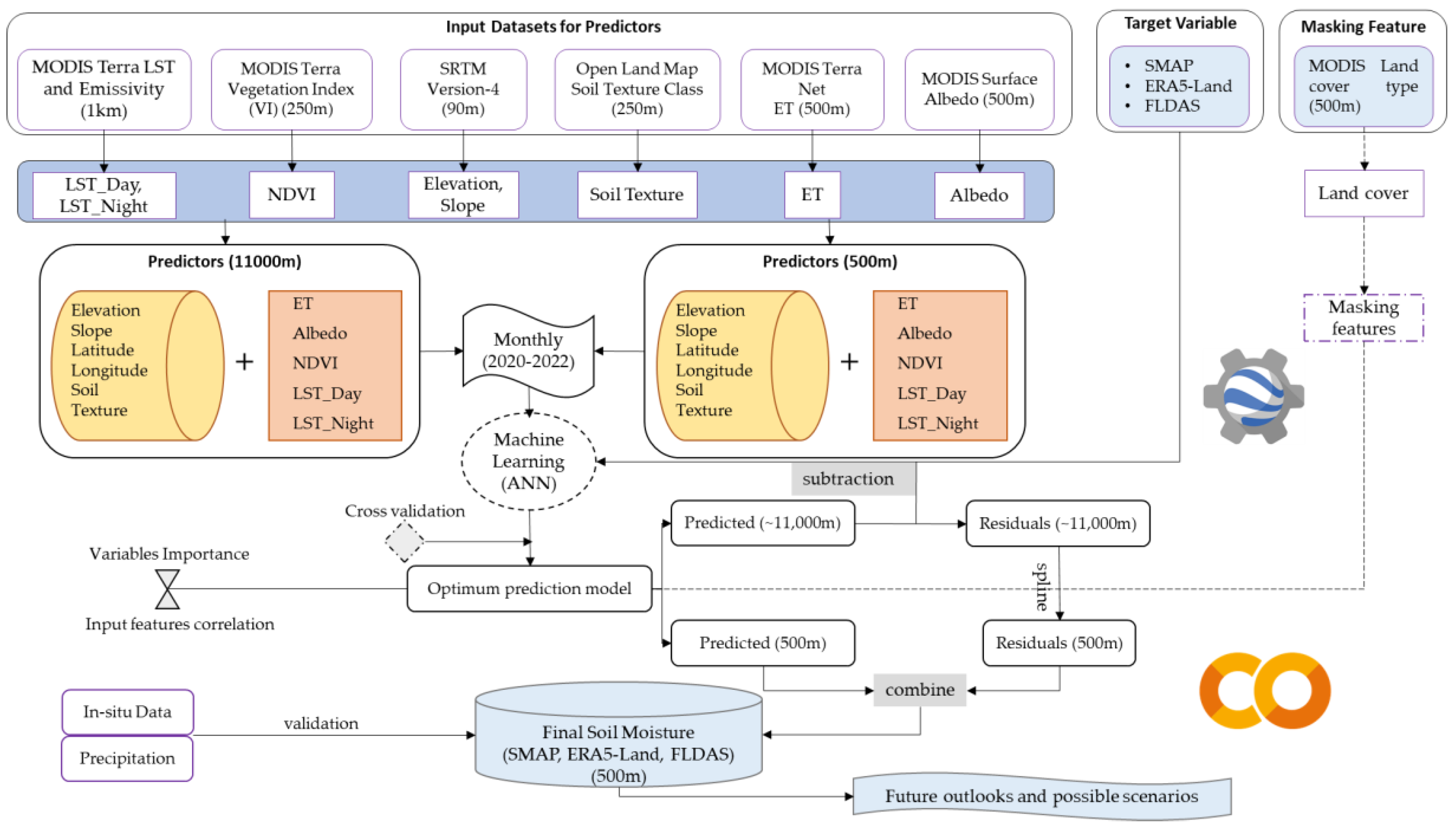
2.4. Proposed Downscaling Framework

Advances in machine learning, along with improved computational facilities and the availability of high-quality datasets, are rapidly advancing the ability to downscale SM. This helps bridge the gap between large-scale environmental monitoring and local-scale water resource management needs [36,64]. In this study, we used an ANN ML algorithm due to its ability to effectively handle noisy data, common characteristics in RS data, and its efficiency in capturing complex relationships between input variables [3,27,28]. The ANN model is designed to create complex connections between various input variables, facilitated by a network of processing units referred to as neurons/nodes [65]. The model consists of an input layer, one or more hidden layers, and an output layer, forming a robust architecture that has been successfully applied in previous studies for downscaling and inverting SM data [25,29].

For this study, a thorough sensitivity analysis of input variables was conducted, and the ten most important predictors were selected: elevation, slope, longitude, latitude, soil texture, ET, albedo, NDVI, LST_Day, and LST_Night. These variables serve as predictors to downscale surface SM in the proposed study region. The anticipated predicate data, including SMAP L4, ERA5-Land, and FLDAS, are chosen to invert high-resolution SM from them by taking advantage of their unique dataset characteristics. According to [27,66], the number of nodes in each hidden layer is determined by multiplying the number of predictors by 2 and adding 1 (number of predictors × 2 + 1), which resulted in 21 nodes in each hidden layer, as presented Figure 2 which is adopted from https://alexlenail.me/ (accessed on 12 September 2024).

The process of downscaling can be mathematically described by SM = F (Yi) + ε, where SM represents the downscaled SM, Yi represents input variables, and ε is the residual. Leveraging the advantage of the ANN model in managing non-relationship data and addressing the noisy data and its capability to manage large datasets, this approach aims to establish a correlation function between output and input variables at a coarse resolution of approximately 11,000 m. This correlation function links input variables to output covariates using the following equations.

$${SM}_{\left(\mathrm{11,000}m\right)}={f\left(predictors\right)}_{\left(\mathrm{11,000} \mathrm{m}\right)}$$

(4)

$${SM}_{\left(500m\right)}={f\left(predictors\right)}_{\left(500 \mathrm{m}\right)}$$

(5)

This implies that the statistical relation obtained from SM and input variables at 11,000 m resolution can be sequentially applied to a 500 m scale. Based on the principles of statistical downscaling, the innovative downscaling framework for this study, presented in Figure 3, is designed, which shows the potential-use datasets from GEE and integrates ANN ML algorithms using Google Colab. The proposed algorithm is used to determine the relationship between the predictors and the anticipated output variables. Cross-validation was adopted to select the most effective ANN hyper-parameters. Furthermore, the downscaling framework follows the principle that the resolution of input variables shall be equivalent to or finer than the predicted output, in order to reduce the uncertainties occurring due to scale mismatching and applying interpolation techniques for multiple datasets.

2.4.1. Data Processing

It is important to note that the quantity of input variables, the geographic extent, and the quantity and spatial resolution of these inputs, can have a direct impact on the temporal resolution and quality of the predicted output [67,68]. In this study, land cover features such as urban built-up areas and permanent water bodies identified in the MODIS land cover data are masked out prior to extracting SM-related features to minimize their influence on the downscaling process used for SM retrieval. The quality control check mechanism and defining a common coordinate system for input datasets (EPSG: 4326) were performed to exclude products and pixels that contained erroneous data, which could have been affected by clouds or aerosols [69].

Furthermore, we utilized an interpolation technique and arithmetic mean methods to address the discrepancies in spatial resolution between the predictors and the target variable. In this case, the coarse resolution predictors were resampled into high-resolution data using bilinear interpolation, while the high-resolution predictors were transformed into a coarse resolution using the basic arithmetic mean. Moreover, the standard scaler algorithm was utilized to standardize the input datasets by considering their mean and standard deviation [70]. In this study, the ten input variables used comprised five static geophysical variables (elevation, slope, latitude, longitude, and soil texture) to depict spatial distribution patterns and the variation in downscaled SM, as well as five dynamic land surface variables (ET, albedo, NDVI, LST_Day, and LST_Night).

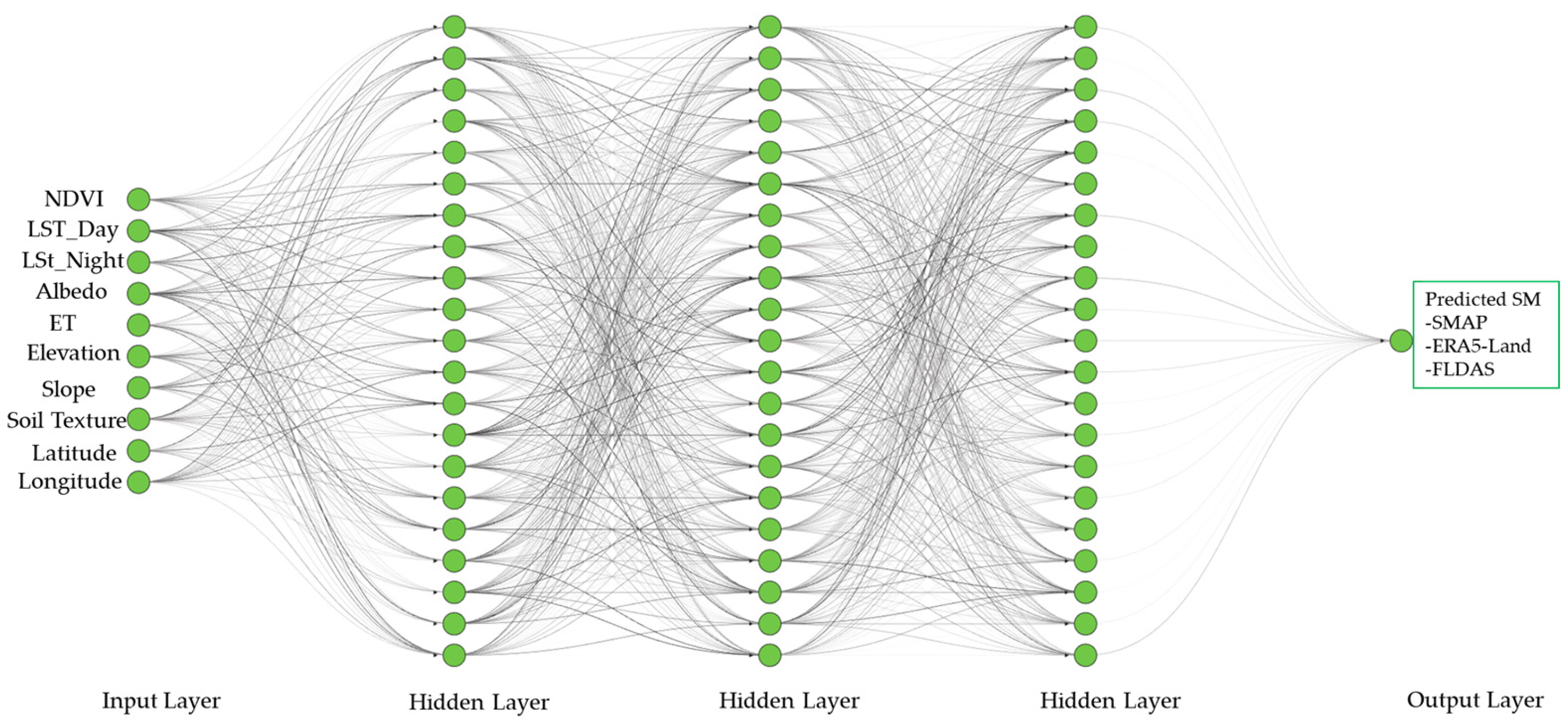
2.4.2. Generating High-Resolution Soil Moisture Data

We highlighted that the proposed study employs an ANN-based ML algorithm to produce SM data with a spatial resolution of 500 m after analyzing the uncertainty among SM products, a task which has not yet been attempted in this region. In order to achieve this objective, the scikit-learn GridSearchCV (GSCV) algorithm with the cross-validation splitting approach was used to determine the optimal hyper-parameter values of ANN for the predicted SM datasets. The total number of pixels at a coarse resolution of 11,000 m was partitioned, allocating 70% for training and testing the algorithms, to define the best hyper-parameters. To do so, we utilized the 10-fold cross-validation (CV = 10) technique to determine the best hyper-parameter for developing the optimum prediction model (OPM). Meanwhile, the remaining 30% pixels were allocated for the purpose of validating the OPM ability to simulate the target variables for the ANN model.

The following major steps were conducted in order to produce high-resolution SM data. First, the input variables were resampled to 11,000 m spatial resolution. The framework considers the dynamic spatiotemporal variability in SM, vegetation, surface temperature, surface albedo, and ET. To maintain consistency in temporal resolution, the dynamic land surface variables were standardized to a monthly scale, while geophysical variables such as soil texture, elevation, and slope, which are constant variables, were considered static. Second, the best-fitting OPM was applied to predict the SM at 11,000 m from input variables at the same resolution. A regression relationship between SM and input variables was established using ANN models for the given period on a monthly basis, and the model accuracy was computed. Third, residual SM was generated at the coarse resolution, where ΔResidual = Original SM − Predicted SM.

Furthermore, the spline algorithm [71] was then used to resample the residual SM from 11,000 m to 500 m, as this method has been shown to perform well for regularly spaced grid datasets [72,73]. Subsequently, the trained model utilized in step 2 was employed to predict SM values at 500 m from input variables with a spatial resolution of 500 m. Finally, the high-resolution SM was obtained following residual correction. It was derived by summing the predicted SM at 500 m to the residual 500 m (Final_SM_500m = Predicted SM_500m + ΔResidual_500m). Each of these steps is implemented individually for the SMAP, ERA5-Land, and FLDAS datasets, respectively.

2.5. Soil Moisture Depth Harmonization

Discrepancies in measurement depths among SM datasets (e.g., SMAP at 0–5 cm, and ERA5-Land at 0–7 cm, and in situ observations (10 cm)) introduce depth-dependent biases during comparative analysis [3,8,52]. To harmonize these datasets, we implemented a depth normalization procedure using an exponential decay function [74,75]. This function assumes that SM decreases exponentially with depth, governed by soil hydraulic properties. The normalized SM at the target depth (10 cm) is as follows:

$${SM}_{normalized}={SM}_{product}{e}^{-\lambda .d}$$

(6)

where ${SM}_{normalized}$ is the depth-adjusted SM at 10 cm, ${SM}_{product}$ is the input SM at the native depth (5 cm for SMAP and 7 cm for ERA5-Land), $d$ is the depth difference between the target (10 cm) and product layers, and $\lambda$ is the decay constant describing SM attenuation with depth.

The decay constant λ is derived from the Mualem–van Genuchten (MvG) model parameters α (inverse air-entry pressure, m⁻¹), which defines the suction head at which soil pores begin to drain, and n (pore-size distribution index), which controls the curvature of the water retention curve [75,76]. Due to the absence of coincident experimental data, λ is derived indirectly using soil hydraulic properties, with values for each in situ station extracted from datasets available at https://gee-community-catalog.org/projects/hihydro_soil/ (accessed on 5 January 2025) to carry out the SM depth normalization [59]. For this study, the normalization procedure was applied to the SMAP and ERA5-Land datasets to standardize the SM values to a consistent 10 cm depth.

2.6. Evaluation Metrics

The downscaled results from the model are assessed and evaluated. Initially, the model precision evaluation was conducted in order to determine the optimum performance of the algorithm considering the relationship and dependency of input variables for the model. In succession, the correlation between the coarse resolution SM and final predicted SM was determined for the chosen period, where the correspondent in situ data was fully available. Finally, the observed in situ data were evaluated against the original SM and the final predicted SM, respectively. For evaluation and visualization purposes, we have selected monthly data from 2020 to 2022 because of limited in situ data availability. In this case, a comprehensive statistical evaluation of the ML performance model was conducted, which mainly comprised the following:

$$r={\displaystyle \frac{{\sum }_{i=1}^n\left(S_i-\overline{S}\right)\left({\widehat{S}}_i-\overline{\widehat{S}}\right)}{\sqrt{\sum _{i=1}^n{\left(S_i-\overline{S}\right)}^2\sum _{i=1}^n{\left({\widehat{S}}_i-\overline{\widehat{S}}\right)}^2}}}$$

(7)

$$UbRMSE=\sqrt{{\displaystyle \frac{1}{n}}\sum _{i=1}^n{[(S_i-\overline{S})-({\widehat{S}}_i-\overline{\widehat{S}})]}^2}$$

(8)

$$MAE={\displaystyle \frac{\sum _{i=1}^n\left|S_i-{\widehat{S}}_i\right|}{n}}$$

(9)

$$KGE=1-\sqrt{{\left(r-1\right)}^2+{\left(\alpha -1\right)}^2+{\left(\beta -1\right)}^2}$$

(10)

where r is the Pearson correlation coefficient between the original and predicted SM, UbRMSE is an unbiased root mean square error, MAE is the mean absolute error, KGE is the Kling–Gupta Efficiency, ${\mathrm{S}}_{\mathrm{i}}$ the original soil moisture, $\widehat{{\mathrm{S}}_{\mathrm{i}}}$ is the predicted soil moisture, $\overline{\mathrm{S}}$ is the mean of the original soil moisture value, $\overline{\widehat{\mathrm{S}}}$ is the mean of the predicted soil moisture, r is the Pearson correlation coefficient between the original and predicted soil moisture, $\mathsf{\alpha }$ is the ratio of the standard deviation of predicted values to the standard deviation of original soil moisture, and $\mathsf{\beta }$ is the ratio of the mean predicted values to the mean of the original soil moisture values. NB: The in situ soil moisture can replace either the original SM or predicted SM for validation purposes.

The Pearson correlation (r) is utilized to quantify the magnitude and direction of the linear relationship between observed and predicted values, or the original and in situ SM data. MAE is employed as a bias indicator, while UbRMSE is used to describe the accuracy of the ML algorithm. Furthermore, KGE is specifically employed to assess the efficiency of the model prediction. Finally, the in situ data collected from the TAHMO networks was used to verify the accuracy of the final downscaled results using r, UbRMSE, and MAE.

3. Results

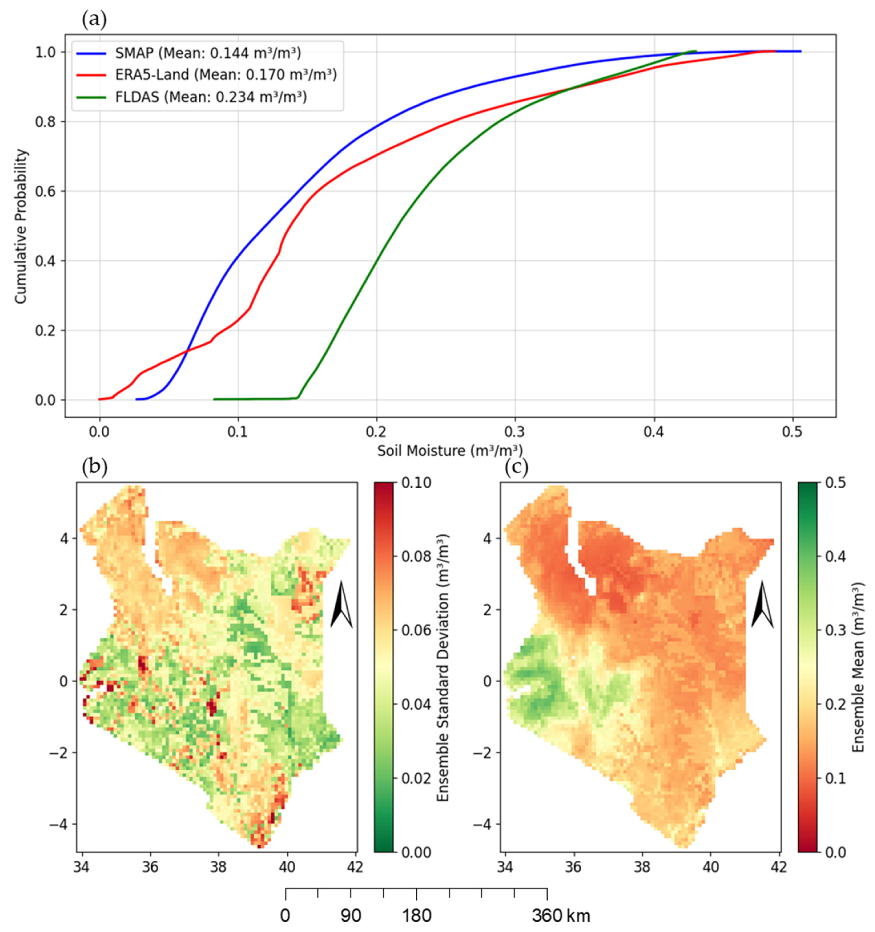
3.1. Uncertainty Analysis of Multi-Source Soil Moisture Products

Figure 4 presents the cumulative distribution function (CDF), ensemble standard deviation (ESD), and ensemble mean (EM) of SM derived from the original SMAP, ERA5-Land, and FLDAS datasets over the period 2020–2022. The CDF analysis (Figure 4a) reveals that SMAP and ERA5-Land exhibit relatively closer agreement in terms of SM distribution compared to FLDAS, which shows systematically higher values. The mean SM values of 0.144 m³/m³ for SMAP and 0.170 m³/m³ for ERA5-Land suggest a moderate alignment, whereas FLDAS shows a notable deviation with a mean of 0.234 m³/m³. Relatively, FLDAS demonstrates the narrowest range of SM values (0.083–0.430 m³/m³), followed by SMAP (0.027–0.506 m³/m³) and ERA5-Land (0.001–0.487 m³/m³). The ESD map (Figure 4b) further reveals that the variability among the datasets is below 0.015 m³/m³ across the domain. This indicates strong agreement and consistency among the datasets, with an average ESD of 0.024 m³/m³, aligning well with the threshold of acceptable variability outlined by [77].

The ensemble mean map (Figure 4c) identifies distinct spatial patterns in SM distribution, with higher SM values observed in western regions, potentially reflecting wetter climatic or hydrological conditions. Conversely, lower SM values are prominent in the northern and northeastern regions, indicative of drier conditions. This result provides critical insight into downscaling SM products to higher spatial resolutions, emphasizing the importance of leveraging the strengths of consistent datasets to ensure robust and accurate downscaled products.

3.2. Optimum Prediction Model of the Proposed Downscaling Framework

To evaluate the prediction accuracy and examine the characteristics of the original coarse-scale SM products, we computed the monthly performance metrics over a three-year period (2020–2022). These metrics include r, UbRMSE, MAE, and KGE for SMAP, ERA5-Land, and FLDAS, respectively. As illustrated in Figure 5a, the correlation coefficient (r) indicates a strong agreement between the coarse-resolution and downscaled SM products across all datasets. The mean r values for SMAP, ERA5-Land, and FLDAS are 0.88, 0.92, and 0.96, respectively, with FLDAS consistently achieving the highest correlation among all datasets. The error metrics further reinforce the superior performance of FLDAS. In Figure 5b, the UbRMSE values indicate that FLDAS achieves the lowest mean error (0.016 m³/m³) compared to SMAP (0.038 m³/m³) and ERA5-Land (0.040 m³/m³). A similar pattern is observed for MAE (Figure 5c), where FLDAS maintains the lowest mean error with a MAE value of 0.011 m³/m³, followed by SMAP and ERA5-Land, with values of 0.028 m³/m³ and 0.029 m³/m³, respectively. The KGE, shown in Figure 5d, further demonstrates an overall agreement of the downscaled products with the coarse-resolution counterparts. FLDAS achieves the highest mean KGE of 0.95, surpassing ERA5-Land (0.90) and SMAP (0.85).

On a monthly basis (

Table 3. Monthly prediction/test accuracy of downscaled SM for SMAP, ERA5-Land, and FLDAS.

Month	r			KGE			UbRMSE (m3/m3)			MAE (m3/m3)
	SMAP	ERA5-Land	FLDAS	SMAP	ERA5-Land	FLDAS	SMAP	ERA5-Land	FLDAS	SMAP	ERA5-Land	FLDAS
January	0.89	0.92	0.96	0.86	0.91	0.94	0.039	0.040	0.016	0.029	0.029	0.011
February	0.91	0.94	0.98	0.89	0.92	0.97	0.039	0.041	0.013	0.028	0.029	0.009
March	0.89	0.91	0.97	0.87	0.88	0.95	0.037	0.040	0.014	0.026	0.028	0.010
April	0.87	0.91	0.92	0.84	0.89	0.90	0.038	0.041	0.017	0.028	0.030	0.012
May	0.88	0.92	0.94	0.85	0.90	0.92	0.043	0.041	0.020	0.032	0.030	0.014
June	0.85	0.91	0.96	0.82	0.87	0.95	0.043	0.040	0.018	0.032	0.029	0.012
July	0.85	0.91	0.96	0.82	0.89	0.95	0.040	0.039	0.017	0.030	0.028	0.011
August	0.89	0.93	0.97	0.86	0.91	0.96	0.037	0.039	0.015	0.028	0.027	0.010
September	0.90	0.93	0.98	0.87	0.91	0.98	0.036	0.038	0.014	0.027	0.027	0.009
October	0.89	0.91	0.97	0.86	0.89	0.96	0.035	0.040	0.015	0.026	0.028	0.011
November	0.87	0.90	0.94	0.84	0.87	0.92	0.035	0.041	0.017	0.026	0.030	0.013
December	0.88	0.92	0.95	0.85	0.89	0.94	0.038	0.043	0.017	0.027	0.031	0.012

Note: The bold values indicate the highest accuracy of the product within each month.

), February stands out as the month where all datasets exhibited the highest prediction accuracy, especially in terms of correlation and efficiency value. FLDAS achieved a remarkable monthly mean correlation value of 0.98 in February, followed by ERA5-Land and SMAP, with correlation coefficient values of 0.94 and 0.91, respectively. On the contrary, the lowest correlation values for SMAP and ERA5-Land occurred in June and November, respectively, while FLDAS showed its lowest correlation in April, although it still maintained relatively high performance. In terms of predicting the coarse resolution SM data, FLDAS is a more reliable SM product, making it the most effective dataset for capturing the monthly variability and bridging the gap between coarse-resolution and downscaled products.

3.3. Roles of Input Variables to Downscale Multi-Source SM Datasets

An analysis of the input features’ correlation and an assessment of the features’ relative importance provide a thorough understanding of how various environmental and climatic variables contribute to downscale SM from multi-source datasets. Figure 6a–c reveal consistent patterns of correlation between the input variables and SM datasets, highlighting both shared and dataset-specific sensitivities. From the land surface dynamic input variables, LST_Day and LST_Night exhibit moderate to strong negative correlations across all three datasets, indicating their significant role in reducing SM, likely due to their impact on evaporation and the surface drying process [78]. The variability in LST pattern is mostly pronounced in FLDAS (Figure 6c), with a slightly weaker correlation observed in SMAP (Figure 6a) among other datasets.

In contrast, NDVI and ET demonstrate strong positive correlations, underscoring their importance in maintaining SM [1]. The relationship is relatively consistent across the datasets, with FLDAS showing slightly stronger correlations for NDVI and ET compared to SMAP and ERA5-Land. Additionally, albedo exhibits weak to moderate negative correlations with SM, typically ranging from −0.4 to 0. This indicates that a higher albedo, often associated with drier soils and reduced absorption of solar radiation, is inversely related to SM. However, the correlation remains relatively weak due to other influencing factors, such as vegetation factor and soil composition, which can dilute the direct relationship between albedo and SM [55]. These findings emphasize the critical roles of temperature, vegetation, water fluxes, and surface reflectivity in SM variability.

From the topographic parameters, elevation exhibits a moderate positive correlation across the datasets, reflecting its influence on SM, potentially through cooler temperatures and reduced evaporation at higher altitudes. In contrast, slope demonstrates poor correlations, indicating minimal direct influence on SM across the datasets [50]. Soil texture, on the other hand, consistently shows a moderate negative correlations, highlighting its role in water retention, where finer textures are often associated with lower available water [52]. Additionally, latitude and longitude display moderate correlations, with some variability depending on the dataset. Overall, these findings reveal consistent yet nuanced sensitivities of each SM product to environmental drivers, emphasizing the importance of these variables in refining downscaling approaches tailored to specific datasets.

The feature importance analysis was conducted using the permutation importance algorithm from the scikit-learn package version 1.6.1 [79]. As presented in Figure 7, longitude and latitude were identified as the most influential variables across all datasets, with FLDAS showing a higher reliance on these spatial features. Elevation, LST_Night, and LST_Day were found to have moderate importance, with temperature-related variables playing a slightly more significant role in the SMAP and ERA5-Land datasets. Vegetation- and water-related variables, such as ET and NDVI, consistently contributed at moderate levels, with ERA5-land attributing slightly higher importance (over 10%) to ET, followed by FLDAS, emphasizing its role in water flux dynamics. In contrast, variables such as albedo, slope, and soil texture showed minimal importance across all datasets. It is important to note that the feature importance rankings derived from the ANN model represent the average contributions of each variable during the prediction of the target variable in the training process. However, these rankings do not directly indicate the ability of each variable to provide spatial details. Overall, these findings indicate that the contributions of each input variable to downscale SM would fluctuate depending on the dataset, geographic region, and time periods considered.

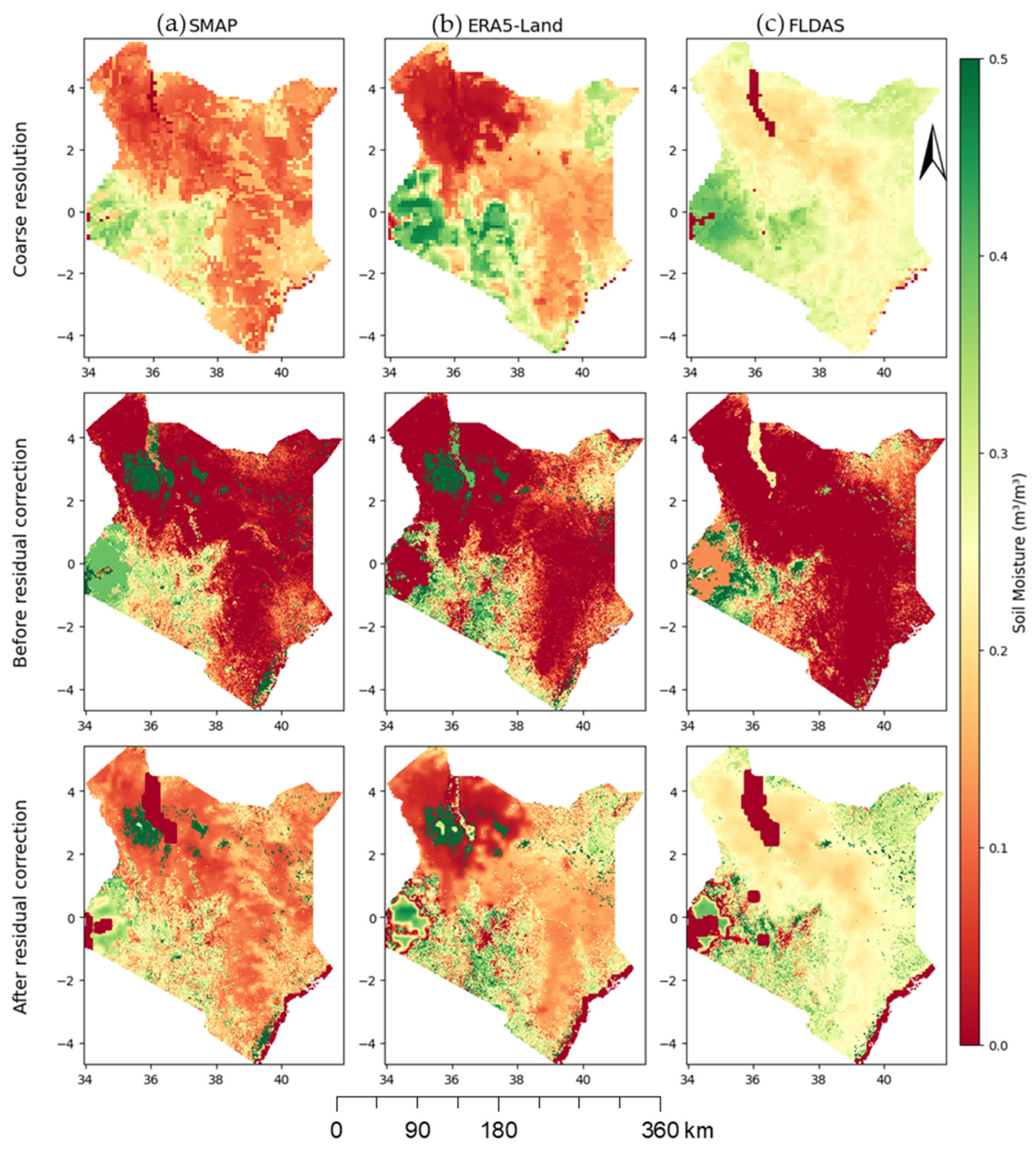
3.4. Spatial Distribution of Multi-Source SM Products

To visually analyze and compare the spatial distribution of SM, SM maps from each dataset before and after downscaling were generated and are shown in Figure 8 and Figure 9, representing the dry and wet periods of February and April 2021, respectively. Residual correction was performed as a critical step to generate the final high-resolution SM maps. Notably, certain pixels do not have SM values observed in either the original or downscaled datasets. This issue arises due to two main reasons: (1) the original datasets often exclude pixels over areas such as major water bodies, and (2) pixels corresponding to land use types unsuitable for SM prediction (i.e., urban/built up areas and water bodies) are omitted from the analysis. Residual correction ensures that discrepancies are minimized, thereby improving the spatial detail and consistency of the final downscaled SM data.

The coarse resolution SM datasets presented in Figure 8a–c and Figure 9a–c derived from SMAP, ERA5-Land, and FLDAS exhibit similar spatial trends and distribution of SM, although differences in magnitude are evident. Variations are particularly noticeable in areas such as water bodies, which are initially masked out in some of the datasets (i.e., FLDAS), as seen in the northern and western regions of Kenya, where water bodies are prominent.

The datasets presenting the downscaled SM before the residual is corrected (BC) (second row) in Figure 8 and Figure 9 exhibits a relative spatial consistency with the coarse resolution datasets, although there are notable variations and uncertainties in magnitude of each dataset. Besides this, the process of excluding areas with specific land use types from estimating SM was not identified, which was later accomplished by correcting the residuals.

The downscaled SM datasets after residual correction (AC) shown in Figure 8a–c and Figure 9a–c display spatial distributions and magnitudes that closely align with the original coarse-resolution SM data, while simultaneously improving the spatial detail. Residual correction effectively enhances spatial consistency, ensuring the downscaled data are more accurate and suitable for interpretation. Among the datasets, FLDAS (Figure 8c and Figure 9c) consistently exhibit relatively higher SM values compared to SMAP and ERA5-Land in most parts of the county, especially in arid and semi-arid regions. In terms of spatial SM distribution, the highest SM concentrations are observed in the western regions of Kenya, particularly in agricultural zones and wetlands near the lakes during dry (Figure 8) and wet (Figure 9) periods. Temporally, this trend is more pronounced during the wet period (Figure 9).

Conversely, the northern and northeastern regions, characterized by arid and semi-arid landscapes dominated by grasslands and shrublands, have the lowest SM values. This indicates that the downscaling can improve the spatial detail, and residual correction ensures consistency across the datasets, particularly for regions with variable climate conditions and land cover.

3.5. Visualizing the Temporal Patterns of Downscaled Products

Several studies have suggested that SM has a predominantly positive influence on precipitation [24,80]. In this study, we analyzed the temporal patterns of both the original and downscaled datasets at station locations where in situ data are available. Additionally, we utilized monthly precipitation data retrieved from Climate Hazards Center Infrared Precipitation with Station data [81] to examine the SM patterns along with precipitation. Figure 10a–k demonstrates that both the original and downscaled datasets generally exhibit trends consistent with the trends observed in the in situ data, albeit with varying magnitudes. This indicates the importance of leveraging multiple datasets to achieve a comprehensive understanding of SM dynamics. The SM levels tend to fluctuate throughout the year, with noticeable increases corresponding to months with higher precipitation, particularly in April and November. Among the datasets analyzed, FLDAS and its downscaled counterpart show consistently higher SM values, as illustrated in Figure 10a,b,d–f,j,k. This suggests that FLDAS tends to predict an elevated SM level across most stations when compared to SMAP and ERA5-Land.

Notably, the downscaled SM datasets tend to show a closer relationship with the in situ SM observations and monthly precipitation patterns compared to their original counterparts. This indicates that the downscaling process enhances the datasets’ sensitivity to precipitation changes by improving spatial resolution, which allows for the capture of a more localized variation in SM driven by precipitation. Overall, the SM datasets demonstrate strong responses to precipitation events, showing an increasing trend during or shortly after precipitation occurs.

3.6. Verification of Multi-Source Downscaled SM Data

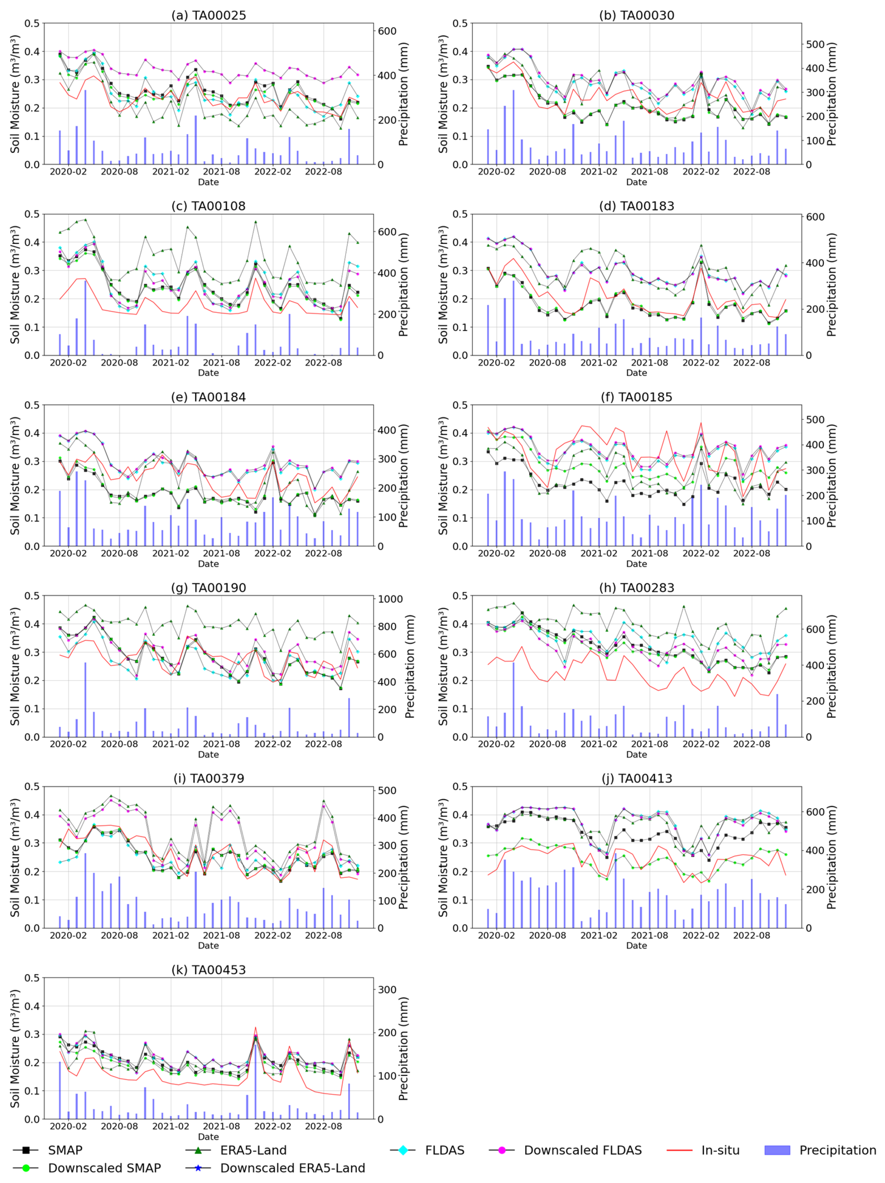
3.6.1. Station-Based Validation

To validate the performance of the proposed method, we used in situ data as a reference for comparison with the coarse-resolution SM and their corresponding downscaled versions. This validation was carried out for the stations located in Kenya over the period from 2020 to 2022. Figure 11 showcases the scatter plots that illustrate the overall performance of the proposed SM datasets and their downscaled counterparts against the in situ SM data. These plots provide a visual representation of the relationship and agreement between the datasets. Additionally,

Table 4. Correlation coefficient (r) between in situ SM and estimated SM datasets at different stations.

Station	SMAP	ERA5-Land	FLDAS	Downscaled SMAP	Downscaled ERA5-Land	Downscaled FLDAS
TA00025	0.80	0.73	0.78	0.77	0.75	0.81
TA00030	0.83	0.85	0.83	0.82	0.85	0.84
TA00108	0.84	0.87	0.82	0.83	0.87	0.83
TA00183	0.91	0.77	0.84	0.91	0.79	0.84
TA00184	0.74	0.84	0.71	0.73	0.83	0.73
TA00185	0.58	0.76	0.58	0.52	0.79	0.58
TA00190	0.66	0.75	0.66	0.65	0.77	0.64
TA00283	0.70	0.77	0.74	0.66	0.76	0.75
TA00379	0.88	0.84	0.78	0.88	0.84	0.79
TA00413	0.67	0.72	0.77	0.69	0.71	0.78
TA00453	0.81	0.79	0.77	0.84	0.81	0.78
Average	0.77	0.79	0.75	0.75	0.80	0.76

Note: The bold values indicate better performing datasets at each station. The correlation values are determined at p < 0.01.

,

Table 5. Unbiased root mean square error (UbRMSE) between in situ SM and estimated SM datasets at different stations.

Station	SMAP	ERA5-Land	FLDAS	Downscaled SMAP	Downscaled ERA5-Land	Downscaled FLDAS
TA00025	0.046	0.056	0.038	0.039	0.042	0.023
TA00030	0.045	0.042	0.030	0.044	0.042	0.029
TA00108	0.036	0.047	0.048	0.036	0.043	0.041
TA00183	0.024	0.043	0.032	0.024	0.051	0.032
TA00184	0.035	0.049	0.038	0.036	0.046	0.037
TA00185	0.059	0.048	0.058	0.063	0.044	0.059
TA00190	0.048	0.029	0.042	0.047	0.028	0.043
TA00283	0.042	0.034	0.033	0.042	0.035	0.033
TA00379	0.031	0.045	0.041	0.031	0.046	0.040
TA00413	0.034	0.029	0.033	0.031	0.030	0.033
TA00453	0.032	0.032	0.034	0.030	0.032	0.034
Average	0.039	0.041	0.039	0.038	0.040	0.037

Note: The bold values indicate better performing datasets at each station.

and

Table 6. MAE between in situ SM and estimated SM datasets at different stations.

Station	SMAP	ERA5-Land	FLDAS	Downscaled SMAP	Downscaled ERA5-Land	Downscaled FLDAS
TA00025	0.034	0.049	0.032	0.029	0.031	0.101
TA00030	0.038	0.036	0.052	0.037	0.036	0.059
TA00108	0.067	0.163	0.079	0.061	0.150	0.071
TA00183	0.027	0.091	0.095	0.025	0.060	0.094
TA00184	0.055	0.040	0.056	0.053	0.037	0.059
TA00185	0.106	0.070	0.050	0.062	0.037	0.051
TA00190	0.039	0.123	0.034	0.039	0.116	0.043
TA00283	0.098	0.177	0.123	0.090	0.159	0.096
TA00379	0.028	0.079	0.035	0.028	0.029	0.033
TA00413	0.095	0.124	0.131	0.025	0.126	0.128
TA00453	0.058	0.046	0.067	0.046	0.024	0.068
Average	0.059	0.091	0.069	0.045	0.073	0.073

Note: The bold values indicate better performing datasets at each station.

present detailed performance metrics for each station, including statistical measures such as r, UbRMSE, and MAE. The analysis was conducted on a monthly scale, considering only the stations where both in situ and SM products are available.

The correlation coefficient (r), as summarized in Table 4, indicates that the downscaled SM datasets generally exhibit moderate to high agreement with in situ SM data. The highest correlation was observed at station TA00183, where the downscaled SMAP achieved an r value of 0.91, showcasing excellent alignment with the in situ data. Conversely, the lowest correlation was observed at station TA00185, where the downscaled SMAP attained an r value of 0.52. While the downscaled products generally perform comparably to their non-downscaled counterparts, minor improvements are evident at most stations.

As presented in Table 5, the UbRMSE values reveal moderate variability in performance across different stations. The lowest UbRMSE was recorded for the downscaled FLDAS at station TA00025, with a value of 0.023 m³/m³, indicating high accuracy. Among the datasets, ERA5-Land and its downscaled version consistently exhibited lower variability in UbRMSE values across stations, followed by FLDAS and its counterparts. However, SMAP and its downscaled versions showed the highest variability in performance.

The MAE comparison, as shown in Table 6, illustrates how the downscaling process influences the alignment of SM datasets with the in situ observations. For the SMAP and ERA5-Land dataset, downscaling tends to reduce MAE values in most cases, indicating an improved consistency with the in situ data. However, in the case of FLDAS, the impact of downscaling is more variable. While the downscaled MAE values improved at some stations, such as TA00283 from 0.123 m³/m³ to 0.096 m³/m³, there are cases where the error slightly increased or remained close to the original, such as at station TA00030 from 0.052 m³/m³ to 0.059 m³/m³.

In general, the downscaled SM datasets show improved or maintained consistency with the in situ observations in most stations, highlighting the effectiveness of the proposed downscaling method. However, the variability in performance among different datasets and stations underscores the influence of localized climate conditions, environmental factors, and the inherent characteristics of each dataset on the downscaling process.

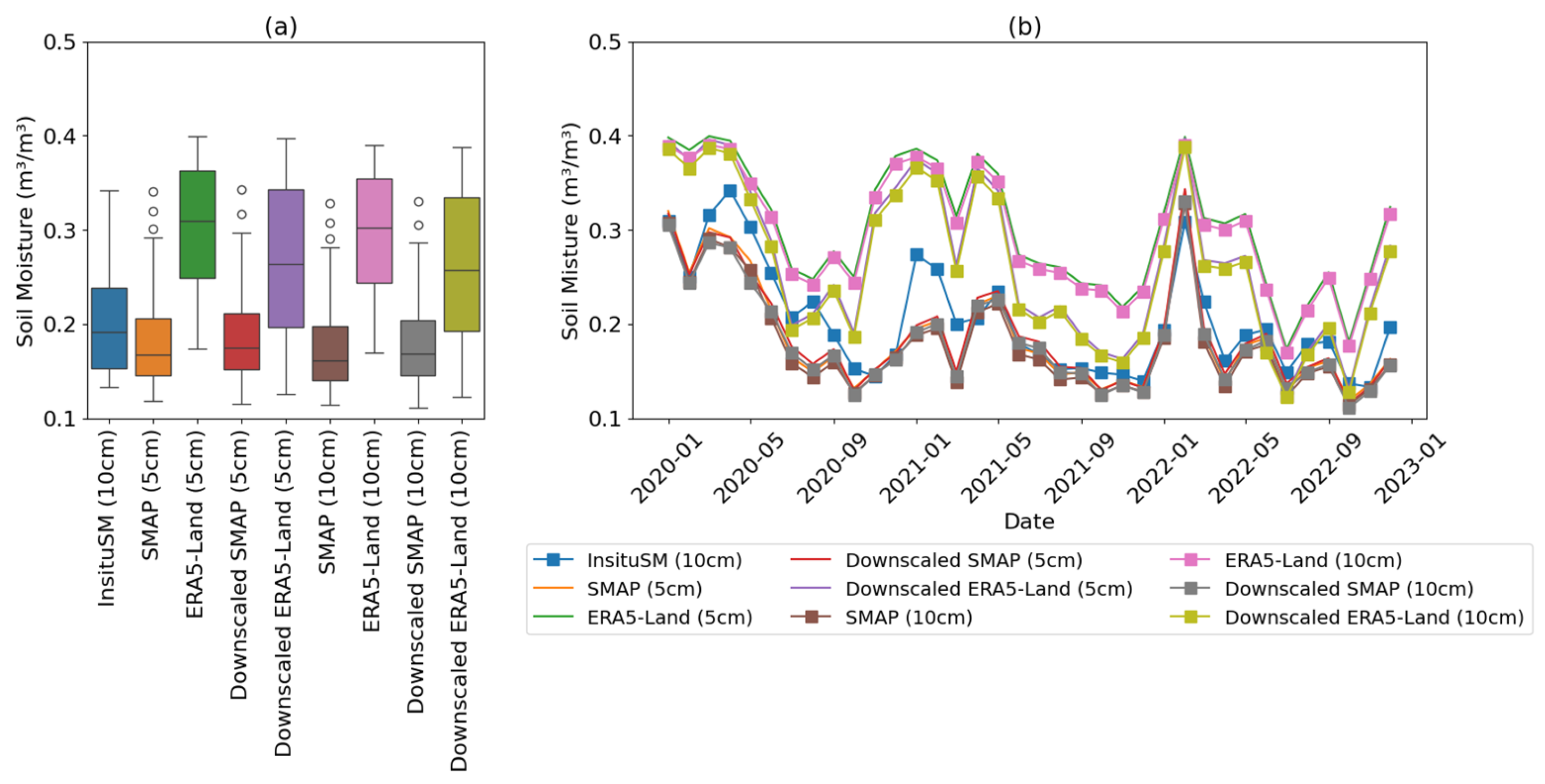
3.6.2. Overall Validation

Furthermore, the overall performance assessment of the original and downscaled SM products against the in situ data is presented in Figure 11. The results demonstrate that the downscaled datasets consistently outperform their coarse-resolution counterparts in capturing local SM conditions. For instance, the original coarse-resolution SMAP data (Figure 11a) exhibit a modest correlation with in situ SM, achieving an r value of 0.48 and an UbRMSE of 0.072 m³/m³. However, after applying the downscaling process, the performance improves significantly, with the r value increasing to 0.64 and the UbRMSE decreasing to 0.057 m³/m³. Similarly, the performance of ERA5-Land (Figure 11d) shows notable improvements following the downscaling, with the r value increasing from 0.47 to 0.63 and the UbRMSE decreasing from 0.087 m³/m³ to 0.075 m³/m³.

Among all datasets, the downscaled FLDAS (Figure 11f) demonstrates better performance, achieving the lowest UbRMSE of 0.052 m³/m³ and the highest r value of 0.69. These results emphasize the effectiveness of the downscaling process in enhancing the agreement between satellite-derived SM datasets and in situ measurements. Overall, the validated SM products demonstrate accuracy levels consistent with those in previous studies on SM variability. For example, the UbRMSE result in this study lies in a agreement with the findings from prior studies [2,9], revealing a SM value range from 0.04 to 0.13 m³/m³. In this study, UbRMSEs below 0.060 m³/m³ have been achieved across most stations. These results highlight the downscaling approach’s ability to enhance or maintain the spatial accuracy and representation of SM conditions, bringing them closer to in situ observations and ensuring better reliability for local-scale applications regardless of varying magnitudes of multi-source SM products.

3.6.3. Validation Across Varying Climate Zones

As shown in Figure 12, FLDAS and its downscaled version demonstrate superior accuracy in the tropical savannah and temperate no dry season climate zones by exhibiting r > 0.59. In contrast, ERA5-Land performs poorly in both of these zones (r < 0.4), while SMAP exhibits low performance in the tropical savannah zone (Figure 12a). However, SMAP and its downscaled version yield better results in the arid steppe hot zone, achieving r values of 0.81 and 0.84, respectively. In terms of UbRMSE, the lowest value (0.029 m³/m³) was exhibited by ERA5-Land in the tropical monsoon climate zone (Figure 12c). In the temperate dry warm and summer warm, all datasets show improved performance, with SMAP leading in terms of accuracy. Notably, FLDAS and its downscaled variant has shown consistent results, among others, across the various climate zones. Across all climate zones, the downscaled products consistently outperform their original versions, indicating that their finer resolution enhances accuracy.

4. Discussion

4.1. Significance of Input Variables in Downscaling Multi-Source SM Data

The process of SM variation is complex, which is influenced by intricate interactions among topography, vegetation, soil properties, and climatic conditions, all of which exhibit significant spatial and temporal variability. Downscaling SM to finer resolutions is challenging due to the need for models to effectively capture these dynamics [11,13,16,24]. This study addressed this challenge by incorporating a diverse set of input variables (elevation, slope, NDVI, ET, LST_Day, LST_Night, albedo, soil texture, latitude, and longitude), which are crucial in capturing the spatial heterogeneity of SM as presented in Figure 6 and Figure 7, respectively. Among the input variables, ET, NDVI, LST_Day, and LST_Night have shown strong correlations, highlighting their importance in capturing spatial and temporal variability.

Furthermore, elevation, longitude, latitude, and ET are the most important features shown consistently throughout the months, with other factors showing varying levels of influence depending on the characteristics of dataset. The SM datasets from different sources may be influenced by input variables differently, with varying magnitudes across spatial and temporal scales [11]. However, in this study, the selected SM datasets exhibited a standard deviation below 0.15 m³/m³, indicating their high consistency in representing the SM conditions over varying landscapes.

4.2. Discrepancies in Depth, Spatial, and Temporal Scales of Datasets

A critical step in the downscaling process involved the standardization of input variables to address the discrepancies in the spatial and temporal scales of the datasets and the correction of residuals. Such discrepancies can introduce uncertainties in capturing SM variability [11,14,82,83]. To minimize these uncertainties, the datasets were aggregated on a monthly basis to enable downscaling from coarse resolution (~11,000 m) to a finer resolution (500 m). This approach followed the statistical downscaling method, ensuring that all input variables shall exhibit a spatial resolution of 500 m or finer. However, some challenges persisted. For instance, the MODIS LST data, originally available at 1 km resolution, were interpolated to 500 m using bilinear interpolation. While necessary, this process introduced uncertainties, potentially affecting downscaling accuracy [84].

Moreover, variations in the recording depths of the surface SM among datasets (SMAP: 0–5 cm, ERA5-Land: 0–7 cm, and FLDAS: 0–10 cm) resulted in inconsistencies when compared to the in situ observations [22,83], with only FLDAS recording SM at the same depth as the in situ data. To address these discrepancies, Figure 13 presents the normalized SM values, which were adjusted by an exponential decay constant λ [74,75,76]. These normalized values show a closer alignment with the in situ data, as reflected in the downward trend observed in the trend analysis (Figure 13b).

While there was no significant difference in the r values between the in situ data and both pre- and post-normalized values, improvements were observed in the UbRMSE and MAE after normalization. This indicates that depth variations across datasets likely contributed to the differing validation results against the in situ data. FLDAS, however, demonstrated consistent performance across different climate zones, likely because of its measuring depth (10 cm) and its data characteristics [46,75]. The λ, which is influenced by factors such as soil texture and soil hydraulic conductivity, plays a critical role in improving the accuracy of SM estimation [75]. Incorporating experimental ground data could further refine the accuracy of SM validation, offering more precise adjustments to account for spatial and temporal variations in soil properties.

Furthermore, as presented in Figure 8 and Figure 9, residual correction was implemented during the downscaling of the SM datasets to address errors and inconsistencies that arise from multiple sources throughout the process [3]. It was applied during the transitioning from coarse-resolution datasets to finer resolutions, which often introduces uncertainties due to limitations in the input data, interpolation method, and model assumptions. Apart from these, the inherent variability in SM values across heterogeneous landscapes, such as urban areas and water bodies amplifies these inaccuracies. To mitigate this, this study employed residual correction techniques [3,17] that improved the spatial consistency of the downscaled datasets, aligning them more closely with their original counterparts without sacrificing their accuracy. Figure 14 presents the residual map for coarse resolution and fine resolution, respectively, by taking February in 2021 as an example. The map shows where the model overestimates (red) and underestimates (green) while predicting the coarse resolution before a correction was performed.

4.3. Spatiotemporal Variability Effects of Downscaled Results

The analysis of the coarse and downscaled datasets demonstrates that the proposed downscaling framework effectively enhances the spatial and temporal representation of SM, even in regions with diverse landscapes, such as Kenya. By using multi-source datasets (SMAP, ERA5-Land, and FLDAS), the downscaling process captures spatiotemporal variability across the study area, improving the correlation with in situ measurements despite the variations in SM magnitude. At the station level, the framework consistently improves or maintains the accuracy of the original SM datasets. As shown in Figure 5, the FLDAS dataset achieved the prediction accuracy with the lowest mean UbRMSE of 0.016 m³/m³, while the SMAP predictions resulted in the highest mean UbRMSE of 0.040 m³/m³. Similarly, the correlation with the in situ data improved significantly, with the downscaled FLDAS dataset achieving the lowest UbRMSE of 0.023 m³/m³, while the three datasets achieved an UbRMSE of below 0.060 m³/m³ for each station (Table 5). Across all datasets, the proposed framework consistently improved the correlation (r) values, with increases from 0.48 to 0.64 for SMAP, 0.47 to 0.63 for ERA5-Land, and 0.60 to 0.69 for FLDAS (Figure 11).

These improvements highlight the capability of the downscaling framework to better capture spatiotemporal variability, even in regions with limited validation data. While the distribution and location of validation sites are critical for evaluating SM products [9,85], this study faced challenges due to the sparse availability of in situ measurements across East Africa. This limited number of ground station for a short period of time makes it difficult to fully validate the SM datasets, as these stations may not adequately capture the spatial variability of the region. Nevertheless, the downscaled results demonstrate clear improvements in both spatial resolution and correlation with in situ measurements, despite these challenges. This indicates the robustness of the framework and its potential to serve as a reliable standard and scalable method for downscaling SM data in regions with limited validation resources.

4.4. Comparison with Previous Studies

The accuracy of downscaled SM datasets is influenced by numerous factors, including the choice of downscaling methods and the incorporation of input variables. As summarized in

Table 7. Comparison of the proposed model with related published studies.

Prediction Model	Input Variables	Soil Moisture	Downscaled Resolution	Study Area	Performance (r, UbRMSE (m3/m3))	Source
RF	MODIS (LST, Albedo, NDVI, NDWI, LAI), Elevation	SMAP (36 km)	1 km	CONUS	UbRMSE USCRN: 0.040, SCAN: 0.047	[1]
RT, ANN, GPR	MODIS (LST, NDVI), and soil clay	SMAP (~9 km)	1 km	Australia	UbRMSE RT: 0.07, ANN: 0.08, GPR: 0.05	[20]
Data Fusion, BME	MODIS (EVI, Albedo, LST)	ESA CCI (~25 km)	1 km	Tibetan Plateau	r = 0.592 UbRMSE = 0.083	[16]
CART, KNN, BAYE, RF	MODIS (LST_Day, LST_Night, ΔLST, NDVI, Spectral bands, DEM	ESA CCI (~25 km)	1 km	China	r2 CART: 0.135, KNN: 0.130, BAYE: 0.119, RF: 0.191 RMSE CART: 0.076, KNN: 0.074, BAYE: 0.075, RF: 0.073	[24]
RF	MODIS (LST, ΔLST, NDVI, Reflectance bands)	SMAP L4 (~9 km)	1 km	Ghana & Kenya	Ghana (r = 0.64, UbRMSE = 0.058) Kenya (r = 0.65, UbRMSE = 0.110)	[2]
SVR	MODIS (LST, NDVI)	ASCAT (~12.5 km)	1 km	Korea	r = 0.68 RMSE = 0.07	[14]
Wide and Deep Learning (WDL)	Brightness temperature/s, LST, surface reflectance, soil properties, DEM, land use, precipitation	SMAP SM (SPL3SMP, 36 km)	1 km	CONUS	r = 0.325–0.997, average of 0.715 UbRMSE = 0.010–0.141, average of 0.04	[17]
Bayesian	MODIS (NDVI, LST), Interpolated SMAP	SMAP (~9 km)	1 km	CONUS	r = 0.88, UbRMSE = 0.053	[85]
ANN RF	NDVI, EVI, NDWI, LSWI, NSDSI, LST, elevation, slope, and aspect	SMAP (SPL3SMP, 36 km)	1 km	China	ANN + Terra (r = 0.44, UbRMSE = 0.048) RFR + Terra (r = 0.52, UbRMSE = 0.037) ANN + Aqua (r = 0.51, UbRMSE = 0.051) RFR + Aqua (r = 0.50, UbRMSE = 0.039)	[32]
DISPATCH TRAPEZOID	SEVIRI LST, FVC (43 km)	SMOS (~12.5 km)	5 km	West Africa	RMSE = 0.034–0.11	[86]
ANN	MODIS (NDVI, ET, Albedo, LST_Day, LST_Night), Elevation, Slope, Soil Texture, Latitude, and Longitude	SMAP, ERA5-Land, FLDAS (~9 km)	500 m (0.5 km)	Kenya	r SMAP: 0.52–0.91 ERA5-Land: 0.71–0.87 FLDAS: 0.58–0.84 UbRMSE SMAP: 0.024–0.063 ERA5-Land: 0.028–0.051 FLDAS: 0.023–0.059	This Study

, most downscaling approaches such as physical, regression, and hydrological models primarily rely on linear relationships to link input variables to SM [1,2,16,86]. While these methods have yielded useful results, they often oversimplify the complex, non-linear relationships between SM and input variables, limiting their ability to fully capture the complex dynamics influencing SM patterns. In contrast, ML-based methods, including ANN, leverage non-linear relationships to model SM with greater precision [17,22,32]. However, many ML-based studies rely on a limited set of input variables, often failing to account for critical environmental factors affecting SM [17]. Furthermore, the majority of these studies downscale SM data exclusively from RS products, neglecting the complementary value of reanalysis and land data assimilation products.

To address these limitations, this study developed a cloud-based ANN downscaling framework that integrates both land surface variables (e.g., ET, LST_Day, LST_Night, NDVI, and albedo) and geophysical variables (e.g., soil texture, elevation, slope, latitude, and longitude). This framework generates high-resolution SM datasets (500 m) from three diverse sources: SMAP, ERA-Land, and FLDAS. The ANN model demonstrated exceptional accuracy, achieving mean UbRMSEs of 0.038 m³/m³ for SMAP, 0.040 m³/m³ for ERA5-Land, and 0.037 m³/m³ for FLDAS datasets. These results are comparable to, and in many cases exceed, the accuracy achieved by previous studies and fulfilled the standard accuracy set for SM prediction (see Table 7). The integration of diverse input variables and multiple data sources highlights the potential of this framework to provide more accurate and reliable downscaled SM datasets.

4.5. Uncertainties of Downscaling Framework

The proposed ANN-based downscaling framework for SM proved to be effective and robust across the three datasets. This advancement addresses a key challenge associated with estimating SM across various geographic regions, which is particularly difficult when relying solely on RS products. This study demonstrated that the use of ANN was effective in handling complex interactions between input variables and SM, resulting in more precise downscaled products. Moreover, the integration of datasets from GEE and the utilization of Google Colab significantly enhanced the frameworks’ capacity to handle large datasets. This approach not only facilitated efficient data processing but also enabled the application of advanced ML algorithms on a cloud-based platform. As a result, the downscaling process became more accessible and scalable, broadening its usability for researchers and practitioners.

However, similar to other downscaling methods, the accuracy of the downscaled SM was influenced by uncertainties in the original coarse-resolution SM products. These uncertainties arise because the framework depends on exploring variable relationships and incorporating high-resolution datasets into to the downscaling model [3,8,17]. Despite these challenges, the proposed framework offers a promising solution for improving the spatial resolution and reliability of SM datasets, making it a valuable tool for various applications including environmental and hydrological studies.

4.6. Future Outlook

Future research could extend this work by incorporating additional years of data, exploring alternative machine learning models, and enhancing the density of in situ measurements across diverse land use types. In particular, improving the temporal resolution (e.g., from decadal to weekly or daily scales) and assessing its availability at different depths would further refine high-resolution predictions. To address the depth mismatch limitation between datasets, future studies could explore depth correction models or integrate data from different depth ranges (e.g., extending shallow measurements to match the 0–10 cm depth range). This would allow for a more consistent comparison and reduce potential biases in the SM estimations.

Furthermore, while the method has demonstrated its effectiveness in the study area, its transferability to other regions will require regional calibration to account for local differences in climate, topography, and land cover. This is crucial for ensuring the model’s robustness in diverse environmental conditions. As part of this, addressing the spatial heterogeneity of the data by conducting region-stratified validations would be key in improving the model’s generalizability. Additionally, ensuring the availability of consistent RS data across diverse regions is essential for maintaining the model’s accuracy over time. Therefore, further validation across diverse geographic contexts is needed to fully evaluate the method’s transferability and its ability to provide reliable results in different settings, including more arid and semi-arid regions.

5. Conclusions

In this study, we successfully developed a high-resolution SM downscaling framework using an ANN, by integrating it with Google Colab, offering an innovative approach to improve the spatial representation of SM datasets at 500 m resolutions. The framework was applied to depict local conditions in Kenya, East Africa, for the period of 2020–2022, utilizing a comprehensive set of input variables. Each downscaled dataset achieved a test prediction accuracy below 0.05 m³/m³, capturing over 95% of the variability in their corresponding coarse resolution dataset.

Furthermore, the model demonstrated its effectiveness by achieving an average UbRMSE below 0.04 m³/m³ for each dataset, meeting the average SM accuracy framework of 0.04 m³/m³. Despite the limitation posed by the sparse in situ data, the result showed that the downscaled SM datasets not only preserved the overall trends of their coarse-resolution counterparts but also provided more detailed and accurate spatial information. The consideration of spatiotemporal variability; the correction of residuals, which is highly dependent on the specific land use type; and the proposed methods are crucial aspects that contribute to the robustness of this framework. Overall, this framework advances the SM estimation capabilities and offers a scalable methodology that can be adapted for other regions facing similar challenges.

References

1. Abbaszadeh, P.; Moradkhani, H.; Zhan, X. Downscaling SMAP Radiometer Soil Moisture Over the CONUS Using an Ensemble Learning Method. Water Resour. Res. 2019, 55, 324–344. [Google Scholar] [CrossRef]
2. Mohseni, F.; Ahrari, A.; Haunert, J.-H.; Montzka, C. The Synergies of SMAP Enhanced and MODIS Products in a Random Forest Regression for Estimating 1 km Soil Moisture over Africa Using Google Earth Engine. Big Earth Data 2024, 8, 33–57. [Google Scholar] [CrossRef]
3. Peng, J.; Loew, A.; Merlin, O.; Verhoest, N.E.C. A Review of Spatial Downscaling of Satellite Remotely Sensed Soil Moisture. Rev. Geophys. 2017, 55, 341–366. [Google Scholar] [CrossRef]
4. Tramblay, Y.; Quintana Seguí, P. Estimating Soil Moisture Conditions for Drought Monitoring with Random Forests and a Simple Soil Moisture Accounting Scheme. Nat. Hazards Earth Syst. Sci. 2022, 22, 1325–1334. [Google Scholar] [CrossRef]
5. Wang, J.; Ling, Z.; Wang, Y.; Zeng, H. Improving Spatial Representation of Soil Moisture by Integration of Microwave Observations and the Temperature–Vegetation–Drought Index Derived from MODIS Products. ISPRS J. Photogramm. Remote Sens. 2016, 113, 144–154. [Google Scholar] [CrossRef]
6. Yu, T.; Jiapaer, G.; Bao, A.; Zhang, J.; Tu, H.; Chen, B.; De Maeyer, P.; Van De Voorde, T. Evaluating Surface Soil Moisture Characteristics and the Performance of Remote Sensing and Analytical Products in Central Asia. J. Hydrol. 2023, 617, 128921. [Google Scholar] [CrossRef]
7. Parker, N.; Patrignani, A. Revisiting Laboratory Methods for Measuring Soil Water Retention Curves. Soil Sci. Soc. Am. J. 2023, 87, 417–424. [Google Scholar] [CrossRef]
8. Singh, A.; Gaurav, K.; Sonkar, G.K.; Lee, C.-C. Strategies to Measure Soil Moisture Using Traditional Methods, Automated Sensors, Remote Sensing, and Machine Learning Techniques: Review, Bibliometric Analysis, Applications, Research Findings, and Future Directions. IEEE Access 2023, 11, 13605–13635. [Google Scholar] [CrossRef]
9. Gruber, A.; De Lannoy, G.; Albergel, C.; Al-Yaari, A.; Brocca, L.; Calvet, J.-C.; Colliander, A.; Cosh, M.; Crow, W.; Dorigo, W.; et al. Validation Practices for Satellite Soil Moisture Retrievals: What Are (the) Errors? Remote Sens. Environ. 2020, 244, 111806. [Google Scholar] [CrossRef]
10. Brocca, L.; Zhao, W.; Lu, H. High-Resolution Observations from Space to Address New Applications in Hydrology. Innovation 2023, 4, 100437. [Google Scholar] [CrossRef]
11. Liu, J.; Chai, L.; Dong, J.; Zheng, D.; Wigneron, J.-P.; Liu, S.; Zhou, J.; Xu, T.; Yang, S.; Song, Y.; et al. Uncertainty Analysis of Eleven Multisource Soil Moisture Products in the Third Pole Environment Based on the Three-Corned Hat Method. Remote Sens. Environ. 2021, 255, 112225. [Google Scholar] [CrossRef]
12. Hersbach, H.; Bell, B.; Berrisford, P.; Hirahara, S.; Horányi, A.; Muñoz-Sabater, J.; Nicolas, J.; Peubey, C.; Radu, R.; Schepers, D.; et al. The ERA5 Global Reanalysis. Q. J. R. Meteorol. Soc. 2020, 146, 1999–2049. [Google Scholar] [CrossRef]
13. Heyvaert, Z.; Scherrer, S.; Bechtold, M.; Gruber, A.; Dorigo, W.; Kumar, S.; De Lannoy, G. Impact of Design Factors for ESA CCI Satellite Soil Moisture Data Assimilation over Europe. J. Hydrometeorol. 2023, 24, 1193–1208. [Google Scholar] [CrossRef]
14. Kim, D.; Moon, H.; Kim, H.; Im, J.; Choi, M. Intercomparison of Downscaling Techniques for Satellite Soil Moisture Products. Adv. Meteorol. 2018, 2018, 4832423. [Google Scholar] [CrossRef]
15. Zheng, M.; Liu, Z.; Li, J.; Xu, Z.; Sun, J. Downscaling Soil Moisture in Regions with High Soil Heterogeneity: The Solution Based on Ensemble Learning with Sequential and Parallel Learner. Sci. Total Environ. 2024, 950, 175260. [Google Scholar] [CrossRef]
16. Zhu, Z.; Bo, Y.; Sun, T.; Zhang, X.; Sun, M.; Shen, A.; Zhang, Y.; Tang, J.; Cao, M.; Wang, C. A Downscaling-and-Fusion Framework for Generating Spatio-Temporally Complete and Fine Resolution Remotely Sensed Surface Soil Moisture. Agric. For. Meteorol. 2024, 352, 110044. [Google Scholar] [CrossRef]
17. Xu, M.; Yao, N.; Yang, H.; Xu, J.; Hu, A.; Gustavo Goncalves De Goncalves, L.; Liu, G. Downscaling SMAP Soil Moisture Using a Wide & Deep Learning Method over the Continental United States. J. Hydrol. 2022, 609, 127784. [Google Scholar] [CrossRef]
18. Qing, Y.; Wang, S.; Ancell, B.C.; Yang, Z.-L. Accelerating Flash Droughts Induced by the Joint Influence of Soil Moisture Depletion and Atmospheric Aridity. Nat. Commun. 2022, 13, 1139. [Google Scholar] [CrossRef]
19. Dong, J.; Crow, W.T.; Tobin, K.J.; Cosh, M.H.; Bosch, D.D.; Starks, P.J.; Seyfried, M.; Collins, C.H. Comparison of Microwave Remote Sensing and Land Surface Modeling for Surface Soil Moisture Climatology Estimation. Remote Sens. Environ. 2020, 242, 111756. [Google Scholar] [CrossRef]
20. Senanayake, I.P.; Yeo, I.-Y.; Walker, J.P.; Willgoose, G.R. Estimating Catchment Scale Soil Moisture at a High Spatial Resolution: Integrating Remote Sensing and Machine Learning. Sci. Total Environ. 2021, 776, 145924. [Google Scholar] [CrossRef]
21. Wernicke, L.J.; Chew, C.C.; Small, E.E.; Das, N.N. Downscaling SMAP Brightness Temperatures to 3 km Using CYGNSS Reflectivity Observations: Factors That Affect Spatial Heterogeneity. Remote Sens. 2022, 14, 5262. [Google Scholar] [CrossRef]
22. Liu, K.; Zhang, H.; Bo, Y.; Li, D.; Li, L.; Li, H.; Wang, S.; Li, X. Downscaling Satellite-Derived Soil Moisture in the Three North Region Using Ensemble Machine Learning and Multiple-Source Knowledge Integration. Hydrol. Earth Syst. Sci. 2024. [Google Scholar] [CrossRef]
23. Poonia, R.C.; Singh, V.; Nayak, S.R. Deep Learning for Sustainable Agriculture; Cognitive Data Science in Sustainable Computing; Academic Press: London, UK, 2022; ISBN 978-0-323-85214-2. [Google Scholar]
24. Liu, Y.; Yang, Y.; Jing, W.; Yue, X. Comparison of Different Machine Learning Approaches for Monthly Satellite-Based Soil Moisture Downscaling over Northeast China. Remote Sens. 2017, 10, 31. [Google Scholar] [CrossRef]
25. Lv, A.; Zhang, Z.; Zhu, H. A Neural-Network Based Spatial Resolution Downscaling Method for Soil Moisture: Case Study of Qinghai Province. Remote Sens. 2021, 13, 1583. [Google Scholar] [CrossRef]
26. Yao, P.; Lu, H.; Shi, J.; Zhao, T.; Yang, K.; Cosh, M.H.; Gianotti, D.J.S.; Entekhabi, D. A Long Term Global Daily Soil Moisture Dataset Derived from AMSR-E and AMSR2 (2002–2019). Sci. Data 2021, 8, 143. [Google Scholar] [CrossRef]
27. Elnashar, A.; Zeng, H.; Wu, B.; Zhang, N.; Tian, F.; Zhang, M.; Zhu, W.; Yan, N.; Chen, Z.; Sun, Z.; et al. Downscaling TRMM Monthly Precipitation Using Google Earth Engine and Google Cloud Computing. Remote Sens. 2020, 12, 3860. [Google Scholar] [CrossRef]
28. Lu, Y.; Wu, B.; Elnashar, A.; Yan, N.; Zeng, H.; Zhu, W.; Pang, B. Downscaling Wind Speed Based on Coupled Environmental Factors and Machine Learning. Int. J. Climatol. 2023, 43, 4733–4755. [Google Scholar] [CrossRef]
29. Alemohammad, S.H.; Kolassa, J.; Prigent, C.; Aires, F.; Gentine, P. Global Downscaling of Remotely Sensed Soil Moisture Using Neural Networks. Hydrol. Earth Syst. Sci. 2018, 22, 5341–5356. [Google Scholar] [CrossRef]
30. Yan, R.; Bai, J. A New Approach for Soil Moisture Downscaling in the Presence of Seasonal Difference. Remote Sens. 2020, 12, 2818. [Google Scholar] [CrossRef]
31. Wang, S.; Li, R.; Wu, Y.; Wang, W. Estimation of Surface Soil Moisture by Combining a Structural Equation Model and an Artificial Neural Network (SEM-ANN). Sci. Total Environ. 2023, 876, 162558. [Google Scholar] [CrossRef]
32. Nadeem, A.A.; Zha, Y.; Shi, L.; Ali, S.; Wang, X.; Zafar, Z.; Afzal, Z.; Tariq, M.A.U.R. Spatial Downscaling and Gap-Filling of SMAP Soil Moisture to High Resolution Using MODIS Surface Variables and Machine Learning Approaches over ShanDian River Basin, China. Remote Sens. 2023, 15, 812. [Google Scholar] [CrossRef]
33. Atkinson, P.M. Downscaling in Remote Sensing. Int. J. Appl. Earth Obs. Geoinf. 2013, 22, 106–114. [Google Scholar] [CrossRef]
34. Khazaei, M.; Hamzeh, S.; Samani, N.N.; Muhuri, A.; Goïta, K.; Weng, Q. A Web-Based System for Satellite-Based High-Resolution Global Soil Moisture Maps. Comput. Geosci. 2023, 170, 105250. [Google Scholar] [CrossRef]
35. Amani, M.; Ghorbanian, A.; Ahmadi, S.A.; Kakooei, M.; Moghimi, A.; Mirmazloumi, S.M.; Moghaddam, S.H.A.; Mahdavi, S.; Ghahremanloo, M.; Parsian, S.; et al. Google Earth Engine Cloud Computing Platform for Remote Sensing Big Data Applications: A Comprehensive Review. IEEE J. Sel. Top. Appl. Earth Obs. Remote Sens. 2020, 13, 5326–5350. [Google Scholar] [CrossRef]
36. Greifeneder, F.; Notarnicola, C.; Wagner, W. A Machine Learning-Based Approach for Surface Soil Moisture Estimations with Google Earth Engine. Remote Sens. 2021, 13, 2099. [Google Scholar] [CrossRef]
37. Wu, Q. Using Google Earth Engine for Interactive Mapping and Analysis of Large-Scale Geospatial Datasets. 2020. [CrossRef]
38. Kogo, B.K.; Kumar, L.; Koech, R. Climate Change and Variability in Kenya: A Review of Impacts on Agriculture and Food Security. Environ. Dev. Sustain. 2021, 23, 23–43. [Google Scholar] [CrossRef]
39. Beck, H.E.; McVicar, T.R.; Vergopolan, N.; Berg, A.; Lutsko, N.J.; Dufour, A.; Zeng, Z.; Jiang, X.; Van Dijk, A.I.J.M.; Miralles, D.G. High-Resolution (1 km) Köppen-Geiger Maps for 1901–2099 Based on Constrained CMIP6 Projections. Sci. Data 2023, 10, 724. [Google Scholar] [CrossRef]
40. Gebrechorkos, S.H.; Hülsmann, S.; Bernhofer, C. Analysis of Climate Variability and Droughts in East Africa Using High-Resolution Climate Data Products. Glob. Planet. Change 2020, 186, 103130. [Google Scholar] [CrossRef]
41. Achieng, A.O.; Arhonditsis, G.B.; Mandrak, N.; Febria, C.; Opaa, B.; Coffey, T.J.; Masese, F.O.; Irvine, K.; Ajode, Z.M.; Obiero, K.; et al. Monitoring Biodiversity Loss in Rapidly Changing Afrotropical Ecosystems: An Emerging Imperative for Governance and Research. Philos. Trans. R. Soc. B 2023, 378, 20220271. [Google Scholar] [CrossRef]
42. Masayi, N.N.; Omondi, P.; Tsingalia, M. Assessment of Land Use and Land Cover Changes in Kenya’s Mt. Elgon Forest Ecosystem. Afr. J. Ecol. 2021, 59, 988–1003. [Google Scholar] [CrossRef]
43. Chan, S.K.; Bindlish, R.; O’Neill, P.; Jackson, T.; Njoku, E.; Dunbar, S.; Chaubell, J.; Piepmeier, J.; Yueh, S.; Entekhabi, D.; et al. Development and Assessment of the SMAP Enhanced Passive Soil Moisture Product. Remote Sens. Environ. 2018, 204, 931–941. [Google Scholar] [CrossRef]
44. Chaubell, M.J.; Yueh, S.H.; Dunbar, R.S.; Colliander, A.; Chen, F.; Chan, S.K.; Entekhabi, D.; Bindlish, R.; O’Neill, P.E.; Asanuma, J.; et al. Improved SMAP Dual-Channel Algorithm for the Retrieval of Soil Moisture. IEEE Trans. Geosci. Remote Sens. 2020, 58, 3894–3905. [Google Scholar] [CrossRef]
45. Copernicus Climate Change Service. ERA5-Land Hourly Data from 1950 to Present. 2019. Available online: https://cds.climate.copernicus.eu/datasets/reanalysis-era5-land?tab=overview (accessed on 11 July 2024).
46. NASA GSFC Hydrological Sciences Laboratory (HSL). FLDAS Noah Land Surface Model L4 Global Monthly 0.1 × 0.1 Degree (MERRA-2 and CHIRPS) V001. 2018. Available online: https://cmr.earthdata.nasa.gov/search/concepts/C1563089663-GES_DISC.html (accessed on 16 July 2024).
47. Kong, X.; Meng, X.; Guluzade, R.; Hu, P.; Yang, Y. A Vegetation-Temperature-Radiation-Composite Method for Downscaling Soil Moisture. IEEE Geosci. Remote Sens. Lett. 2024, 21, 7000505. [Google Scholar] [CrossRef]
48. Wan, Z.; Hook, S.; Hulley, G. MODIS/Terra Land Surface Temperature/Emissivity 8-Day L3 Global 1 km SIN Grid V061. 2021. Available online: https://cmr.earthdata.nasa.gov/search/concepts/C2269056084-LPCLOUD/26 (accessed on 5 January 2025).
49. Jarvis, A.; Reuter, H.I.; Nelson, A.; Guevara, E. Hole-Filled SRTM for the Globe Version 4. CGIAR-CSI SRTM 90 m Database. 2008. Available online: http://srtm.csi.cgiar.org (accessed on 22 April 2024).
50. Kopecký, M.; Macek, M.; Wild, J. Topographic Wetness Index Calculation Guidelines Based on Measured Soil Moisture and Plant Species Composition. Sci. Total Environ. 2021, 757, 143785. [Google Scholar] [CrossRef]
51. Hengl, T. Soil Texture Classes (USDA System) for 6 Soil Depths (0, 10, 30, 60, 100 and 200 cm) at 250 m. 2018. Available online: https://zenodo.org/records/1475452 (accessed on 5 January 2025).
52. Yu, L.; Gao, W.; Shamshiri, R.; Tao, S.; Ren, Y.; Zhang, Y.; Su, G. Review of Research Progress on Soil Moisture Sensor Technology. Int. J. Agric. Biol. Eng. 2021, 14, 32–42. [Google Scholar] [CrossRef]
53. Koster, R.D.; Feldman, A.F.; Holmes, T.R.H.; Anderson, M.C.; Crow, W.T.; Hain, C. Estimating Hydrological Regimes from Observational Soil Moisture, Evapotranspiration, and Air Temperature Data. J. Hydrometeorol. 2024, 25, 495–513. [Google Scholar] [CrossRef]
54. Running, S.; Mu, Q.; Zhao, M.; Moreno, A. MODIS/Terra Net Evapotranspiration Gap-Filled 8-Day L4 Global 500 m SIN Grid V061. 2021. Available online: https://data.nasa.gov/dataset/modis-terra-net-evapotranspiration-gap-filled-8-day-l4-global-500m-sin-grid-v061-06143 (accessed on 16 July 2024).
55. Liu, S.; Roujean, J.-L.; Kaptue Tchuente, A.T.; Ceamanos, X.; Calvet, J.-C. A Parameterization of SEVIRI and MODIS Daily Surface Albedo with Soil Moisture: Calibration and Validation over Southwestern France. Remote Sens. Environ. 2014, 144, 137–151. [Google Scholar] [CrossRef]
56. Schaaf, C.; Wang, Z. MODIS/Terra + Aqua BRDF/Albedo Daily L3 Global—500 m V061. 2021. Available online: https://cmr.earthdata.nasa.gov/search/concepts/C2343116130-LPCLOUD.html (accessed on 5 January 2025).
57. Friedl, M.; Sulla-Menashe, D. MODIS/Terra + Aqua Land Cover Type Yearly L3 Global 500 m SIN Grid V061. 2022. Available online: https://ladsweb.modaps.eosdis.nasa.gov/missions-and-measurements/products/MCD12Q1 (accessed on 5 January 2025).
58. Van De Giesen, N.; Hut, R.; Selker, J. The Trans-African Hydro-Meteorological Observatory (TAHMO). WIREs Water 2014, 1, 341–348. [Google Scholar] [CrossRef]
59. Simons, G.W.H.; Koster, R.; Droogers, P. HiHydroSoil v2.0—A High Resolution Soil Map of Global Hydraulic Properties; Future Water: Wageningen, The Netherlands, 2020. [Google Scholar]
60. Zheng, J.; Lü, H.; Crow, W.T.; Zhao, T.; Merlin, O.; Rodriguez-Fernandez, N.; Shi, J.; Zhu, Y.; Su, J.; Kang, C.S.; et al. Soil Moisture Downscaling Using Multiple Modes of the DISPATCH Algorithm in a Semi-Humid/Humid Region. Int. J. Appl. Earth Obs. Geoinf. 2021, 104, 102530. [Google Scholar] [CrossRef]
61. Chen, F.; Crow, W.T.; Colliander, A.; Cosh, M.H.; Jackson, T.J.; Bindlish, R.; Reichle, R.H.; Chan, S.K.; Bosch, D.D.; Starks, P.J.; et al. Application of Triple Collocation in Ground-Based Validation of Soil Moisture Active/Passive (SMAP) Level 2 Data Products. IEEE J. Sel. Top. Appl. Earth Obs. Remote Sens. 2017, 10, 489–502. [Google Scholar] [CrossRef]
62. Cui, Y.; Yang, X.; Chen, X.; Fan, W.; Zeng, C.; Xiong, W.; Hong, Y. A Two-Step Fusion Framework for Quality Improvement of a Remotely Sensed Soil Moisture Product: A Case Study for the ECV Product over the Tibetan Plateau. J. Hydrol. 2020, 587, 124993. [Google Scholar] [CrossRef]
63. Hung, C.P.; Schalge, B.; Baroni, G.; Vereecken, H.; Hendricks Franssen, H. Assimilation of Groundwater Level and Soil Moisture Data in an Integrated Land Surface-Subsurface Model for Southwestern Germany. Water Resour. Res. 2022, 58, e2021WR031549. [Google Scholar] [CrossRef]
64. Fu, X.; Jiang, X.; Yu, Z.; Ding, Y.; Lü, H.; Zheng, D. Understanding the Key Factors That Influence Soil Moisture Estimation Using the Unscented Weighted Ensemble Kalman Filter. Agric. For. Meteorol. 2022, 313, 108745. [Google Scholar] [CrossRef]
65. Hinton, G.E. Connectionist Learning Procedures. Artif. Intell. 1989, 40, 185–234. [Google Scholar] [CrossRef]
66. Hecht-Nielsen, R. Kolmogorov’s Mapping Neural Network Existence Theorem. In Proceedings of the International Conference on Neural Networks, San Diego, CA, USA, 21–24 June 1987; IEEE Press: New York, NY, USA, 1987; Volume 3, pp. 11–14. [Google Scholar]
67. Crow, W.T.; Berg, A.A.; Cosh, M.H.; Loew, A.; Mohanty, B.P.; Panciera, R.; De Rosnay, P.; Ryu, D.; Walker, J.P. Upscaling Sparse Ground-based Soil Moisture Observations for the Validation of Coarse-resolution Satellite Soil Moisture Products. Rev. Geophys. 2012, 50, 2011RG000372. [Google Scholar] [CrossRef]
68. Detto, M.; Montaldo, N.; Albertson, J.D.; Mancini, M.; Katul, G. Soil Moisture and Vegetation Controls on Evapotranspiration in a Heterogeneous Mediterranean Ecosystem on Sardinia, Italy. Water Resour. Res. 2006, 42, 2005WR004693. [Google Scholar] [CrossRef]
69. Albano, R.; Mazzariello, A.; Lacava, T.; Manfreda, S.; Sole, A. Satellite-Based Soil Moisture Product Performance Assessment among the EU Ecoregions. In Proceedings of the EGU General Assembly 2023, Vienna, Austria, 24–28 April 2023. [Google Scholar]
70. Chan, T.F.; Golub, G.H.; Leveque, R.J. Algorithms for Computing the Sample Variance: Analysis and Recommendations. Am. Stat. 1983, 37, 242–247. [Google Scholar] [CrossRef]
71. Warmerdam, F. The Geospatial Data Abstraction Library. In Open Source Approaches in Spatial Data Handling; Advances in Geographic Information Science; Hall, G.B., Leahy, M.G., Eds.; Springer: Berlin/Heidelberg, Germany, 2008; Volume 2, pp. 87–104. ISBN 978-3-540-74830-4. [Google Scholar]
72. Kovačević, J.; Cvijetinović, Ž.; Stančić, N.; Brodić, N.; Mihajlović, D. New Downscaling Approach Using ESA CCI SM Products for Obtaining High Resolution Surface Soil Moisture. Remote Sens. 2020, 12, 1119. [Google Scholar] [CrossRef]
73. Fuentes, I.; Padarian, J.; Vervoort, R.W. Towards near Real-Time National-Scale Soil Water Content Monitoring Using Data Fusion as a Downscaling Alternative. J. Hydrol. 2022, 609, 127705. [Google Scholar] [CrossRef]
74. Clapp, R.B.; Hornberger, G.M. Empirical Equations for Some Soil Hydraulic Properties. Water Resour. Res. 1978, 14, 601–604. [Google Scholar] [CrossRef]
75. Ford, T.W.; Harris, E.; Quiring, S.M. Estimating Root Zone Soil Moisture Using Near-Surface Observations from SMOS. Hydrol. Earth Syst. Sci. 2014, 18, 139–154. [Google Scholar] [CrossRef]
76. Van Genuchten, M.T. A Closed-form Equation for Predicting the Hydraulic Conductivity of Unsaturated Soils. Soil Sci. Soc. Am. J. 1980, 44, 892–898. [Google Scholar] [CrossRef]
77. Joseph, A.T.; Van Der Velde, R.; O’Neill, P.E.; Choudhury, B.J.; Lang, R.H.; Kim, E.J.; Gish, T. L Band Brightness Temperature Observations over a Corn Canopy during the Entire Growth Cycle. Sensors 2010, 10, 6980–7001. [Google Scholar] [CrossRef] [PubMed]
78. Ghahremanloo, M.; Mobasheri, M.R.; Amani, M. Soil Moisture Estimation Using Land Surface Temperature and Soil Temperature at 5 Cm Depth. Int. J. Remote Sens. 2019, 40, 104–117. [Google Scholar] [CrossRef]
79. Pedregosa, F.; Varoquaux, G.; Gramfort, A.; Michel, V.; Thirion, B.; Grisel, O.; Blondel, M.; Prettenhofer, P.; Weiss, R.; Dubourg, V. Scikit-Learn: Machine Learning in Python. J. Mach. Learn. Res. 2011, 12, 2825–2830. [Google Scholar]
80. Hohenegger, C.; Brockhaus, P.; Bretherton, C.S.; Schär, C. The Soil Moisture–Precipitation Feedback in Simulations with Explicit and Parameterized Convection. J. Clim. 2009, 22, 5003–5020. [Google Scholar] [CrossRef]
81. Funk, C.; Peterson, P.; Landsfeld, M.; Pedreros, D.; Verdin, J.; Shukla, S.; Husak, G.; Rowland, J.; Harrison, L.; Hoell, A.; et al. The Climate Hazards Infrared Precipitation with Stations—A New Environmental Record for Monitoring Extremes. Sci. Data 2015, 2, 150066. [Google Scholar] [CrossRef]
82. Fu, B.; Yang, W.; Yao, H.; He, H.; Lan, G.; Gao, E.; Qin, J.; Fan, D.; Chen, Z. Evaluation of Spatio-Temporal Variations of FVC and Its Relationship with Climate Change Using GEE and Landsat Images in Ganjiang River Basin. Geocarto Int. 2022, 37, 13658–13688. [Google Scholar] [CrossRef]
83. Agutu, N.O.; Awange, J.L.; Zerihun, A.; Ndehedehe, C.E.; Kuhn, M.; Fukuda, Y. Assessing Multi-Satellite Remote Sensing, Reanalysis, and Land Surface Models’ Products in Characterizing Agricultural Drought in East Africa. Remote Sens. Environ. 2017, 194, 287–302. [Google Scholar] [CrossRef]
84. Grillakis, M.G.; Koutroulis, A.G.; Alexakis, D.D.; Polykretis, C.; Daliakopoulos, I.N. Regionalizing Root-Zone Soil Moisture Estimates From ESA CCI Soil Water Index Using Machine Learning and Information on Soil, Vegetation, and Climate. Water Resour. Res. 2021, 57, e2020WR029249. [Google Scholar] [CrossRef]
85. Fang, Y.; Xu, L.; Chen, Y.; Zhou, W.; Wong, A.; Clausi, D.A. A Bayesian Deep Image Prior Downscaling Approach for High-Resolution Soil Moisture Estimation. IEEE J. Sel. Top. Appl. Earth Obs. Remote Sens. 2022, 15, 4571–4582. [Google Scholar] [CrossRef]
86. Tagesson, T.; Horion, S.; Nieto, H.; Zaldo Fornies, V.; Mendiguren González, G.; Bulgin, C.E.; Ghent, D.; Fensholt, R. Disaggregation of SMOS Soil Moisture over West Africa Using the Temperature and Vegetation Dryness Index Based on SEVIRI Land Surface Parameters. Remote Sens. Environ. 2018, 206, 424–441. [Google Scholar] [CrossRef]
Figure 1. The map shows the geographic span of the proposed study area, Kenya. Land use land cover and in situ data distribution (a); digital elevation model (DEM) (b); land use coverage (%) (c); climate zone (d). Note: The land use land cover map was obtained from MODIS land cover data for the year 2022, DEM was derived from a Shuttle Radar Topography Mission (SRTM) of 90 m, and climate zone was obtained from Koppen–Geiger climate classification for 1991–2020 at 1 km resolution.
Remotesensing 17 01763 g001
Figure 2. Proposed artificial neural network architecture.
Remotesensing 17 01763 g002
Figure 3. Soil moisture downscaling framework using ANN model.
Remotesensing 17 01763 g003
Figure 4. Uncertainty and probability distribution function among the SM (SMAP, ERA5-Land, and FLDAS) datasets. Cumulative distribution function (CDF) (a); ensemble standard deviation (ESD) (b); ensemble mean (c). Note: The analysis was carried out for data over a period of three years (2020–2022).
Remotesensing 17 01763 g004
Figure 5. Performance metrics (test accuracy) of downscaled SM products. Pearson correlation coefficient (r) (a); unbiased root mean square error (UbRMSE) in m3/m3 (b); mean absolute error (MAE) in m3/m3 (c); and Kling–Gupta efficiency (KGE) (d). Note: n represents the total number of estimators used during downscaling using the ANN model.
Remotesensing 17 01763 g005
Figure 6. The input variables’ correlation coefficient values with corresponding SM datasets. SMAP (a); ERA5-Land (b); FLDAS (c). Note: The input variables were interpreted as follows: Ele—elevation, Slo—slope, Lon—longitude, Lat—latitude, Tex—soil texture, ET—evapotranspiration, LST_Day and LST_Night—land surface temperature during day- and nighttime, respectively.
Remotesensing 17 01763 g006
Figure 7. The relative feature importance of input variables to downscale multi-source SM datasets. The feature importance is generated based on the cumulative mean of data over a three-year period. Note: The input variables are interpreted as follows: Ele—elevation, Slo—slope, Lon—longitude, Lat—latitude, Tex—soil texture, ET—evapotranspiration, LST_Day and LST_Night—land surface temperature during day- and nighttime, respectively.
Remotesensing 17 01763 g007
Figure 8. The spatial distribution of SM products before and after downscaling for the dry period. SMAP (a); ERA5-Land (b); FLDAS (c). Note: For each product, the first row presents the original coarse-resolution SM at approximately 11,000 m, whereas the second and third rows present the downscaled product at 500 m resolution before residual correction and after the residual is corrected, respectively. The map is presented for February 2021 as one of the dry month in the region.
Remotesensing 17 01763 g008
Figure 9. The spatial distribution of SM products before and after downscaling for the wet period. SMAP (a); ERA5-Land (b); FLDAS (c). Note: For each product, the first row presents the original coarse-resolution SM at approximately 11,000 m, whereas the second and third rows present the downscaled product at 500 m resolution before residual correction and after the residual is corrected, respectively. The map is presented for April 2021 as one of the wettest months in the region.
Remotesensing 17 01763 g009
Figure 10. The time series of in situ SM, downscaled SM, original SM, and precipitation at each station. Note: The precipitation data were extracted for each station from the CHIRPS product complimenting the station data.
Remotesensing 17 01763 g010
Figure 11. Validation results of original and downscaled SM datasets against in situ SM data. SMAP (a); downscaled SMAP (b); ERA5-Land (c); downscaled ERA5-Land (d); FLDAS (e); and downscaled FLDAS (f).
Remotesensing 17 01763 g011
Figure 12. Validation results of original and downscaled SM datasets against in situ SM data across varying climate zones. Correlation coefficient (r) (a); unbiased root mean square error (UbRMSE) (b); and mean absolute error (MAE) (c).
Remotesensing 17 01763 g012
Figure 13. Intercomparison of SMAP and ERA5-Land SM with in situ SM before (5 cm) and after (10 cm) depth normalization using the exponential decay function (λ) for a station TA00183. Boxplot showing the distribution of SM products (a); time series plot of each product at the station (b).
Remotesensing 17 01763 g013
Figure 14. A spatial residual map for coarse and fine resolution for February in 2021. SMAP (a); ERA5-Land (b); FLDAS (c). Note: Green (positive residuals) indicates the model underestimates SM in these areas (coarse SM > predicted SM). Red (negative residuals) indicates the model overestimates SM in these areas (coarse SM < predicted SM). Yellow indicates the regions where the model relatively performs well before residual correction.
Remotesensing 17 01763 g014