TMBO-AOD: Transparent Mask Background Optimization for Accurate Object Detection in Large-Scale Remote-Sensing Images

Abstract

Recent advancements in deep-learning and computer vision technologies, coupled with the availability of large-scale remote-sensing image datasets, have accelerated the progress of remote-sensing object detection. However, large-scale remote-sensing images typically feature extensive and complex backgrounds with small and sparsely distributed objects, which pose significant challenges to detection performance. To address this, we propose a novel framework for accurate object detection, termed transparent mask background optimization for accurate object detection (TMBO-AOD), which incorporates a clear focus module and an adaptive filtering framework. The clear focus module constructs an empirical background pool using a Gaussian distribution and introduces transparent masks to prepare for subsequent optimization stages. The adaptive filtering framework can be applied to anchor-based or anchor-free models. It dynamically adjusts the number of candidates generated based on background flags, thereby optimizing the label assignment process. This approach not only alleviates the imbalance between positive and negative samples but also enhances the efficiency of candidate generation. Furthermore, we introduce a novel separated loss function that strengthens both foreground and background consistencies. Specifically, it focuses the model’s attention on foreground objects while enabling it to learn the consistency of background features, thus improving its ability to distinguish objects from the background. We employ YOLOv8 combined with our proposed optimizations to evaluate our model in many datasets, demonstrating improvements in both accuracy and efficiency. Additionally, we validate the effectiveness of our adaptive filtering framework in both anchor-based and anchor-free methods. When implemented with YOLOv5 (anchor based), the framework reduces the candidate generation time by 48.36%, while the YOLOv8 (anchor-free) implementation achieves a 46.81% reduction, both with maintained detection accuracy.

1. Introduction

Remote-sensing object detection plays critical roles in a wide range of real-world applications, including disaster response, environmental monitoring, and urban development. However, detecting objects accurately and efficiently in large-scale remote-sensing imagery remains a formidable challenge. These challenges can be broadly encapsulated in three defining characteristics—large and complex backgrounds, limited target sizes, and low target densities—collectively referred to as the “3L” problem. As illustrated in Figure 1, this phenomenon is pervasive across prominent benchmark datasets, such as AI-TODv2.0 [1], DIOR [2], DOTA-v1.5 [3], and NWPU VHR-10 [4]. Typically, foreground objects occupy less than 2% of the total image area, resulting in extreme class imbalance and making models highly susceptible to background interference. This imbalance propagates two core problems: (1) Background regions often mimic target features, thereby confusing the detector, and (2) detection pipelines waste computational resources on these dominant background regions, particularly under tile-based processing strategies required for gigapixel-scale imagery.

To alleviate such inefficiencies, prior work has employed techniques such as attention mechanisms and class-balancing strategies—including online hard example mining (OHEM) [5], spatial OHEM (S-OHEM) [6], focal loss [7], the gradient-harmonizing mechanism (GHM) [8], and PAA-RPN [9]. Although partially effective, these methods are fundamentally constrained by their downstream position in the detection pipeline, only acting after a large pool of often irrelevant candidates has already been generated. This reactive nature severely limits their scalability and effectiveness, especially in high-resolution imagery, where background content dominates.

In this paper, we propose a novel detection framework, termed TMBO-AOD (transparent mask background optimization for accurate object detection), which introduces three synergistic modules designed to optimize the detection process at both the structural and algorithmic levels. First, the clear focus module leverages an empirically derived background knowledge pool to segment input images into foreground and background regions using flag indicators. Background regions are suppressed via transparent masking, thereby reducing feature interference while preserving critical foreground information. Second, the adaptive filtering framework improves the candidate generation efficiency by dynamically adjusting the number of proposals based on the background density, leading to significant reductions in the candidate volume—48.36% for YOLOv5 and 46.81% for YOLOv8. Third, we introduce the separation loss function, which jointly optimizes foreground enhancement and background consistency, encouraging the model to emphasize discriminative object features while maintaining invariance to redundant background patterns.

Unlike most methods that rely solely on preprocessing strategies, such as image-partitioning and -overlapping segmentation [10,11,12,13,14], our clear focus module provides an orthogonal solution that eliminates the risk of object truncation while enhancing small-object feature learning. Conventional segmentation-based approaches are limited in their ability to disentangle useful features from vast background noise—a limitation we directly address through background-aware masking.

TMBO-AOD is compatible with both anchor-based and anchor-free detection paradigms. Anchor-based methods, such as YOLO [15,16,17], SSD [18], and Faster R-CNN [19], benefit from predefined anchor priors but often require extensive parameter tuning and are computationally expensive [4,12,13,14,20,21,22,23,24,25,26,27,28,29]. In contrast, anchor-free methods—including CornerNet [30], CenterNet [31,32,33], FoveaBox [34], ExtremeNet [35], RepPoints [36], CSP [37], FCOS [38], and others applied to remote sensing [39,40,41,42,43]—simplify the pipeline by predicting object attributes directly. However, they often struggle with background interference and class imbalance. Our adaptive filtering framework bridges this gap, improving the candidate efficiency and optimizing the label assignment for both detection paradigms.

Moreover, the loss function’s design has played a pivotal role in advancing the object detection performance in remote sensing. Traditional IoU-based losses, such as GIoU [44], DIoU [45], CIoU [46], EIoU [47], WIoU [48], and SIoU [49], have been widely adopted to refine bounding box regression. Specialized loss functions for remote sensing, including the gradient calibration loss (GCL) [50], circular smooth label (CSL) [51], and discriminative distribution loss [52], have further improved orientation and localization accuracies. Other domain-specific approaches, like Redet [53], RFLA [54], ClusDet [55], and CDMNet [56], tackle challenges related to object size and density. In contrast to these methods, our separation loss function introduces a novel dual-component formulation that not only enhances the learning of foreground features but also enforces consistency across background regions, effectively filtering out distractive signals during the optimization.

In summary, our contributions are as follows:

(1) We propose the clear focus module, which constructs an empirical background pool and applies transparent masking guided by flag indicators, significantly reducing the effect of the background interference on object detection;

(2) We introduce the adaptive filtering framework, which adaptively selects candidate numbers and optimizes the label assignment based on background flags, improving the candidate efficiency in both anchor-based and anchor-free models;

(3) We present the separation loss function, which enhances model’s attention to foreground objects while learning consistent background features, yielding an over 48% reduction in candidate proposals and consistent accuracy improvements;

(4) Extensive experiments using AI-TODv2.0, DIOR, DOTA-v1.5, and NWPU VHR-10 demonstrate the generalizability and efficiency of TMBO-AOD across multiple detector backbones, achieving mAP gains of 0.3–7.1% while reducing the computational overhead.

2. Methodology

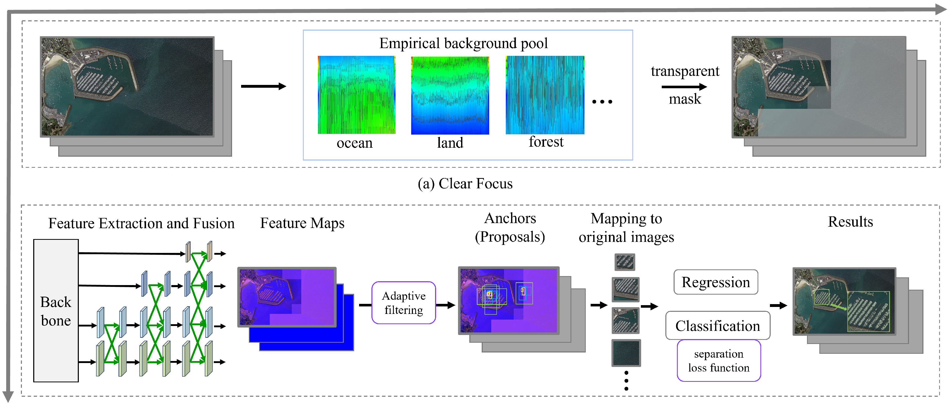
TMBO-AOD is composed of two primary components: the clear focus module and the adaptive filtering framework. As depicted in Figure 2, the clear focus module (Figure 2a) segments the input image into a predefined number of sub-blocks. Each sub-block is then compared to an empirical background pool. Sub-blocks identified as the background are assigned transparent masks to mitigate the influence of the background features. The adaptive filtering framework (Figure 2b) seamlessly integrates with both anchor-free and anchor-based methods, facilitating feature extraction and fusion. The adaptive filtering framework dynamically creates a varying number of candidate frames by analyzing the background and foreground sub-blocks that have been processed by the transparent masks. This process ensures a balance between positive and negative samples, thereby enhancing the optimization of the label assignment process. It is worth noting that the concept of an anchor does not exist in the anchorless model, in which case, an anchor is analogous to a proposal. For the sake of the uniformity of the expression, we unify anchors or proposals as candidates. Ultimately, TMBO-AOD yields accurate detection results.

2.1. Clear Focus Module

The clear focus module (CFM) comprises two main components: an empirical background pool and a transparent mask generation module.

2.1.1. Empirical Background Pool

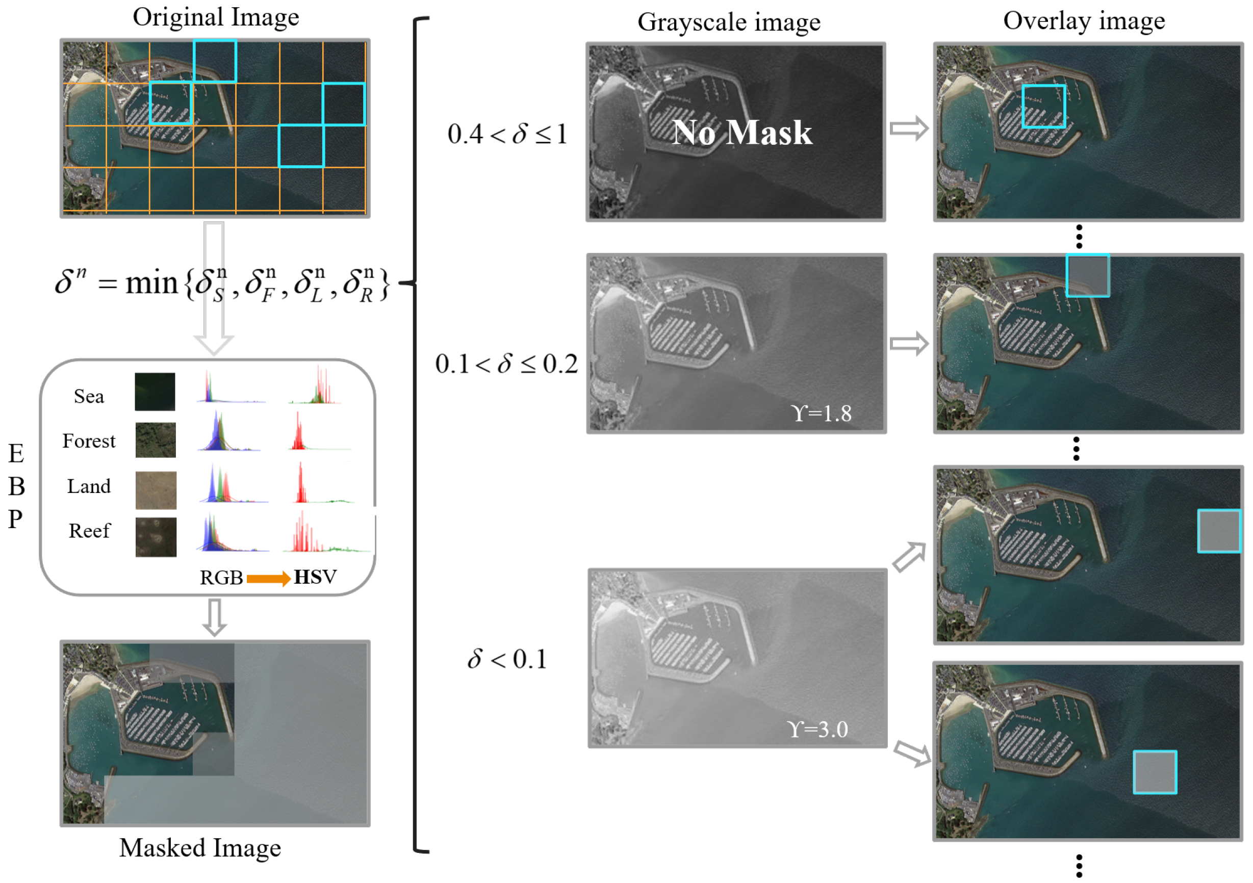
As illustrated in Figure 3, our study selected a total of one hundred representative images, with twenty-five images from each of the four predominant remote-sensing background categories: ocean, land, forest, and rock. This carefully curated selection achieves an optimal balance between diversity coverage and computational practicality. Although expanding the dataset could marginally improve the statistical precision, our empirical analysis confirms that the one hundred images in these four basic categories effectively capture the essential background characteristics in most remote-sensing scenarios.

The RGB color space directly encodes the intensities of the red, green, and blue channels but is highly sensitive to lighting variations. In contrast, the HSV color space provides better color consistency under changing illumination conditions. To mitigate illumination effects, we converted the collected RGB background images to HSV background images and computed the means and standard deviations of the hue (H) and saturation (S) channels, excluding the brightness channel to further reduce the sensitivity to lighting changes. These statistical values were then used to construct Gaussian distributions, which form the empirical background pool (EBP).

Because the background pool is highly data dependent, it must be recalculated when applied to a different dataset to ensure accuracy. For remote-sensing imagery, the existing four background types are typically sufficient. However, for datasets with different scene compositions, resampling is necessary to capture dataset-specific background characteristics. Fortunately, although resampling is required, the computation of statistical values remains straightforward. Moreover, leveraging prior background classification can significantly improve the efficiency of remote-sensing image interpretation. By first identifying the dominant background type in a given image, the number of unnecessary computations in irrelevant regions can be reduced, allowing detection algorithms to focus on areas with higher probabilities of containing targets. This background-aware processing strategy not only accelerates inferences but also enhances detection accuracy by mitigating false positives in uniform background regions. The formulae for computing the mean and variance from the H and S channels are as follows:

$${\overline{\mu }}_h={\displaystyle \frac{1}{M}}\sum _{j=1}^M({\displaystyle \frac{1}{N}}\sum _{i=1}^N{h}_i)$$

(1)

$${\overline{\sigma }}_h={\displaystyle \frac{1}{M}}\sum _{j=1}^M({\displaystyle \frac{1}{N}}\sum _{i=1}^N(h_i-{\overline{\mu }}_h))$$

(2)

$${\overline{\mu }}_s={\displaystyle \frac{1}{M}}\sum _{j=1}^M({\displaystyle \frac{1}{N}}\sum _{i=1}^N{s}_i)$$

(3)

$${\overline{\sigma }}_s={\displaystyle \frac{1}{M}}\sum _{j=1}^M({\displaystyle \frac{1}{N}}\sum _{i=1}^N(s_i-{\overline{\mu }}_s))$$

(4)

where M represents the number of images, N represents the total number of pixels in the channel, $h_i$ represents the value of the ith pixel in the Hth channel, $s_i$ represents the value of the ith pixel in the Sth channel, ${\overline{\mu }}_h$ represents the mean value of the Hth channel, ${\overline{\sigma }}_h$ represents the standard deviation of the H-th channel, ${\overline{\mu }}_s$ represents the mean value of the Sth channel, and ${\overline{\sigma }}_s$ represents the standard deviation of the S-th channel.

The formulae for establishing Gaussian distributions for H and V for the four backgrounds are as follows:

$$X\sim \mathcal{N}({\overline{\mu }}_X,{\overline{\sigma }}_X^2),X\in \{H_{\mathrm{ocean}},H_{\mathrm{land}},H_{\mathrm{forest}},H_{\mathrm{rock}}\}$$

(5)

$$Y\sim \mathcal{N}({\overline{\mu }}_Y,{\overline{\sigma }}_Y^2),Y\in \{S_{\mathrm{ocean}},S_{\mathrm{land}},S_{\mathrm{forest}},S_{\mathrm{rock}}\}$$

(6)

where X and Y are random variables representing the hue and saturation, respectively. $H_{\mathrm{ocean}}$, $H_{\mathrm{land}}$, $H_{\mathrm{forest}}$, $H_{\mathrm{rock}}$, $S_{\mathrm{ocean}}$, $S_{\mathrm{land}}$, $S_{\mathrm{forest}}$, and $S_{\mathrm{rock}}$ represent the Gaussian distributions of the H characteristics and S characteristics of the four types of backgrounds: ocean, land, forest, and reef, respectively.

The Gaussian distributions of the H and S channels for the four types of backgrounds are stored in the EBP. The input image will be divided into several sub-blocks based on a uniform rule. Specifically, the shorter side of the image is rounded up to 100 (with any excess not processed). This dimension is then divided by two and four to derive the side lengths of the square sub-blocks. The image will subsequently be partitioned into these square sub-blocks, while regions that cannot be fully covered by the sub-blocks will not be processed. In addition, the coordinates of the four vertices of each sub-block in the original image will be recorded. When the target image is divided into sub-blocks, the H and S channel means and variances of each sub-block are calculated to construct their respective Gaussian distributions (similar to those in (1)–(6)) as $I_H$ and $I_S$. These distributions are then compared with those in the EBP by computing the Wasserstein distance. The shortest average Wasserstein distance across the H and S channels is denoted as $\delta$ and is calculated using the following formulae:

$$W(I_H,X)=|{\overline{\mu }}_X-{\mu }_{I_H}|+\sqrt{{\overline{\sigma }}_X^2+{\sigma }_{I_H}^2}$$

(7)

$$W(I_S,Y)=|{\overline{\mu }}_Y-{\mu }_{I_S}|+\sqrt{{\overline{\sigma }}_Y^2+{\sigma }_{I_S}^2}$$

(8)

$$\delta =min({\displaystyle \frac{W(I_H,X)+W(I_S,Y)}{2}})x$$

(9)

where $I_H$ and $I_S$ are random variables based on the Gaussian distribution representing the characteristics of the sub-block in the H and S channels, respectively; W is the Wasserstein distance; and $\delta$ is the average distance obtained by comparing the Gaussian distribution of the image’s sub-block with those of the four backgrounds in the EBP, the shorter the distance, the more similar the sub-block is to a particular background. Sub-blocks with $\delta <1$ (an empirically determined threshold) are classified as background and assigned a corresponding flag, where 0 represents the background and 1 represents the foreground.

2.1.2. Transparent Mask

While comparing the image’s sub-blocks with those of the empirical background pool, a transparent mask is applied to the sub-blocks to minimize the interference of the background features in the target detection. The traditional approach directly adds a transparent channel based on semantic understanding, which can hinder compatibility with various target detection methods. However, we simulate transparency by superimposing a grayscale image onto the original image and adjusting its brightness using gamma correction. The gamma correction formula is as follows:

$$O=I^{\gamma }$$

(10)

where I is the pixel value in the input image, o is the pixel value after the gamma correction, and $\gamma$ is the gamma value, the higher the value, the brighter the image. Specifically, when $\delta <0.1$, indicating a high probability of the sub-block being a background block, the luminance value corresponding to $\gamma =3$ is applied. High-brightness grayscale maps can attenuate background features. For $0.1<\delta \le 0.2$, $\gamma$ is set at 1.8. There is a medium likelihood that the $\delta$ value in this range corresponds to the background, which will be superimposed onto a medium-brightness grayscale map. Sub-blocks of $\delta$ outside these ranges have a high probability of being the foreground, so no transparency mask is applied. Through this process, the resulting image is effectively refined to focus on the target regions, enhancing the detection performance.

2.2. Adaptive Filtering Framework

The adaptive filtering framework (AFF) and the CFM (Section 2.1) together form the core of the TMBO-AOD architecture. This two-stage filtering system first reduces the background interference at the pixel level through the CFM and then optimizes candidate generation at the detection level using the AFF, significantly enhancing the precision and speed of the target localization.

The CFM is primarily responsible for background-aware filtering, suppressing background noise and enhancing the foreground signal. Building upon this, the AFF broadens the focus by optimizing candidate generation at the detection level. This involves filtering out irrelevant background proposals and refining the selection of high-quality candidates, ensuring that only the best candidates are passed to the subsequent classification and regression stages.

Anchor-based and anchor-free detection paradigms fundamentally differ in their approaches to candidate generation and label assignment. Anchor-based methods rely on a predefined set of anchors with fixed sizes and aspect ratios, which provide a structured and straightforward approach for localizing objects. However, this rigidity can limit flexibility, as these fixed anchors may struggle to adapt to objects of varying scales and shapes. In contrast, anchor-free methods avoid using fixed anchors entirely, instead generating dynamic “virtual anchors” (commonly referred to as proposals) directly from the feature maps. This allows for more adaptive and context-aware candidate generation, which can be especially beneficial when dealing with complex or highly variable objects.

Given these fundamental differences, our AFF framework accommodates both paradigms, each with its unique candidate generation strategy. To standardize the terminology in this paper, we refer to the candidate boxes used for predicting the positions and categories of objects as “candidates”, which encompass both the fixed anchors used in anchor-based methods and the dynamically generated proposals of anchor-free approaches. Below, we describe the implementation of the AFF for both detection paradigms, highlighting how background flags are leveraged to optimize candidate generation and improve the detection performance.

2.2.1. Anchor-Based Methods

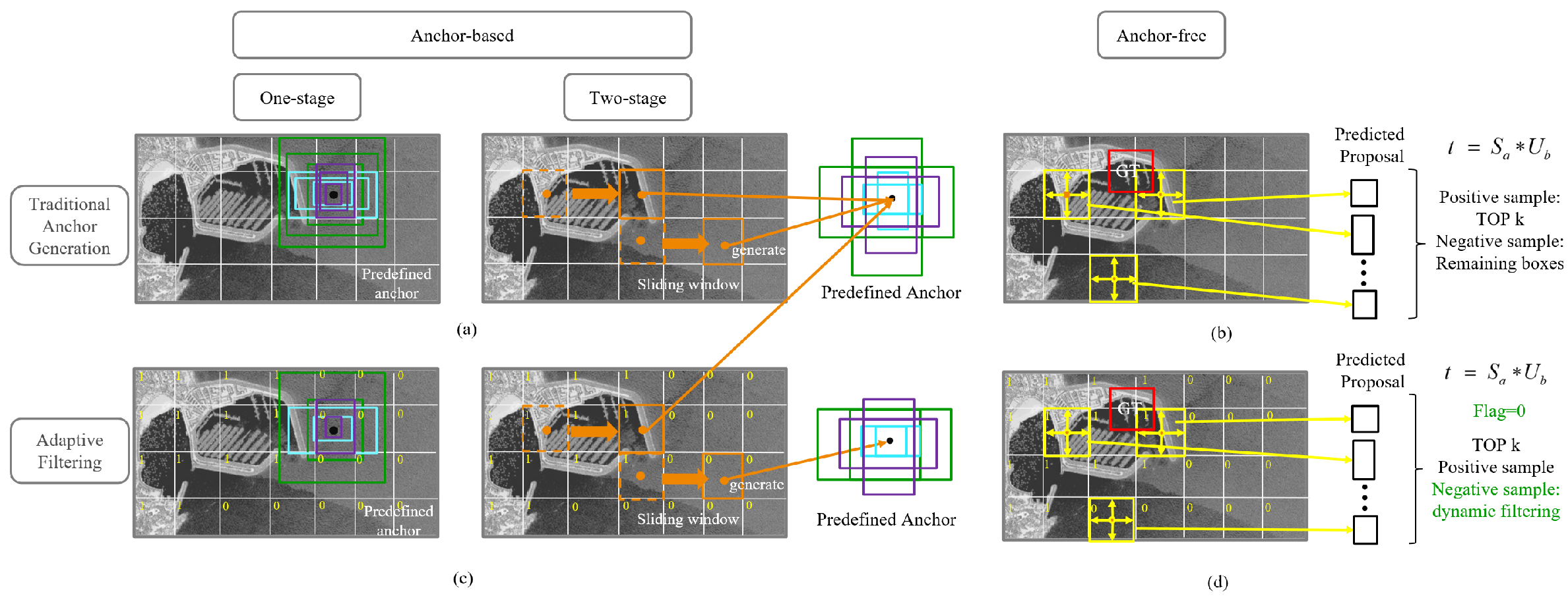
The most representative anchor-based methods include the single-stage YOLO series [15] and the two-stage faster R-CNN series [19]. Both utilize anchors of varying sizes and ratios to guide detection models in learning true object bounding boxes, although the anchor generation strategies differ. As shown in Figure 4a, for the last feature map layer in the detection, YOLO uses preset anchor sizes, and if these sizes deviate significantly from the true values, clustering is applied to regenerate fixed-sized anchors, which are then used across all the grid cells in the feature map. Faster R-CNN employs a regional proposal network (RPN) to generate anchors using a sliding window approach with three scales and three aspect ratios. As shown in Figure 4c, in our adaptive filtering detection framework, the background flag of the sub-block in the region where the center of the grid cell or the center of the window is located is determined before generating anchor points. Using this information, the number of anchors is dynamically adjusted: If the background flag is 0 (indicating a high probability of being the background), the number of anchors is reduced (e.g., from nine to six). If the background flag is 1, the anchor count remains unchanged. Both anchor-based methods classify positive and negative samples based on IoU thresholds. Most anchors generated in background regions are assigned as negative samples. However, with adaptive filtering, the number of negative samples is significantly reduced, addressing the issue of imbalanced positive and negative samples and effectively improving the velocity of the model’s operation.

2.2.2. Anchor-Free Methods

Our framework also offers a potential label assignment strategy for anchor-free methods. Taking YOLOv8 as an example, its label assignment is based on the task-aligned one-stage object detection (TOOD) [57] strategy. As illustrated in Figure 4b, YOLOv8 treats each grid in the feature map as a proposal and predicts the offsets of the four bounding box edges relative to the grid center. Positive samples are defined as those meeting the following criteria: The predicted box center lies within the ground truth (GT), and the IoU exceeds a predefined threshold. A ranking score, $t=S_a\ast U_b$, is used, where $S_a$ represents the category prediction score, $U_b$ is the IoU value, and a and b are hyperparameters. The top-K positive samples (default K = 13) are selected, while others are treated as negative samples. If multiple GTs correspond to a single proposal, the GT with the highest IoU is selected. Prior to this process, our AFF enhances the allocation of positive and negative samples using background flags, as shown in Figure 4d. Specifically, if a proposal originates from a grid with a background flag of 0, a method similar to “dropout” is applied to probabilistically discard the proposal. This approach effectively reduces the number of negative samples without causing imbalances because of excessive sample elimination.

Together with the CFM, the AFF forms the backbone of the TMBO-AOD architecture, providing a two-layer filtering mechanism that first removes irrelevant background information and then refines candidate selection. This dual-level optimization directly contributes to the high detection accuracy observed in our experiments, especially in complex background scenarios, where conventional methods struggle.

2.3. Separable Loss Function

The separable loss function (SLF) is a classification loss specifically designed to enhance the performance of object detection models by explicitly distinguishing between background and foreground regions, thereby enabling the model to learn to differentiate between these regions more effectively. This distinction contributes to both improving feature consistency and enhancing detection accuracy for both foreground objects and background features. The loss function integrates the focal loss ($FL$) for foreground classification with a custom background loss (${Loss}_{BG}$) to more effectively address background regions. The formulae for the classification loss (${Loss}_{cls}$) and background loss are presented below:

$$\begin{array}{cc}\hfill {Loss}_{cls}=& \sum _i(y_i·{\lambda }_0·FL(p_i,y_i))\hfill \\ \hfill & +(1-y_i)·({\lambda }_1·{Loss}_{BG}(f_i))\hfill \end{array}$$

(11)

where $p_i$ is the predicted probability for the target class, $y_i$ indicates whether the detection box is in a foreground region ($y_i=1$) or a background region ($y_i=0$), and ${\lambda }_0$ and ${\lambda }_1$ are weights controlling the balance between foreground and background learning.

2.3.1. Foreground Loss ($y_i=1$)

In foreground regions, the SLF uses the focal loss to focus on challenging samples and reduce the influence of easily classified background elements as follows:

$$FL(p_i,y_i)=-{(1-p_i)}^{\theta }log(p_i)\mathrm{if}{y}_i=1$$

(12)

The Focal Loss ($FL(p_i,y_i)$) is effective for addressing class imbalance by assigning higher importance to hard-to-classify samples, which is particularly useful in complex remote-sensing imagery.

2.3.2. Background Loss ($y_i=0$)

In background regions, the SLF incorporates a background loss that measures the similarity between the feature vector ($f_i$) of each region and a reference background vector (${\overline{f}}_{BG}$) from the empirical background pool. This loss is defined as follows:

$$Los{s}_{BG}=\alpha ·\sqrt{\parallel f_i-{\overline{f}}_{BG}{\parallel }^2}+(1-\alpha )·\left(1-{\displaystyle \frac{\langle f_i,{\overline{f}}_{BG}\rangle }{\parallel f_i\parallel ·\parallel {\overline{f}}_{BG}\parallel }}\right)$$

(13)

where $f_i$ is the feature vector of the ith region (typically the output from the last convolutional layer), ${\overline{f}}_{BG}$ is the mean feature vector representing typical background features, and $\alpha \in (0,1)$ balances the contributions of the two terms. The first term captures the overall distance between $f_i$ and ${\overline{f}}_{BG}$, using the Euclidean distance, helping the model to identify regions that deviate significantly from the background distribution. This is particularly useful for separating object-like structures from typical background noise. The second term uses cosine similarity to measure the alignment of feature vectors, focusing on their direction rather than just their magnitude. This helps to distinguish features that share similar spatial structures but differ in the semantic content, reducing the risk of false positives.

Together, these two components guide the model to learn a more precise background representation, improving its ability to differentiate foreground objects from complex background regions.

At this point, the important components of the TMBO-AOD have been introduced. It is important to highlight that the improvements offered by the TMBO-AOD are not confined to remote-sensing data; TMBO-AOD can be broadly applied to various types of datasets. In numerous computer vision tasks, such as autonomous driving, video surveillance, and medical image analysis, challenges like background interference and sample imbalance are equally significant. Consequently, dynamically generating candidate frames in the AFF and incorporating the background flags obtained from the CFM can effectively improve the detection accuracy and efficiency in these fields. By adjusting the candidate frame generation strategy and combining it with the SFL, the TMBO-AOD can be better aligned with the target features in different scenes, which significantly improves its detection performance in different datasets.

3. Global Experiments

3.1. Datasets

We evaluate the TMBO-AOD in four datasets: AI-TODv2.0, DIOR, DOTAv1.5, and NWPU VHR-10. AI-TOD contains 700,621 object instances across 28,036 aerial images, spanning 8 distinct categories. Compared to other aerial image object detection datasets, the average object size in AI-TOD is approximately 12.8 pixels, significantly smaller than the objects in other datasets. DIOR is a standard dataset for object detection in remote-sensing imagery, designed to offer a rich set of labeled data for detecting various targets. The dataset includes both high-resolution and low-resolution images, with target categories such as buildings, roads, vehicles, pedestrians, and more. It is widely used in fields like remote-sensing image analysis, target detection, and automated monitoring. DOTA is a large-scale, high-resolution aerial image dataset, comprising 2806 aerial images from 15 cities and regions, with a total of 188,282 annotated objects. These objects span multiple categories, including airplanes, ships, vehicles, basketball courts, and others. The NWPU VHR-10 dataset is a challenging ten-class geospatial object detection dataset. The dataset contains a total of 800 VHR optical remote-sensing images, of which 715 color images were obtained from Google Earth, with spatial resolutions ranging from 0.5 to 2 m. Eighty-five sharpened color–infrared images were acquired from the Vaihingen data, with a spatial resolution of 0.08 m. This dataset contains a total of 1000 VHR optical remote-sensing images.

3.2. Evaluation Metrics

The evaluation metrics used in the experiment are the average precision (AP), mean average precision (mAP), candidate generation time (CGT), and number of floating-point operations per second (FLOPS).

AP and mAP are commonly used metrics in the field of object detection. The formulae for calculating AP and mAP are as follows:

$$\mathrm{AP}={\int }_0^{1}P(R)dR$$

(14)

$$\mathrm{mAP}={\displaystyle \frac{1}{N}}\sum _{i=1}^N{\int }_0^{1}A{P}_i$$

(15)

where $P(R)$ represents the precision–recall curve, R is the recall, and N denotes the total number of object categories in the dataset. AP is computed by integrating the precision–recall curve over recall values from 0 to 1, reflecting the model’s ability to balance precision and recall across different confidence thresholds. The mAP is obtained by averaging the AP values across all the object categories, providing an overall measure of the detection accuracy. Specifically, AP and mAP are categorized as $A{P}_{50}$, $mA{P}_{50}$, $A{P}_{75}$, $mA{P}_{75}$, $A{P}_{50-95}$, $mA{P}_{50-95}$, $A{P}_{vt}$, $A{P}_t$, $A{P}_s$, and $A{P}_m$. $A{P}_{50}$, $A{P}_{75}$, and $A{P}_{50-95}$ are the average precision scores calculated over the IoU ranges 0.5, 0.75, and from 0.5 to 0.95, respectively. Furthermore, $mA{P}_{50}$, $mA{P}_{75}$, and $mA{P}_{50-95}$ are the mean values of the APs for each category, calculated over the IoU ranges 0.5, 0.75, and from 0.5 to 0.95, respectively. Additionally, $A{P}_{vt}$, $A{P}_t$, $A{P}_s$, and $A{P}_m$ are the APs of very tiny (2–8 pixels), tiny (8–16 pixels), small (16–32 pixels), and medium-sized (32–64 pixels) objects defined in the AI-TOD dataset. The calculation methods of the AP and mAP are similar but differ in their specific applications and interpretations. Therefore, for different comparison experiments, we choose either AP or mAP as an evaluation index according to the real situation.

In addition, CGT is the time (in seconds) required to generate candidate boxes in the target detection task. CGT depends on the complexity of the generation algorithm and affects the velocity and accuracy of the target detection system. A shorter candidate generation time indicates a more efficient detection framework. Furthermore, FLOPS values are included as a metric for the computational complexity, reflecting the number of floating-point operations required for inferences. Lower FLOPS values indicate reduced computational costs, which are critical for real-time and resource-constrained applications.

3.3. Implementation Details

We propose two versions of the TMBO-AOD for comparative and ablation studies: TMBO-AOD5, based on YOLOV5, and TMBO-AOD8, based on YOLOV8. The former serves as an anchor-based model, while the latter functions as an anchor-free model, with notable differences in their feature extraction and feature fusion components. The generalization of the TMBO-AOD can be demonstrated through comparisons of both versions of the model with classical object detection models and the current outstanding model. The TMBO-AOD framework is an empirical-background-pool-based screening detection framework, allowing for the replacement of both the backbone network and the feature fusion network according to specific requirements. The TMBO-AOD is implemented in PyTorch 2.0 and operates on a system equipped with two NVIDIA 4090 GPUs. The model is trained using distributed data parallel (DDP) to enhance the training efficiency, achieving twice the velocity relative to that for training on a single GPU. Our designed model did not utilize any pretrained weights during the training process. The training process is optimized using SGD, with momentum parameters ${\beta }_1=0.9$ and ${\beta }_2=0.95$, and cosine decay was employed, with a base learning rate of 3.75 × 10⁻⁵. Random scaling, random cropping, and random horizontal flipping are also employed. Additionally, the input image’s size is standardized to 1280 × 1280 pixels. Unless otherwise stated, all the comparison methods in the experiments utilized the official code, and all the settings are consistent with those provided in the official documentation.

3.4. Comparisons with the SOTA Methods

3.4.1. Experiment with AI-TODv2.0

In

Table 1. A comparison of the detection results with those of the state-of-the-art models in AI-TODv2.0. All the AP values in the table are expressed as percentages, but this is omitted for clarity. Note that the red numbers refer to the best results, the blue numbers refer to the second best results.

Method	Venue	AP50–90	AP50	AP75	APvt	APt	APs	APm	GFLOPS
Faster R-CNN	TPAMI2017	12.7	25.7	7.4	0.0	11.6	28.3	33.9	289.3
DETR [58]	ECCV2020	2.9	11.7	0.5	0.6	2.6	3.3	12.1	227
iRMB [64]	ICCT2021	21.3	44.7	19.9	5.0	23.9	33.8	53.9	57.1
IQDet [59]	CVPR2021	9.4	21.7	11.3	2.1	9.2	15.6	31.8	68.4
DetectoRS [60]	CVPR2021	15.0	32.6	12.1	0.1	10.6	28.9	40.0	244
Swin Transformer–tiny [61]	ICCV2021	9.7	24.4	5.3	5.4	10.4	15.3	24.8	105.2
Swin Transformer–sin [61]	ICCV2021	12.9	32.7	6.2	6.7	10.1	20.9	37.6	11.8
MSC [65]	NeurIPS2022	21.4	42.7	17.1	9.1	15.5	29.1	47.9	32.8
RFLA [54]	ECCV2022	24.1	55.5	18.7	9.6	25.8	30.1	37.6	-
NWD [66]	ISPRS2022	23.9	54.6	16.9	8.9	24.1	29.2	36.5	246
LSK [67]	CVPR2023	21.2	43.4	17.7	10.0	15.6	30.3	53.9	63.4
YOLOv8s [62]	arXiv2023	15.4	36.1	20.3	4.1	11.9	35.5	45.9	29.7
BRSTD [68]	TGRS2024	23.6	54.2	16.6	10.4	22.8	30.3	37.6	64.3
YOLOv9s [63]	arXiv2024	21.7	42.6	22.2	4.9	11.6	37.0	51.4	67.7
HANet [69]	TCSVT2024	24.0	53.7	19.8	10.3	22.2	27.3	55.5	171.3
TMBO-AOD5 (Ours)	-	22.4	49.9	22.8	9.9	26.5	32.7	52.8	55.9
TMBO-AOD8 (Ours)	-	24.4	56.1	23.8	10.9	38.1	35.1	54.9	123.2

Note that red refers to the best results and blue refers to the second best results. Because of the limited space in the table, the percentage symbol (%) is omitted from all the AP values.

, we compare the performances of the two versions of the TMBO-AOD (TMBO-AOD5 and TMBO-AOD8) with those of other baseline models in the AI-TODv2.0 test set. These baseline models include the mainstream methods in computer vision: faster R-CNN, DETR [58], IQDet [59], DetectoRS [60], a Swin Transformer [61], YOLOv8 [62], and YOLOv9 [63], as well as the remote-sensing image-oriented SOTA models, iRMB [64], MSC [65], RFLA [48], NWD [66], LSK [67], BRSTD [68], and HANet [69].

Overall, TMBO-AOD8 outperforms the current leading methods across multiple metrics, demonstrating substantial performance advantages. Specifically, TMBO-AOD8 achieves 24.4%, 56.1%, and 23.8% increases in detection accuracy for AP_50–90, AP₅₀, and AP₇₅, respectively, representing improvements of 0.3% for AP_50–90, 0.6% for AP₅₀, and 5.1% for AP₇₅ compared to the detection performances of the second highest performing model, RFLA [64]. In terms of the detection performances for small AP_s = 35.1) and medium-sized (AP_m = 54.9) targets, TMBO-AOD8 demonstrates a significant advantage over the third highest performing model, HANet [69], with an improvement of 7.8% for AP_s. Although the detection performance for AP_m is slightly lower than that for HANet, it ranks second among all the models. Furthermore, compared to the computational complexity of the most parameter-efficient model, the Swin Transformer [61] (11.8 GFLOPS), that of TMBO-AOD8 is in the medium range (123.2 GFLOPS), yet TMBO-AOD8 significantly enhances the detection performance, particularly in detecting both very small targets (AP_vt = 10.9) and tiny targets (AP_t = 38.1), outperforming all the other models. Conversely, the lightweight TMBO-AOD5 model exhibits a more advantageous computational complexity of only 55.9 GFLOPS, although its detection performance is slightly lower than that of TMBO-AOD8. The TMBO-AOD5 model achieves 22.4% and 49.9% increases in detection accuracy for AP_50–90 and AP₅₀, respectively, outperforming those of recent high-performing models, such as NWD [58] and BRSTD [61], as well as all the other models in small-target detection. It also achieves the second highest accuracy (26.5%) in tiny-target detection, demonstrating exceptionally high parametric efficiency. Compared to the lightweight model, YOLOv9 [63] (67.7 GFLOPS), the TMBO-AOD5 model exhibits lower computational complexity while demonstrating higher detection accuracy across nearly all the metrics.

In summary, our models achieve an exceptional balance between computational efficiency and detection accuracy. TMBO-AOD5 delivers a 22.4% improvement in detection accuracy for AP_50–90 at just 55.9 GFLOPS, demonstrating remarkable computational efficiency. Although TMBO-AOD8 increases the computational load to 123.2 GFLOPS (2.2× higher than that of TMBO-AOD), it provides only a 9% relative improvement in detection accuracy for AP_50–90 (24.4%), revealing clearly diminishing returns from simply scaling up the model size. In addition, TMBO-AOD5’s 55.9 GFLOPS computational demand is fully in line with the real-time processing power of mainstream edge processors (in the 50–100 GFLOPS range), which enables TMBO-AOD5 to be effectively deployed in edge devices. In the future, we will further validate this capability to ensure its feasibility in resource-constrained environments.

3.4.2. Experiment with DOTAv1.5

In this experiment, we use the DOTAv1.5 dataset with the “train” set for training and the “val” set for testing. In addition to the models listed in Table 1, we compare TMBO-AOD8 with several other baseline models, including the classic visual domain model MobileNet [70], FasterNet [71], and the remote-sensing object detection domain models TOSO [72], GWD [73], BDR-Net [74], and O²DFFE [75].

As shown in

Table 2. Comparison of detection results with those of state-of-the-art models in the DOTAv1.5 dataset.

Method	Venue	AP50 (%)																mAP50 (%)
		PL	SH	ST	BD	TC	BC	GTF	HA	BR	LV	SV	HC	RA	SBF	SP	CC
Faster R-CNN [19]	TPAMI2017	81.9	77.5	84.3	73.1	90.6	76.1	58.7	61.1	43.9	70.9	72.6	56.8	63.1	48.0	71.1	20.2	63.7
MobileNet [70]	CVPR2019	74.8	32.4	17.3	13.5	29.4	54.7	69.6	79.8	17.7	45.7	19.3	14.7	52.0	53.8	8.8	9.9	39.4
TOSO [72]	ICASSP2021	87.2	65.6	44.3	48.9	46.1	68.0	83.0	90.7	46.0	68.9	48.7	60.8	66.5	70.6	17.9	32.3	62.5
GWD [73]	PMLR2021	88.1	77.8	78.5	76.6	85.9	80.1	65.2	63.8	34.9	61.7	71.3	54.5	61.2	58.3	62.3	38.1	12.9
Swin Transformer–tiny [61]	ICCV2021	40.5	15.1	3.8	5.3	10.4	27.4	32.2	48.6	5.2	19.9	4.1	7.2	13.0	23.5	1.7	20.7	13.9
Swin Transformer–sin [61]	ICCV2021	42.1	10.2	3.4	1.3	13.2	25.8	35.6	48.0	5.7	24.9	3.6	6.0	15.1	21.0	1.5	22.1	23.1
AO2-DETR [76]	TCSVT2022	79.6	79.7	77.6	78.1	80.6	74.7	61.2	58.6	42.4	74.5	55.3	69.6	66.9	53.6	73.2	24.7	66.3
O2DFFE [77]	RS2022	80.2	86.1	82.3	81.5	90.8	79.2	72.0	73.4	53.5	80.9	67.5	66.8	60.3	60.1	73.1	25.7	70.8
FasterNet [71]	CVPR2023	47.2	19.6	8.3	6.4	14.5	30.5	41.6	60.7	8.1	26.5	9.3	14.7	19.0	25.8	2.6	18.9	69.3
YOLOV8s	arXiv2023	89.9	74.5	50.2	55.4	50.3	71.6	85.4	91.4	52.8	73.4	59.1	66.1	75.0	71.4	43.2	39.3	65.9
BDR-Net [74]	TIM2023	89.7	79.7	82.9	78.4	90.8	83.1	73.1	70.0	46.0	74.7	75.4	48.2	63.1	60.7	66.8	42.9	71.0
HANet [69]	TCSVT2024	90.5	71.2	49.2	47.8	52.5	73.3	85.6	90.9	57.6	74.3	51.0	66.3	75.6	75.6	42.7	40.1	65.9
TMBO-AOD8 (Ours)	-	90.8	88.1	84.3	75.2	84.9	89.2	85.0	92.5	58.0	81.5	79.7	74.2	76.6	72.9	76.4	44.8	78.1

Note that red refers to the best results and blue refers to the second best results.

, TMBO-AOD8 consistently outperforms all the other mainstream object detection models in the DOTAv1.5 dataset, achieving the highest overall mAP₅₀ of 78.1%, significantly ahead of the second-ranked BDR-Net (71.0%) and third-ranked O²DFFE (70.8%). Among the 16 object categories, TMBO-AOD8 achieves the best AP₅₀ in 12 categories, including complex scenarios, like basketball court (BC), where it leads by 6.1% over the second best model. This superior performance demonstrates the robustness of TMBO-AOD8 in handling dense targets and complex backgrounds, a key advantage provided by its CFM, which effectively reduces background interference by constructing an empirical background pool based on Gaussian distribution, allowing the model to concentrate more accurately on foreground targets.

Moreover, TMBO-AOD8 maintains strong performances in categories with high background complexity, such as swimming pools (SPs) and harbors (HAs), surpassing the second-place model’s performances by 3.2% and 1.1%, respectively. In challenging small-target detection, such as a small vehicle (SV) and a large vehicle (LV), TMBO-AOD8 also outperforms the other models by 4.3% and 0.6%, respectively. This is mostly attributed to the SLF, which enhances the model’s ability to distinguish foreground objects from complex backgrounds, further optimizing the overall detection performance.

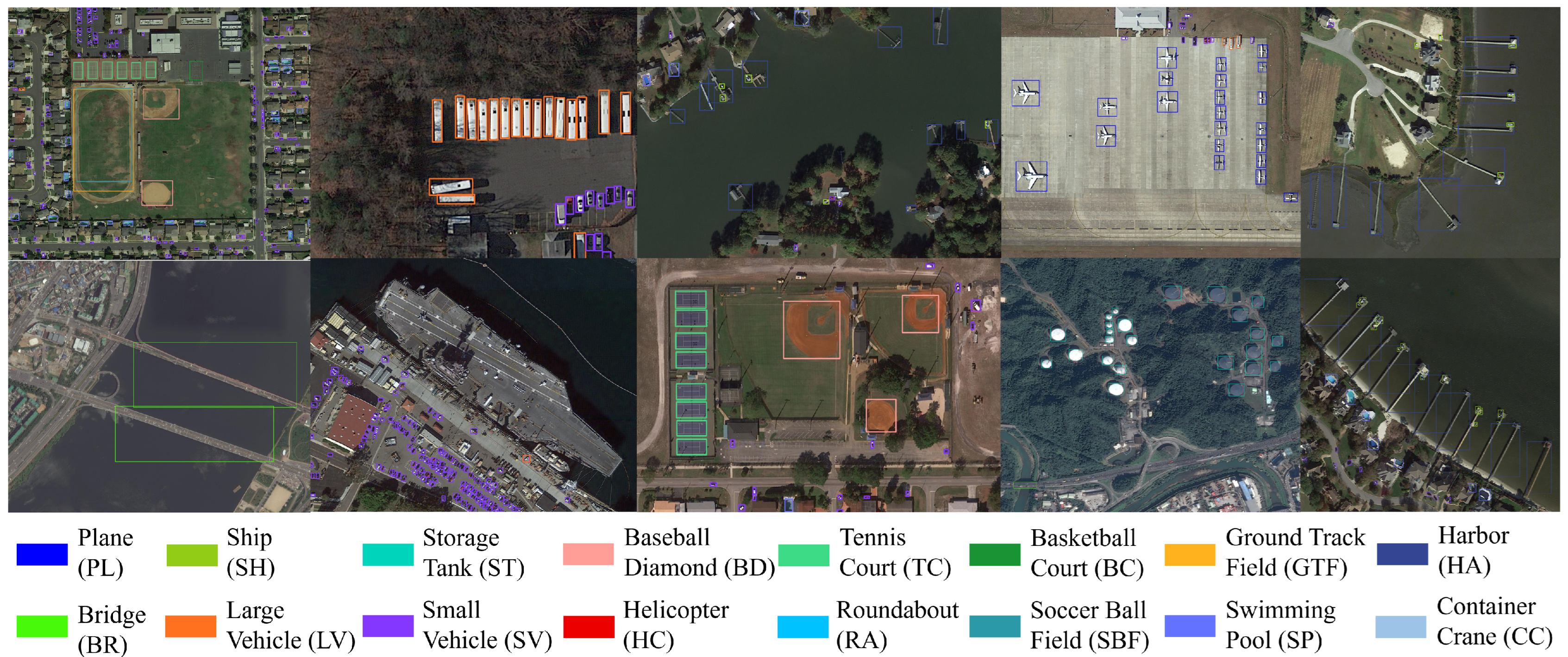
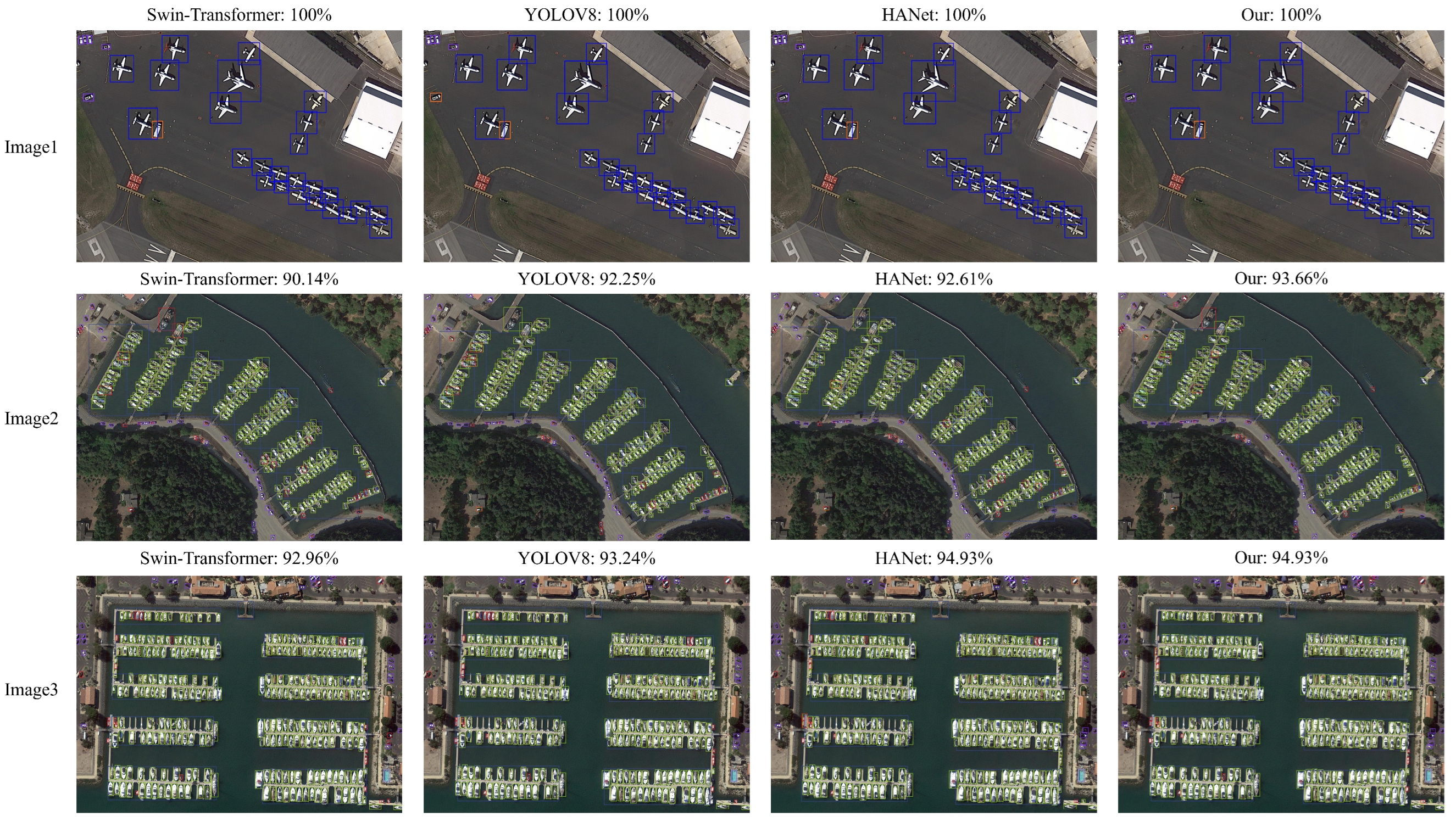
Importantly, compared to O²DFFE, which also focuses on mitigating background interference, TMBO-AOD8 demonstrates a more comprehensive approach to background suppression. Although O²DFFE relies on a keypoint attention mechanism and prototype contrastive learning to enhance the foreground, TMBO-AOD8 incorporates a more nuanced strategy through its CFM and SLF, effectively balancing positive and negative sample distributions and dynamically optimizing candidate generation, resulting in a more accurate and stable detection performance across various object scales and scene complexities. The partial inference results of TMBO-AOD8 in the DOTAv1.5 validation set are shown in Figure 5.

Additionally, we performed qualitative analyses on four models, with the visualization results presented in Figure 6. As shown, our TMBO-AOD8 model consistently achieved the highest detection accuracy across three randomly selected images. However, it is noteworthy that in the third image, the performance of TMBO-AOD8 did not exhibit a significant improvement compared to those of the other models. Upon further analysis, this may be attributed to the relatively small proportion of background regions in the image, limiting the effectiveness of the CLM and AFF modules, which are designed to optimize background suppression. Nevertheless, TMBO-AOD8 still demonstrated robust overall performance.

3.4.3. Experiment with DIOR

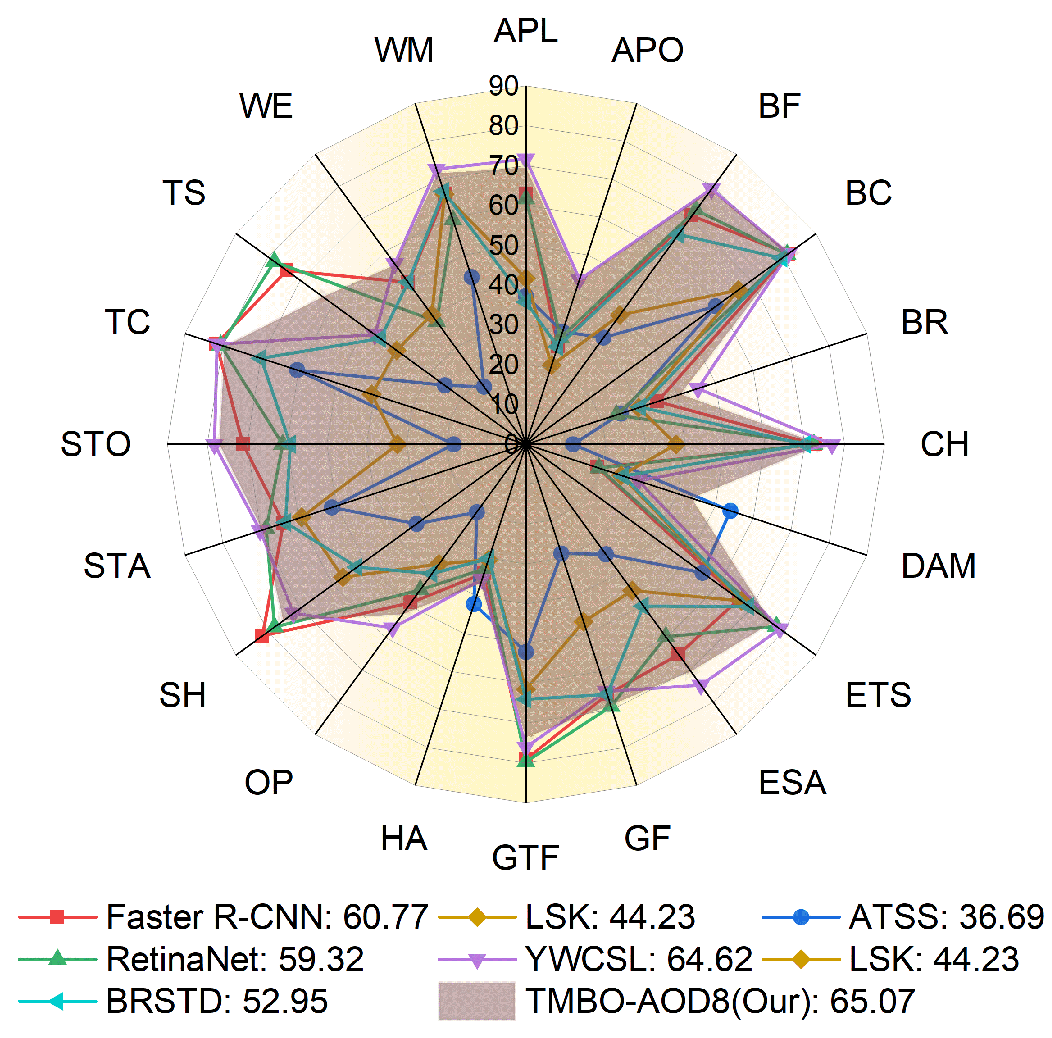
In this experiment, we compare the performance of TMBO-AOD8 with those of the other baseline models in the DIOR test set. Figure 7 shows the classification accuracies and average accuracies of TMBO-AOD8 and the other mainstream methods in the DIOR dataset, and it can be seen that TMBO-AOD8 significantly outperforms the other mainstream methods in the DIOR dataset and achieves the best overall performance, with a mAP of 65.07%, outperforming models such as Faster R-CNN (60.77%), RetinaNet (59.32%), and the other classical models. TMBO-AOD8 improves upon the sub-optimal model (YWCSL) by 0.45%. The radar plot reveals that TMBO-AOD8 performs well across most categories (e.g., “storagetank” (ST), “trainstation” (TS), and “airport” (APO)). These categories usually have complex backgrounds or contain small targets, showing the model’s adaptability in multi-scene and multi-target detection tasks. Meanwhile, in terms of the coverage area, TMBO-AOD8 is able to maintain a balanced high performance across categories, rather than excelling in only a few categories, demonstrating its comprehensiveness in the overall detection task. The model’s wide range of advantages can be attributed to its transparent mask and background optimization strategies, which effectively separate the target from the background by constructing empirical background pools with Gaussian distributions, especially in scenarios with complex backgrounds and confusing targets (e.g., “airport” and “harbor”), and greatly reducing the number of false positives. The adaptive filtering framework dynamically adjusts the number of candidates, which not only optimizes the detection efficiency but also significantly alleviates the positive and negative sample imbalance problem, thus improving the detection of small-target categories (e.g., “basketballcourt” (BC) and “windmill” (WM)). In addition, the separation loss function enhances the feature consistency between the foreground and background, which enables the model to maintain stable detection accuracy in diverse scenes.

3.4.4. Experiment with NUPUVHR-10

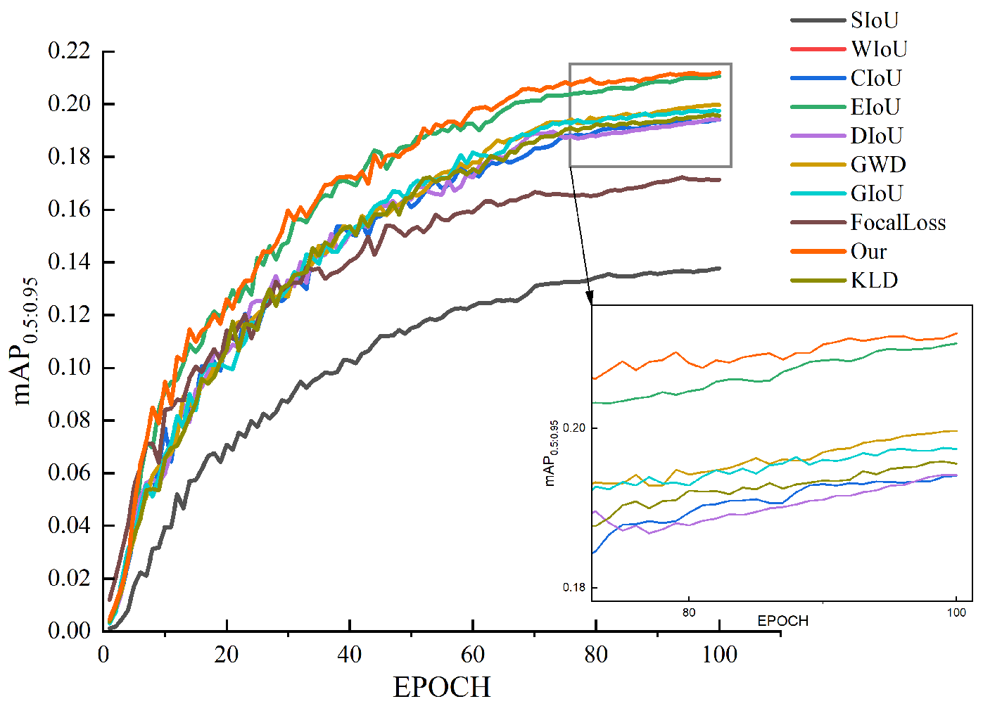
We used the NUPUVHR-10 dataset to compare several different loss functions, namely, the generalized loss functions DIoU [45], CIoU [46], EIoU [47], WIoU [48] and SIoU [49] for visual detection; focal loss [7] for small-target detection; and GWD [66] and KLD [77] for remote-sensing rotating-target detection. Because horizontal detection boxes can be viewed as a special case of rotating detection boxes (when the angle is 0°, 90°, or any multiple thereof), the fundamental principles of GWD and KLD remain applicable. Therefore, we also conduct a comparative analysis with GWD and KLD. Figure 8 illustrates the $mA{P}_{0.5:0.95}$ performance of the various loss functions over training epochs, demonstrating the superiority of our proposed SLF. Compared to traditional IoU-based losses such as SIoU, WIoU, and CIoU, which plateau at lower accuracy levels, the SLF continues improving, even in later training stages, achieving the highest final detection accuracy. Distribution-based losses, like GWD and KLD, show moderate improvements over IoU-based methods but still fall short of the SLF, while focal loss, despite its strength in handling class imbalances, remains slightly below the SLF, suggesting that explicitly modeling background information provides additional performance gains. The zoomed-in section further highlights how the SLF maintains a consistent advantage, demonstrating its ability to refine object detection through both foreground and background learning. Unlike conventional losses, which treat the background as a generic negative sample, the SLF integrates a focal-loss-based foreground optimization with a background loss component that explicitly models background features’ consistency, reducing the number of false positives and enhancing the detection’s robustness. Moreover, by leveraging an empirical background pool, the SLF refines the distinction between the foreground objects and background clutter, making it more effective in complex remote-sensing imagery. These combined factors enable the SLF to achieve superior detection accuracy, improved convergence stability, and better adaptability to challenging detection environments, making it a compelling alternative to conventional loss functions.

4. Discussion

4.1. Ablation Experiments Based on the Number of Sub-Blocks

To evaluate the impact of the TMBO-AOD framework on the detection accuracy for different sub-block configurations, we conducted ablation experiments on four datasets (DOTAv1.5, AI-TODv2.0, NUPUVHR-10, and DIOR) using anchor-based YOLOv5 and anchor-free YOLOv8. The results, as shown in

Table 3. The performances of YOLOv5 and YOLOv8 incorporating the TMBO-AOD without pretraining in the four datasets.

Method	Dataset	Sub-Blocks	AP50–90 (%)	AP50 (%)
YOLOV5	DOTAv1.5	0	39.09	63.29
		2	39.57	64.21
		4	41.96	66.95
	AI-TODv2.0	0	18.19	45.97
		2	18.36	46.25
		4	19.15	47.01
	NUPUVHR-10	0	58.23	94.19
		2	58.96	94.88
		4	59.27	95.30
	DIOR	0	19.87	48.58
		2	21.22	49.60
		4	22.57	53.13
YOLOV8	DOTAv1.5	0	39.27	63.89
		2	40.18	64.56
		4	42.12	68.17
	AI-TODv2.0	0	18.56	46.00
		2	19.37	46.34
		4	20.15	47.22
	NUPUVHR-10	0	59.67	95.82
		2	61.01	96.33
		4	61.75	98.21
	DIOR	0	20.35	49.77
		2	21.56	50.82
		4	22.34	54.97

Note that bold font represents optimal performance.

, indicate significant performance improvements across all the datasets when incorporating the TMBO-AOD framework. Notably, the configuration with four sub-blocks achieved the highest performance gains for both models.

Specifically, YOLOv5 exhibits the most substantial improvement in the DIOR dataset, with an AP₅₀ increase of 9.36% (from 48.58% to 53.13%) and an AP_50–90 increase of 13.58% (from 19.87% to 22.57%). For YOLOv8, the most remarkable improvement is observed in the DIOR dataset, achieving an AP₅₀ increase of 10.45% (from 49.77% to 54.97%) and an AP_50–90 increase of 19.63% (from 20.35% to 24.34%). Across all the datasets, the configuration with four sub-blocks consistently outperformed both the baseline (no sub-blocks) and the two-sub-block configuration, highlighting the robustness of the TMBO-AOD framework.

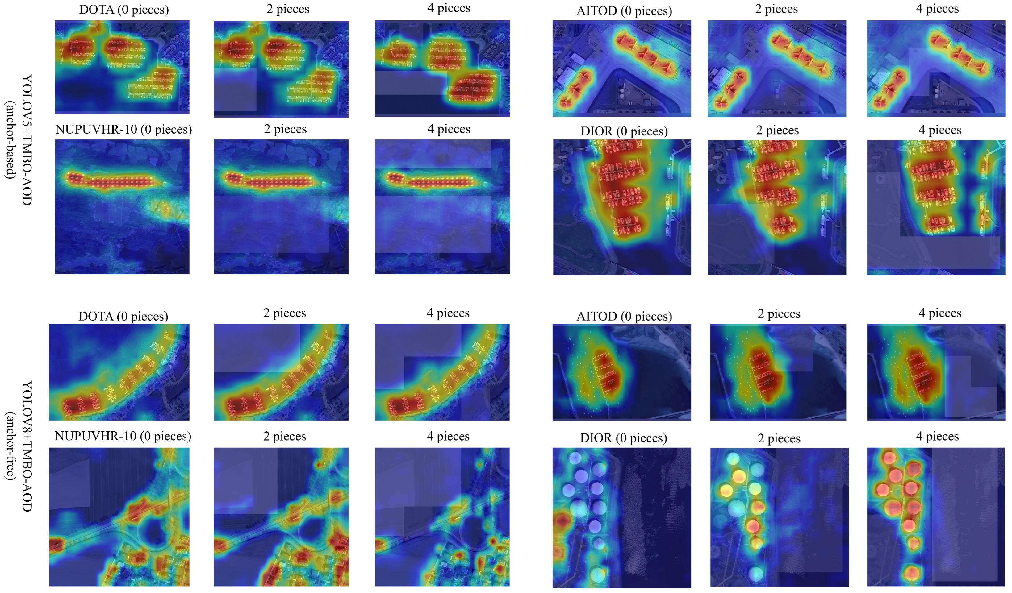
The heatmaps in Figure 9 visually illustrate the advantages of incorporating sub-blocks into the TMBO-AOD framework. Compared to the baseline YOLO models, the enhanced models with four sub-blocks demonstrate a more concentrated focus on target regions while effectively suppressing the background noise. The addition of transparent masks to sub-blocks, as a part of TMBO-AOD’s design, enables the models to isolate foreground targets and minimize interference from background regions. This effect is particularly evident in high-density datasets, like AI-TODv2.0, where dense and small targets are better localized with sharper boundary definitions.

The effectiveness of the four-sub-block configuration can be attributed to several key mechanisms within the TMBO-AOD framework. First, the adaptive filtering mechanism optimizes the balance between positive and negative samples, improving the detection accuracy for small and ambiguous boundary targets. Second, the separation loss function enhances the distinction between the foreground and background, as reflected in the heatmaps, where background regions consistently exhibit low responses, while target regions display clear and precise high-heat areas.

When the number of sub-blocks increases, the TMBO-AOD framework expands its masking area, further reducing the background interference and sharpening its focus on target regions. This trend is particularly pronounced in the DIOR dataset, where the baseline YOLOv8 often struggles to concentrate on targets, resulting in scattered high-response regions. In contrast, the TMBO-AOD-enhanced YOLOv8 with four sub-blocks achieves significantly improved target localization, as seen in Figure 9.

However, certain regions in the heatmaps reveal limitations in the TMBO-AOD framework’s performance. When targets are more dispersed, the framework can struggle to completely isolate all the background areas. In some cases, portions of the background sub-blocks may inadvertently capture parts of the targets, resulting in over-detection, where target objects are incorrectly classified as background elements. This effect is primarily because of the relatively large size of the sub-blocks, which can fail to effectively differentiate small, target-like background features from actual targets.

As demonstrated in Figure 9, increasing the number of sub-blocks from two to four significantly improves the separation of the foreground and background, allowing for finer-grained masking and more precise focus on target regions. However, this improvement comes at the cost of reduced model efficiency, as a greater number of sub-blocks requires more computational resources to process the finer distinctions between background and foreground regions. Additionally, this approach can sometimes lead to over-detection if the model starts to interpret fine background textures or isolated background objects as potential targets, thus reducing the overall precision.

Therefore, finding an optimal balance between the sub-block size and overall model performance is critical. This balance helps to avoid both efficiency losses and over-detection, ensuring that the model effectively isolates true foreground targets without being misled by background noise. We explore the effect of the sub-block size on the model’s performance in Section 4.1.

Further validation of the four-sub-block configuration is provided in

Table 4. The performances of YOLOv5 and YOLOv8 incorporating the TMBO-AOD without pretraining in the DIOR dataset.

Method	AP50–90 (%)	AP50 (%)	CGT (s)
YOLOV5	4.11	11.87	1.22
YOLOV5 + TMBO-AOD	6.75	17.68:	0.63 (↑48.36%)
YOLOV8	4.63	12.76	0.47
YOLOV8 + TMBO-AOD	7.92	19.20	0.25 (↑46.81%)

Note that upward arrow represents performance improvement and bold font represents optimal performance.

, which presents the performances of YOLOv5 and YOLOv8 in the DIOR dataset after 20 training epochs. The TMBO-AOD framework yields substantial accuracy improvements, with YOLOv5 and YOLOv8 achieving respective increases of 9.42% and 8.76%. Moreover, the framework significantly reduces the candidate generation time, with YOLOv5 achieving a 48.36% reduction and YOLOv8 a 46.81% reduction. These results highlight the dual benefits of the TMBO-AOD: enhanced detection accuracy and improved computational efficiency, making it highly suitable for real-world applications.

4.2. Ablation Experiments with Hyperparameters in the Loss Function

We tuned the untrained TMBO-AOD8 model in the AI-TODv2.0 dataset, as shown in

Table 5. Hyperparameter combinations and detection performance metrics in the AI-TODv2.0 dataset.

$\mathit{\alpha }$	$\mathit{\theta }$	${\mathit{\lambda }}_0$	${\mathit{\lambda }}_1$	AP50–90 (%)	AP50 (%)	AP75 (%)
0.5	2.0	1.0	1.0	19.60	47.73	18.25
		2.0	1.0	19.29	46.61	19.86
		1.0	2.0	19.83	49.15	20.26
		1.0	3.0	19.77	49.09	19.91
0.6	2.0	1.0	2.0	19.42	48.73	19.02
0.7				19.99	49.73	20.45
0.8				19.23	48.59	18.88
0.7	3.0	1.0	2.0	19.22	48.13	18.90
	4.0			19.12	48.25	19.70
	2.5			20.35	50.22	21.56

Note that bold font represents optimal performance.

, to identify the optimal hyperparameter settings for the SLF. This process involved two stages as follows:

First, we focused on the weighting parameters, ${\lambda }_0$ and ${\lambda }_1$, which balance the relative importance of the foreground and background components in the SLF. We fixed the values of $\alpha$ and $\theta$ and tested different combinations of ${\lambda }_0$ and ${\lambda }_1$. The results indicate that the model generally achieved better performance when ${\lambda }_0<{\lambda }_1$, with the optimal combination being ${\lambda }_0=1.0$ and ${\lambda }_1=2.0$. This configuration resulted in the highest overall performance, achieving AP_50–90 = 19.83%, AP₅₀ = 49.15%, and AP₇₅ = 20.26%. This outcome suggests that assigning a higher weight to the background loss helps the model to better capture the background features, effectively filtering out irrelevant regions and focusing on a smaller set of potential target regions.

Next, we fixed the optimal ${\lambda }_0$ and ${\lambda }_1$ values and explored the impact of the background-modeling parameter, $\alpha$, which controls the balance between the Euclidean distance and cosine similarity in the background loss function, on the detection accuracy. This balance is critical, as it influences how the model distinguishes subtle background variations. Our experiments revealed that setting $\alpha =0.7$ resulted in the best performance, likely because this configuration provides a balanced emphasis on both the feature magnitude and direction, enhancing the model’s ability to capture complex background patterns.

Finally, we refined the focal modulation parameter, $\theta$, and found that $\theta =2.5$ provided the best results. This value effectively balances the impacts of hard and easy samples, contributing to the overall detection performance.

After a series of ablation experiments, the optimal hyperparameter configuration was identified as $\alpha =0.7$, $\theta =2.5$, ${\lambda }_0=1.0$, and ${\lambda }_1=2.0$, achieving the best overall performance. This combination effectively balances the tradeoff between precise foreground classification and robust background filtering, resulting in a significant boost in detection accuracy across varying IoU thresholds.

4.3. Ablation Experiments with Contributions from Each Component

The ablation results in

Table 6. Ablation results for the various components in TMBO-AOD5.

CFM	AFF	SLF	mAP50–90	mAP50	mAP75	mAPvt	mAPt	mAPs	mAPm
			18.1	37.2	17.0	8.3	15.4	31.4	41.9
✓			19.7	38.4	18.2	8.3	15.9	32.3	43.7
✓	✓		20.2	39.4	17.6	8.0	16.8	32.5	45.2
✓		✓	21.5	43.5	21.9	9.3	19.7	32.4	51.4
✓	✓	✓	22.4	49.9	22.8	9.9	26.5	32.7	52.8

Note that bold font represents optimal performance. The check mark represents the adoption of the module.

highlight the impact of each core component within the TMBO-AOD5 framework on the detection accuracy. Given that the CFM serves as the foundational component for both the AFF and the SLF, the latter two cannot be independently evaluated. With only the CFM enabled, the model shows significant gains, boosting mAP_50-90 from 18.1% to 19.7% and mAP₅₀ from 37.2% to 38.4%, reflecting the effectiveness of empirical background pooling in reducing the background interference. This setup also improves mAP₇₅ from 17.0% to 18.2%, indicating more precise boundary localization. Adding the AFF further enhances medium-scale target detection, raising mAP_m from 41.9% to 45.2%, though it slightly compromises the accuracy of the very small-target detection (mAP_vt drops from 8.3% to 8.0%), suggesting the need for consistent background learning. In contrast, the combination of the CFM and SLF provides a more balanced boost, improving the accuracies of both small- and medium-sized-target detections (mAP_s and mAP_m, respectively) while maintaining the overall detection precision. The full TMBO-AOD5 configuration, integrating the CFM, AFF, and SLF, achieves the highest performance across all the metrics, with mAP_50-90 reaching 22.4% and mAP₅₀ peaking at 49.9%. This comprehensive improvement underscores the synergistic effect of precise background optimization, adaptive candidate filtering, and effective feature separation.

5. Conclusions

In this paper, we propose the TMBO-AOD framework to address the challenges of background interference and class imbalance in remote-sensing object detection. By introducing a clear focus module, an adaptive filtering framework, and a novel separation loss function, our method effectively mitigates background noise, improves anchor generation efficiency, and enhances detection performance. Extensive experiments in four datasets and with both anchor-based and anchor-free models demonstrate the robustness and generalizability of the TMBO-AOD. This framework not only achieves significant performance improvements but also establishes a novel perspective for addressing remote-sensing detection challenges, paving the way for more accurate and efficient object detection in complex scenarios.