Comparison of a Continuous Forest Inventory to an ALS-Derived Digital Inventory in Washington State

Abstract

The monitoring and assessment of forest conditions has traditionally relied on continuous forest inventory (CFI) plots, where all plot trees are regularly measured at discrete locations, then plots are grouped as representative samples of forested areas via stand-based inventory expectations. Remote sensing data acquisitions, such as airborne laser scanning (ALS), are becoming more widely applied to operational forestry to derive similar stand-based inventories. Although ALS systems are widely applied to assess forest metrics associated with crowns and canopies, limited studies have compared ALS-derived digital inventories to CFI datasets. In this study, we conducted an analysis of over 1000 CFI plot locations on ~611,000 acres and compared it to a single-tree derived inventory. Inventory metrics from CFI data were forward modeled from 2016 to 2019 using the USDA Forest Service Forest Vegetation Simulator (FVS) to produce estimates of trees per acre (TPA), basal area (BA) per tree or per plot, basal area per acre (BAA), and volume per acre (VPA) and compared to the ALS-derived Digital Inventory^® (DI) of 2019. The CFI data provided greater on-plot tree counts, BA, and volume compared to the DI when limited to trees ≥5 inches DBH. On-plot differences were less significant for taller trees and increasingly diverged for shorter trees (<20 feet tall) known to be less detectable by ALS. The CFI volume was found to be 44% higher than the ALS-derived DI suggesting mean volume per acre as derived from plot sampling methods may not provide accurate results when expanded across the landscape given variable forest conditions not captured during sampling. These results provide support that when used together, CFI and DI datasets represent a powerful set of tools within the forest management toolkit.

1. Introduction

Airborne laser scanning (ALS) has been widely applied to assess forest inventory metrics, from the scale of individual trees to regional forests [1,2,3]. Since the widespread adoption of ALS and other laser altimetry approaches in forestry at the start of the 21st century [4], the technology has always been considered to have the potential to provide near-population (or census-level) measurements of forest structure [5]. However, large-scale ALS inventory assessments remain limited in part due to costs and processing requirements, among other considerations [6]. At the individual-tree scale, derived measures of tree heights have been widely observed to have higher accuracies compared to field-based methods [7,8]. Other, individual-tree metrics important for assessing timber growth and yield, including diameter-at-breast height (DBH), once elusive from ALS [9,10] have recently exhibited promising results [11]. However, most contemporary forestry inventories continue to be conducted using field-based plots that represent only a sample of the trees (e.g., <10%) within the inventory area. These field-based inventories are generally conducted by using either (i) a stand-based inventory, where a quasi-random distribution of plots that capture the variability across the stands of interest are collected every few years, or (ii) a continuous forest inventory (CFI), where trees on monumented plot locations are revisited periodically, providing longitudinal data as forest conditions at each plot location change over time. Although it is more time consuming, the CFI approach enables forest management to conduct monitoring of forested areas. CFI remains a widely applied approach utilized in Native American land stewardship [12]. In contrast, CFI is less used on industry lands, given the high cost of maintenance. Further due to the comparatively high field data collection costs, there are typically fewer sample plots which result in less precise stand-level estimates, which in turn can impact operational and financial decisions.

Understanding the appropriate scale for the use of CFI data, or any sampling method, is an important consideration often based on the amount of error land managers calculate [13] and are willing to accept [14]. Three sources of error exist within every forest sampling method which include: sample error, which is generated by collecting a representative sample from a population; measurement error, which occurs due to precision limitations of measurement instruments and human error using measurement instruments incorrectly; and imputation, or modeling, error which is the mathematical prediction of significant metrics not directly measured [13]. Throughout forest inventory literature, these errors have been noted and estimated for many decades [13,15] and CFI represented one of the first methodologies evaluated. Within CFI applications, common (and often acceptable) sampling error rates at a 95% confidence level can be as low as ±20%, with higher (often unacceptable) error rates of ±80% observed for some sampling designs or in highly diverse forest structures, with respect to average volume per acre (VPA) [14,16]. Examples and explanations for error calculations in a summarized and easily understood manner relative to forest inventory sampling are outlined in the literature [13].

ALS, which applies Light Detection and Ranging (LiDAR) to measure structural complexity provides a three-dimensional dataset of scanned objects resulting in position, height, diameter, and surface complexity measurements [17]. LiDAR is regularly applied within the forest industry to gather measurement information at landscape- to individual-tree levels to decrease the error in forest inventories and to increase the accuracy of modeling and management decisions [18,19,20]. The vertical and horizontal measurement error within modern LiDAR acquisitions has been found to be <0.15 m (6 inches) and <0.30 m (12 inches), respectively [21]. The processing of LiDAR data for forest inventory geographic information system (GIS) layers and single-tree inventories has therefore resulted in sampling datasets that include measurements on >80% of the merchantable trees at acre, stand, and landscape scales [22]. It is estimated by the United States Geological Survey that LiDAR-based single tree inventory methods have been applied to more than 5 million acres of forestlands and woodlands managed by Native American peoples within the United States (US). As a result, many of these forested landscapes have both a CFI, often with multiple remeasurements, and a single-tree LiDAR-based digital acquisition. However, comparisons between such datasets remain limited due to a lack of concurrent acquisitions and lack of validation datasets.

Prior studies have used CFI with LiDAR data to model aboveground biomass (AGB). For instance, ref. [23] compared CFI data from temperate hardwood forests with LiDAR-based models of AGB coupled with ancillary site productivity data. They observed that without the inclusion of site productivity data, the resultant predictions exhibited only a modest r² (~0.67) and a large AGB root mean square error (RMSE) of 45.5 Mg ha⁻¹ representing 31–40% [23]. Similarly, ref. [24] observed that analogous RMSE values of 54.63 Mg ha⁻¹ (r² = 0.45) could only be achieved by coupling LiDAR data with ancillary spectral datasets. In [25], AGB levels in hardwood and mixed softwood forests were assessed by comparing a CFI field dataset with a concurrent LiDAR acquisition (7–10 points per square meter) and they observed similar r² (0.58) values and larger RMSE values (~96 Mg ha⁻¹). In a tree height study, ref. [26] compared data from 4845 CFI plots collected between 2008 and 2017 with heights derived from two LiDAR acquisitions that occurred between 2011–2013 and 2017–2020. As is consistent with most studies comparing LiDAR- and field-derived heights, ref. [26] observed good correspondence between maximum heights (r²~0.85), but poorer correspondence with mean heights (r²~0.6), likely due to the mismatch between CFI and LiDAR acquisition dates. They observed that for the 2018 LiDAR acquisition and associated 1132 CFI plots, which were associated with LiDAR pulse densities of four per square meter, that the average LiDAR height error was −2.1 m (σ = 7.7 m) with 5% of these plots exhibiting height errors exceeding 2σ [26]. Although [26] attributed these errors to LiDAR acquisition parameters, they could also in part could be due to the growth of trees between the associated CFI field data collection and the LiDAR acquisition dates, highlighting the need to include growth projection modeling in such studies.

In this study, we compare a CFI dataset that was collected over a 2-year period and then forward modeled to correspond with a later LiDAR acquisition of the same region. The Confederated Tribes and Bands of the Yakama Nation (YN) in south-central Washington State provided our team access to a CFI (2015 and 2016) and a LiDAR-derived inventory (2019) on ~611,000 acres of their forested landscape for this study. The specific questions this study seeks to address are:

• How effectively does the Digital Inventory^® (DI) capture the regional inventory information, such as heights, trees per acre (TPA), basal area per acre (BAA), and gross volume per acre (VPA), when compared to forward-modeled CFI data?
• What sizes of trees are the DI- and CFI-derived inventories effective at describing?
• What are the sources of uncertainty in the base CFI, forward-modeled CFI and DI?

2. Materials and Methods

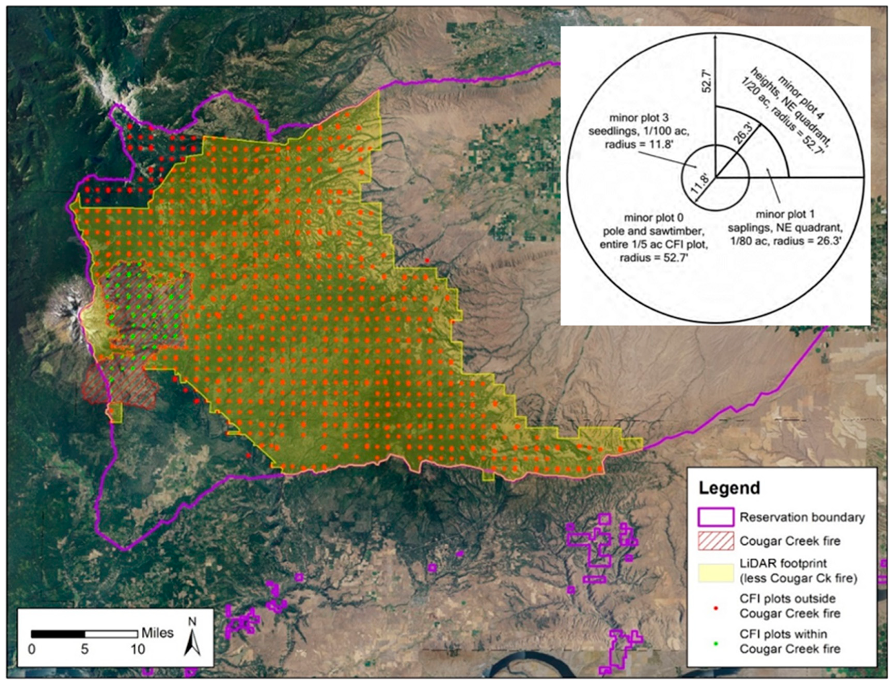
2.1. Study Area

This study was conducted on the forested lands of the YN, located in Washington State, US. The study area consists of 611,000 acres within a mixed conifer forest (Figure 1). The study area included the operational and non-operational forested acres within the reservation exhibiting multiple recent and past fire scars, harvest activities, and heterogenous structural conditions typical of a western United States (US) working forest. The landscape was dominated by a mix of conifer species including Douglas-fir (Pseudotsuga menziesii), ponderosa pine (Pinus ponderosa), lodgepole pine (Pinus contorta), western white pine (Pinus monticola), western redcedar (Thuja plicata), western larch (Larix occidentalis), grand fir (Abies grandis Engelmann spruce (Picea engelmannii), and whitebark pine (Pinus albicaulis). The local climate is characterized by cool and wet winters and warm and dry summers on the southern and eastern portions of the forested landscape at <3000 feet elevation, but cold snowy winters with mild and temperate summers in the northern and western areas around Mount Adams often >4000 feet elevation. As is standard in US forestry, data are reported in English units, with metric conversions provided in parentheses for clarity.

2.2. Forest Inventory Data

The CFI data acquisition process was defined by the Bureau of Indian Affairs (BIA) within the YN Forest Management Plan [12,27] specifications and occurred between 15 August 2015 and 29 November 2016. All CFI data for this study was directly provided by the YN for the specific purpose of this comparison and remains their sovereign data. Within the CFI, the landscape is divided into 1 mile by 1 mile (1609 m × 1609 m) grid squares, each of which contained 8 subplots. Each subplot is offset from the grid square by 40 m at 45-degrees azimuth and then 120 m more at 0-degrees azimuth. Subplots 1, 4, 5, 6, 7, and 8 are each offset from the corresponding grid square by 2 chains (40 m) at an angle of 45°. Subplot 2 is 6 chains (120 m) due north of the location of subplot 1, and subplot 3 is similarly 6 chains (120 m) due north of subplot 2. Although the BIA CFI design uses the terms plots and subplots, in this study we refer to each subplot as a “plot” given each is measured independently and is treated within the analysis as a single data point. Although the YN managed lands represent a larger area, the unfiltered CFI dataset provided for this assessment consisted of 1286 plots that the YN remeasured on a 10-year interval [12]. The CFI design presented in [12] originally called for measuring seedlings, saplings, and poles on some minor plots and not on others. In 2015, the YN amended the CFI collection, such that the following measurements were acquired across a series of minor plots (Figure 1):

-

DBH and all other tree data except for trees with a height of >5 inches DBH.

-

Data for all saplings between 1- and 4.9-inches DBH in 2-inch sizes classes.

-

Data for all seedlings between 1- and 4.5-feet tall and less than 1-inch DBH.

-

Height recorded for all trees greater than 5 inches DBH.

As the CFI experimental design illustrates, both DBH and total height were recorded on only minor plot 4 and only for trees with DBH greater than 5 inches, otherwise only DBH was recorded. Tree records for the CFI plots were expanded to a per-acre basis for input into the US Department of Agriculture and Forest Vegetation Simulator (FVS) system, given the sawtimber-size trees were sampled at a 1/5th acre (0.8 ha), sapling trees at 1/80th acre (50.5 m²), and seedlings at a 1/100th acre (40 m²).

2.3. Aerial LiDAR Scanning Data

ALS data were acquired in July 2019 using an Optech Galaxy Prime LiDAR sensor (Vaughan, ON, Canada) mounted in a fixed-wing aircraft. Elevation of the aircraft varied between 5000 and 9000 feet above ground level and flight lines alternated orientations while maintaining a 50% flight-line overlap following standard ALS forestry recommendations [28]. The average scan density was 16 ppm² with an average of 3 returns over the forested areas. The ALS data were preprocessed and classified as bare earth, vegetation, water, buildings, and noise returns by the vendor. The Optech Galaxy Prime scanner operates with a single oscillating mirror resulting in a zigzag or “sawtooth” laser path at the ground surface, which differs in data accuracy from the “matrix” pattern scanners that are more commonly applied in the western United States. Laser-pattern coverage is controlled at the ground surface for matrix scanners resulting in a more equidistant “grid” which has been shown to result in greater data consistency and improved results when processing [29,30,31]. Individual tree detection (ITD) within the ALS dataset was achieved using ForestView^® (Moscow, Idaho) [3,11,29,32,33], which provides a single-tree DI across a landscape and exhibits comparable or improved tree-detection accuracy compared to other common approaches [29]. The approach relies on classified ALS point cloud data and derivative datasets including high-resolution (0.3 m spatial resolution) digital elevation model and resultant similar spatial resolution canopy height models (CHM). Treetops are identified as localized peaks within the CHM and are identified using a combination of both CHM- and point-cloud-based individual tree detection methods in a similar manner to valley-following watershed segmentation and local max filtering that have been applied by numerous ALS individual tree detection studies [9,34,35,36,37]. A series of standard forest structural metrics such as height percentiles, stratified point densities, and crown shape derived from the point cloud for each detected tree are used to refine initial tree detections and derive other tree attribute information [11]. Individual tree DBH is modeled using these point cloud metrics, along with tree density, tree spacing, and additional allometric relationships derived from field-collected verification data [11]. Volume was derived in ForestView using DBH allometric relations, following the methods described in detail in [33]. In total the unfiltered DI produced 243,717 individual tree records subsequently allocated to 2.49-acre polygons across the study area.

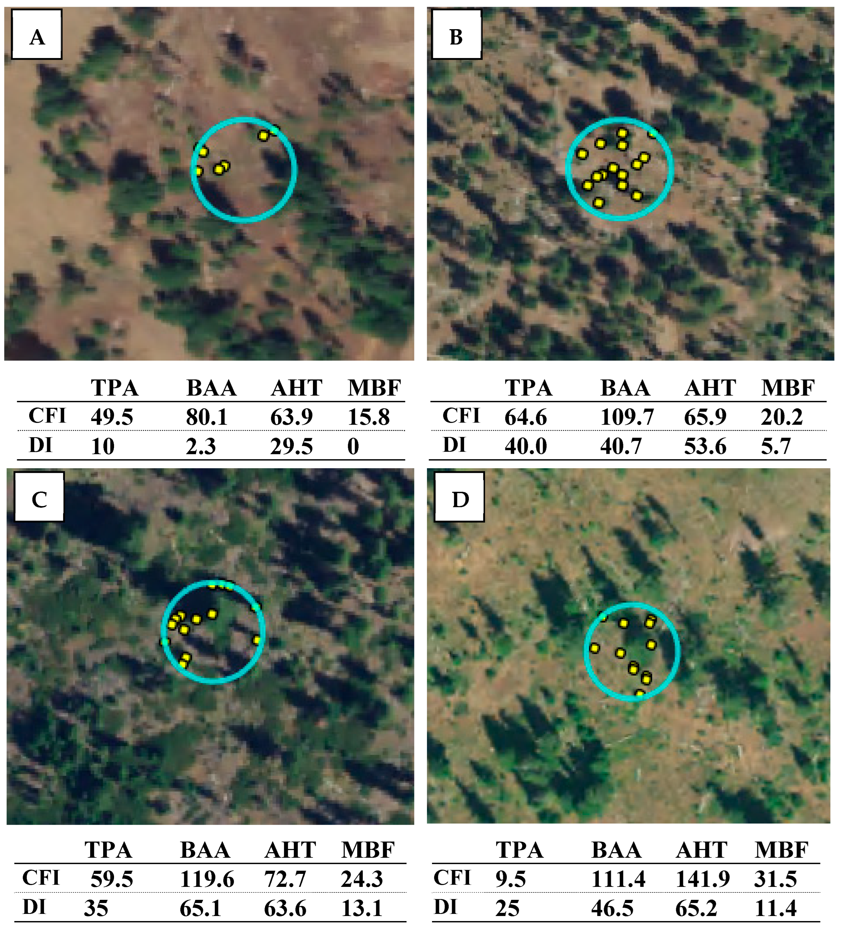
2.4. DI Field Validation Methodology

Although we acknowledge there is no feasible approach to retroactively evaluate the accuracy of the CFI data, given it was collected over multiple years and several years prior to the ALS acquisition and associated DI fieldwork, we were able to assess the relative accuracy of the DI method to an independent cruise dataset. However, we also acknowledge that the cruise data cannot be considered as ground truth data as it exhibits its own measurement errors that are often not reported, and as such this is only a relative comparison. As in [11,33], true ground truth data would include felled trees, where the maximum tree height can be accurately measured, without branches or other trees occluding the estimate. As we describe below, developing a DI using ForestView has been previously shown to exhibit lower bias and RMSEs of maximum tree height when compared to field cruise data, in which felled trees represented truth, on two very different forest types. Therefore, the ForestView DI is arguably an improved representation of the actual tree heights than the coincident cruise data. Consequently, we include this comparison as it may provide us insight into potential sources of uncertainty in the CFI data collection, given field methods to derive maximum tree height are broadly similar across studies.

To achieve the assessment, field validation data were collected in summer 2019, concurrently with the ALS dataset, to calculate statistical measures of accuracy and confidence associated with tree and stand metrics and DI. These field validation data were obtained by visiting 1029 randomly located field validation plots distributed throughout the 611,000 acres where sub-meter GPS points were monumented with a JAVAD Triumph-2 (JAVAD EMS, Silicon Valley, CA, USA), and measures of height and DBH were collected for each tree. Each location represented a standard ~65.6 foot (20 m) fixed radius “plot” where measurements of tree location, height, and crown were collected using a Vertex Laser Geo 360 hypsometer (HAGLOF, Langsele, Sweden). A diameter tape was used to measure DBH to the nearest 0.1 inch, and a Spiegel relaskop (SILVANUS, Kirchdorf, Austria) was used to gather a stem height, where 80% of DBH was used to approximate tree taper to inform volume calculations, given taper classes are usually based on the relative height where the upper diameter is 80% of the DBH. Following [33], we assessed the accuracy of the DI relative to the cruise data using regression-based equivalence tests [38]. Given the tree counts on the plot-level data differed, we assessed equivalence of maximum heights and total basal area per plot. Following [33,38], we report the minimum region of equivalence that rejects the null hypothesis of dissimilarity for both the slope and intercept. As in [33], the analysis was conducted in R [39] using the “equivalence” R Package version 0.8.1 [40].

2.5. Undisturbed and Geographically Aligned Plot Locations

Prior to the comparison of the CFI and ALS derived data, it was necessary to identify plots that had not experienced disturbances (fire, die off, harvesting, etc.) and that did not exhibit geolocation errors associated with data entry or GPS inaccuracies. We describe these two conditions as “undisturbed” and “aligned”. We define “undisturbed” as not exhibiting evidence of fire, harvest activity, or excess mortality between 2015 and the Digital Inventory^® data acquisition in 2019. “Aligned” was defined through multiple visual comparisons of the DI canopy height model images, satellite imagery, and National Agriculture Imagery Program (NAIP) imagery which provides 0.6 m spatial resolution imagery in the near-infrared, red, green, and blue spectra. The various datasets were spatially overlaid with each of the GPS locations provided in the CFI dataset, to determine if the reported CFI measurements were reasonable with the imagery. Initially, 66 CFI plots were either located outside the ALS acquisition area or had no LiDAR coverage. Another 18 had either no coordinates or were assigned incorrect coordinates that duplicated those of another plot. Within the study area, only a single wildfire was recorded over the analysis period. Namely, the August/September 2015 Cougar Creek Fire that burned roughly 41,500 acres within the study area. Consequently, 100 plots were excluded as they either fell within the fire perimeter or were close enough to the perimeter to have sustained damage. Finally, 24 plots were excluded because comparison of 2015- and 2019-vintage NAIP imagery indicated that partial harvest occurred sometime between 2015 and 2019. This process left an intermediate set of 1078 potential plots. However, clear outliers were observed in VPA and therefore 11 CFI plots that exceeded the 99th percentile of VPA were excluded in the analysis. This left 1067 plots for comparative analysis.

2.6. Forward Growth Modeling

To compare the CFI to the ALS-derived DI, the individual digital-tree records probabilistically occurring within the boundary of each CFI plot were determined by drawing a one-fifth acre (52.7-foot radius) circle around each CFI plot center and using the ESRI ArcGIS Pro version 10.1 spatial join tool to select DI tree records within each plot boundary. CFI and DI data were matched by GPS coordinates of the tree list data within each stand and CFI data were then input to FVS to forward model the CFI data to the date of the DI and compute various stocking estimates such as BAA and VPA. The East Cascades variant was used in this analysis to best approximate local forest conditions during modeling, where necessary parameters for FVS were derived from the CFI database. The East Cascade variant of FVS uses, by default, 7 inches as minimum DBH for sawtimber volume; hence any 5- and 6-inch DBH trees have no sawtimber volumes assigned.

To verify that CFI data were correctly input to FVS, the initial plot-level BAA computed by FVS in trees ≥5 inches (0.127 m) DBH was compared with the values presented in the CFI database. For all sample plots, the FVS-reported BAA was within ±0.05 sq ft ac⁻¹ (0.011 sq m ha⁻¹) of that reported in the CFI database, with 55% of the plots being statistically similar (92% within ±0.01 sq ft ac⁻¹ (0.002 sq m ha⁻¹)). This confirmed the FVS model computations were consistent with the CFI processing methodology. CFI data on the 1067 plots were then grown in FVS to 1 January 2020, given the DI was acquired after most of the 2019 growing season (and hence tree-growth) had already occurred. Again, following [33], we assessed the statistical equivalent of the DI to the forward-modeled CFI data using regression-based equivalence tests [38]. As with the DI validation we assessed equivalence of maximum heights and total basal area per stand. Following [33,38], we report the minimum region of equivalence that rejects the null hypothesis of dissimilarity for both the slope and intercept. As in [33], the analysis was conducted in R [39] using the “equivalence” R Package [40].

2.7. Reassessing Alignment Following Forward Modeling Using Aerial Photography

Following the processing of the forward modeling, we observed that several plots still exhibited considerable differences in maximum heights and BAA between the CFI and DI that could not be explained by DI missing small, co-dominant, or suppressed trees. To address the observed BAA differences, we flagged any plots with BAA differences of greater than 50 sq ft ac⁻¹ for analysis. Under this criterion we evaluated 2015 and 2019 NAIP imagery and identified 2 plots near the delineated Cougar Creek fire burn perimeter that exhibited excessive mortality and 24 plots where partial harvest activity occurred between CFI and LiDAR data collection. While this analysis addressed the BAA differences, it provided few insights to explain the occasions of notable differences in total tree heights. As shown in Figure 2, it was readily apparent when viewing NAIP aerial imagery that several DI and CFI plot center locations remained misaligned, i.e., the GPS locations recorded for those plots were not accurately determined relative to the actual CFI plot center. As the examples in Figure 2 illustrate, there are clear shadows from large trees outside of each plot that have likely been incorrectly included by the CFI measurements.

To address this issue, the second filtering methodology consisted of two steps:

(1)

Assessing the difference in height of the tallest tree on each CFI plot (measured or imputed) versus the tallest tree as estimated on each corresponding DI plot.

(2)

Assessing the number of trees per acre of the tallest trees on a plot.

In this analysis, we assessed the 2015 and 2019 NAIP imagery for each geolocated LiDAR-derived plot center location, which had been determined with a high degree of accuracy to identify CFI plots with clear positional errors that could not be readily corrected by dithering the plot center location by a few meters. To achieve this, we took the CFI plot GPS coordinates as given and assumed no significant vegetative changes had occurred. In theory, the tallest trees should be roughly the same in both the DI plots and forward-modeled CFI plots. However, given tree heights were only collected for a small sample of the CFI trees, the tallest tree on the CFI plot may not have height measurements. We therefore assumed a CFI to DI maximum tree height difference would still identify plot locations of interest for filtering. We also assumed that the tallest trees within both datasets are defined as trees greater than or equal to the ratio of 90% of the tallest tree on each plot, i.e., if the tallest tree on a plot is 100 feet (30.48 m), the 0.9 height ratio class (HTRC) would consist of all trees at least 90 feet (27 m) tall. Therefore, if the CFI and DI are considering the same ground location, the TPA represented by the tallest trees (i.e., 0.9 HTRC) in a plot should not vary considerably. The use of HTRC allows the analysis of strata defined by tree heights alone rather than using percentiles of tree heights, which would include the effects of both tree heights and TPA. To limit the potential of either the CFI or DI to skew results due to use of arbitrary height breaks, we limited the cross-comparison to plots where (i) the tallest DI tree height was within ±11.8 ft (3.6 m) of the tallest forward modeled CFI tree height and (ii) the difference in TPA between the CFI and DI datasets represented by the 0.9 HTRC was within 39.9 trees ac⁻¹ (98.5 trees ha⁻¹). We then further compared the forward-modeled CFI with the DI, which revealed additional disparities between the tree distributions at the plot level, indicating that these plots were likely unaligned. This resulted in filtering an additional 466 plots out of 1067, leaving 601 plots for in-depth analysis.

2.8. Direct CFI and DI Comparison

We examined the relationship between CFI and DI measurements using the 1067 and 601 available plots by comparing tree heights, TPA, BA (per tree and per plot), BAA, and gross VPA. To achieve this, we used FVS to grow the CFI data to the same date as the data acquired by LiDAR in 2019. The absolute differences between matched CFI and DI plot locations were computed as the DI result minus the CFI result. This statistic describes whether the differences observed are significantly different from zero and thus meaningful regarding one dataset providing a view that varies relative to the other for specific attributes.

2.9. CFI Sample-Based vs. Population-Based Forest-Wide Comparison

The preceding sections described methodologies employed for plot-to-plot comparisons between the CFI and DI inventories. A further analysis was conducted involving a comparison of the CFI and DI on the total ~611,000 acres of operable forestlands within the YN. For this forest-wide analysis, no adjustments were made for harvesting or forest growth; although we acknowledge that this introduces some potential differences, we assumed harvest and growth were well-balanced across the entire forest during the period 2015 to 2019. Further, this approach avoids any variance that might occur due to growth-model effects at a landscape scale. While such considerations are critical when performing a plot-by-plot comparison, adjusting for them is less critical in a forest-wide comparison. Additionally, the Cougar Creek fire occurred before CFI in-field remeasurement so, both the CFI and the DI were considered an accurate reflection of conditions within and near the wildfire perimeter at the time of their respective measurements. For these reasons, the Cougar Creek CFI points were included in this forest-wide analysis. Excluding CFI plots that fell outside the DI collection footprint resulted in 1210 plots. These 1210 plots were treated as a simple random sample and processed through the FVS model to compute inventory values. The DI coverage overlapped the CFI dataset on 586,414 acres meaning our expansion factor for each of the 1210 CFI plots was assumed to be 484.6396 acres per plot to accurately represent the total forested area.

3. Results

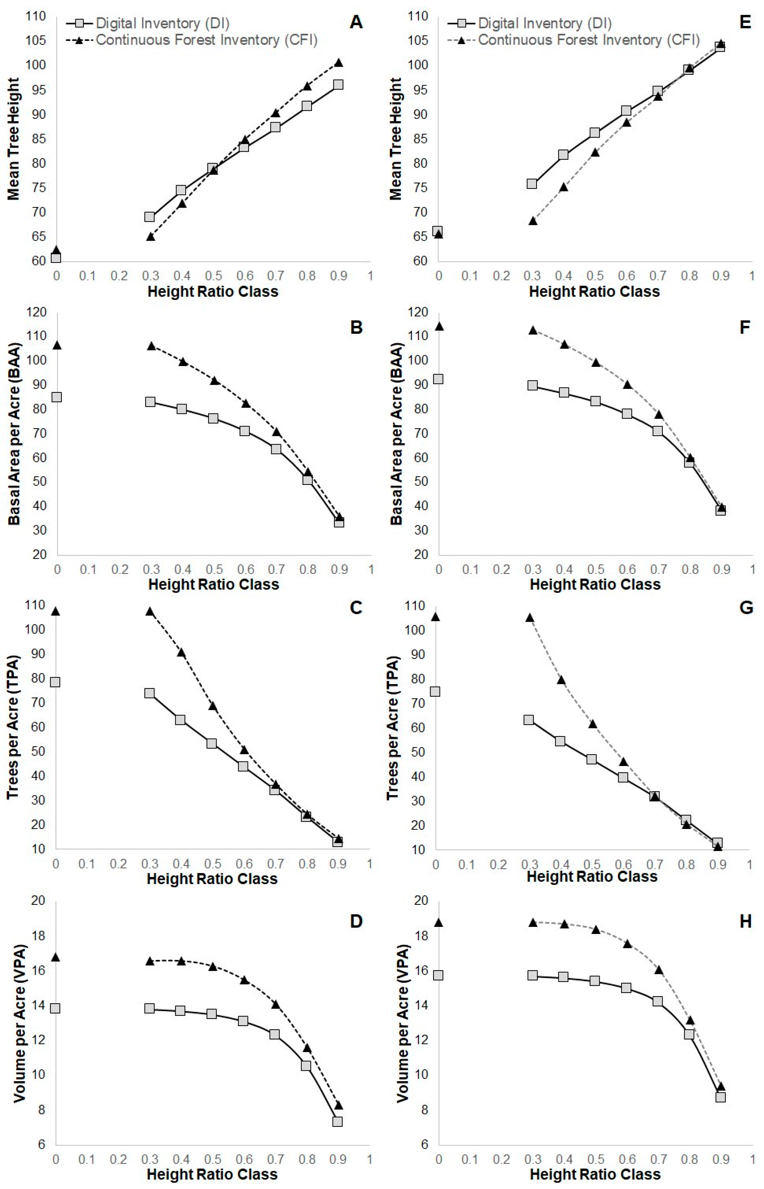
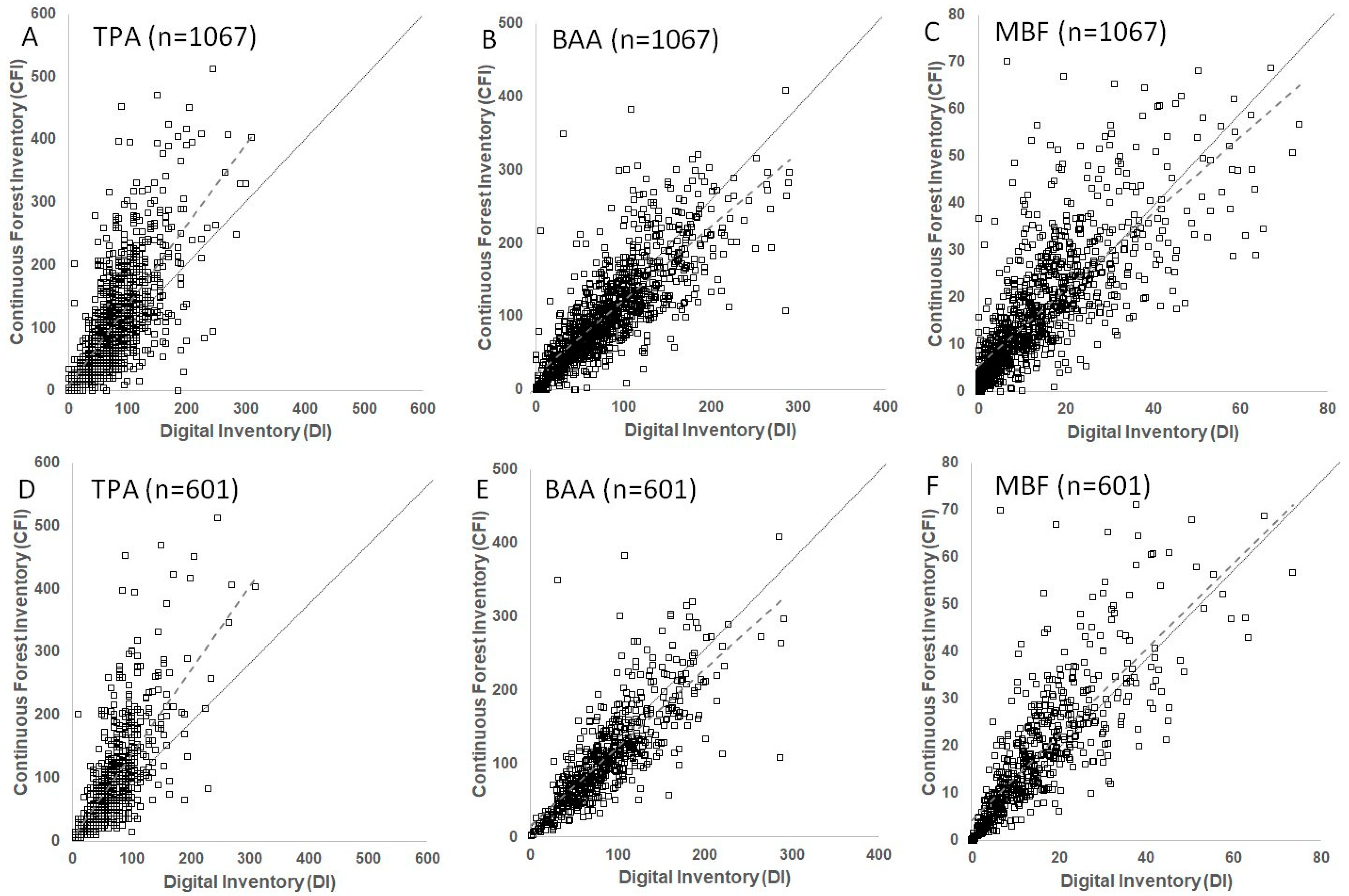
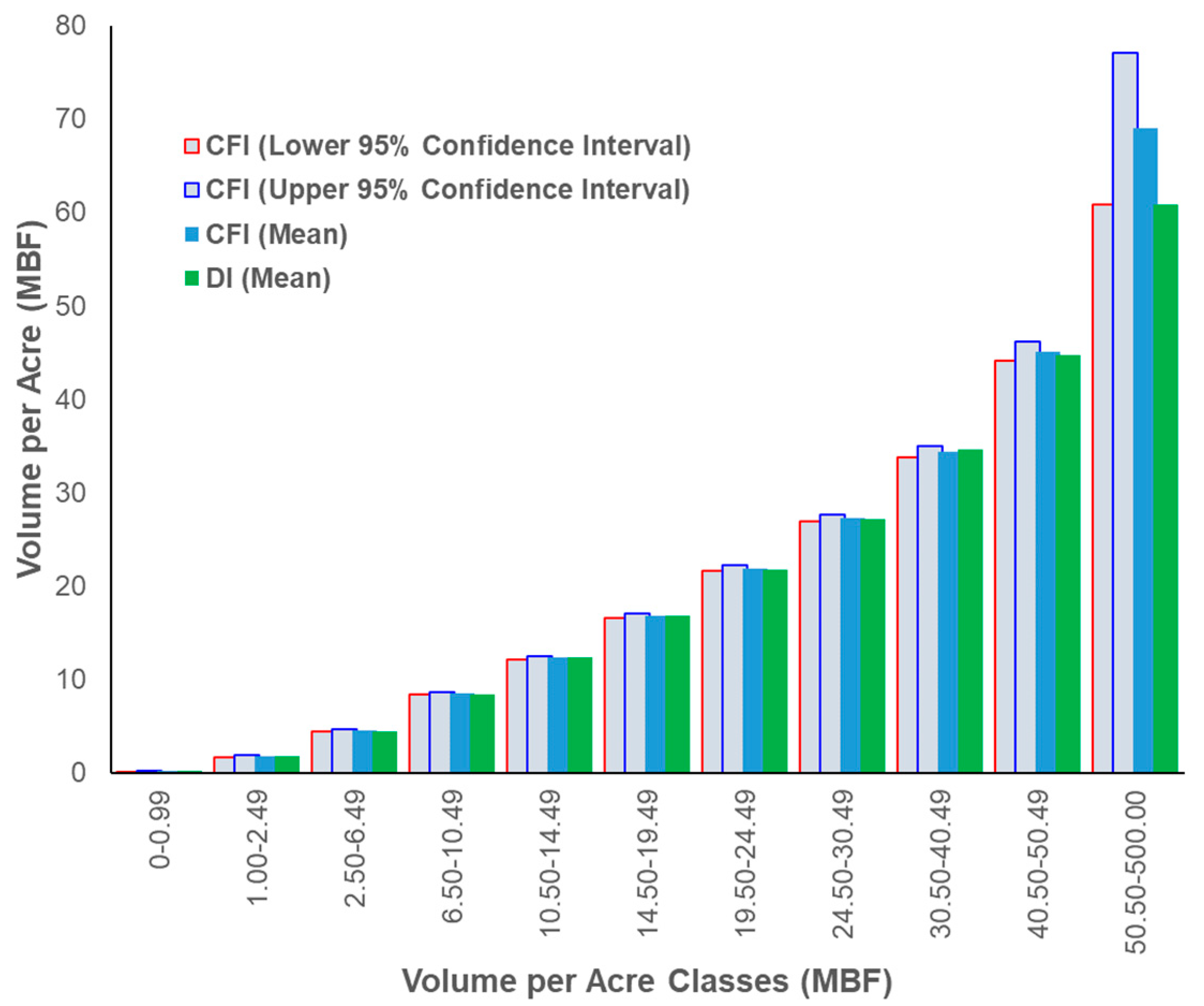
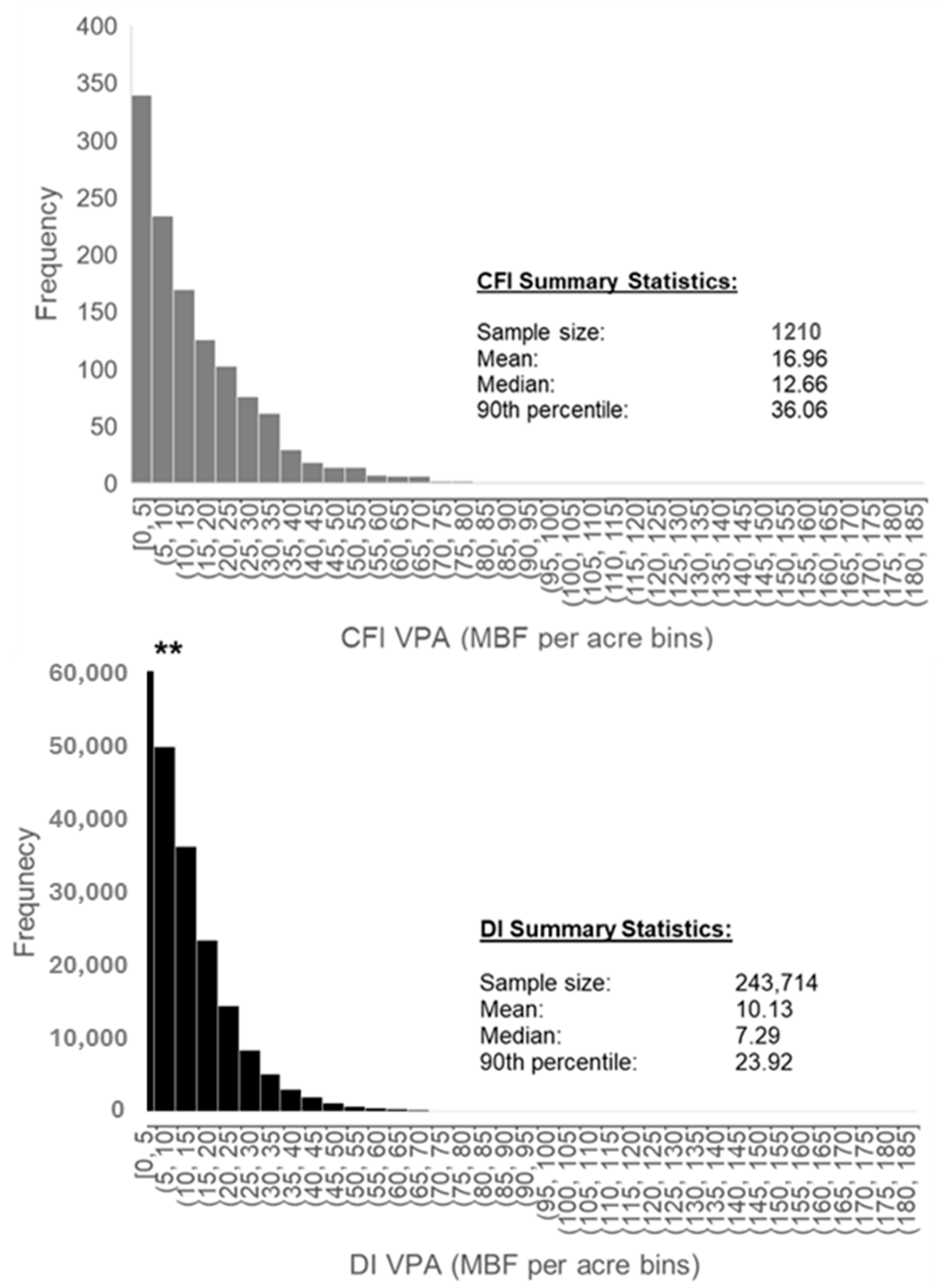
3.1. Comparison of Forward-Modeled CFI to DI (Plot-to-Plot Analysis)

The DI and CFI estimates of trees per acre (TPA), basal area per acre (BAA, sq ft ac⁻¹), and volume per acre (VPA, thousand board feet per acre, MBF ac⁻¹) were graphed for the initial (1067 plots) and secondary (601 plots) filtered data (Figure 3A–F). The initial filtering approach produced 1078 plots. However, clear outliers were observed in VPA and, therefore, the 11 CFI plots that exceeded the 99th percentile of VPA were excluded in the analysis. This left 1067 plots that are shown in Figure 4A–C and 601 plots shown in Figure 4D–F.

The comparison of TPA for CFI and DI across the 1067 plots (Figure 4A) shows that relative to DI, higher tree counts were observed on the CFI plots (gradient: 0.38). When comparing BAA (Figure 4B) relative to DI, the BAA on the CFI plots was slightly higher (gradient: 0.63) and the estimates of VPA (Figure 4C) showed reasonable correspondence between the DI and CFI (gradient: 0.73). For the analysis of the 601 plots following the second set of filtering, the comparisons (Figure 4D) show that relative to DI, there remains a tendency toward higher TPA (gradient: 0.34), higher BAA (gradient: 0.60), and marginally higher VPA (gradient: 0.68) on CFI plots. When considering the 1067 plots, the median TPA in the CFI plots was 665 and the median TPA in the DI plots was 105. For BAA, 23 CFI plots exceeded 300 sq ft ac⁻¹, whereas the maximum reported DI BAA across all 1067 plots was 291 sq ft ac⁻¹. In the 1067 plots, there were 9 plots in which the DI indicated ≥60 MBF ac⁻¹ versus 10 plots in the CFI data with ≥60 MBF ac⁻¹ (≥57.27 m³ ha⁻¹).

Whether considering the 1067 or 601 plots, BAA becomes not significantly different (α = 0.05) at the 0.8 HTRC, whereas average tree height is not significantly different only when including all trees ≥5-inches DBH. As shown in Figure 3, as the HTRC exceeds 70% of total tree height, the DI and CFI estimates of TPA, BAA, and VPA generally converge, with Figure 3A representing the only exception. Overall, this suggests the DI and CFI data are generating similar results for the largest and arguably most valuable portion of the forested resource. Overall, the CFI VPA was 18% higher than the DI average for all trees ≥5-inches DBH. The average tree height between the CFI and DI datasets was not statistically different for all trees ≥5-inch DBH, which is consistent with prior LiDAR height studies [8,41]. TPA was statistically different when comparing the CFI and DI datasets for all trees ≥5-inch DBH. BAA between the DI and CFI datasets were not significantly different in the 0.9 and 0.8 HTRCs. When considering the comparison of the 1067 to the 601 plots with respect to BAA and VPA, the variance visually declines with the lower sample size with notable increases in the r², supporting the rationale to reduce the plots to 601 plots.

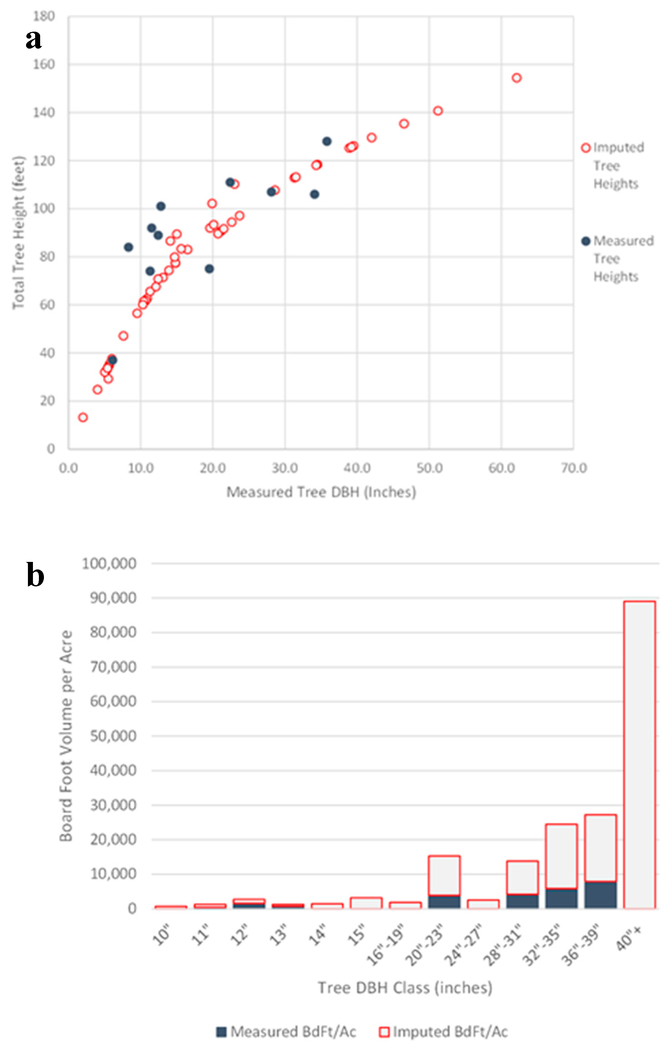
3.2. DI Field Validation Results

The distributions for tree height and basal area per tree in the field validation cruise and the DI are shown in Figure 5a and Figure 5b, respectively. In each case the distributions were similar, except that as expected the DI identified fewer trees than the field cruise. The regression-based equivalence tests for cruised maximum heights and total basal area on the plots versus the DI maximum heights are shown in Figure 6a and Figure 6b, respectively. The intercept values for the cruised versus DI maximum height and total basal area were equivalent at a region of equivalence of ±3% and ±31% or greater, respectively. The slope values for the cruised versus DI maximum height and total basal area were equivalent at a region of equivalence of ±9% and ±12% or greater, respectively. The linear relationship between the cruised and DI maximum height had a strong r² of 0.9 (p < 0.001), while the linear relationship between the cruised and DI total basal area still had a reasonably strong r² of 0.78 (p < 0.001).

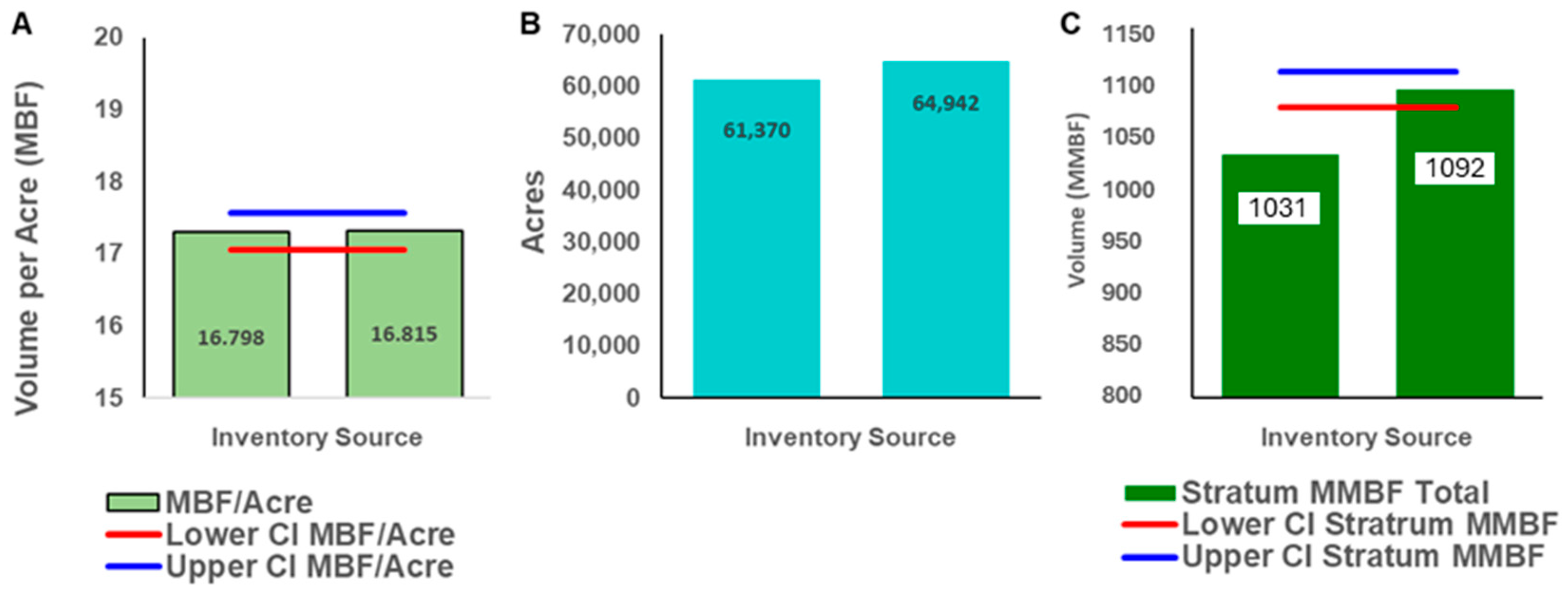
3.3. CFI Versus DI Landscape Estimate

Within the forest-wide comparison, the CFI contained data from 1210 plots consisting of data from ~30,000 trees whereas the DI contained 243,714 2.49-acre polygons containing ~40.4 million LiDAR point cloud samples representing relative elevations of trees. Figure 7A displays VPA and acres of the two inventories, by stand density class. When separated in this way stand density is defined on a BAA basis. While the total forest inventory is an important benchmark, total forest inventories as a single aggregate value are rarely used by forest managers. When comparing the results of the two measurements by BA class, the DI reflects a forest with more acres in the lower stand density classes and generally higher VPA than the CFI for each corresponding stand density class. Figure 7B breaks down the two inventories by both VPA and acres by tree class. The size class for this assessment was defined by the quadratic mean diameter (QMD) output from FVS. When comparing the results of the two inventories in this way, the DI displays a forest with more acres in larger size classes than the CFI for the same size class. In addition, the DI volumes per acre show a much smoother progression of VPA by size class than is seen for comparable size classes of the CFI. We postulate that this outcome is partly attributable to the result seen in the plot-by-plot comparison where the DI tends to underreport small trees resulting in a larger average tree size. Figure 7C illustrates a comparison of the inventories on cumulative forest-wide volume and acres basis by VPA classes. When comparing the results of the two measurements cumulatively by VPA class, there is reasonably close correspondence between the DI and CFI until the 19.5 MBF ac⁻¹ (18.6 m³ ha⁻¹) and greater classes. The DI generally has greater acreage by volume class until 19.5 MBF and then the situation is reversed, with CFI having greater acreages for classes greater than 19.5 MBF.

The regression-based equivalence tests for CFI maximum heights and total basal area on the plots versus the DI maximum heights are shown in Figure 8a and Figure 8b, respectively. The intercept values for the CFI versus DI maximum height and total basal area were equivalent at a region of equivalence of ±16% and ±33% or greater, respectively. The slope values for the CFI versus DI maximum height and total basal area were equivalent at a region of equivalence of ±19% and ±42% or greater, respectively.

Figure 9 compares the average CFI and DI VPA by volume-per-acre class, along with lower and upper bounds of the CFI’s 95% confidence interval. As can be seen, there is a close correspondence between the two measurements by volume class until the largest class when the DI estimate falls outside (specifically, below) the CFI’s 95% CI. Figure 10 illustrates the results when considering a single VPA stratum (14.5–19.499 MBF/acre). Despite the CFI and DI volumes/ac and acres being well aligned, when the per-acre estimates are expanded to a class total and the corresponding confidence intervals applied, the CFI confidence interval no longer includes the DI total (Figure 10). This demonstrates how small acreage-class differences can exert significant impacts on forest inventory estimates. It also highlights an often-underappreciated aspect of a DI: whereas a traditional inventory estimates volume per acre of strata, a DI can provide a unique volume estimate for every acre of the forest. As noted, the 1210 CFI plots in this study each represent only 0.2 acres (i.e., size of the fixed-radius CFI plot) or the conditions on ~242 acres (~0.04%) out of the total 586,414 forested acres included in the DI. Therefore, the DI provides geolocated information on the conditions within the other 99.96% of the acres.

4. Discussion

4.1. Location Uncertainties

The ability of the DI to generate location coordinates for each sampled tree made it possible to readily identify the DI trees within each CFI plot radius; however, the accuracy of this process relies on the accuracy of the CFI plot location data. If CFI plot locations are inaccurate the DI tree records selected for that CFI plot will have a lower likelihood of accurately representing the CFI plot. The CFI also has spatial errors associated with the GPS, processing, and georeferencing, which further compounds uncertainty associated with matching the DI to the CFI or field validation datasets. Ideally, future studies would not rely on the provided GPS locations; instead, each CFI plot would be revisited, and locations recorded using high-precision GPS equipment. However, such a re-assessment would likely be time and cost prohibitive. GPS inaccuracies can occur for multiple reasons, such as malfunctioning GPS receivers, data entry errors associated with coordinates being improperly recorded, poor GPS reception at the plot location due to older technologies or high canopy cover, time allocated for GPS signal stabilization, and/or mismatched GPS coordinate systems [42,43].

Generally, the DI results for TPA and BA are significantly different from the CFI data for the four metrics examined in the plot-to-plot analysis: average tree height (ATH), BAA, TPA, and VPA (volume measured as Scribner board foot volume). The results for comparison of TPA, BAA, ATH, and VPA demonstrate that the CFI generally reflects higher, sometimes substantially higher, plot TPA, BAA, and VPA than the DI when limited to our comparison of trees ≥5 inches DBH. This limitation was applied because LiDAR scans are known to miss understory and occluded (i.e., intermediate and suppressed) trees [44]; we contend that the CFI measurements for <5-inch DBH would be the most reliable. Although the DI undercounts these smaller trees, they represent only a small fraction of the merchantable timber (Figure 3).

4.2. Tree Heights

Tree height measurements from the DI, for the tallest trees within the dataset, averaged 1.1 feet (0.33 m) less than the modeled heights from the CFI data. These results are consistent with other studies and can occur for a number or reasons, such as the LiDAR data not ‘hitting’ the leader, occlusion by other treetops or branches, and instrument parameters such as signal reset time and scanning pattern, among others [41]. Research comparing the vertical accuracy of numerous LiDAR scanners suggests greater accuracy can be achieved when densities exceed 10 pulses per square meter [45,46,47]. Conversely, the difference in heights could be the result of measurement errors propagated from the forward modeling of tree heights, as research on forest growth projections has shown some models can overpredict tree height [48] and volume [49] when data does not capture field variability [50]. However, the short time interval of the forward modeling (i.e., <4 years) likely minimized this source of error. Another source of potential error is due to CFI data often not being available until multiple years following field collection [51], which could potentially amplify data entry errors due to a lack of familiarity with the measured plots as well as potentially not accurately representing the current landscape as well as the potential influences of a changing climate or precipitation conditions [52].

4.3. Trees and Volume per Acre

The differences in TPA for regeneration-sized trees between the CFI and DI data are an important aspect of this research and draws attention to the scanning pattern of the LiDAR sensor used in this study. Contemporary sensors with matrix scanning patterns [53] are considered the industry standard as of 2020 and offer greater spatial accuracies with increased pulse densities [30,31]. This enables processing for vegetative objects viewable from the air down to a height of <6 feet (1.82 m) in many ecosystems. In addition, other improved techniques provide for better detection and imputation of smaller trees, even those beneath the taller forest canopy. Despite the divergence between CFI and DI for the shorter trees on a plot, Figure 3 shows that for most of the volume, the two measurements are in reasonable correspondence. The difference between VPA for the two methodologies on the forest-wide basis shows good correspondence up through the 19.5–24.488 MBF ac⁻¹ volume class (Figure 7C). For this class, the VPA is not statistically different between the CFI and DI; the acres are comparatively close, and yet when the confidence intervals are computed on a total inventory basis for the class, the CFI and DI in this class are significantly different (p < 0.05). Often, attention is focused on tree volume, with relatively little attention focused on acres. As illustrated in this study, the DI is a population estimate while the CFI is a sample-based estimate, meaning each plot of the CFI is intended to represent a specific number of acres for a certain condition. In this study, each plot represents 484.6397 acres, and the total 1210 plots are reporting conditions on 242 acres (0.04%) of the total 586,414 acres, whereas the DI is reporting conditions on all 586,414 acres.

We acknowledge that this misalignment could potentially be due to multiple factors such as previously unidentified non-fire disturbances, such as windthrow, insect or disease-based mortality, density, and age-based mortality, unaccounted for ingrowth since the CFI assessments, or the DI method missing some number of co-dominant or overtopped trees. However, given the NAIP assessment, we believe the more plausible explanation is that this uncertainty occurred due to malfunctioning GPS receivers and/or coordinates being improperly recorded, poor GPS reception at the plot location, use of older GPS units with poor resolution, time allocated for GPS signal stabilization, whether real-time or post-processed GPS corrections were applied, and mismatched GPS coordinate systems, among other sources of uncertainty. We also postulate that it is feasible the CFI plot coordinates were initially collected to provide general plot locations that would assist field crews in navigating the plots, and thus coordinates did not need to be highly precise. Although some might argue that this second level of filtering could bias the results towards the DI, the converse (i.e., retaining the 466 plots) would potentially bias the results towards the CFI. The second filtering was conducted to ideally limit potential bias by focusing on plots where there was confidence that the GPS data were reliable and that the CFI and DI were considering the same areas, thus mitigating a potential source of variability due to lack of precision with respect to common plot location.

4.4. CFI Sources of Error

We observed an unexpectedly high degree of departure from the plot layout specified by the 2005 CFI field manual. In addition, there were disparities in the number of plots measured in the CFI. Notably, in 199 plots, the tallest DI tree was shorter than the tallest CFI tree, while in 93 plots, the scenario was reversed. An additional potential source of uncertainty in CFI is that once selected to be permanent measurement plots, trees are not treated in the same way as the rest of the forest. Consequently, the monumented observations are not representative of the population. This contrasts with the DI, which captures information across the entire variation in conditions across the forest. Figure 11 shows the comparison in distributions and statistics between CFI and DI for VPA for the entire forest (i.e., unfiltered data). This figure best illustrates that DI is effectively a population level estimate as the data are derived from the 243,714 2.49-acre polygons in which all detected trees are assessed, whereas the CFI represents 1210 plots from which only a small partition of tree heights are measured (Figure 1).

As Figure 11 shows, the general shape of each histogram is very similar, with data achieving an asymptote in each case around the 65 MBF per acre bin. A comparison of the medians yields comparable results, and each distribution is similarly positively skewed. Given medians are less sensitive to extreme values than averages, even if several plots have been treated differently, the median will still provide a measure for the central point of the population and provide a more reasonable comparison. The occurrence of high-volume outlier plots within the CFI data are illustrated by the distribution exhibiting a high positive skew with the 90th percentile of the CFI VPA data being at 32.953 MBF ac⁻¹, while the maximum is 184.7 MBF ac⁻¹, as compared to the DI 90th percentile of 23.92 MBF ac⁻¹ and a maximum of 127 MBF ac⁻¹.

Furthermore, during the plot-to-plot analysis, 11 CFI plots were removed, given they exceeded the 99th percentile of VPA, but these plots remained within the forest-wide analysis. Figure 12 illustrates the impact of including these plots. Figure 12a shows the actual height versus predicted height measurements for the plot at the most extreme end of the VPA distribution. As can be seen, the upper end of the heights was predicted to increase in a near linear manner, while a more compressed sigmoidal curve or asymptote would usually be expected. Figure 12b shows the impact of this by illustrating the difference between the trees where measurements of both DBH and height existed to create the volumes versus the imputed volumes. As can be clearly seen, the imputed volumes considerably inflate the inferred volume to extreme values.

This outcome suggests that, on a VPA basis, the results between DI and CFI are potentially only different because of plots at the upper end of the VPA distribution which provides support for exclusion of these plots from the plot-to-plot analysis. While such high-volume conditions may exist in the forest, they exist in isolation, and probably not to the degree that the standard plot-expansion factor may suggest. Although additional research is necessary to explore this phenomenon [54,55,56], it however does suggest that while the DI is delivering reliable VPA, perhaps the greatest value it provides is insight into the distribution and extent of forest conditions across the entire forest as opposed to traditional sample-based distributions of conditions associated with the CFI.

4.5. DI Accuracy Assessment

We showed that the DI measures of maximum height were statistically equivalent to the field validation cruise measurements at regions of equivalence of ±3% or greater for the intercept and ±9% or greater for the slope. These strongly equivalent results concur with past studies that have assessed the effectiveness of the ForestView approach to create a tree height DI. Notably, in a comparison of the ForestView DI to both a cruise and independent felled-tree validation in a loblolly pine stand in Eastern Texas, ref. [11] demonstrated that the detection accuracy of ForestView was 97.1% and that the DI was an improvement over the traditional cruise heights when compared to the felled tree data. Specifically, the DI derived from Forestview exhibited a lower bias and RMSE for height than the traditional cruise-based inventory [11]. A similar cross-comparison was conducted by [33] on a mixed conifer forest in northern Idaho, where a ForestView DI was compared with a traditional cruise and log-scaling data. In that study, although the heights derived from the DI were statistically equivalent to the traditional cruise data, the DI exhibited lower height RMSEs and bias [33]. Furthermore, ref. [33] documented that although the DI under-detected some trees in the current study, it nevertheless accounted for up to 99% of the merchantable volume as measured at the mill.

We also showed the DI measures of total basal area per plot were statistically equivalent to the field validation cruise measurements at regions of equivalence of ±31% or greater for the intercept and ±12% or greater for the slope. These results again illustrate that the DI does underestimate the basal area. However, Figure 5a,b show that at the upper end of both the height and basal area distributions, the DI and field validation data were broadly similar, implying that for these 1029 plots, the DI is not missing large trees that would account for a major proportion of the basal area or volume in the plots. This result is notable as Figure 11 demonstrates that the DI and CFI forest-wide distributions of VPA were broadly similar, except that the DI appeared to exclude some very high VPA plots occurring at the far-right hand side of the distribution. The lack of similar omissions in the direct comparison of the DI and field validation data raises questions about the accuracy of these very high VPA values within the CFI.

When considered with these two similar previous studies, the data in the current study provides further evidence that the DI likely represents an improved estimate of the forest condition as compared to the sub-sample-based traditional cruise approach of CFI, and that differences between the DI and CFI inventories do not necessarily reflect deficiencies in the DI approach.

5. Conclusions

To recap, the research questions of this study were:

• How effectively does the DI capture regional inventory information, such as heights, TPA, BAA, and VPA, when compared to forward-modeled CFI data?
• What sizes of trees are the DI- and CFI-derived inventories effective at describing?
• What are the sources of uncertainty in the base CFI, forward-modeled CFI, and ALS-derived inventories?

When considering a direct comparison of CFI and DI in the absence of validation data concurrent with when each dataset was acquired (i.e., 2015 and 2016 for CFI, and 2019 for the DI), the observed differences between CFI and DI could be dismissed as simply DI missing small trees, where such a conclusion assumes that the CFI represents ground truth data. As we showed in the DI versus field cruise data, the DI clearly misses some trees, but importantly not at the upper end of the observed size classes. Even though the DI is not a complete census, it is likely closer to a population estimate as every tree across all size classes that is detected has its height and other attributes measured. In contrast, within each CFI plot, only a small percentage of trees greater than 5 inches DBH have their heights measured. Consequently, the CFI data cannot reasonably be considered ground truth data, and the direct comparison alone cannot be used to infer which of CFI or DI is the more accurate dataset. Furthermore, when considering the DI validation dataset within this study with the DI validation studies, to date, that cross-compared DI and field cruise data with ground-truth felled trees, the DI should arguably be considered the more accurate dataset as compared to CFI. Furthermore, unlike CFI, the uncertainty within the DI estimates is known, given they have been validated in this study and in prior studies.

An additional source of uncertainty associated with CFI is that trees are often not treated in the same way as the rest of the forest. Consequently, the monumented observations might not be truly representative of the population. This contrasts with the DI, which by design captures information throughout the entire variation in current conditions across the forest. Furthermore, additional CFI volume errors may arise through the use of FVS given FVS by default sets a minimum DBH for sawtimber at 7 inches, meaning that any 5- to 6-inch trees will be set to have zero MBF volumes [57].

For the total forest-wide (landscape) analysis, the CFI was 44% higher than the DI for volume. However, the analyses suggested this difference could be at least partially attributed to on-plot bias due to very high VPA plots within the CFI data (i.e., Figure 12). Consequently, forest management may want to consider including DI-based inventories when making planning decisions. Importantly, we contend that both CFI and LiDAR datasets such as DI are essential for effective forest management. CFI datasets allow forest management to monitor long term impacts on forested ecosystems, including quantifying the impacts of fires, insects, windthrow, etc. CFI datasets also include assessments of saplings and defects, each essential to future growth and yield predictions. In turn, DI-based datasets provide large-scale data of all trees across management areas. DI-based datasets can be used to diagnose potential problems in CFI and other field inventory datasets, such as inaccurate GPS locations, missing or adding trees, or data entry errors. Furthermore, DI-based inventories can provide data in the gaps where CFI has no data due to standard buffers such as near riparian zones or roads, or in remote inaccessible areas. LiDAR acquisitions are also associated with considerable value-added datasets, such as digital elevation models, information on slope stability, forested roads and trails, habitat data, riparian areas, and fuels and fire risk, among many others [5,58,59].

This study has concentrated on comparing the inventories of a sample-based measurement, the CFI, to a population-based measurement, the DI. The analysis demonstrated that although DI is missing smaller trees compared to CFI’s sample-based estimate, the value of a complete-coverage DI to describe the extent and distribution of forested conditions across a forested landscape cannot be overstated; when used together CFI and DI datasets represent a powerful set of tools within the forest management toolkit.

References

1. Falkowski, M.J.; Smith, A.M.S.; Hudak, A.T.; Gessler, P.E.; Vierling, L.A.; Crookston, N.L. Automated estimation of individual conifer tree height and crown diameter via Two-dimensional spatial wavelet analysis of LiDAR data. Can. J. Remote Sens. 2006, 32, 153–161. [Google Scholar] [CrossRef]
2. Hudak, A.T.; Strand, E.K.; Vierling, L.A.; Byrne, J.C.; Eitel, J.U.H.; Martinuzzi, S.; Falkowski, M.J. Quantifying aboveground forest carbon pools and fluxes from repeat LiDAR surveys. Remote Sens. Environ. 2012, 123, 25–40. [Google Scholar] [CrossRef]
3. Sparks, A.M.; Smith, A.M.S. Accuracy of a LiDAR-based individual tree detection and attribute measurement algorithm developed to inform forest products supply chain and resource management. Forests 2022, 13, 3. [Google Scholar] [CrossRef]
4. Nelson, R.; Parker, G.; Hom, M. A Portable Airborne Laser System for Forest Inventory. Photogramm. Eng. Remote Sens. 2003, 69, 267–273. [Google Scholar] [CrossRef]
5. Hudak, A.T.; Evans, J.S.; Smith, A.M.S. Review: LiDAR Utility for Natural Resource Managers. Remote Sens. 2009, 1, 934–951. [Google Scholar] [CrossRef]
6. Wulder, M.A.; White, J.C.; Nelson, R.F.; Næsset, E.; Orka, H.O.; Coops, N.C.; Hilker, T.; Bater, C.W.; Gobakken, T. LiDAR sampling for large-area forest characterization: A review. Remote Sens. Environ. 2012, 121, 196–209. [Google Scholar] [CrossRef]
7. Falkowski, M.J.; Hudak, A.T.; Crookston, N.L.; Gessler, P.E.; Uebler, E.H.; Smith, A.M.S. Landscape-scale parameterization of a tree-level forest growth model: A k-nearest neighbor imputation approach incorporating LiDAR data. Can. J. For. Res. 2010, 40, 184–199. [Google Scholar] [CrossRef]
8. Sibona, E.; Vitali, A.; Meloni, F.; Caffo, L.; Dotta, A.; Lingua, E.; Motta, R.; Garbarino, M. Direct measurement of tree height provides different results on the assessment of LiDAR accuracy. Forests 2017, 8, 7. [Google Scholar] [CrossRef]
9. Popescu, S.C.; Wynne, R.H. Seeing the Trees in the Forest. Photogramm. Eng. Remote Sens. 2004, 70, 589–604. [Google Scholar] [CrossRef]
10. Smith, A.M.S.; Greenberg, J.A.; Vierling, L.A. Introduction to Special Section: The Remote Characterization of Vegetation Structure: New methods and applications to landscape-regional-global scale processes. J. Geophys. Res. 2008, 113, G03S91. [Google Scholar] [CrossRef]
11. Corrao, M.V.; Sparks, A.M.; Smith, A.M.S. A Conventional Cruise and Felled-Tree Validation of Individual Tree Diameter, Height and Volume Derived from Airborne Laser Scanning Data of a Loblolly Pine (P. taeda) Stand in Eastern Texas. Remote Sens. 2022, 14, 2567. [Google Scholar] [CrossRef]
12. Yakama Reservation. Forest Management Plan; United States Department of the Interior, Bureau of Indian Affairs, Yakama Agency Branch of Forestry and the Yakama Nation: Toppenish, WA, USA, 2005. Available online: https://www.yakama.com/programs/ (accessed on 1 April 2025).
13. Illes, K. A Sampler of Inventory Topics, 3rd ed.; Kim Iles & Associates, Ltd.: Nanaimo, BC, Canada, 2003. [Google Scholar]
14. Cunia, T. On the error of continuous forest inventory estimates. Can. J. For. Res. 1987, 17, 436–441. [Google Scholar] [CrossRef]
15. McTague, J.P.; Scolforo, H.F.; Scolforo, J.R.S. A new paradigm for Continuous Forest Inventory in industrial plantations. For. Ecol. Manag. 2022, 519, 120314. [Google Scholar] [CrossRef]
16. Cunia, T. Some theory on reliability of volume estimates in a forest inventory sample. For. Sci. 1965, 11, 115–128. [Google Scholar]
17. Reutebuch, S.E.; Andersen, H.-E.; McGaughey, R.J. Light detection and ranging (LIDAR): An emerging tool for multiple resource inventory. J. For. 2005, 103, 286–292. [Google Scholar] [CrossRef]
18. Hudak, A.T.; Haren, A.T.; Crookston, N.L.; Liebermann, R.J.; Ohmann, J.L. Imputing forest structure attributes from stand inventory and remotely sensed data in western Oregon, USA. For. Sci. 2014, 60, 253–269. [Google Scholar] [CrossRef]
19. Jeronimo, S.M.A.; Kane, V.R.; Churchill, D.J.; McGaughey, R.J.; Franklin, J.F. Applying LiDAR individual tree detection to management of structurally diverse forest landscapes. J. For. 2018, 116, 336–346. [Google Scholar] [CrossRef]
20. Strunk, J.; Temesgen, H.; Andersen, H.-E.; Flewelling, J.P.; Madsen, L. Effects of LiDAR pulse density and sample size on a model-assisted approach to estimate forest inventory variables. Can. J. Remote Sens. 2012, 38, 644–654. [Google Scholar] [CrossRef]
21. Landry, S.; St-Laurent, M.-H.; Pelletier, G.; Villard, M.-A. The best of both worlds? Integrating sentinel-2 images and airborne LiDAR to characterize forest regeneration. Remote Sens. 2020, 12, 2440. [Google Scholar] [CrossRef]
22. Harikumar, A.; Bovolo, F.; Bruzzone, L. A local projection-based approach to individual tree detection and 3-d crown delineation in multistoried coniferous forests using high-density airborne LiDAR data. IEEE Trans. Geosci. Remote Sens. 2019, 57, 1168–1182. [Google Scholar] [CrossRef]
23. Shao, G.; Shao, G.; Gallion, J.; Saunders, M.R.; Frankenberger, J.R.; Fei, S. Improving LiDAR-based aboveground biomass estimation of temperate hardwood forests with varying site productivity. Remote Sens. Environ. 2018, 204, 872–882. [Google Scholar] [CrossRef]
24. Tamiminia, H.; Salehi, B.; Mahdianpari, M.; Beier, C.M.; Johnson, L.; Phoenix, D.B. A Comparison of Decision Tree-Based Models for Forest Above-Ground Biomass Estimation Using a Combination of Airborne Lidar and Landsat Data. ISPRS Ann. Photogramm. Remote Sens. Spat. Inf. Sci. 2021, 3, 235–241. [Google Scholar] [CrossRef]
25. Li, S.; Quackenbush, L.J.; Im, J. Airborne LiDAR Sampling Strategies to Enhance Forest Aboveground Biomass Estimation from Landsat Imagery. Remote Sens. 2019, 11, 1906. [Google Scholar] [CrossRef]
26. Oh, S.; Jung, J.; Shao, G.; Shao, G.; Gallion, J.; Fei, S. High-Resolution Canopy Height Model Generation and Validation Using USGS 3DEP LiDAR Data in Indiana, USA. Remote Sens. 2022, 14, 935. [Google Scholar] [CrossRef]
27. Bureau of Indian Affairs. Indian Affairs Manual; Bureau of Indian Affairs: Washington, DC, USA, 2020; Volume 53, pp. 1–14. Available online: https://www.bia.gov/policy-forms/manual (accessed on 1 April 2025).
28. Evans, J.S.; Hudak, A.T.; Faux, R.; Smith, A.M.S. Discrete Return LiDAR in Natural Resources: Recommendations for Project Planning, Data Processing, and Deliverables. Remote Sens. 2009, 1, 776–794. [Google Scholar] [CrossRef]
29. Sparks, A.M.; Corrao, M.V.; Smith, A.M.S. Cross-Comparison of Individual Tree Detection Methods Using Low and High Pulse Density Airborne Laser Scanning Data. Remote Sens. 2022, 14, 3480. [Google Scholar] [CrossRef]
30. Ullrich, A. Sampling the World in 3D by Airborne LiDAR—Assessing the Information Content of LIDAR Point Clouds. In Photogrammetric Week ’13; Fritsch, D., Ed.; Wichmann/VDE Verlag: Belin, Germany; Offenbach, Germany, 2013; pp. 247–259. [Google Scholar]
31. Ullrich, A.; Pfennigbauer, M.; Rieger, P. How to Read Your Lidar Spec—A Comparison of Single-Laser-Output and Multi-Laser-Output Lidar Instruments; Riegl: Winter Garden, FL, USA, 2013. [Google Scholar]
32. Sparks, A.M.; Smith, A.M.; Hudak, A.T.; Corrao, M.V.; Kremens, R.L.; Keefe, R.F. Integrating active fire behavior observations and multitemporal airborne laser scanning data to quantify fire impacts on tree growth: A pilot study in mature Pinus ponderosa stands. For. Ecol. Manag. 2023, 545, 121246. [Google Scholar] [CrossRef]
33. Sparks, A.M.; Corrao, M.V.; Keefe, R.F.; Armstrong, R.; Smith, A.M.S. An accuracy assessment of field and airborne laser scanning–derived individual tree inventories using felled tree measurements and log scaling data in a mixed conifer forest. For. Sci. 2024, 70, 228–241. [Google Scholar] [CrossRef]
34. Yang, J.; Kang, Z.; Cheng, S.; Yang, Z.; Akwensi, P.H. An Individual Tree Segmentation Method Based on Watershed Algorithm and Three-Dimensional Spatial Distribution Analysis from Airborne LiDAR Point Clouds. IEEE J. Sel. Top. Appl. Earth Obs. Remote Sens. 2020, 13, 1055–1067. [Google Scholar] [CrossRef]
35. Yang, Q.; Su, Y.; Jin, S.; Kelly, M.; Hu, T.; Ma, Q.; Li, Y.; Song, S.; Zhang, J.; Xu, G.; et al. The Influence of Vegetation Characteristics on Individual Tree Segmentation Methods with Airborne LiDAR Data. Remote Sens. 2019, 11, 2880. [Google Scholar] [CrossRef]
36. Jakubowski, M.K.; Li, W.; Guo, Q.; Kelly, M. Delineating Individual Trees from LiDAR Data: A Comparison of Vector- and Raster-based Segmentation Approaches. Remote Sens. 2013, 5, 4163–4186. [Google Scholar] [CrossRef]
37. Jing, L.; Hu, B.; Li, J.; Noland, T. Automated Delineation of Individual Tree Crowns from LIDAR Data by Multi-Scale Analysis and Segmentation. Photogramm. Eng. Remote Sens. 2012, 78, 1275–1284. [Google Scholar] [CrossRef]
38. Robinson, A.P.; Duursma, R.A.; Marshall, J.D. A regression-based equivalence test for model validation: Shifting the burden of proof. Tree Physiol. 2005, 25, 903–913. [Google Scholar] [CrossRef] [PubMed]
39. R Core Team. R: A Language and Environment for Statistical Computing; R Foundation for Statistical Computing: Vienna, Austria, 2024. [Google Scholar]
40. Robinson, A.P.; Hamann, J.D. Forest Analytics with R: An Introduction (Use R!): An Introduction; Springer: London, UK, 2011; 368p, ISBN 978-1441977618. [Google Scholar]
41. Tinkham, W.T.; Smith, A.M.S.; Affleck, D.L.R.; Saralecos, J.D.; Falkowski, M.J.; Hoffman, C.M.; Hudak, A.T.; Wulder, M.A. Development of height-volume relationships in second growth Abies grandis for use with aerial LiDAR. Can. J. Remote Sens. 2016, 42, 400–410. [Google Scholar] [CrossRef]
42. Sigrist, P.; Coppin, P.; Hermy, M. Impact of forest canopy on quality and accuracy of GPS measurements. Int. J. Remote Sens. 1999, 20, 3595–3610. [Google Scholar] [CrossRef]
43. He, X.; Montillet, J.-P.; Fernandes, R.; Bos, M.; Yu, K.; Hua, X.; Jiang, W. Review of current GPS methodologies for producing accurate time series and their error sources. J. Geodyn. 2017, 106, 12–29. [Google Scholar] [CrossRef]
44. Hill, R.A.; Broughton, R.K. Mapping the understorey of deciduous woodland from leaf-on and leaf-off airborne LiDAR data: A case study in lowland Britain. ISPRS J. Photogramm. Remote Sens. 2009, 64, 223–233. [Google Scholar] [CrossRef]
45. Peters, S.; Liu, J.; Bruce, D.; Li, J.; Finn, A.; O’Hehir, J. Research note: Cost-efficient estimates of Pinus radiata wood volumes using multitemporal LiDAR data. Aust. For. 2021, 84, 206–214. [Google Scholar] [CrossRef]
46. Riofrío, J.; White, J.C.; Tompalski, P.; Coops, N.C.; Wulder, M.A. Modelling height growth of temperate mixedwood forests using an age-independent approach and multi-temporal airborne laser scanning data. For. Ecol. Manag. 2023, 543, 121137. [Google Scholar] [CrossRef]
47. Riofrío, J.; White, J.C.; Tompalski, P.; Coops, N.C.; Wulder, M.A. Harmonizing multi-temporal airborne laser scanning point clouds to derive periodic annual height increments in temperate mixedwood forests. Can. J. For. Res. 2022, 52, 1334–1352. [Google Scholar] [CrossRef]
48. Short, E.A.; Burkhart, H.E. Predicting Crown-Height Increment for Thinned and Unthinned Loblolly Pine Plantations. For. Sci. 1992, 38, 594–610. [Google Scholar] [CrossRef]
49. Leites, L.P.; Robinson, A.P.; Crookston, N.L. Accuracy and equivalence testing of crown ratio models and assessment of their impact on diameter growth and basal area increment predictions of two variants of the forest vegetation simulator. Can. J. For. Res. 2009, 39, 655–665. [Google Scholar] [CrossRef]
50. Wykoff, W.R. A basal area increment model for individual conifers in the northern Rocky Mountains. For. Sci. 1990, 36, 1077–1104. [Google Scholar] [CrossRef]
51. Intertribal Timber Council. IFMAT IV: Assessment of Indian Forests and Forest Management in the United States; Intertribal Timber Council: Portland, OR, USA, 2023. [Google Scholar]
52. Giebink, C.L.; DeRose, R.J.; Castle, M.; Shaw, J.D.; Evans, M.E.K. Climatic sensitivities derived from tree rings improve predictions of the Forest Vegetation Simulator growth and yield model. For. Ecol. Manag. 2022, 517, 120256. [Google Scholar] [CrossRef]
53. Riegl USA. Riegl 1560ii LiDAR Sensor [WWW Document]. 2022. Available online: http://www.riegl.com/nc/products/airborne-scanning/produktdetail/product/scanner/68/ (accessed on 24 January 2022).
54. Gertner, G.Z. Control of sampling error and measurement error in a horizontal point cruise. Can. J. For. Res. 1984, 14, 40–43. [Google Scholar] [CrossRef]
55. Gertner, G.Z. The sensitivity of measurement error in stand volume estimation. Can. J. For. Res. 1990, 20, 800–804. [Google Scholar] [CrossRef]
56. Kangas, A.S. On the prediction bias and variance in long-term growth projections. For. Ecol. Manag. 1997, 96, 207–216. [Google Scholar] [CrossRef]
57. Dixon, G.E. Essential FVS: A User’s Guide to the Forest Vegetation Simulator; Internal Rep.; Revised 16 February 2024; U. S. Department of Agriculture, Forest Service, Forest Management Service Center: Fort Collins, CO, USA, 2002; 226p.
58. Hudak, A.T.; Fekety, P.A.; Kane, V.R.; Kennedy, R.E.; Filippelli, S.K.; Falkowski, M.J.; Tinkham, W.T.; Smith, A.M.S.; Crookston, N.L.; Domke, G.M.; et al. A carbon monitoring system for mapping regional, annual aboveground biomass across the northwestern USA. Environ. Res. Lett. 2020, 15, 095003. [Google Scholar] [CrossRef]
59. Tinkham, W.T.; Mahoney, P.R.; Hudak, A.T.; Domke, G.M.; Falkowski, M.J.; Woodall, C.W.; Smith, A.M.S. Applications of the United States Forest Inventory and Analysis dataset: A review and future directions. Can. J. For. Res. 2018, 48, 1251–1268. [Google Scholar] [CrossRef]
Figure 1. Project area on the Yakama Nation reservation encompassing 611,000 acres of forested lands. The ALS-based Digital Inventory® (DI) was established in 2019 on a subset of CFI plots remeasured in 2015 and 2016. The insert in the upper right corner shows the CFI-plot schema adopted by the Yakama Nation in 2015. Minor plot 2 is another 1/100th acre plot superimposed on the center to count saplings.
Remotesensing 17 01761 g001
Figure 2. Example misalignment of CFI and DI plots as identified through analysis of NAIP aerial photography collected in 2015. (AD) Each of these plots exhibited no known disturbance changes between the CFI and DI dates. (A) Example low tree number plot, (B) Example high tree number plot. (C) Example shaded plot. (D) Example plots with nearby large trees. The yellow circles represent DI identified trees in 2019. The blue circle represents the extent of the CFI plot. In each case, the insert below each figure shows the descriptive statistics for TPA, BAA, average tree height (AHT), and sawtimber merchantable volume (MBF) per acre, for the CFI and DI identified trees. The length of the shadows illustrates relative tree height.
Remotesensing 17 01761 g002
Figure 3. Comparison of plot-level metrics between CFI and DI, by fraction of the plot corresponding to the ratio of tree heights relative to the maximum tree height on the plot. As an example, in these graphs a Height Ratio Class of 0.3 represents all data from 30% to 100% of the maximum height in the plot. The points at 0 Height Ratio Class represent all trees >5 inches DBH, given this was the threshold set by the CFI. (AD) data derived from the first filtering stage (plots = 1067). (EH) data derived from the second filtering stage (plots = 601).
Remotesensing 17 01761 g003
Figure 4. Comparison of Digital Inventory (DI) and Continuous Forest Inventory (CFI) plot estimates. (AC) used the 1067 plots following the first filtering step described in Section 2.5. (DF) used the 601 plots following the second filtering step described in Section 2.7. (A) trees per acre (TPA) for trees ≥5 inches diameter at breast height (DBH), r2 = 0.49; (B) basal area per acre (BAA, square feet per acre) for trees ≥ 5 inches DBH, r2 = 0.63; (C) volume in thousand board feet (MBF) per acre for trees ≥5 inches DBH among the 1067 plots in the analysis, r2 = 0.59; (D) trees per acre (TPA) for trees ≥5 inches diameter at breast height (DBH), r2 = 0.47, (E) basal area per acre (BAA, square feet per acre) for trees ≥ 5 inches DBH, r2 = 0.65, and (F) volume in thousand board feet (MBF) per acre for trees ≥5 inches DBH, r2 = 0.65. The black large-hashed line denotes the line of best fit. The black solid line represents the 1:1 line.
Remotesensing 17 01761 g004
Figure 5. (a) Individual tree height distribution comparison for cruised tree height versus DI heights. (b) Basal area per tree distribution for cruised trees verses DI derived basal area in validation plots. The green bars represent the field validation data and the blue bars represent the digital inventory.
Remotesensing 17 01761 g005
Figure 6. Regression-based equivalence tests for (a) maximum cruised height in the matched field validation versus DI and (b) total basal area per plot in the matched field validation and DI plots. Data for 1029 matched plots are shown. The minimum region of equivilence (R.o.E) that would still lead to rejection of the null hypothesis of dissimilarity is reported for both the intercept and slope. The gray polygon represents the minimum region of equivilence for the intercept, while the gray dashed lines represent the minimum region of equvilence for the slope. The solid black line represents the line of best fit. The dashed line represents the 1:1 line.
Remotesensing 17 01761 g006
Figure 7. Forest-wide (unfiltered) comparison of DI and CFI. (A) Comparison of DI and CFI VPA and acres, by basal area class. (B) Comparison of DI and CFI VPA and acres, by QMD class. (C) Comparison of DI and CFI-based cumulative forest-wide volume and acres, by volume-per-acre class. Note that the bin sizes at the lower and upper end of the x-axis in (C) have been made smaller to better highlight observed differences in the DI and CI analysis.
Remotesensing 17 01761 g007
Figure 8. Regression-based equivilence tests for (a) maximum plot height for DI versus CFI and (b) total basal area per plot in the CFI and DI plots. Data for 1067 matched plots from the initial filtering are shown. The minimum region of equivilence (R.o.E) that would still lead to rejection of the null hypothesis of dissimilarity is reported for both the intercept and slope. The gray polygon represents the minimum region of equivilence for the intercept, while the gray dashed lines represent the minimum region of equivilence for the slope. The solid black line represents the line of best fit.
Remotesensing 17 01761 g008
Figure 9. Comparison of DI and CFI average volume per acre for the second-filtered 601 plots, along with lower and upper bounds of the CFI 95% confidence interval, by volume-per-acre class.
Remotesensing 17 01761 g009
Figure 10. Comparison (DI versus CFI) of the 14.5–19.499 MBF/ac stratum in the 601 secondary filtered plots. Despite the volumes/ac and acres being well aligned, when the per-acre estimates are expanded to a class total and the corresponding confidence intervals applied, the CFI confidence interval no longer includes the DI total. (A) VPA, (B) acres in stratum, and (C) stratum volume.
Remotesensing 17 01761 g010
Figure 11. Comparison of unfiltered forest-wide volume per acre (VPA) distributions for the 243,714 digital inventory polygons and the 1210 continuous forest inventory stands (adjusted to a per acre basis). Note that each distribution asymptotes off at ~65 MBF per acre. ** the [0, 5] bin in the DI has a value of 88,588 and was cropped to aid viewing of the asymptote.
Remotesensing 17 01761 g011
Figure 12. Expanded view of the most extreme outlier removed from the plot-to-plot analysis but retained in the forest-wide analysis. (a) Distribution of total height and DBH as measured and predicted within the plot by FVS and (b) comparison of estimated volumes (from measured tree heights and DBH) versus imputed volumes within the plot.
Remotesensing 17 01761 g012
Disclaimer/Publisher’s Note: The statements, opinions and data contained in all publications are solely those of the individual author(s) and contributor(s) and not of MDPI and/or the editor(s). MDPI and/or the editor(s) disclaim responsibility for any injury to people or property resulting from any ideas, methods, instructions or products referred to in the content.