Article

An Explainable Machine Learning Model for Predicting Macroseismic Intensity for Emergency Management

1
National Research Council, Institute of Environmental Geology and Geoengineering, Area della Ricerca di Roma 1-Montelibretti, Via Salaria km 29,300, 00015 Monterotondo, Italy
2
Civil Protection Department, Seismic Risk Office, Via Vitorchiano 2, 00189 Rome, Italy
*
Author to whom correspondence should be addressed.
Remote Sens. 2025, 17(10), 1754; https://doi.org/10.3390/rs17101754
Submission received: 19 February 2025 / Revised: 25 April 2025 / Accepted: 14 May 2025 / Published: 17 May 2025

Abstract

:
Predicting macroseismic intensity from instrumental ground motion parameters remains a complex task due to the nonlinear relationship with observed damage patterns. An explainable machine learning model based on the XGBoost algorithm was developed to address the challenge. The model is trained on data from Italian earthquakes recorded between 1972 and 2016, linking ground motion recordings to MCS observations located within 3 km. The dataset has been enhanced with site-specific correction factors to better capture local amplification effects. Key input features include Arias Intensity, spectral accelerations at four representative periods (0.15 s, 0.4 s, 0.6 s, and 2 s), and site condition proxies, such as slope and Vs30. The model achieves strong predictive performance (RMSE = 0.73, R2 = 0.76), corresponding to a 33% reduction in residual standard deviation compared to traditional GMICE-based regression methods. To ensure transparency, Shapley Additive Explanations (SHAPs) are used to quantify the contribution of each feature. Arias Intensity emerges as the dominant predictor, followed by spectral ordinates in line with structural response mechanics. As damage severity increases, feature importance shifts from PGA to PGV, while site-specific variables (slope, Vs30) act as refiners rather than amplifiers of shaking. The proposed approach enables near real-time prediction of local damage scenarios and supports data-driven decision-making in seismic emergency management.

1. Introduction

Macroseismic intensity (I_MCS) is a cornerstone in understanding earthquake impacts, offering semi-quantitative assessments of structural damage, environmental effects, and human perception. Ordinal scales, such as the Mercalli–Cancani–Sieberg (MCS) scale and the European Macroseismic Scale (EMS-98), are commonly used to express I_MCS, serving as critical tools for seismic hazard assessment [1], historical earthquake reconstruction [2,3], and real-time applications, like ShakeMaps [4,5]. Particularly in tectonically complex regions such as Italy, where seismic activity is frequent and structural vulnerabilities are diverse, I_MCS remains an indispensable metric [6,7]. In Italy, a long tradition of historical investigations into past earthquakes has yielded an extensive repository of macroseismic data, significantly enriching seismological knowledge of the region. Notably, the latest versions of the Italian Macroseismic Database (Database Macrosismico Italiano—DBMI15 [8]) and the Italian Parametric Earthquake Catalogue (Catalogo Parametrico dei Terremoti Italiani—CPTI15 [9]) offer a substantial increase in data compared to earlier versions. The relationship between I_MCS and Ground Motion Parameters (GMPs), including Peak Ground Acceleration (PGA), Peak Ground Velocity (PGV), and spectral accelerations, represents the traditional approach for Ground Motion to Intensity Conversion Equations (GMICEs). These empirical models translate instrumental ground motion recordings into I_MCS estimates, underpinning seismic hazard analyses and early response systems [4,10,11,12]. However, the traditional GMICE approach has notable limitations: it relies on oversimplified quadratic relationships that fail to capture the nonlinear interactions between GMPs and I_MCS; it struggles to accurately represent higher intensity classes where site-specific amplification effects become more influential; and it inadequately accounts for the complex interplay between seismic wave propagation and site-specific responses, reducing its reliability in geologically diverse regions. Recent studies in the Italian context have sought to address these limitations through advanced probabilistic and machine learning approaches. For instance, Cataldi et al. [13] introduced a probabilistic GMICE framework that estimates new regression relations and Gaussian Naïve Bayes probability distributions between discrete macroseismic intensity classes (I_MCS) and eight intensity measures (e.g., PGA, PGV, PGD, Arias and Housner intensities, and spectral accelerations at 0.3, 1.0, and 3.0 s). This approach enhances classification accuracy by assigning observed shaking values to the most likely macroseismic intensity class. Similarly, Oliveti et al. [14] proposed reversible GMICE tailored for the Italian context, incorporating spectral accelerations at multiple periods (e.g., 0.3, 1.0, and 3.0 s) to better capture ground motion variability while leveraging orthogonal distance regression to address uncertainties in both ground motion and intensity data. These advancements have improved reliability, particularly for high-intensity classes (I_MCS ≥ 7), which are critical for seismic hazard assessment and disaster risk mitigation.
This study aims to overcome the limitations of traditional GMICE models by leveraging advanced Machine Learning (ML) techniques to develop a more robust and explainable framework for predicting IMCS in Italy. In particular, the model addresses four main challenges: (1) the inadequacy of single GMPs in capturing the complexity of IMCS; (2) the need to incorporate multiple features simultaneously; (3) the intricate nature of seismic wave propagation; (4) the nonlinear interactions between GMPs and observed intensity. The paper is structured as follows: (i) starting from the dataset used by Oliveti et al. [14], we progressively refine the predictive framework by integrating additional features and optimizing spectral content across three datasets; (ii) we compare multiple ML algorithms and identify the best-performing model; (iii) to ensure interpretability, we apply Shapley Additive Explanations (SHAP), which provide global and local insights into the role of each feature. Table 1 summarizes the input variables used in each dataset and their corresponding physical quantities. Throughout the manuscript, we use physical names in the text and dataset-specific labels in tables and figures. Given that IMCS correlates with the logarithm of ground motion measures (which are approximately lognormally distributed [14]), feature names are prefixed with “Log” (e.g., Log_Max_ia).

2. Materials and Methods

2.1. Datasets

The analysis relies on the INGe dataset [28], which provides extensive coverage of Italian seismic events from 1972 to 2016. The dataset pairs observed I_MCS with GMPs, providing a robust foundation to investigate the relationship between instrumental seismic data and localized earthquake impacts. The INGe dataset comprises 519 pairs of ground motion recordings and their corresponding I_MCS values. To ensure data quality, only localities within 3 km of strong-motion stations were included. The dataset spans 65 earthquakes and 227 stations in the time span 1972–2016 with magnitudes from 4.1 to 6.8, focal depths between 0 and 55 km, and epicentral distances not exceeding 300 km, ensuring regional relevance [14]. I_MCS values span from 3 to 11, measured predominantly on the MCS scale for older events and the EMS-98 scale for more recent ones. However, the dataset exhibits a strong imbalance, with only 7% of samples belonging to the I_MCS > 8.5 category, which may affect predictive performance for extreme damage scenarios. For further details, please refer to the description provided by Oliveti et al. [14]. Dataset 1, exactly the same as the INGe dataset, incorporates PGA and PGV, widely recognized as reliable predictors of damage and structural response in seismic events [10,16] and spectral multiple periods used in ShakeMap (e.g., 0.3, 1.0, and 3.0 s). Dataset 2 extends Dataset 1 (INGe) by introducing Arias Intensity (IA), a well-established feature for the energy content of seismic waves [15], which has been shown to correlate strongly with structural damage [17], as well as slope and Vs30 values, which are site-specific features. However, it is worth noting that the integration of Arias Intensity (IA) was previously carried out by Cataldi et al. [13], highlighting its importance in seismic studies and damage estimation. IA, derived from the ITalian Accelerometric Archive ITACA [29], complements seismic peak metrics (PGA, PGV) by providing an integral measure of seismic energy. As written above, INGe dataset comprises only localities within 3 km of strong-motion stations, so we tried to improve the quality of the dataset, taking into account also the possible difference in topographical and geotechnical characteristics between the sites of the accelerometer stations and the corresponding localities; dataset 2 also incorporates site-specific features such as slope [30] and Vs30 (time-averaged shear wave velocity over the upper 30 m), a parameter widely used in seismic hazard assessment, representing a critical indicator of near-surface shear-wave velocity and soil stiffness [31]. These additions enhance the model’s ability to capture surface amplification effects and the complex interplay between geological and geomorphological factors that influence I_MCS. Vs30, derived from kriging interpolation of a shear wave velocity profiles dataset [32], captures near-surface geological properties essential for understanding site-specific seismic amplification effects. Slope is extracted from the MERIT Digital Elevation Model at 90 m resolution [30] and represents geomorphological structures near the surface, offering additional context for site effects. Vs30 and slope enrich the dataset by detailing geological and geomorphological site conditions, considering that the recording station-site proximity is not sufficient to ensure geological congruence between the two points. Together, these enhancements refine our understanding of site amplification effects and provide a more comprehensive characterization of seismic events. Dataset 3, in addition to PGA, PGV, IA, Vs30 and slope, optimizes spectral ordinates features by identifying the best combination of spectral periods: 0.15 s, 0.4 s, 0.6 s, and 2 s. The choice of using four spectral ordinates follows the approach proposed by [33]. The sensitivity analysis resulted in a balanced selection of four spectral periods, optimizing the representation of both short- and long-period responses and enabling a schematic representation of acceleration response spectra based on corner periods. Among these, the inclusion of the 2 s spectral period is particularly noteworthy, as it captures amplification effects linked to deep basin structures and complex 2D/3D resonance phenomena [34,35]. The resulting set of four well-distributed ordinates allows for a concise yet effective definition of the response spectrum, aligning simplicity with predictive accuracy. Other features, both describing the seismic source and the waves path, were also integrated during the construction of datasets 2 and 3. Among all tested feature compositions, dataset 3 showed the best performance. It was therefore adopted as the fixed setup for the analysis and result reporting.
Figure 1 presents the pairwise distributions and relationships among the dataset 3 features, divided into two groups for clarity. The diagonal elements in both figures display histograms for each feature, highlighting their individual distributions, while the off-diagonal scatterplots reveal pairwise relationships. In Figure 1a, the scatterplots indicate strong linear correlations among PGA, PGV, and IA, consistent with their shared physical relationship to seismic ground motion. Relationships with slope and Vs30 are less linear, reflecting the complexity of site-specific effects. In Figure 1b, spectral features (0.15 s, 0.4 s, 0.6 s, 2.0 s) show consistent pairwise relationships, demonstrating their sensitivity to seismic wave properties. The histograms highlight variability in their individual distributions, while scatterplots reveal strong correlations, particularly among spectral ordinates, indicating their complementary role in describing seismic intensity. These figures represent a purely statistical view of the relationships between pairs of features. The true predictive power of ML models lies in their ability to simultaneously consider and leverage interdependencies among all features. Such models excel in capturing non-linear and higher-order interactions that go beyond pairwise analyses, underscoring their strength in multi-variable seismic intensity modelling.

2.2. Methods

Traditional approaches for estimating I_MCS often rely on single-variable regression models that assume linear or quadratic relationships between predictors and the target variable. While interpretable, such methods tend to oversimplify the complex interactions involved in seismic phenomena, overlooking the combined and non-linear effects of multiple factors. As a result, their applicability is limited, especially in settings marked by significant geological variability and amplification effects. Modern machine learning models offer a solution by capturing non-linear relationships and higher-order interactions across multiple variables. However, the gain in predictive power is frequently offset by reduced interpretability, as these models are often perceived as ‘black boxes’. To address this challenge, the analysis combines performance evaluation of various ML models—tested via the AutoML MLJAR platform (https://mljar.com/automl/ accessed on 13 May 2025)—with SHapley Additive exPlanations (SHAP), an interpretability framework rooted in cooperative game theory [36], to deliver transparent and detailed insights into model predictions.

2.2.1. Predictive Machine Learning Framework and XGBoost Model

To develop a predictive framework for estimating I_MCS, the AutoML MLJAR platform (https://mljar.com/automl/ accessed on 13 May 2025) was employed. Several machine learning models were tested, including Linear Regression [37], Random Forest [38], Gradient Boosting methods such as XGBoost [39], LightGBM [40], CatBoost [41], and Neural Networks [42]. The main objective was to identify the model capable of minimizing the Root Mean Squared Error (RMSE) while ensuring robustness and generalization. Among the models, XGBoost was selected for its efficiency and ability to handle non-linear relationships and complex interactions within the dataset. XGBoost is a gradient boosting model that constructs an ensemble of decision trees iteratively. It optimizes a regularized objective function, which balances a loss term, representing the difference between observed and predicted values, and a regularization term to control model complexity and mitigate overfitting. Each tree added to the ensemble is designed to correct residual errors from the previous iterations, utilizing first- and second-order gradients for efficient optimization and precise decision-making.
Model evaluation was conducted using a stratified 10-fold cross-validation strategy. The dataset was divided into ten subsets, preserving the proportional representation of intensity classes in each fold. In each iteration, nine folds were used for training and one for validation, ensuring that every data point was used once for validation and nine times for training. Out-of-fold predictions obtained through this process provided an unbiased estimate of the model’s performance on unseen data, effectively preventing data leakage and overfitting. The evaluation framework also included learning curve analysis, with training and validation errors plotted against the number of iterations to assess generalization capability. Residuals, calculated as the difference between observed and predicted values, were examined to detect potential biases or systematic errors. The overall methodology ensured a comprehensive and rigorous assessment of the predictive framework.
The hyperparameters of the best-performing model (XGBoost) in Table 2 were optimized using the OPTUNA framework prior to training, with RMSE as the optimization objective.

2.2.2. SHAP Method: Explaining ML Model Predictions

The SHAP method extends Shapley values [43], originally developed to fairly distribute payouts among coalition members, by quantifying the marginal contribution of each feature to a model’s prediction. This is achieved by considering all possible combinations of features and averaging their contributions across all permutations, ensuring fairness and consistency in importance attribution. SHAP is based on two core principles: consistency, which guarantees that if a feature’s impact on the model increases, its SHAP value will not decrease, and additivity, which ensures that the sum of SHAP values for a prediction equals the difference between the model’s output and a baseline value. These principles make SHAP a rigorous and reliable tool for understanding the role of individual features in complex models. SHAP provides both global and local interpretability. Global SHAP analyses evaluate feature importance across the entire dataset, highlighting which predictors have the most significant influence on the model’s output and how they interact.
Global SHAP analyses evaluate feature importance across the entire dataset, highlighting which predictors exert the greatest influence on the model’s output and how they interact. Such analyses reveal non-linear relationships and thresholds that remain hidden in traditional regression models. The results obtained from the global approach provide a ranking of feature importance valid across the Italian seismotectonic context. In contrast, local SHAP analyses explain individual predictions by attributing contributions to each input feature. Visual tools such as waterfall plots illustrate how specific factors combine to influence a single prediction, offering a detailed breakdown of the model’s decision process. These local results reflect a feature importance ranking specific to an individual municipality. For clarity, the terms ‘global’ and ‘local’ refer to the scope of the SHAP analysis, while ‘regional’ and ‘site’ are used to reflect the underlying seismological meaning. Integrating SHAP into the framework addresses the interpretability challenge of machine learning models, ensuring that the benefits of advanced algorithms—such as capturing non-linear interactions and handling multiple predictors—are not compromised by reduced transparency. The use of SHAP enables a comprehensive understanding of model behaviour, effectively bridging the gap between the simplicity of traditional regression techniques and the complexity of modern machine learning frameworks. The resulting combination of accuracy and interpretability reinforces the suitability of advanced predictive methods for seismic hazard assessment, supporting informed decision-making and enhancing the reliability of macroseismic intensity estimates.

3. Results

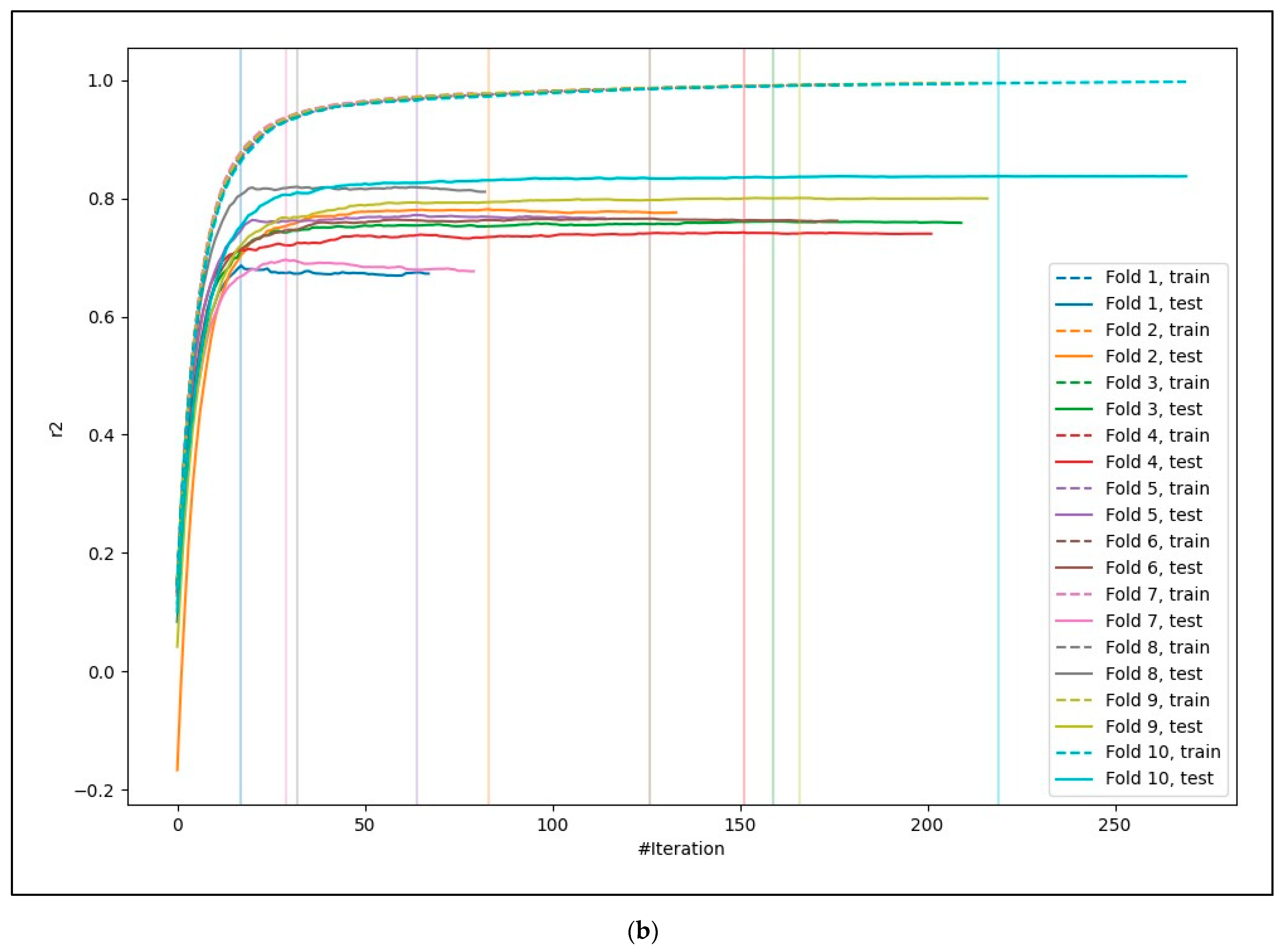
3.1. Model Performance

The evaluation of six models across three datasets is summarized in Table 3. Performance metrics, including Root Mean Squared Error (RMSE) and the coefficient of determination (R2), were averaged over 10 folds to ensure robust comparisons.
These findings highlight the remarkable ability of gradient boosting models, such as XGBoost, LightGBM, and CatBoost, to handle complex, nonlinear, and multi-variable datasets effectively. Among the tested models, XGBoost consistently delivered the best performance across all datasets, achieving the highest accuracy with an RMSE = 0.732, R2 = 0.767 and σr = 0.74, with the definition of σr from [14]. For comparison, traditional GMICE regression models typically report σr values around 1.11 [14], confirming the improved predictive capability of the proposed ML-based approach.
The performance underscores the advantage of gradient boosting frameworks over traditional linear regression models, which serve as the baseline, in capturing intricate patterns and interactions within the data. To align with approaches in the existing literature, we also evaluated the predictive performance of XGBoost when using individual features from dataset 3, as shown in Table 4. The results show that spectral parameters like 0.6 s spectral period and IA achieve the best performance among individual features (RMSE = 0.86 and 0.88, R2 = 0.67 and 0.66, respectively). Specific feature sites are not investigated individually as corrections to physical measurements. In summary, the RMSE and R2 values of the individual features (Table 4) are always worse than those calculated for all three datasets and with each ML model (Table 3), except for the linear regression model.
However, it is important to emphasize that the single-feature analysis is included solely for comparative purposes and does not represent the main objective of the study. In contrast to approaches based on individual predictors, the proposed methodology focuses on capturing nonlinear interactions and dependencies among multiple features—an essential aspect for accurate I_MCS prediction. The results in Table 2 demonstrate that integrating ground motion parameters (GMPs) with site-characteristic corrections (e.g., slope, Vs30) within a gradient boosting framework significantly enhances predictive performance. Such findings underscore the advantage of considering feature interactions over single-variable models, as the combined features account for both the physical properties of ground motion and amplification effects due to site conditions.
Figure 2 shows the learning curves for the XGBoost model during cross-validation. The RMSE trends (Figure 2a) indicate consistent convergence between training and test sets, suggesting good generalization without overfitting. Similarly, the R2 curves (Figure 2b) confirm model robustness, with minimal variability across different data splits.
Figure 3 provides a detailed comparison between predicted and observed I_MCS values. The scatter plot in Figure 3a displays predicted values against ground-truth observations, showing strong predictive performance. Most points cluster along the 45° perfect-agreement line, especially within the mid-range I_MCS interval (4–8). Larger deviations appear at the extremes, with an underestimation of high values and an overestimation of low ones. These patterns reflect challenges in capturing rare or extreme events and point to potential areas for refinement.
Figure 3b illustrates residuals (differences between predicted and observed values) plotted against predicted I_MCS values. The residual distribution is symmetric around the zero line, indicating an absence of major systematic errors. Nonetheless, a slight downward trend suggests a minor bias toward underestimating higher I_MCS values. This observation indicates the need for enhanced feature representation or class-balancing strategies to further improve accuracy across the full intensity spectrum.

3.2. SHAP Analysis: Model Explanation

SHAP analysis provides both global and local perspectives, offering a detailed interpretation of how individual features contribute to I_MCS predictions. This comprehensive approach highlights how the XGBoost model integrates energy parameter, seismic propagation and site-specific corrections, resulting in robust and interpretable predictions.

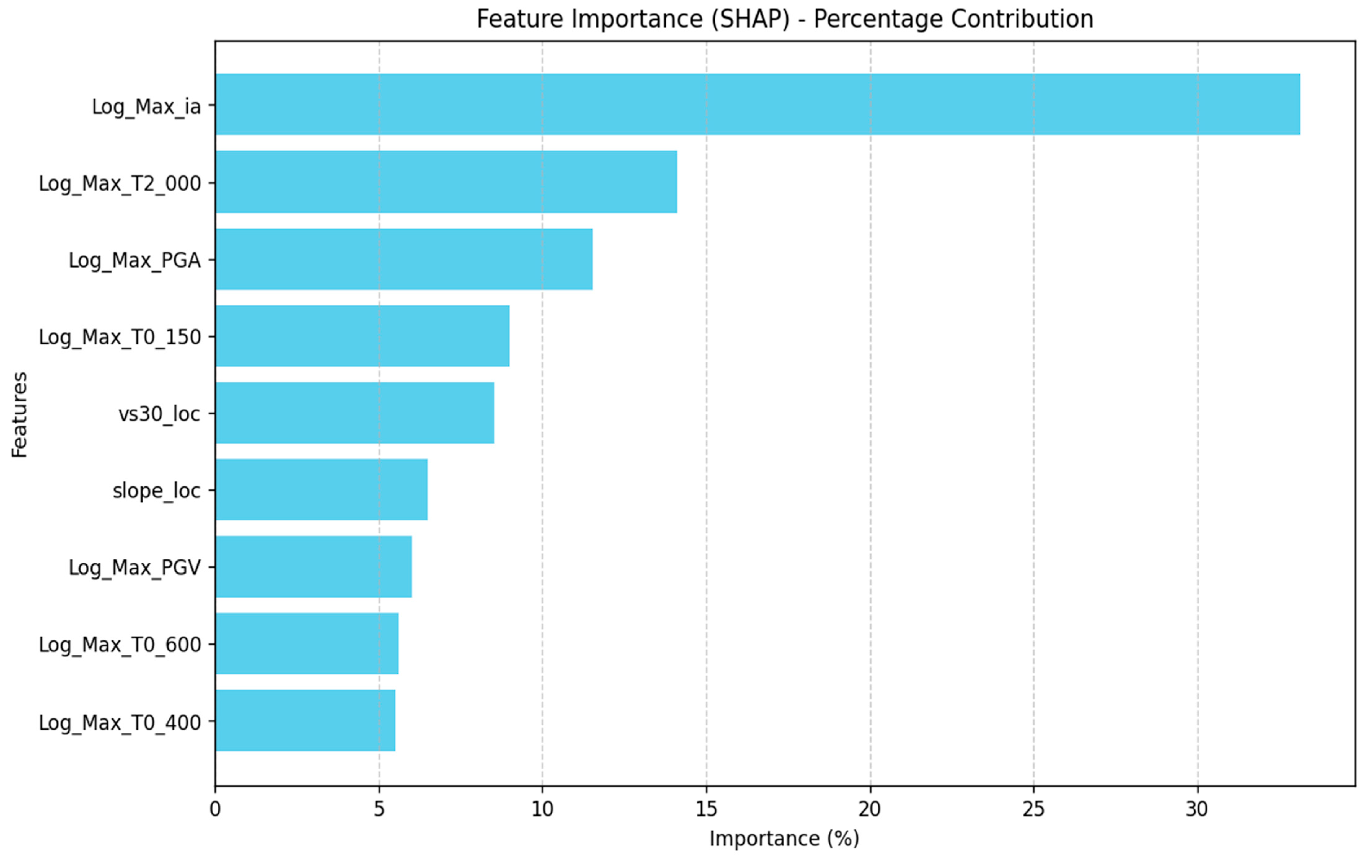
3.2.1. Global Analysis: Feature Ranking Across the Entire Dataset (Figure 4)

The global analysis ranks feature importance based on average SHAP values across the entire dataset (I_MCS 3 to 11). Figure 4 highlights the layered contributions of these features, linking their importance to known seismic phenomena. It should be noted that the ranking of features is closely correlated with the data analysed and their limitations, in particular for extreme intensity predictions (>8.5) due to data imbalances and the over-representation of specific seismic events (e.g., the 2016 sequence in Central Italy).
Figure 4. Global SHAP analysis showing the average absolute SHAP values for each feature across the entire dataset. The ranking highlights the dominant role of regional-scale variables (Log_Max_ia, Log_Max_T2_000, and Log_Max_PGA) in driving predictions, while site-specific features (slope_loc, vs30_loc) also contribute significantly, reflecting their importance in local amplification effects.
Remotesensing 17 01754 g004
The figure also shows that prediction responds to numerous features, of which the three most important ones (IA, 2.0 s spectral period, PGA) cover more than 50% of the contribution and the remaining features each contribute meaningfully to improving prediction, highlighting the complementary role of these variables in refining the model’s accuracy. Furthermore, these results show that it is the relationship between several features that significantly improves prediction. Finally, it can also be notated that immediately below in the ranking of the 2 features that control seismicity at the regional scale (IA, 2.0 s spectral period), we find the 4 features (PGA, 0.15 s spectral period, Vs30 and slope) that characterise the most superficial and therefore site scale part of the seismic damage effects.
As summarised in Table 2, the significance of the features is as follows: (1) IA is the index of earthquake energy, is highly correlated with damage, and is a kind of constant for the entire dataset; (2) 2.00 s spectral period defines a seismic impedance horizon which, according to literature data and calculations with approximate values of S-wave velocities (600–700 m/s), should be between 250 and 400 m. The importance is strongly linked to the seismic events reported in the dataset, which are mostly in Central Italy ([44] for L’Aquila 2009 earthquake; [45] for Central Italy 2016 earthquakes); (3) Vs30 and slope are the accelerometric station-locality correction features that describe the site effects in the strict sense and are placed in the middle of the ranking because, as easy to demonstrate, not at all sites are there lithostratigraphic and/or geomorphological amplifications, and therefore corrections are also more or less important; (4) the interpretation of the other spectral periods (0.4 s and 0.6 s) is more difficult, because they represent horizons of seismic impedance contrasts that are shallower than 0.2 s and therefore have different meanings for different instances (localities) of the dataset. Figure 4 thus shows that considering a statistical average for the entire dataset, one feature is more important than the others, but on its own it fails to robustly evaluate the I_MCS of the localities considered.

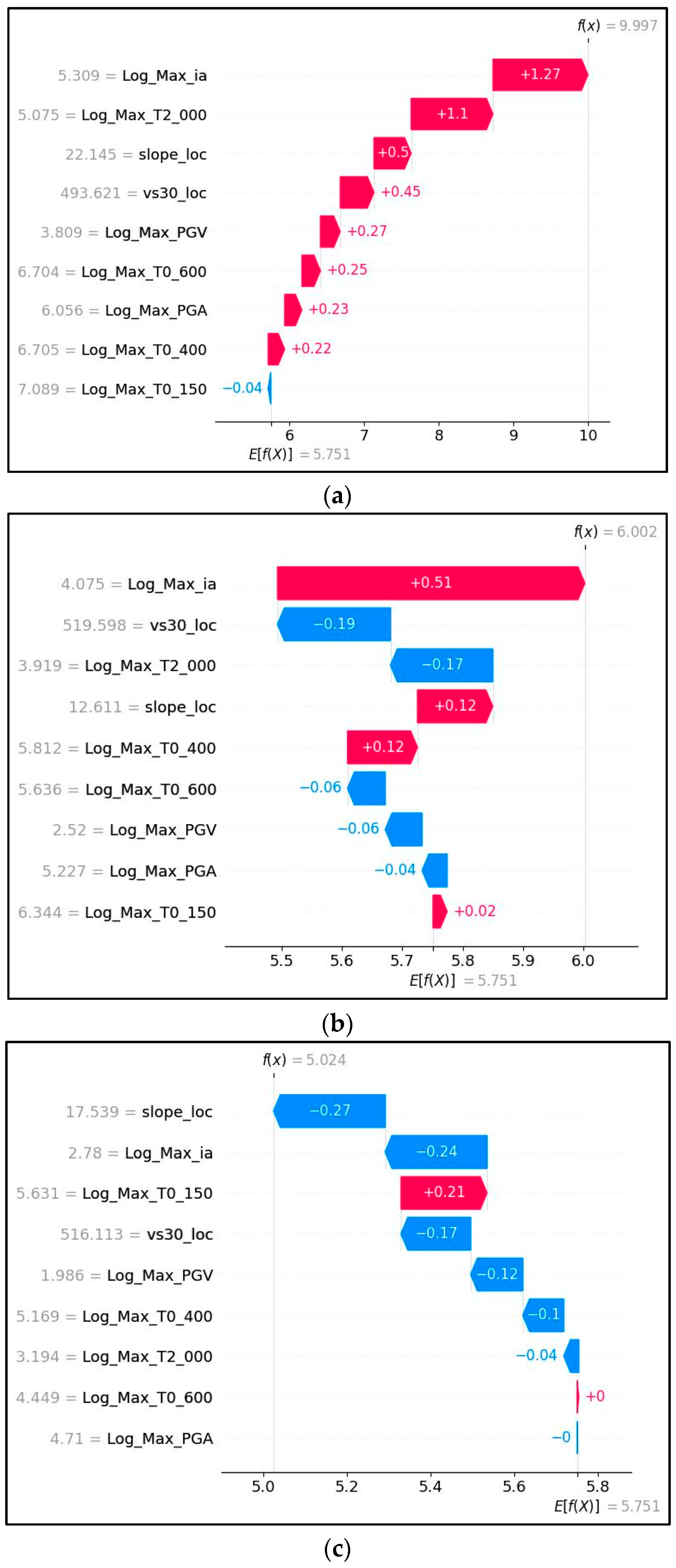
3.2.2. Local Analysis: Insights from the 30 October 2016 Earthquake (Figure 5)

To explore how global importance translates into local importance, we analysed three representative cases from the 30 October 2016 earthquake (Central Italy), focusing on localities at similar epicentral distances (~19 km): Accumoli, Montemonaco, and Poggiodomo. The SHAP waterfall plots (Figure 5) decompose the predicted I_MCS for these localities, showcasing the relative contributions of regional and site features. In the figure, the value of 5.751 is an algorithmic mathematical average of SHAP and the values shown in grey to the left of the features are the actual physical values. Leaving aside the role of AI (is a sort of constant), which is always important in all three localities (and in the entire dataset), in Accumoli (I_MCS = 9.997), the prediction is dominated by regional feature 0.2 s spectral period (+1.1). However, site features such as slope (+0.5) and Vs30 (+0.45) also play a significant role, reflecting the interplay between seismic waves path and site-specific amplification effects correction. We emphasise that, in this case, all features with more or less importance ‘pull’ towards higher than the statistical mean I_MCS (5.75) of the entire dataset. For Montemonaco (I_MCS = 6.002), the importance of the comparison between regional and site features is more balanced. Positive impact from slope (+0.12) is counteracted by negative contributions from Vs30 (−0.19) and 0.2 s spectral period (−0.17), highlighting the complex interaction between propagation effects and site conditions. In Poggiodomo (I_MCS = 5.024) slope (−0.27) is the most important feature contributing negatively. This shift underscores the increasing importance of site-specific corrections in lower-intensity predictions. These examples demonstrate how the model dynamically adjusts feature importance based on the seismic context, effectively balancing the contributions of regional and site factors.
Figure 5. Local SHAP analysis, waterfall plots for three predictions corresponding to localities affected by the 30 October 2016 earthquake: (a) Accumoli (I_MCS = 9.997); (b) Montemonaco (I_MCS = 6.002); (c) Poggiodomo (I_MCS = 5.024). Each plot illustrates the decomposition of the predicted I_MCS value into contributions from regional and local features. The three localities, all approximately 19 km from the epi-centre, demonstrate how the model dynamically integrates feature interactions to reflect site-specific and regional effects.
Remotesensing 17 01754 g005

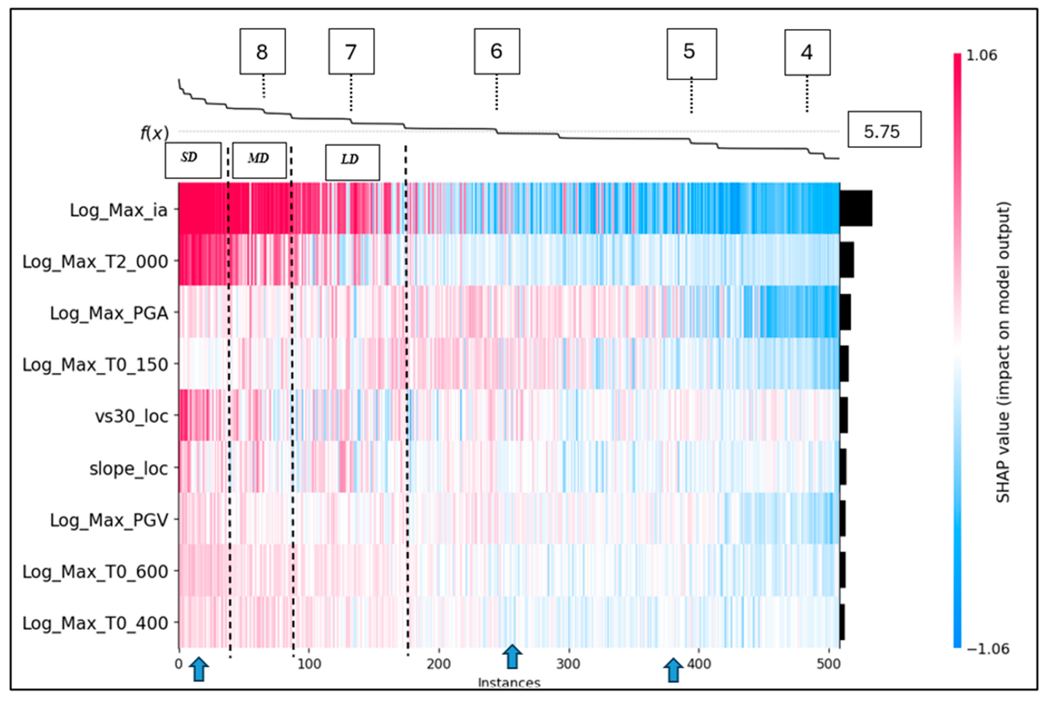
3.2.3. Synthesizing Global and Local Perspectives: The SHAP Heatmap (Figure 6 and Table 5)

After analysing the entire dataset and showing the averages of the feature importances (Figure 4), and after showing the results of the analyses for three localities (Figure 5), we show the relationships between global and local analyses (Figure 6) and the results for I_MCS classes (Table 5). In Table 5, we analysed the results by dividing the I_MCS values into three classes (6.5–7.0, 7.5–8.0, 8.5–11) corresponding to three levels of damage: light, moderate, severe [39]. The SHAP heatmap (Figure 6) provides a comprehensive visualization of feature contributions across the entire dataset. Features are ordered by their global importance (rows), while local importance (columns) are arranged by decreasing I_MCS values as depicted by the black curve f(x) at the top. The predictions for Accumoli, Montemonaco, and Poggiodomo—discussed in Figure 5—correspond to three of the vertical lines shown in Figure 6. Red tones represent positive contributions to I_MCS, increases in I_MCS with respect to the average, while blue tones signify negative contributions, increases in I_MCS with respect to the average prediction. The horizontal line crossing the curve marks the average predicted I_MCS value (5.75), which serves as a reference point for analysing trends. The value of I_MCS = 5.75 is an algorithmic mathematical average that can be interpreted as a binary threshold of transition from no damage to damage but for the identification of the first important threshold related to light damage; we use 6.5 (Grünthal 1998 [26]). The black histograms on the right, consistent with Figure 4, show the global importance of each feature. IA has a positive contribution for almost all localities with I_MCS > 6.5, the same contribution has 0.2 s spectral period but for localities with I_MCS > 7.5. The positive contribution of Vs30 is distributed over all classes but is more evident for higher I_MCS values (>8.5), while the slope contribution is clustered (other considerations are given in the comments to Table 4). This heatmap not only reinforces the importance of globally ranked features but also highlights the adaptability of the model in capturing the nuances of local predictions. Linking global trends to local variability provides an intuitive understanding of how features contribute across different seismic scenarios. Table 5 completes the results of Figure 6. At all damage levels, the regional energy parameter (AI) remains dominant across all I_MCS classes. Similarly, 2.0 s spectral period remains a stable influence, reinforcing the idea that deep impedance contrasts regulate seismic motion consistently, regardless of damage severity. The presence of 2.0 s at all levels highlights the fundamental role of bedrock response in modulating ground motion and justifies the 2.0 s cutoff as a natural boundary between deep crustal propagation and surface response.
Figure 6. SHAP heatmap showing feature contributions across I_MCS predictions. Rows represent features ranked by global importance, and columns correspond to individual locality predictions (instance) ordered by I_MCS. The colour scale indicates the magnitude and direction of the contribution: shades of red signify a positive impact on the prediction, increasing I_MCS values, while shades of blue represent a negative impact, lowering I_MCS values. The black bars on the right indicate the global importance of each feature (Figure 4), as measured by the mean absolute SHAP value. The baseline value of 5.75 I_MCS, represents the average model prediction. From >8.5 data imbalance 2016 Central Italy. Damage levels labels are SD Severe Damage, MD Moderate Damage, LD Light Damage. Key instances of Figure 5 are marked with blue arrows on the instances axis from left to right (Accumoli, Montemonaco, and Poggiodomo).
Remotesensing 17 01754 g006
Table 5. Importance ranking of the most importance feature for different I_MCS classes. Physical station measurements are in standard text, while site-specific corrections are in bold italics. The average distance between the recording station and the locality for each damage group is 1.43 km (σ = 0.94) for light damage, 1.59 km (σ = 0.86) for moderate damage, and 1.59 km (σ = 0.83) for severe damage. These values confirm that the station-to-locality distance remains consistent across different damage levels, supporting the validity of site-specific corrections applied in the analysis.
Importance RankingLight Damage I_MCS 6.5–7.0Moderate Damage
I_MCS 7.5–8.0
Severe Damage
I_MCS 8.5–11
1Log_Max_iaLog_Max_iaLog_Max_ia
2Log_Max_T2_000Log_Max_T2_000Log_Max_T2_000
3Log_Max_T0_600Log_Max_T0_400vs30_loc
4Log_Max_PGALog_Max_T0_600Log_Max_T0_600
5Log_Max_T0_150vs30_locLog_Max_T0_400
6Log_Max_T0_400Log_Max_PGAslope_loc
7slope_locLog_Max_T0_150Log_Max_PGV
8Log_Max_PGVslope_locLog_Max_PGA
9vs30_locLog_Max_PGVLog_Max_T0_150
The role of shallower impedance contrasts, such as those captured at 0.6 s and 0.4 s spectral periods, further supports the interpretation outlined above. The 0.6 s period exhibits stable importance across all I_MCS classes, indicating a broad regional impedance contrast that influences ground motion at an intermediate scale. In contrast, the 0.4 s period displays higher variability, suggesting sensitivity to finer-scale lithostratigraphic heterogeneities. Distinguishing between these two periods is essential for understanding how seismic energy transitions from regional-scale wave propagation to localized site effects.
Table 4 highlights the increasing relevance of site-specific correction factors, namely Vs30 and slope, as damage severity grows. Vs30 emerges during moderate damage scenarios and gains importance in cases of severe damage, reflecting its effectiveness in adjusting shaking intensity based on local soil stiffness. Similarly, slope follows a comparable trend, reinforcing its contribution in correcting for topographic amplification effects. It is important to clarify that these features do not directly represent amplification phenomena, but rather serve as correction proxies that compensate for discrepancies between the shaking recorded at the station and the actual intensity observed at the locality. Their growing importance in high-damage scenarios indicates a critical role in refining intensity estimates under severe shaking conditions.
A further trend observed in Table 5 is the progressive shift in importance from PGA to PGV as damage severity increases. While neither parameter reaches top importance levels, the pattern suggests that PGA dominates the elastic response of structures during light to moderate damage (I_MCS 6.5–7.5), whereas PGV becomes more indicative of collapse in cases of severe structural failure (I_MCS > 8.5). This evolution aligns with the underlying physics: short-period oscillations (T < 0.4 s–0.6 s) are driven primarily by acceleration, whereas intermediate periods (0.6 s–2.0 s) reflect a velocity-dominated structural response. The consistent presence of 0.6 s and 0.4 s periods in this dynamic range reinforces their role in marking the transition between these two regimes.
Finally, the PGA–0.15 s pair exhibits a systematic decrease in relative importance as damage severity increases. While consistently present across all damage levels, these features gradually lose influence in predicting high-intensity outcomes.
We would like to emphasise that the rankings of the three damage classes (Table 5) do not coincide with the overall statistical based ranking obtained with all the data in the dataset (Figure 4) among which the data referring to no damage are also considered.
Figure 7 presents the Partial Dependence Plots (PDP) for the nine main predictors used in the XGBoost model. These plots illustrate the marginal effect of each individual feature on the predicted macroseismic intensity, while holding all other variables constant. As observed, the variation in predicted values across each single feature remains relatively narrow (typically within 1–2 MCS units). This behaviour is expected and highlights a key limitation of PDPs: they only capture average marginal effects and neglect feature interactions. In contrast, the model’s output spans a much broader range (from 3 to over 10 MCS units), which results from non-linear combinations and interactions among multiple features. This is further illustrated in Figure 6 (SHAP heatmap), where high predicted intensities are only achieved when multiple predictors simultaneously contribute positively to the model output. Therefore, while PDPs are useful for capturing general trends, they should not be interpreted in isolation, especially in complex, non-linear models, such as gradient boosting trees. Feature interaction effects are crucial for understanding the full behaviour of the model and should be analyzed with complementary tools like SHAP.
Figure 7. Each subplot shows the marginal effect of a single feature on the predicted macroseismic intensity, while all other features are held constant. The plots reveal the isolated influence of shaking metrics (e.g., Log_Max_PGA, Log_Max_PGV, Log_Max_ia), site-specific parameters (slope_loc, vs30_loc), and spectral accelerations at various periods. Although the individual contribution of each predictor appears limited in magnitude, this reflects the marginal nature of PDPs and highlights the need to consider feature interactions—further explored in the SHAP-based analysis (Figure 6).
Remotesensing 17 01754 g007

4. Discussion

The study demonstrates the effectiveness of integrating advanced machine learning techniques with explainable frameworks to predict macroseismic intensity (I_MCS) from instrumental ground motion parameters (GMPs). By leveraging XGBoost and SHAP analysis, key limitations of traditional Ground Motion to Intensity Conversion Equations are addressed, offering a model that is both accurate and interpretable.
The results highlight significant improvements in predictive performance, with the optimal model achieving RMSE = 0.73 and R2 = 0.76. Inclusion of a diverse set of predictive features—spectral accelerations at key periods (0.15 s, 0.40 s, 0.60 s, 2.0 s), Arias Intensity, PGA, PGV, slope, and Vs30—demonstrates the necessity of capturing nonlinear interactions between multiple seismic parameters and site correction factors.
Based on these findings, the study clarifies the following:
  • inadequacy of individual GMP in accurately predicting I_MCS (Table 3 and Table 4)
  • I_MCS prediction can be significantly improved only by considering multiple features simultaneously (Figure 4 and Figure 5)
  • nonlinear interactions between I_MCS and GMPs (Figure 5 and Figure 6)
  • strong influence of the energy parameter Arias Intensity (Figure 4 and Table 5)
  • low influence of peak parameters (PGA and PGV) (Figure 4 and Table 5).
Arias Intensity consistently emerges as the dominant driver of I_MCS, reinforcing its role as an integrated measure of shaking energy. The ranking of spectral ordinates follows a physically consistent pattern:
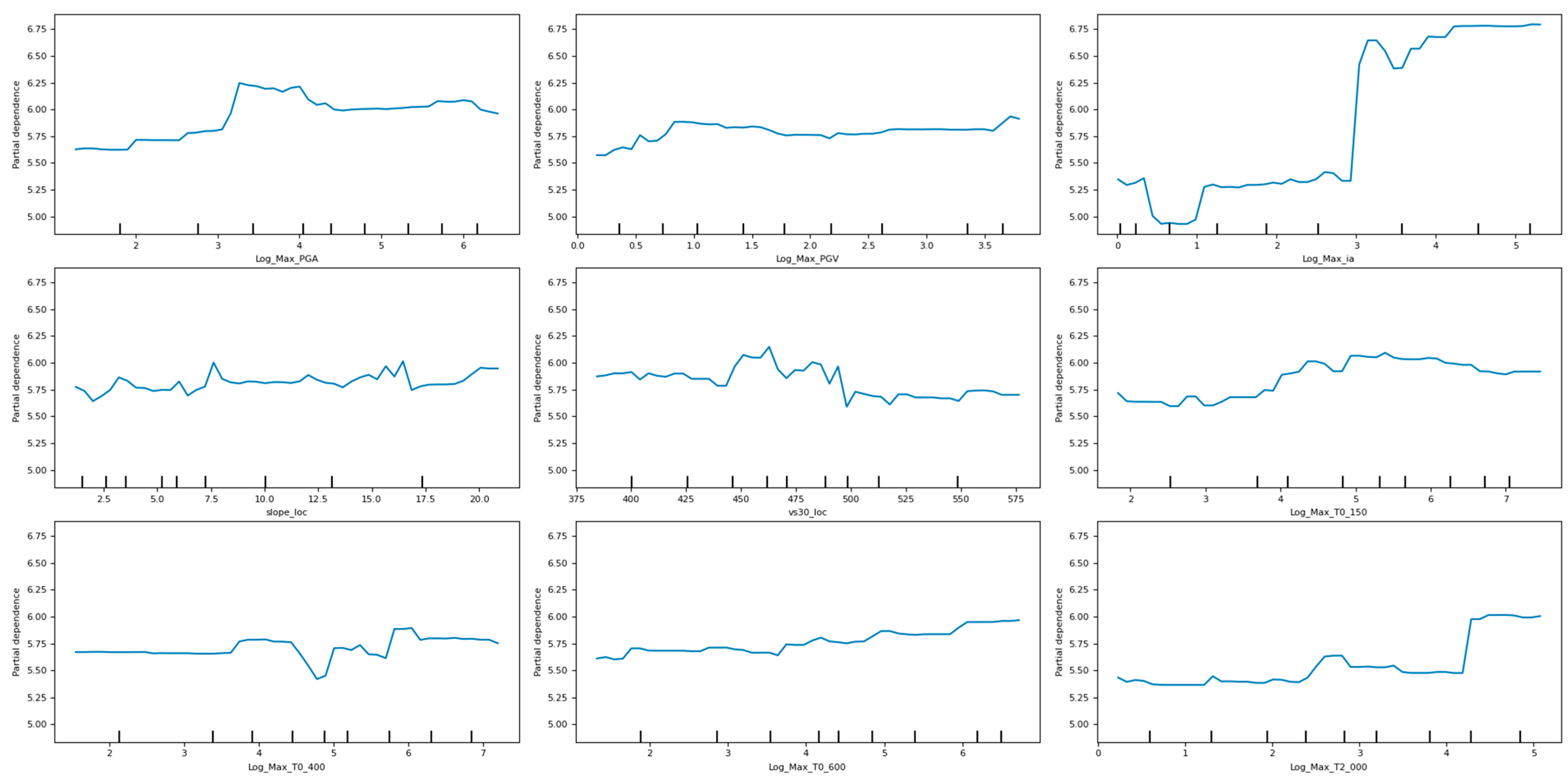
  • 2.0 s spectral period remains a stable driver across all damage levels, reflecting deep-seated impedance contrasts that regulate seismic motion amplification at regional scales.
  • intermediate periods (0.4 s–0.6 s) capture the transition to velocity-based damage mechanics, marking the shift between acceleration-sensitive and deformation-driven effects.
  • Short-period (0.15 s) spectral accelerations and PGA govern light to moderate structural damage, where acceleration-driven forces dominate the response.
A notable observation is the progressive emergence of site-specific corrections (Vs30, slope) in higher damage scenarios (I_MCS > 8.5). These corrections act as adjustments for station-recorded ground motion rather than direct site amplifications, becoming more relevant as shaking intensity increases.
One notable limitation observed during model evaluation is the underestimation of extreme macroseismic intensities (I_MCS > 8.5). The effect is primarily linked to dataset imbalance, as only 7% of observations fall within the highest damage category. To explore potential solutions, an initial experiment was conducted using a classification-based approach with SMOTE for oversampling. However, the combination of the ordinal nature of I_MCS and the limited availability of high-damage cases led to unstable and non-generalizable results. For these reasons, a regression framework was retained, preserving the original data distribution.
To handle uncertainty in high-intensity predictions without introducing synthetic data, a probabilistic extension of the model is currently under development using NGBoost. This method generates not only a central estimate but also a full predictive distribution for each site, enabling the assessment of confidence levels associated with individual predictions. Access to such information is crucial for emergency management, particularly during early response phases when underestimation of damage may delay or compromise intervention strategies. For example, low predicted intensity values in heavily affected areas could hinder timely deployment of rescue teams, distribution of emergency medical supplies, and readiness of nearby healthcare facilities.
The model has been developed with real-time application as a central goal. In collaboration with the Italian Civil Protection Department, the broader system activates automatically following earthquakes of magnitude M ≥ 5.0 and is designed to deliver shakemaps and damage scenarios within 30 min. Outputs include predicted shaking intensity, expected building damage, and estimates of co-seismic landslides or liquefaction that could impact strategic transport routes essential for emergency response.

5. Conclusions

The proposed XGBoost model achieved a 33% reduction in residual standard deviation compared to traditional GMICE methods, demonstrating its enhanced predictive accuracy for macroseismic intensity estimation.
While the model offers substantial advancements in intensity prediction, certain limitations remain, particularly at extreme intensity levels (I_MCS > 8.5). The dataset exhibits a class imbalance, with only 7% of observations falling into the highest damage category, potentially affecting predictive accuracy in these scenarios.
Future work should aim to overcome the limitation by:
  • Expanding the macroseismic dataset to enhance the model’s ability to generalize across a wider range of seismic contexts.
  • Incorporating building vulnerability metrics, such as construction type, age, and material, to better account for structural differences in damage response.
  • Integrating physical seismological metrics, including magnitude, fault distance, and other relevant factors, to improve the accuracy and robustness of damage prediction.
The study highlights the transformative potential of combining advanced data-driven methods with physical seismic principles, providing a robust tool for disaster risk mitigation and seismic hazard management. By bridging the gap between predictive accuracy and interpretability, the framework paves the way for improving seismic resilience in vulnerable regions worldwide.
In the context of emergency management, I_MCS data provide crucial information for evaluating the impact of an earthquake on a regional scale. The efficiency of emergency response systems—comprising both structural elements (buildings, infrastructure, and designated emergency areas) and non-structural components (logistics, emergency personnel, and information management)—depends on an accurate estimation of damage scenarios. These estimates guide the optimal allocation of resources, ensuring a timely and effective civil protection response.
A key contribution of this study is the integration of machine learning techniques with I_MCS data and site-specific correction factors, enhancing macroseismic intensity estimation and damage assessment. However, challenges remain, particularly in accounting for secondary earthquake-induced hazards, such as landslides and liquefaction, which can exacerbate structural damage and disrupt critical infrastructure. The ability to evaluate these cascading effects is essential for understanding the functional resilience of emergency response networks, including transportation routes, medical facilities, and communication systems.
The role of seismic hazard and local site effects in determining the operability of emergency response systems has been previously explored by Mori et al. [46], who highlighted the importance of integrating seismic impact assessments with infrastructure vulnerability analysis. Building on the current methodology, a modernized framework should incorporate the following:
  • Macroseismic intensity prediction model for assessing direct earthquake damage to buildings and infrastructure.
  • Landslide and liquefaction predictive models, calibrated with ground motion parameters and geospatial predictors.
  • Network-based impact assessments, considering disruptions to transportation and emergency response logistics.
Future research should explore the integration of I_MCS with remote sensing-based impact assessments, such as Copernicus Emergency Management Service (EMS) maps and NASA ARIA Damage Proxy Maps, to enhance real-time situational awareness. The fusion of satellite-derived proxies (e.g., InSAR ground deformation, land cover changes, AI-driven damage detection) with ground-based macroseismic intensity records could improve multi-hazard modelling and network resilience analysis.
Ultimately, a systemic approach linking shaking intensity, structural damage, landslides, liquefaction, and network disruptions could provide a more comprehensive framework for assessing emergency response effectiveness. By integrating AI-driven analysis, geospatial big data, and remote sensing observations, future advancements can support real-time decision-making, ensuring faster and more effective disaster response in earthquake-affected regions.
Finally, we note that recent developments in seismic data processing within the oil and gas sector have showcased the versatility of machine learning in handling complex geophysical datasets [47] and reference within]. While these applications differ from the emergency response focus of this study, they highlight the potential for cross-domain methodological innovation and could inspire future advancements in intensity prediction and multi-hazard assessment frameworks.

Author Contributions

F.M. was responsible for developing the machine learning framework and conducting the associated analyses. G.N. and F.M. jointly contributed to the writing of the manuscript, with F.M. focusing on the initial drafts and G.N. refining and finalizing the text. Both authors reviewed and approved the final manuscript, contributing equally to the overall conceptualization and interpretation of the study. All authors have read and agreed to the published version of the manuscript.

Funding

This work was funded by the Italian Department of Civil Protection, Presidency of the Council of Ministers “Accordo URBISIT 9 tra Presidenza del Consiglio dei Ministri Dipartimento della Protezione Civile e CNR IGAG”.

Data Availability Statement

Data used in this study are sourced from the INGe dataset (Oliveti et al., 2021 [28]), ITACA (Felicetta et al., 2023 [29]), Vs dataset (Mori et al., 2024 [32]).

Acknowledgments

The authors would like to thank P. Galli of the Italian Civil Protection Department (Seismic Risk Office) for productive discussions.

Conflicts of Interest

The authors declare no conflicts of interest.

Abbreviations

The following abbreviations are used in this manuscript:
I_MCSMacroseismic Intensity
EMS-98European Macroseismic Scale 1998
GMPGround Motion Parameter
PGAPeak Ground Acceleration
PGVPeak Ground Velocity
IAArias Intensity
Vs30Time-averaged shear wave velocity over the top 30 m of soil
GMICEGround Motion to Intensity Conversion Equations
DBMI15Database Macrosismico Italiano 2015
CPTI15Catalogo Parametrico dei Terremoti Italiani 2015
ITACAItalian Accelerometric Archive
SHAPShapley Additive Explanations
XGBoosteXtreme Gradient Boosting
LightGBMLight Gradient Boosting Machine
CatBoostCategorical Boosting
MLMachine Learning
RMSERoot Mean Square Error
R2Coefficient of Determination
AutoMLAutomated Machine Learning
INGeIntensity-ground Motion Dataset for Italy
MLJARMachine Learning Jar (AutoML Platform)
σrStandard Deviation
T0_150, T0_400, T0_600, T2_000Spectral acceleration periods (0.15 s, 0.4 s, 0.6 s, 2 s)
DEMDigital Elevation Model
MERITMulti-Error-Removed Improved-Terrain DEM

References

  1. Cito, P.; Chioccarelli, E.; Iervolino, I. Macroseismic intensity hazard maps for Italy based on a recent grid source model. Bull. Earthq. Eng. 2022, 20, 2245–2258. [Google Scholar] [CrossRef]
  2. Galli, P.; Bosi, V.; Piscitelli, S.; Giocoli, A.; Scionti, V. Late Holocene earthquakes in southern Apennine: Paleoseismology of the Caggiano fault. Int. J. Earth Sci. 2006, 95, 855–870. [Google Scholar] [CrossRef]
  3. Galli, P.; Molin, D. Il Terremoto del 1905 Della Calabria Meridionale. Studio Analitico Degli Effetti ed Ipotesi Sismogenetiche; IlMioLibro: Perugia, Italy, 2007; 124p, Available online: https://emidius.mi.ingv.it/ASMI/study/GALMO007 (accessed on 18 February 2025).
  4. Faenza, L.; Michelini, A. Regression analysis of MCS intensity and ground motion parameters in Italy and its application in ShakeMap. Geophys. J. Int. 2010, 180, 1138–1152. [Google Scholar] [CrossRef]
  5. Rotondi, R.; Varini, E.; Brambilla, C. Probabilistic modelling of macroseismic attenuation and forecast of damage scenarios. Bull. Earthq. Eng. 2016, 14, 1777–1796. [Google Scholar] [CrossRef]
  6. Rossi, A.; Tertulliani, A.; Azzaro, R.; Graziani, L.; Rovida, A.; Maramai, A.; Pessina, V.; Hailemikael, S.; Buffarini, G.; Bernardini, F.; et al. The 2016–2017 earthquake sequence in Central Italy: Macroseismic survey and damage scenario through the EMS-98 intensity assessment. Bull. Earthq. Eng. 2019, 17, 2407–2431. [Google Scholar] [CrossRef]
  7. Del Mese, S.; Graziani, L.; Meroni, F.; Pessina, V.; Tertulliani, A. Considerations on using MCS and EMS-98 macroseismic scales for the intensity assessment of contemporary Italian earthquakes. Bull. Earthq. Eng. 2023, 21, 4167–4189. [Google Scholar] [CrossRef]
  8. Locati, M.; Camassi, R.; Rovida, A.; Ercolani, E.; Bernardini, F.; Castelli, V.; Caracciolo, C.H.; Tertulliani, A.; Rossi, A.; Azzaro, R.; et al. Database Macrosismico Italiano (DBMI15); Versione 4.0; Istituto Nazionale di Geofisica e Vulcanologia (INGV): Rome, Italy, 2022. [Google Scholar] [CrossRef]
  9. Rovida, A.; Locati, M.; Camassi, R.; Lolli, B.; Gasperini, P.; Antonucci, A. Italian Parametric Earthquake Catalogue (CPTI15); Vers. 4.0; Istituto Nazionale di Geofisica e Vulcanologia (INGV): Rome, Italy, 2022. [Google Scholar] [CrossRef]
  10. Wald, D.J.; Quitoriano, V.; Heaton, T.H.; Kanamori, H. Relationships between peak ground acceleration, peak ground velocity, and modified Mercalli intensity in California. Earthq. Spectra 1999, 15, 557–564. [Google Scholar] [CrossRef]
  11. Masi, A.; Chiauzzi, L.; Nicodemo, G.; Manfredi, V. Correlations between macroseismic intensity estimations and ground motion measures of seismic events. Bull. Earthq. Eng. 2020, 18, 1899–1932. [Google Scholar] [CrossRef]
  12. Vannucci, G.; Lolli, B.; Gasperini, P. A theoretical comparison among macroseismic scales used in Italy. Bull. Earthq. Eng. 2024, 22, 4245–4263. [Google Scholar] [CrossRef]
  13. Cataldi, L.; Tiberi, L.; Costa, G. Estimation of MCS intensity for Italy from high quality accelerometric data, using GMICEs and Gaussian Naïve Bayes Classifiers. Bull. Earthq. Eng. 2021, 19, 2325–2342. [Google Scholar] [CrossRef]
  14. Oliveti, I.; Faenza, L.; Michelini, A. New reversible relationships between ground motion parameters and macroseismic intensity for Italy and their application in ShakeMap. Geophys. J. Int. 2022, 231, 1117–1137. [Google Scholar] [CrossRef]
  15. Arias, A. A measure of earthquake intensity. In Seismic Design for Nuclear Power Plants; Hansen, R.J., Ed.; MIT Press: Cambridge, MA, USA, 1970. [Google Scholar]
  16. Trifunac, M.D.; Brady, A.G. A study on the duration of strong earthquake ground motion. Bull. Seismol. Soc. Am. 1975, 65, 581–626. [Google Scholar]
  17. Kramer, S.L. Geotechnical Earthquake Engineering; Prentice Hall: Upper Saddle River, NJ, USA, 1996. [Google Scholar]
  18. Bertero, V.V.; Mahin, S.A.; Herrera, R.A. Aseismic design implications of strong-motion records. Earthq. Eng. Struct. Dyn. 1978, 6, 31–42. [Google Scholar] [CrossRef]
  19. Papageorgiou, A.S.; Aki, K. A specific barrier model for the quantitative description of inhomogeneous faulting and the prediction of strong ground motion. Bull. Seismol. Soc. Am. 1983, 73, 693–722. [Google Scholar] [CrossRef]
  20. Bard, P.Y.; Bouchon, M. The two-dimensional resonance of sediment-filled valleys. Bull. Seismol. Soc. Am. 1985, 75, 519–541. [Google Scholar] [CrossRef]
  21. Boore, D.M.; Joyner, W.B. Site amplifications for generic rock sites. Bull. Seismol. Soc. Am. 1997, 87, 327–341. [Google Scholar] [CrossRef]
  22. Spudich, P.; Hellweg, M.; Lee, W.H.K. Directional topographic site response at Tarzana observed in aftershocks of the 1994 Northridge, California, earthquake: Implications for mainshock motions. Bull. Seismol. Soc. Am. 1996, 86, S193–S208. [Google Scholar] [CrossRef]
  23. Ashford, S.A.; Sitar, N. Analysis of topographic amplification of inclined shear waves in a steep coastal bluff. Bull. Seismol. Soc. Am. 1997, 87, 692–700. [Google Scholar] [CrossRef]
  24. Borcherdt, R.D. Estimates of site-dependent response spectra for design (methodology and justification). Earthq. Spectra. 1994, 10, 617–653. [Google Scholar] [CrossRef]
  25. Boore, D.M.; Thompson, E.M.; Cadet, H. Regional correlations of VS30 and velocities averaged over depths less than and greater than 30 m. Bull. Seismol. Soc. Am. 2011, 101, 3046–3059. [Google Scholar] [CrossRef]
  26. Grünthal, G. (Ed.) European Macroseismic Scale 1998 (EMS-98); Cahiers du Centre Européen de Géodynamique et de Séismologie: Luxembourg, 1998; Volume 15. [Google Scholar]
  27. Worden, C.B.; Gerstenberger, M.C.; Rhoades, D.A.; Wald, D.J. Probabilistic relationships between ground-motion parameters and modified Mercalli intensity in California. Bull. Seismol. Soc. Am. 2012, 102, 204–221. [Google Scholar] [CrossRef]
  28. Oliveti, I.; Faenza, L.; Michelini, A. INGe: Intensity-Ground Motion Dataset for Italy [Dataset] Version 2. Zenodo. 2021. Available online: https://zenodo.org/records/4623732 (accessed on 13 May 2025).
  29. Felicetta, C.; Russo, E.; D’Amico, M.; Sgobba, S.; Lanzano, G.; Mascandola, C.; Pacor, F.; Luzi, L. ITACA: The Italian Accelerometric Archive. 2023. Available online: https://itaca.mi.ingv.it (accessed on 13 May 2025).
  30. Yamazaki, D. MERIT DEM: A global DEM derived from multiple datasets. Water Resour. Res. 2017, 53, 5549–5573, Dataset Availability 1987-01-01T00:00:00Z–2017-01-01T00:00:00Z. [Google Scholar]
  31. Mori, F.; Mendicelli, A.; Moscatelli, M.; Romagnoli, G.; Peronace, E.; Naso, G. A new Vs30 map for Italy based on the seismic microzonation dataset. Eng. Geol. 2020, 275, 105745. [Google Scholar] [CrossRef]
  32. Mori, F.; Mendicelli, A.; Moscatelli, M.; Varone, C. Shear Wave Velocity Profiles Dataset. Zenodo. 2024. Available online: https://zenodo.org/records/11263471 (accessed on 13 May 2025).
  33. Gomez-Capera, A.A.; D’Amico, M.; Lanzano, G.; Locati, M.; Santulin, M. Relationships between ground motion parameters and macroseismic intensity for Italy. Bull. Earthq. Eng. 2020, 18, 5143–5164. [Google Scholar] [CrossRef]
  34. Cornou, C.; Bard, P.-Y.; Dietrich, M. Contribution of dense array analysis to the identification and quantification of basin-edge-induced waves. Part I: Methodology. Bull. Seismol. Soc. Am. 2003, 93, 2604–2623. [Google Scholar] [CrossRef]
  35. Bard, P.Y.; Brian, E.; Tucker, E. Underground and ridge site effects: A comparison of observation and theory. Bull. Seismol. Soc. Am. 1985, 75, 905–922. [Google Scholar] [CrossRef]
  36. Lundberg, S.M.; Lee, S.-I. A unified approach to interpreting model predictions. Adv. Neural Inf. Process. Syst. 2017, 30, 4765–4774. [Google Scholar] [CrossRef]
  37. Draper, N.R.; Smith, H. Applied Regression Analysis, 3rd ed.; Wiley: Hoboken, NJ, USA, 1998. [Google Scholar] [CrossRef]
  38. Breiman, L. Random Forests. Mach. Learn. 2001, 45, 5–32. [Google Scholar] [CrossRef]
  39. Chen, T.; Guestrin, C. XGBoost: A scalable tree boosting system. In Proceedings of the 22nd ACM SIGKDD International Conference on Knowledge Discovery and Data Mining, San Francisco, CA, USA, 13–17 August 2016; pp. 785–794. [Google Scholar] [CrossRef]
  40. Ke, G.; Meng, Q.; Finley, T.; Wang, T.; Chen, W.; Ma, W.; Ye, Q.; Liu, T.Y. LightGBM: A highly efficient gradient boosting decision tree. In Proceedings of the 31st International Conference on Neural Information Processing Systems, Long Beach, CA, USA, 4–9 December 2017; pp. 3149–3157. [Google Scholar]
  41. Prokhorenkova, L.; Gusev, G.; Vorobev, A.; Dorogush, A.V.; Gulin, A. CatBoost: Unbiased boosting with categorical features. Adv. Neural Inf. Process. Syst. 2018, 31, 6638–6648. [Google Scholar]
  42. LeCun, Y.; Bengio, Y.; Hinton, G. Deep learning. Nature 2015, 521, 436–444. [Google Scholar] [CrossRef]
  43. Shapley, L. A theoretical framework for n-person cooperative games. In Contributions to the Theory of Games II; Kuhn, H., Tucker, A., Eds.; Princeton University Press: Princeton, NJ, USA, 1953; pp. 307–317. [Google Scholar] [CrossRef]
  44. Bruno, P.P.G.; Villani, F.; Improta, L. High-resolution seismic imaging of fault-controlled basins: A case study from the 2009 Mw 6.1 central Italy earthquake. Tectonics 2022, 41, e2022TC007207. [Google Scholar] [CrossRef]
  45. Buttinelli, M.; Petracchini, L.; Maesano, F.E.; D’Ambrogi, S.; Scrocca, D.; Marino, M.; Capotorti, F.; Bigi, S.; Cavinato, G.P.; Mariucci, M.T.; et al. The impact of structural complexity, fault segmentation, and reactivation on seismotectonics: Constraints from the upper crust of the 2016–2017 Central Italy seismic sequence area. Tectonophysics 2021, 810, 228861. [Google Scholar] [CrossRef]
  46. Mori, F.; Gena, A.; Mendicelli, A.; Naso, G.; Spina, D. Seismic emergency system evaluation: The role of seismic hazard and local effects. Eng. Geol. 2020, 270, 105587. [Google Scholar] [CrossRef]
  47. Lawal, A.; Yang, Y.; He, H.; Baisa, N.L. Machine Learning in Oil and Gas Exploration: A Review. IEEE Access 2024, 12, 19035–19058. [Google Scholar] [CrossRef]
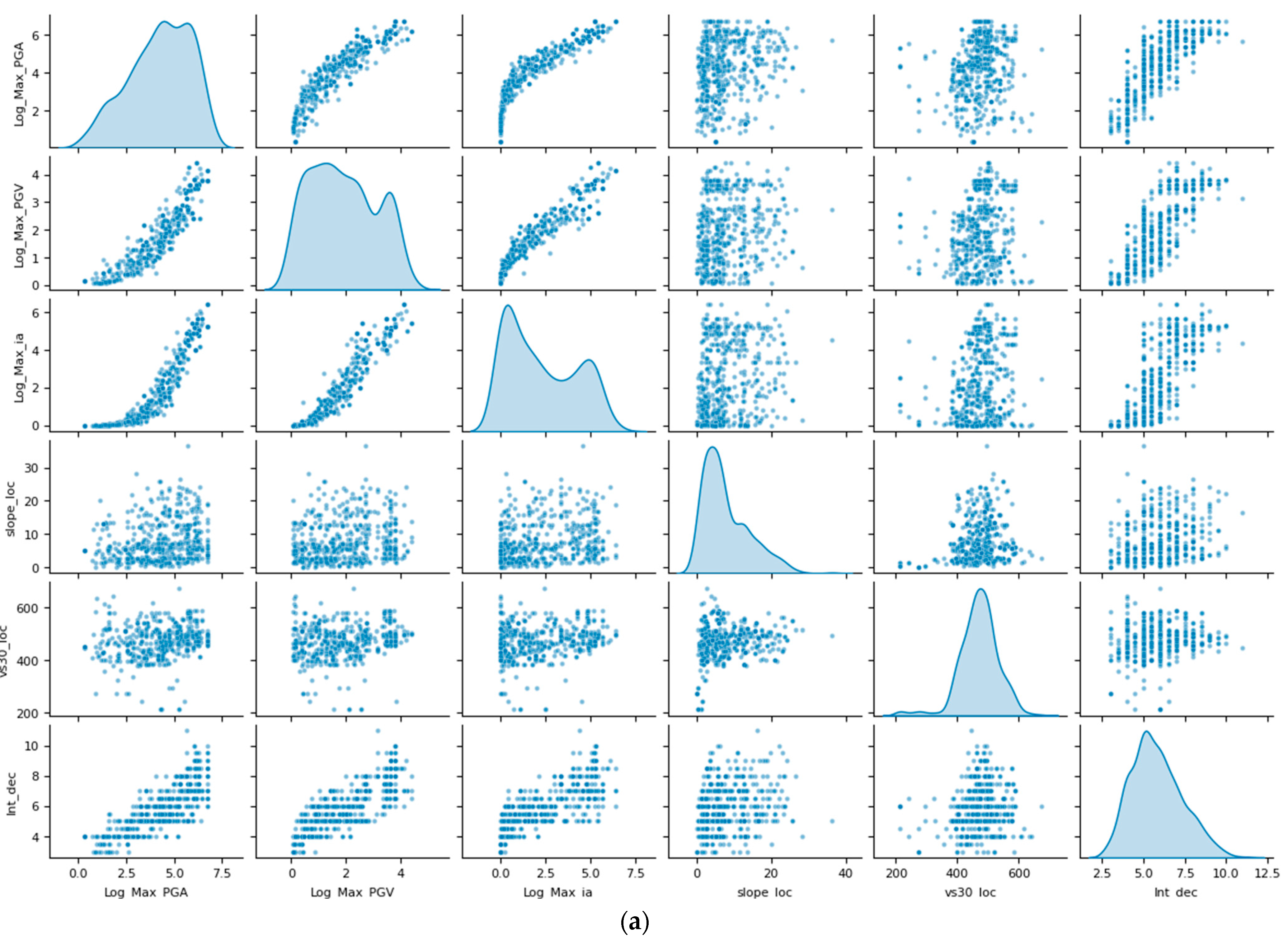
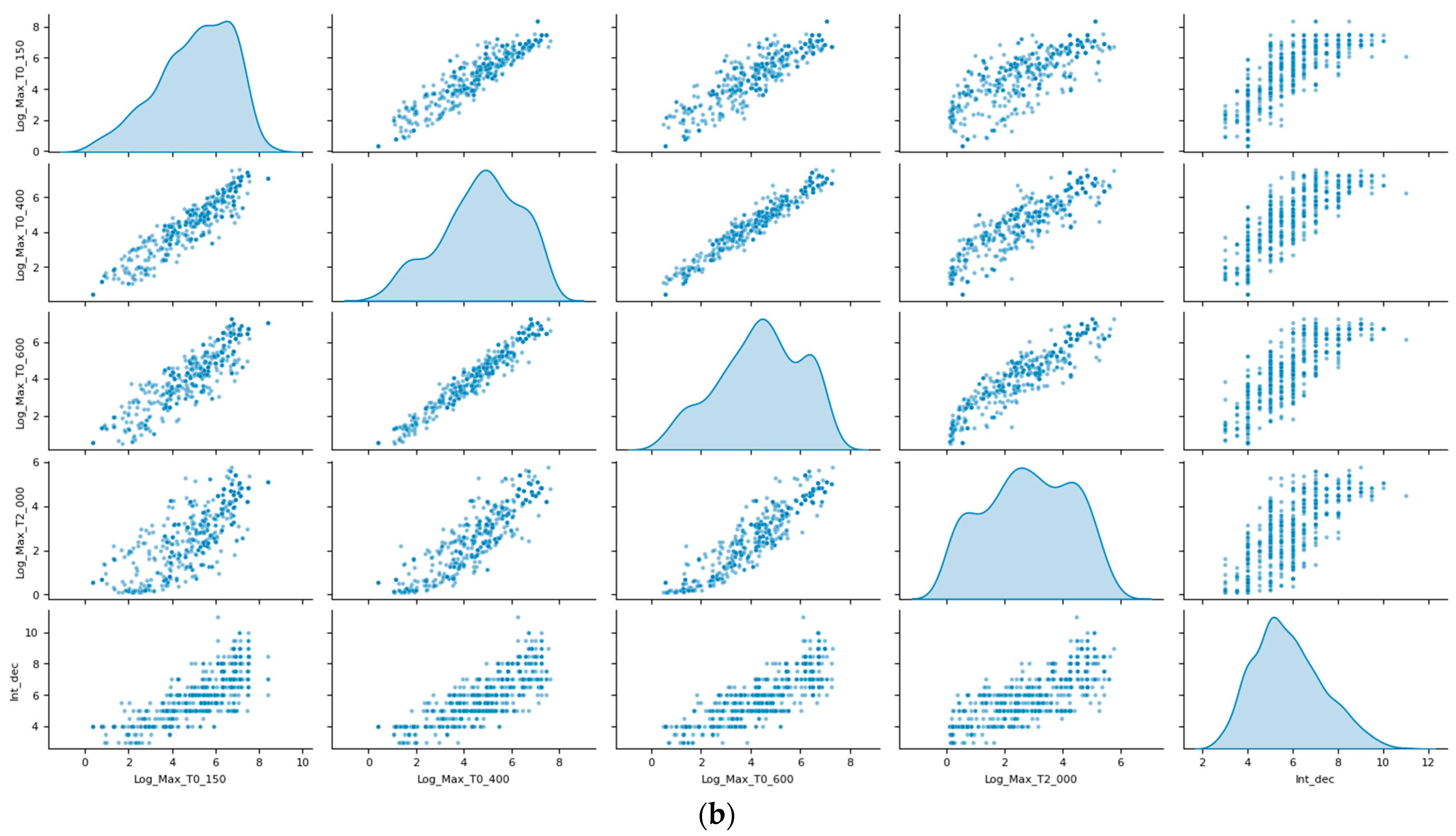
Figure 1. Relationships among the dataset 3 for input and output features: (a) Relationships among Log_Max_PGA, Log_Max_PGV, Log_Max_ia, slope_loc, and vs30_loc. The diagonal elements display histograms for individual distributions, while off-diagonal scatterplots highlight pairwise relationships, revealing strong correlations among peak ground motion features and their interaction with site-specific variables; (b) Relationships among Log_Max_T0_150, Log_Max_T0_400, Log_Max_T0_600, Log_Max_T2_000.
Remotesensing 17 01754 g001aRemotesensing 17 01754 g001b
Figure 2. Learning curves for the XGBoost model during 10-fold cross-validation: (a) Root Mean Square Error (RMSE) as a function of number of iterations; (b) R2 score. Both metrics are shown for the training (dashed lines) and test (solid lines) sets across all folds. The consistent convergence between training and test curves indicates effective generalization without overfitting. Minor variations among folds reflect the impact of data splits on model performance.
Remotesensing 17 01754 g002aRemotesensing 17 01754 g002b
Figure 3. Model evaluation plots: (a) Scatter plot comparing predicted (y_pred) vs. observed values (y), with the red dashed line indicating perfect agreement and the blue line showing the regression trend; (b) Residuals vs. predicted values, with the red dashed line representing the zero-residual line and the green line showing the residual trend.
Remotesensing 17 01754 g003
Table 1. Seismic parameters categorized by measurement type: physical recordings at stations, site-specific corrections, and macroseismic intensity as the output. The table highlights each parameter’s role in damage severity, from regional wave propagation to site amplification effects.
Datasets Feature Label (Type)Description
(in Bold as Cited in the Text)
Role on Earthquake
Damage Potential
Max_ia (Physical)Maximum among the two horizontal components of the Arias Intensity (IA) measured at the stationGoverns damage intensity at all scales; represents the total energy released by seismic shaking [15,16]
Max_PGA (Physical)Maximum among the two horizontal components of the Peak Ground Acceleration (PGA) measured at the stationMore relevant for light damage; peak accelerations dominate the elastic response of structures and are associated with short-period spectral components [17]
Max_PGV (Physical)Maximum among the two horizontal components of the Peak Ground Velocity (PGV) measured at the stationMore important for severe damage and collapses; accumulated deformation plays important role, especially in longer-duration shaking [18,19]
Max_Tx_xx (Physical)Maximum among the two horizontal components of the spectral acceleration at specific periods (e.g., 0.15 s, 0.40 s, 0.60 s, 2.00 s spectral periods) measured at the stationIndicator of impedance contrasts at different depths, corresponding to various seismic horizons that regulate wave propagation [20,21]
slope_loc (accelerometric station-locality correction)Slope correction at the locality, sampled from the MERIT Digital Elevation Model at 3 arcsecond resolution (~90 m at the equator)Correction factor accounting for topographic effects in local intensity estimations. Topographic amplification is more pronounced on steep slopes and rigid substrates [22,23]
vs30_loc (accelerometric station-locality correction)Vs30 correction at the locality, representing the time-averaged shear wave velocity over the top 30 m of soil (m/s), predicted with kriging from Vs dataset (https://zenodo.org/records/11263471, accessed on 18 February 2025)Correction factor adjusting the ground motion recorded at the station to reflect site-specific shear wave velocity conditions. Soil stiffness modulates the local seismic response and influences ground motion amplification [24,25]
int_dec (OUTPUT)Decimal value of macroseismic intensity (I_MCS) at the locality, based on the DBMI15 manualMacroseismic intensity (I_MCS) estimated at the locality, integrating ground shaking, site effects, and structural vulnerability [26,27]
Table 2. Hyperparameter optimization using OPTUNA.
ParameterOptuna RangeBest Value
learning_rate0.02–0.50.05
max_depth3–105
min_child_weight0.5–61
subsample0.6–1.00.8
colsample_bytree0.6–1.00.8
gamma0–20
lambda0.1–5.01
Table 3. Performance metrics of the ML models evaluated using the AutoML MLJAR framework. Models were ranked based on their RMSE and R2, with XGBoost achieving the best performance (in bold) among the tested models.
Dataset: FeaturesModelRMSER2
Dataset 1: Max_PGA, Max_PGV, Max_T0_300, Max_T1_000, Max T3_000Linear regression0.9650.581
LightGBM0.8300.680
Xgboost0.8100.710
CatBoost0.8230.685
Neural Network0.9560.588
Random Forest0.8880.640
Dataset 2: Max_ia, Max_PGA, Max_PGV, Max_T0_300, Max T1_000, Max T3_000
slope_loc, vs30_loc
Linear regression0.9000.648
LightGBM0.7920.714
Xgboost0.7700.740
CatBoost0.7930.713
Neural Network0.8770.666
Random Forest0.7940.726
Dataset 3: Max_ia, Max_PGA, Max_PGV, Max_T0_150, Max_T0_400, Max_T0_600 Max_T2_000, slope_loc, vs30_locLinear regression0.8950.652
LightGBM0.7430.760
Xgboost0.7320.767
CatBoost0.7470.758
Neural Network0.9050.644
Random Forest0.8120.729
Table 4. Performance of single features in predicting I_MCS using XGBoost. The table highlights the variability in predictive power across individual features.
FeatureRMSE (XGBoost)R2
(XGBoost)
Max_T0_6000.860.67
Max_ia0.880.66
Max_T0_1500.890.64
Max_PGV0.90.64
Max_PGA0.910.63
Max_T0_4000.910.63
Max_T2_0000.920.62
Disclaimer/Publisher’s Note: The statements, opinions and data contained in all publications are solely those of the individual author(s) and contributor(s) and not of MDPI and/or the editor(s). MDPI and/or the editor(s) disclaim responsibility for any injury to people or property resulting from any ideas, methods, instructions or products referred to in the content.

