Figure 1.
Orthomosaic representation of the experimental field captured by a multi-spectral camera. The image shows the field comprising five blocks with four rows in each of the blocks. The five blocks are labeled as 100s to 500s, where they are addressed as 101, 102, 103, and 104 for the four rows in block #100. Each row is subdivided into four plots (A, B, C, D) of 20 plants each, with each plot being identified by its row number and column letter. In each of the rows, one plot is susceptible to PVY, while the other three plots are resistant. The resistant cultivars are comparatively skinnier than the susceptible cultivars. For example, plot 101B is the experimental plot and is susceptible to PVY. Some ground control points with checkerboard patterns are placed along the west side of the field, which helps in manually identifying the individual images captured by the camera.
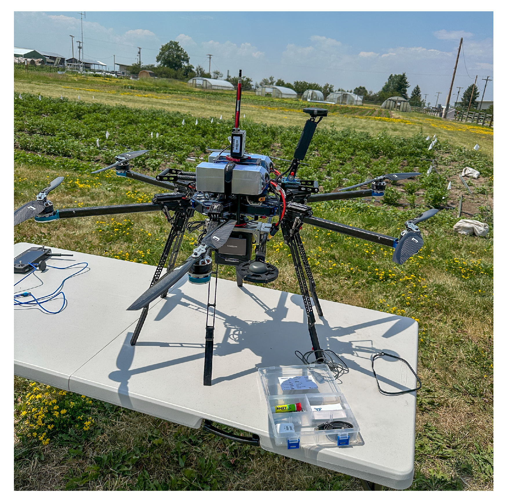
Figure 2.
Resonon Pika L hyperspectral camera is mounted on the Vision Aerial Vector Hexacopter drone. A dual GPS/IMU and a downwelling irradiance sensor were added for better GPS accuracy and to correct the reflection of lights in the captured images.
Figure 2.
Resonon Pika L hyperspectral camera is mounted on the Vision Aerial Vector Hexacopter drone. A dual GPS/IMU and a downwelling irradiance sensor were added for better GPS accuracy and to correct the reflection of lights in the captured images.
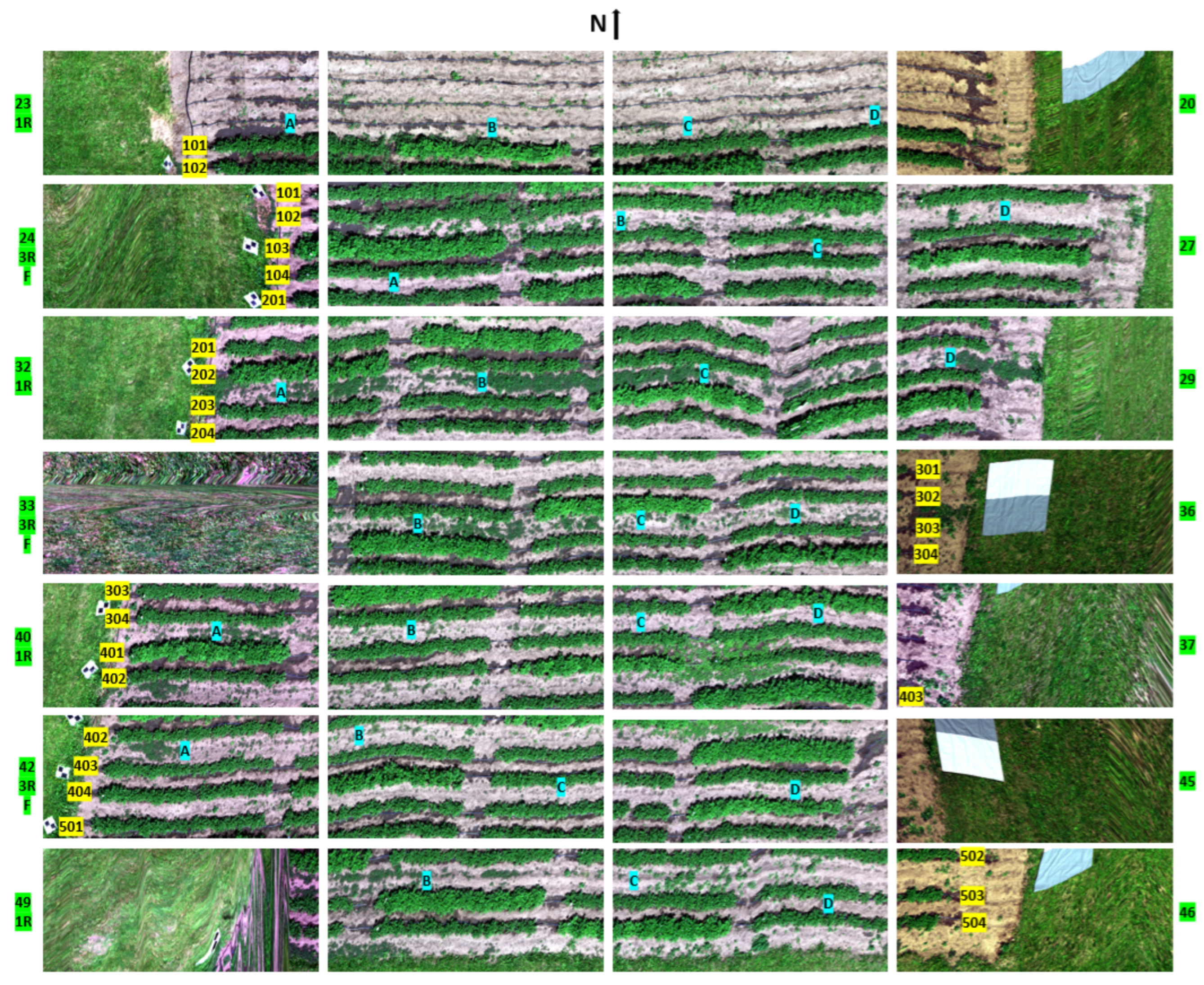
Figure 3.
The relevant hyperspectral images were manually put together to recreate the field layout [
14]. Due to the technical failure in the magnetometer of the camera, the images could not be geo-rectified. Hence, for the manual arrangement of the field layout, the images needed to be flipped and rotated to match the original layout of the field and account for the flight direction. The block numbers starting from 101 to 504 and the row plots A, B, C, and D are labeled for reference. The numbers in green on both sides of the figure represent the image numbers, and the letters F and R stand for flipped and rotated. A calibration tarp can be seen in a few of the images; however, we used downwelling irradiance sensor data for the reflectance calibration of the images.
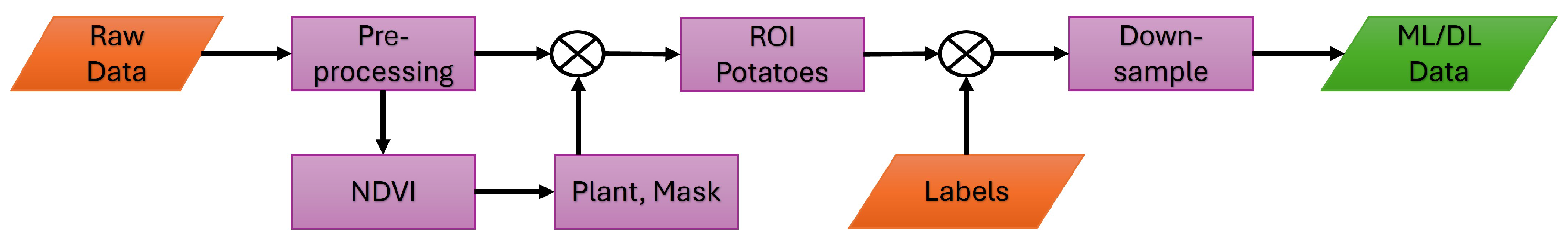
Figure 4.
Steps followed in this work to process the raw data before ML-DL analysis.
Figure 4.
Steps followed in this work to process the raw data before ML-DL analysis.
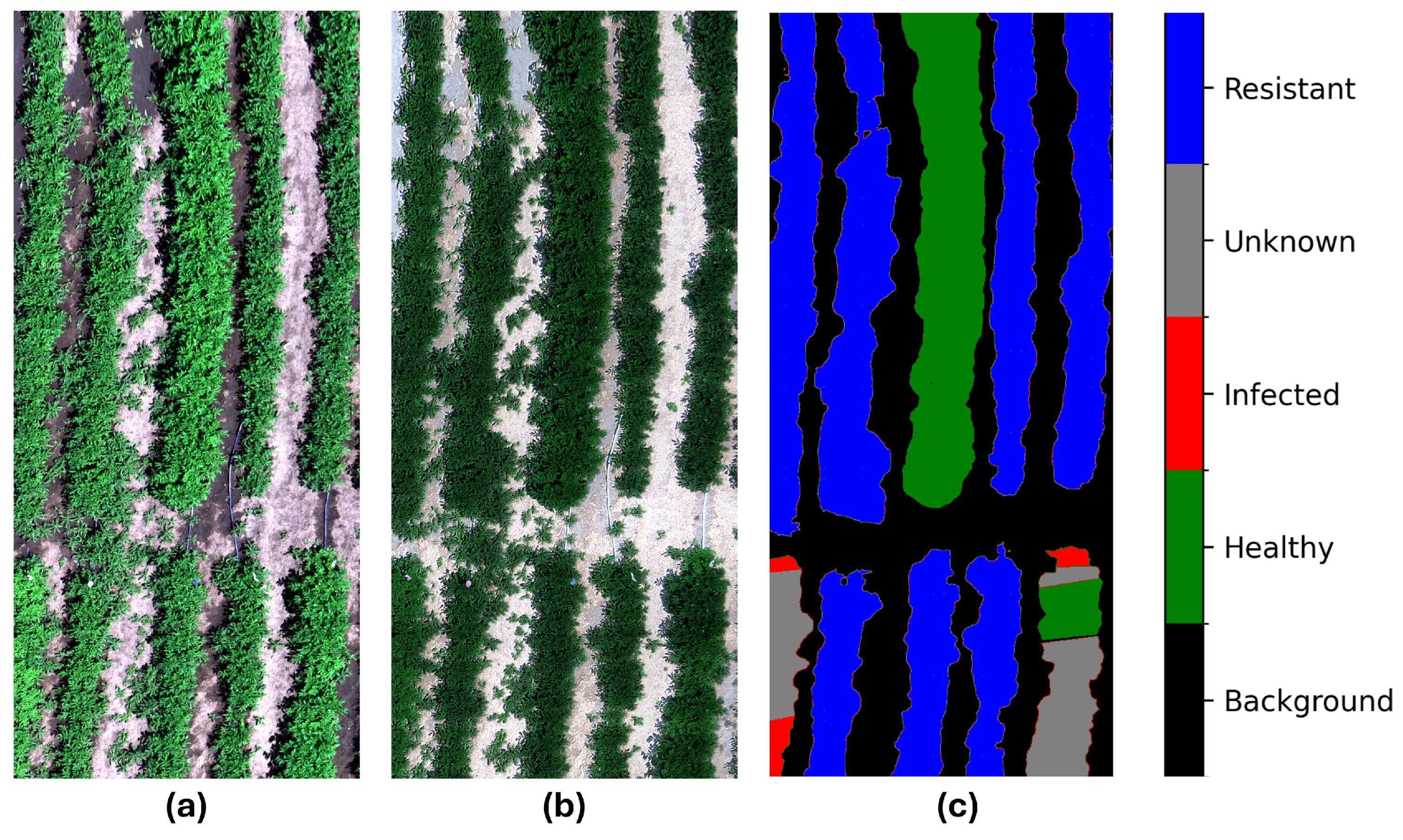
Figure 5.
True color (red: 639.8 nm, green: 550.00 nm, blue: 459.7 nm) representation of the (a) raw data; (b) processed data for a sample hyperspectral image; and (c) the respective ground truth labels of the image. The raw data are captured by the camera, and the processed data are radiance and reflectance calibrated, and finally normalized. The label contains background, healthy, and infected plants—these plots are susceptible to PVY; resistant—these plots are resistant to PVY; and the unknown labels, meaning the unknown status of PVY.
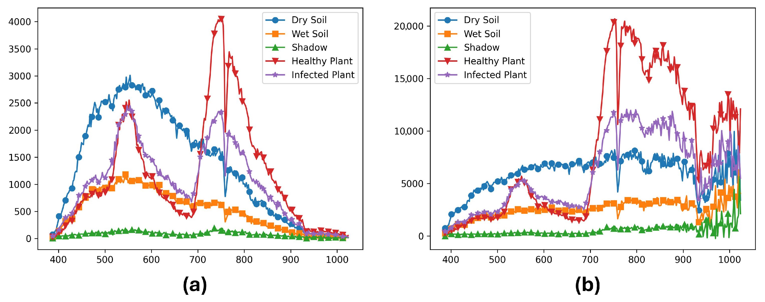
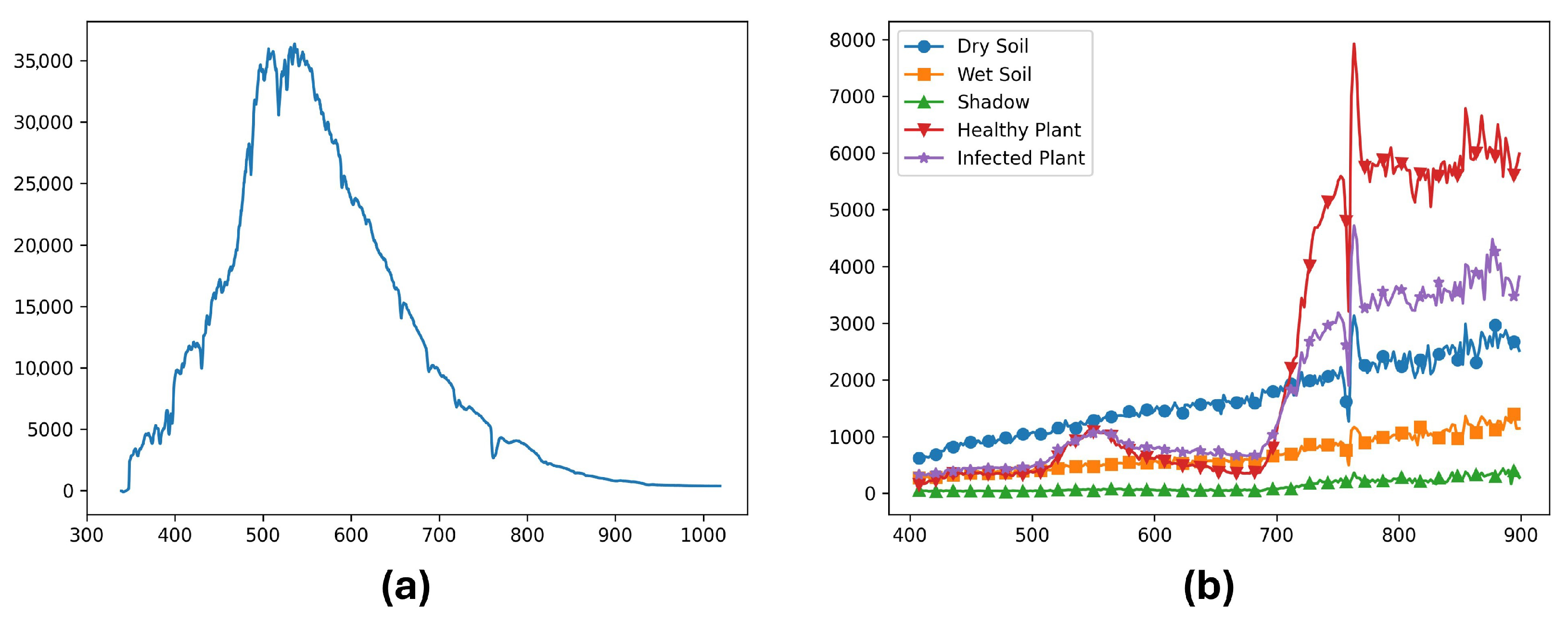
Figure 6.
(a) Raw data and (b) Radiance calibrated data for dry soil, wet soil, shadow, healthy plant, and infected plants from the same sample image. The x axis represents the wavelengths in nanometers, and the y axis represents (a) digital numbers (DN) produced by the camera, and (b) physical units of microFlicks (W/m2.sr.nm) (power per unit solid angle per unit area).
Figure 7.
(a) Downwelling spectra used for reflectance calibration, and (b) Reflectance calibrated data for dry soil, wet soil, shadow, healthy plant, and infected plants from the same sample image. The x axis represents the wavelengths in nanometers, and the y axis represents (a) downwelling irradiance physical units W/m2/nm, and (b) the unitless ratio of reflectance value multiplied by 10,000.
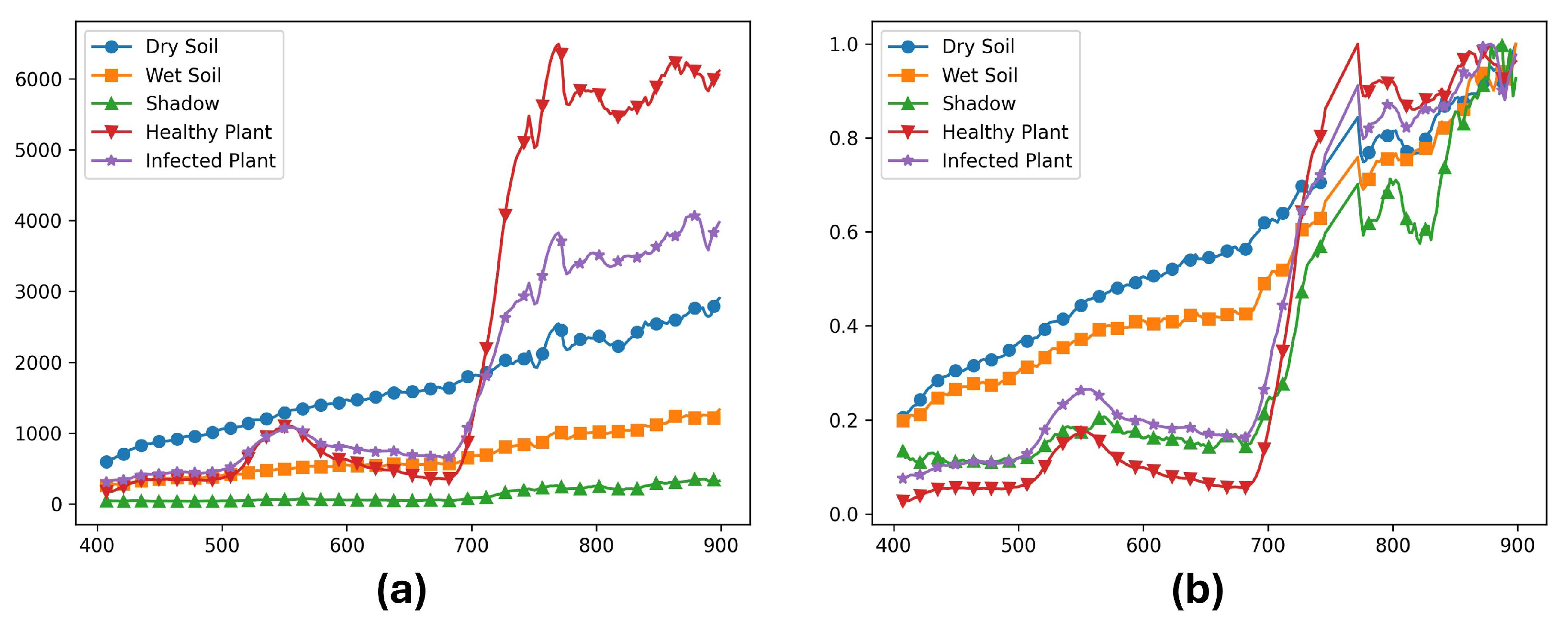
Figure 8.
(a) Smoothed reflectance data using the Savitzky–Golay filter and (b) Normalized reflectance data for dry soil, wet soil, shadow, healthy plant, and infected plants from the same sample image. Note that the bad bands are discarded in the plots. The x axis represents the wavelengths in nanometers and the y axis represents (a) the unitless ratio of reflectance values multiplied by 10,000, and (b) the normalized reflectances ranging from 0 to 1.
Figure 9.
Workflow diagram showing the steps involved in preparing the data for the ML/DL analyses. For the preprocessing steps, refer to
Figure 4.
Figure 9.
Workflow diagram showing the steps involved in preparing the data for the ML/DL analyses. For the preprocessing steps, refer to
Figure 4.
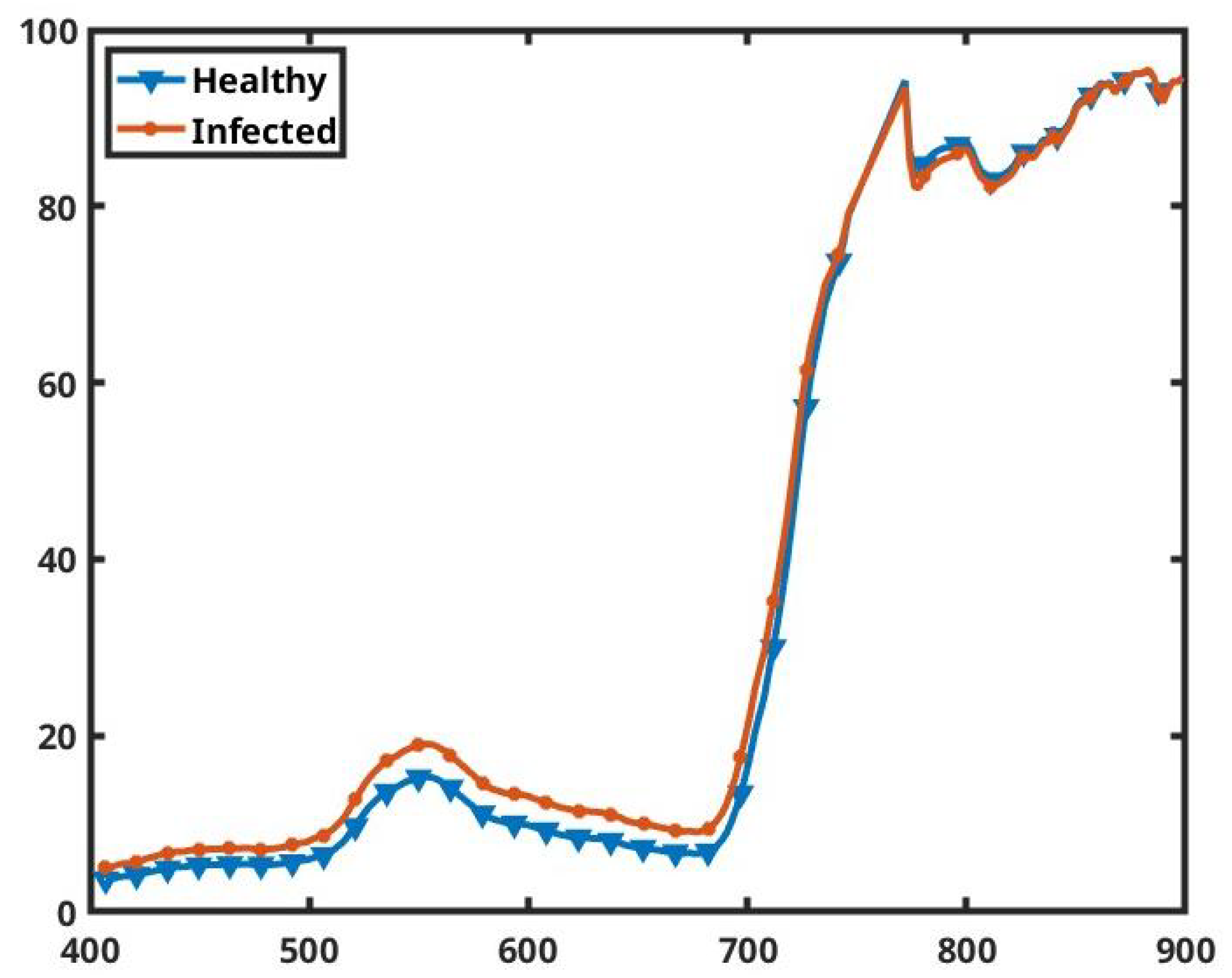
Figure 10.
The average spectra for all the healthy and infected pixels of the prepared dataset. The x axis represents the wavelengths in nanometers and the y axis shows the percentage of reflectance.
Figure 10.
The average spectra for all the healthy and infected pixels of the prepared dataset. The x axis represents the wavelengths in nanometers and the y axis shows the percentage of reflectance.
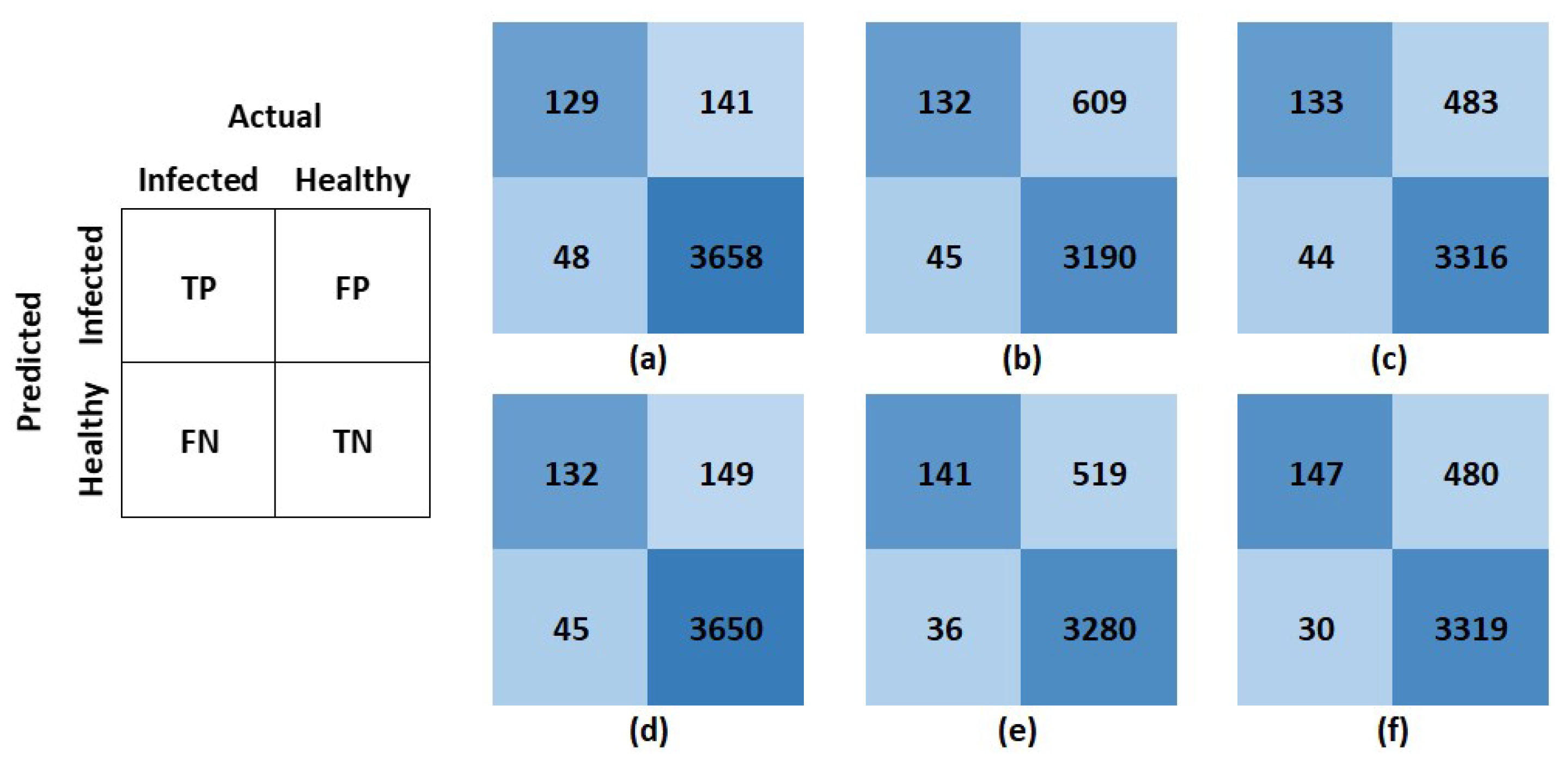
Figure 11.
The left figure shows the general structure followed for the confusion matrices presented herein. TP stands for true positive, FP for false positive, FN for false negative, and TN for true negative. In the matrices, rows represent predicted values, and columns represent actual values. Confusion matrices for (a) support vector machine, (b) decision tree, (c) K-nearest neighbors, (d) logistic regression, (e) feedforward neural network, and (f) convolutional neural network. The respective models report these confusion matrices on the unseen susceptible test set with normalization.
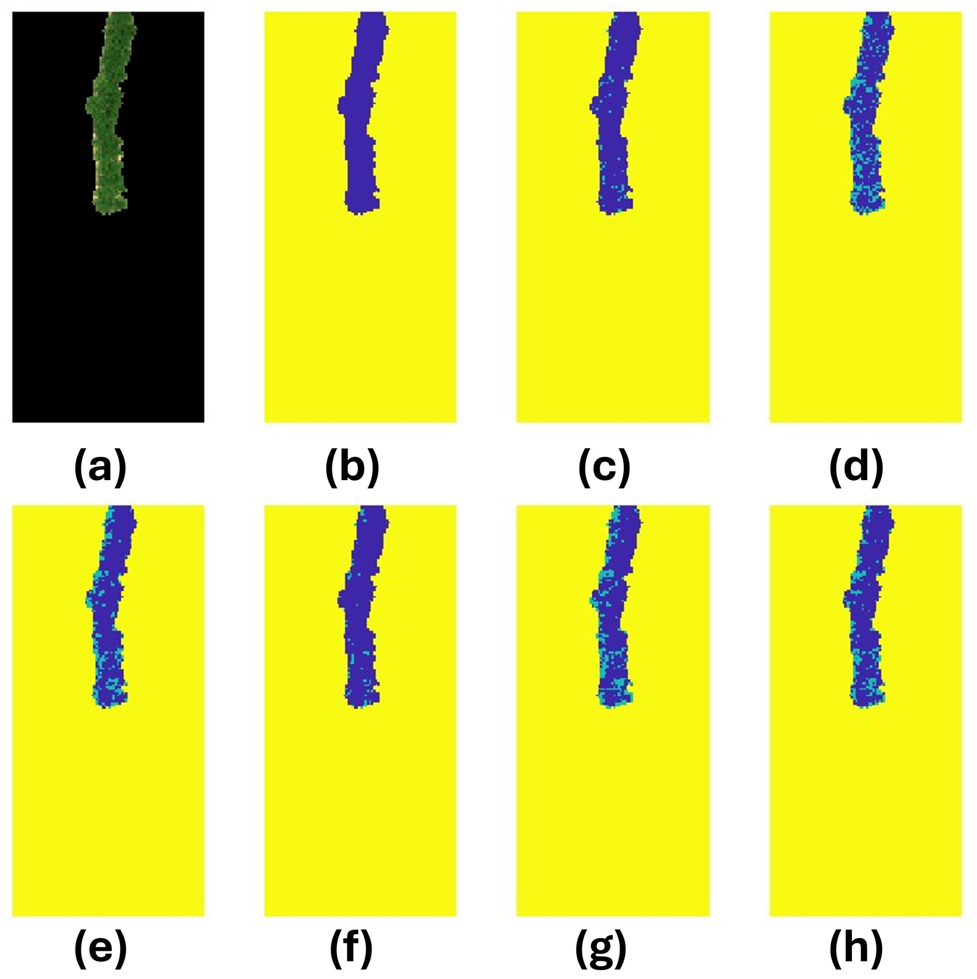
Figure 12.
Exploration of model performances on Image 39 of the test set. (a) RGB representation of the image after carefully curating the susceptible potatoes. (b) True labels of the PVY status for the image. Blue is healthy, green is infected, and yellow is the background. There are 66 known infected pixels in the image shown in green. The following subplots are the predictions of image 31 using the following models: (c) Support vector machine; (d) Decision tree; (e) K-nearest neighbors; (f) Logistic regression, (g) Feedforward neural network; and (h) Convolutional neural network.
Figure 13.
Exploration of model performances on Image 43 of the test set. (a) RGB representation of the image after carefully curating the susceptible potatoes. (b) True labels of the PVY status for the image. Blue is healthy, green is infected, and yellow is the background. There are no known infected pixels in the image, as shown in the true labels. The following subplots are the predictions of image 43 using the following models: (c) Support vector machine, (d) Decision tree, (e) K-nearest neighbors, (f) Logistic regression, (g) Feedforward neural network, and (h) Convolutional neural network.
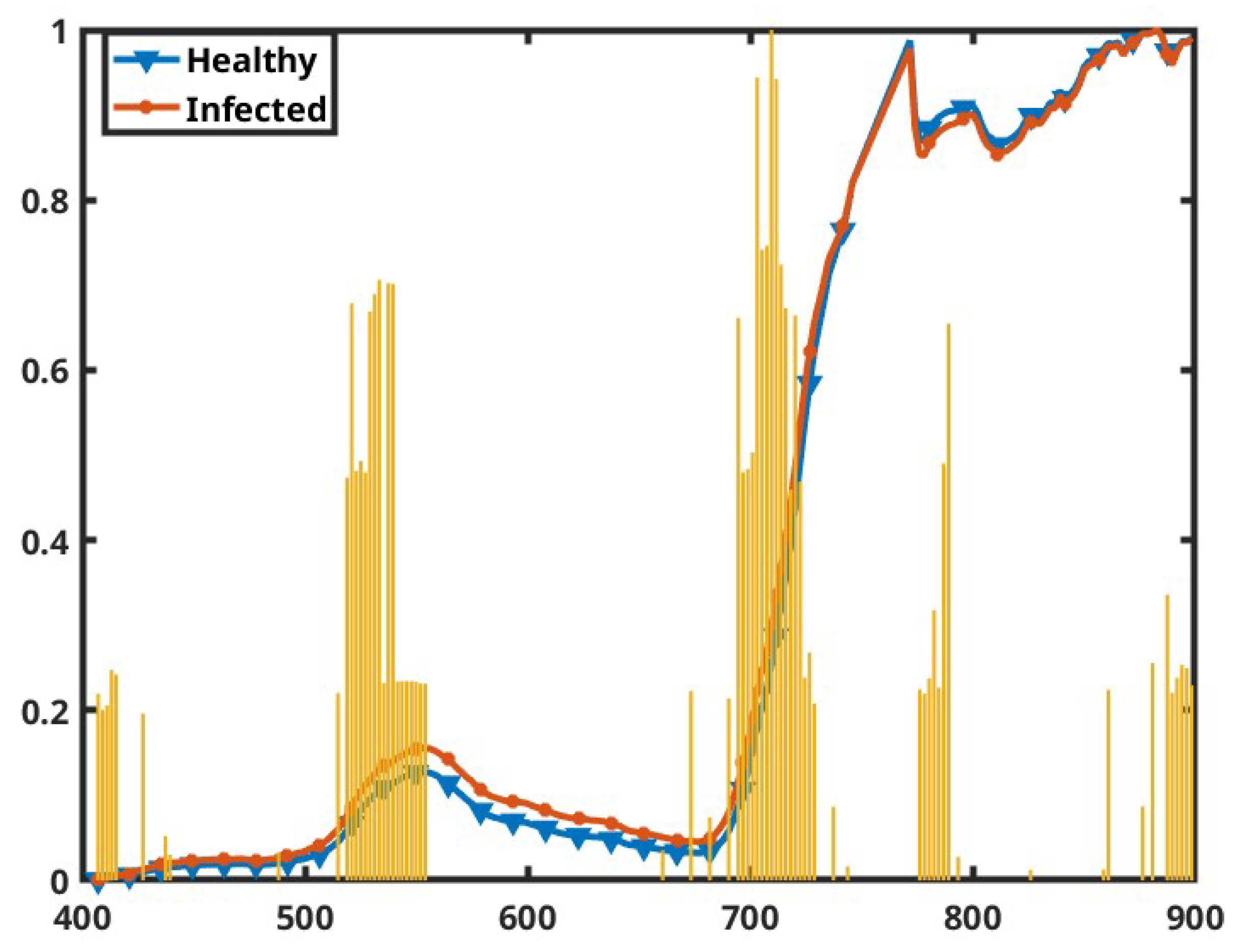
Figure 14.
Most relevant bands across the spectra shown in the yellow bar graphs. The line plots are the normalized mean spectra of the healthy and infected plants, as indicated by the color legends, shown for reference. The x axis represents the wavelengths in nanometers, and the y axis represents the normalized scale from 0 to 1.
Table 1.
Treatment descriptions across the field for all five blocks of the experimental field. This is important to help facilitate the tracking of the virus spread. T# represents the treatment used in the specific plots as mentioned in each of the rows.
Table 1.
Treatment descriptions across the field for all five blocks of the experimental field. This is important to help facilitate the tracking of the virus spread. T# represents the treatment used in the specific plots as mentioned in each of the rows.
| Treatment | Block 100 | Block 200 | Block 300 | Block 400 | Block 500 |
|---|
| T1—50% PVY | 104 D | 201 B | 302 C | 401 A | 504 C |
| T2—PVY + plants, PVY− Tubers | 101 B | 203 C | 301 A | 402 C | 501 D |
| T3—Uma control | 103 A | 204 D | 303 B | 404 D | 503 B |
| T4—DRN control | 102 C | 202 A | 304 D | 404 B | 502 A |
Table 2.
Summary of the training and testing datasets used in this study, including the number of images, downsampled hyperspectral pixels, number of infected pixels, and class distribution. Pixel counts are grouped into resistant and susceptible plots (total pixels), with the number of infected pixels reported from the susceptible subset. The ratio of infected pixels is calculated with respect to the total number of pixels.
| Dataset | Images | Total Pixels | Susceptible | Infected | Infected Ratio (%) |
|---|
| Training | 15 | 72,819 | 19,868 | 1617 | 0.081 |
| Testing | 4 | 23,364 | 3976 | 177 | 0.045 |
| Total | 19 | 96,183 | 23,844 | 1794 | 0.075 |
Table 3.
Classification results of support vector machine (SVM), decision tree (DT), K-nearest neighbors (KNN), logistic regression (LR), feedforward neural network (FNN), and convolutional neural network (CNN) on the test set. The model was trained and tested both with and without normalization on the susceptible data. The performance metrics evaluated are accuracy (Acc), precision (Prec), recall (Rec), and F1 score (F1). The best result for each of the metrics is shown in bold.
| With Normalization | Without Normalization |
|---|
| Model | Acc | Prec | Rec | F1 | Acc | Prec | Rec | F1 |
|---|
| SVM | 0.953 | 0.478 | 0.729 | 0.577 | 0.950 | 0.462 | 0.746 | 0.570 |
| DT | 0.836 | 0.178 | 0.746 | 0.288 | 0.743 | 0.116 | 0.718 | 0.199 |
| KNN | 0.868 | 0.216 | 0.751 | 0.335 | 0.898 | 0.268 | 0.746 | 0.395 |
| LR | 0.951 | 0.470 | 0.746 | 0.576 | 0.936 | 0.391 | 0.768 | 0.518 |
| FNN | 0.860 | 0.214 | 0.797 | 0.337 | 0.958 | 0.547 | 0.294 | 0.382 |
| CNN | 0.872 | 0.234 | 0.831 | 0.366 | 0.955 | 0.495 | 0.599 | 0.542 |
Table 4.
Classification results of support vector machine (SVM), decision tree (DT), K-nearest neighbors (KNN), logistic regression (LR), feedforward neural network (FNN), and convolutional neural network (CNN) on the test set. The model was trained on the susceptible data with and without normalization, and tested on the combined set of resistant and susceptible plants. The performance metrics evaluated are accuracy (Acc), precision (Prec), recall (Rec), and F1 score (F1). The best result for each of the metrics is shown in bold.
| With Normalization | Without Normalization |
|---|
| Model | Acc | Prec | Rec | F1 | Acc | Prec | Rec | F1 |
|---|
| SVM | 0.882 | 0.047 | 0.746 | 0.088 | 0.822 | 0.031 | 0.746 | 0.060 |
| DT | 0.668 | 0.017 | 0.746 | 0.033 | 0.640 | 0.015 | 0.718 | 0.030 |
| KNN | 0.707 | 0.019 | 0.757 | 0.038 | 0.775 | 0.025 | 0.746 | 0.048 |
| LR | 0.857 | 0.037 | 0.723 | 0.071 | 0.749 | 0.023 | 0.768 | 0.044 |
| FNN | 0.768 | 0.026 | 0.808 | 0.050 | 0.969 | 0.078 | 0.294 | 0.124 |
| CNN | 0.715 | 0.022 | 0.831 | 0.042 | 0.932 | 0.065 | 0.599 | 0.118 |
Table 5.
Classification results of support vector machine (SVM), decision tree (DT), K-nearest neighbors (KNN), logistic regression (LR), feedforward neural network (FNN), and convolutional neural network (CNN), evaluated on a test set solely consisting of resistant varieties with no infected samples. Models were trained on susceptible data, both with and without normalization. Since there are no infected samples in the test set, the ideal behavior is to classify all pixels as healthy. Accuracy (Acc) is reported. Precision (Prec), recall (Rec), and F1 score are omitted here, as all models yield 0 true positives (TP), making recall and F1 undefined, and precision equal to 0.
| Model | Acc with Normalization | Acc Without Normalization |
|---|
| SVM | 0.867 | 0.795 |
| DT | 0.633 | 0.618 |
| KNN | 0.673 | 0.750 |
| LR | 0.836 | 0.710 |
| FNN | 0.749 | 0.971 |
| CNN | 0.679 | 0.927 |
Table 6.
Prediction analysis of different ML-DL models on the test sets. The table shows the accuracy for each of the models on the images, along with the number of known infected pixels (# true infected), the number of predicted infected pixels by the trained model (# predicted infected), and the number of correctly identified infected pixels (# correct infected).
| Image | Model | Accuracy | # True Infected | # Predicted Infected | # Correct Infected |
|---|
| 26 | SVM | 0.942 | 54 | 42 | 38 |
| DT | 0.820 | 80 | 36 |
| KNN | 0.887 | 61 | 38 |
| LR | 0.928 | 51 | 40 |
| FNN | 0.901 | 56 | 38 |
| CNN | 0.910 | 69 | 46 |
| 31 | SVM | 0.935 | 57 | 49 | 26 |
| DT | 0.875 | 111 | 32 |
| KNN | 0.893 | 92 | 30 |
| LR | 0.928 | 55 | 26 |
| FNN | 0.899 | 101 | 37 |
| CNN | 0.892 | 103 | 35 |
| 39 | SVM | 0.963 | 66 | 119 | 65 |
| DT | 0.885 | 233 | 64 |
| KNN | 0.902 | 209 | 65 |
| LR | 0.968 | 113 | 66 |
| FNN | 0.890 | 230 | 66 |
| CNN | 0.887 | 234 | 66 |
| 43 | SVM | 0.954 | 0 | 60 | 0 |
| DT | 0.759 | 317 | 0 |
| KNN | 0.807 | 254 | 0 |
| LR | 0.953 | 62 | 0 |
| FNN | 0.792 | 273 | 0 |
| CNN | 0.832 | 221 | 0 |


