Article

An Ultra-Wide Swath Synthetic Aperture Radar Imaging System via Chaotic Frequency Modulation Signals and a Random Pulse Repetition Interval Variation Strategy

1
The Department of Space Control and Communication, Space Engineering University, Beijing 102249, China
2
The School of Information Science and Engineering, Southeast University, Nanjing 214135, China
3
The 15th Research Institute of China Electronics Technology Corporation, Beijing 100083, China
*
Author to whom correspondence should be addressed.
Remote Sens. 2025, 17(10), 1719; https://doi.org/10.3390/rs17101719
Submission received: 17 April 2025 / Revised: 1 May 2025 / Accepted: 13 May 2025 / Published: 14 May 2025
(This article belongs to the Section Engineering Remote Sensing)

Abstract

:
Ultra-wide swath synthetic aperture radar (SAR) systems are of great significance for applications such as terrain measurement and ocean monitoring. In conventional SAR systems, targets echo from the near-range and far-range of an observed swath mutually overlap, and the blind ranges are caused by those that the radar cannot receive while it is transmitting. Therefore, the swath of conventional SAR systems is limited due to their range ambiguity as well as the transmitted pulse blockage. With the development of waveform diversity, range ambiguity can be suppressed by radar waveform design with a low-range sidelobe without increasing the system’s complexity when compared to the scan-on-receive (SCORE) based on digital beamforming (DBF) technique. Additionally, by optimizing the pulse repetition interval (PRI) variation strategy, the negative impact of blind range on imaging can be reduced. Based on these technologies, this paper proposes a theoretical architecture to achieve an ultra-wide swath SAR imaging system via chaotic frequency modulation (FM) signals and a random pulse repetition interval variation strategy without increasing the antenna area. By transmitting time-variant chaotic-FM signals, the interference between targets in the near range and far range can be reduced by the corresponding match filters. Furthermore, random pulse repetition intervals increase the irregularity and aperiodicity of the blind ranges to further improve the imaging quality. Simulation results demonstrate that the proposed wide-swath SAR system has better performance compared to classical SAR systems.

1. Introduction

Synthetic aperture radar (SAR) is an active microwave sensor that can achieve observation all day in all weather conditions [1]. High resolution and wide swath are both of great importance in improving SAR observation efficiency in applications such as terrain measurement and ocean monitoring [2,3,4]. However, according to minimum antenna area constraints, wide unambiguous swath coverage and high azimuth resolution are contradicting requirements in SAR system design. Specifically, conventional single-channel SAR systems, such as ScanSAR [5] or terrain observation by progressive scans (TOPS) [6], achieve an ultra-wide swath at the expense of low azimuth resolution or degraded imaging quality.
To achieve an ultra-wide range swath in a high-resolution SAR system, the echo of scatterers at far ranges and near ranges should be distinguishable. Constrained by the pulse repetition interval (PRI) selected within a specific range, the echo duration of the observed swath exceeds one PRI so that the current raw data of near-range scatterers mutually interfere with the previous ones of far-range scatterers in the observed swath, which is the cause of range ambiguity. Digital beamforming (DBF) on receipt [7,8,9] is a technique for wide swath imaging which steers a narrow receiving beam to the direction according to the echo arrival time, while its limitation is that a very long antenna is required for the system. Orthogonal frequency division multiplexing (OFDM) signals have been studied for unambiguous wide-swath imaging in a multiple-input multiple-output (MIMO) configuration, and the imaging quality is degraded by the cross-correlation energy of the waveforms, especially in the actual case of a distributed scatter scenario [10,11,12,13]. These technologies increase the system complexity that is structured by multiple aperture antennae.
Inspired by waveform diversity [14,15], radar waveform design has the potential to achieve low-range sidelobe and further suppress range ambiguity while not increasing the system complexity. After transmitting the designed waveforms during different PRIs, radar echoes of different range intervals can be separated by the corresponding match filters. The maximum unambiguous range can be extended by increasing the waveform number. Therefore, a low sidelobe radar waveform family with a larger waveform number has the promise to achieve an ultra-wide swath in the high-resolution imaging system. Currently, the waveforms based on up–down chirps [16,17,18], piecewise nonlinear frequency modulation (NLFM) waveforms [19,20], and NLFM waveforms using Fourier series [21,22] increase the waveform diversity to achieve low-range sidelobe and further range ambiguity. However, this series of deterministic waveform modulations has a tradeoff between the waveform properties of a low sidelobe and uncorrelation, so the limited number of waveforms restricts the low sidelobe performance. To achieve an ultra-wide swath by further suppressing the range ambiguity, the time–frequency relationships of the waveforms need to be designed as diversely as possible to improve the uncorrelation. The use of chaotic systems in waveform design has been proposed previously and has the potential to achieve high resolution with low sidelobe [23,24,25]. Specifically, uncorrelated chaotic frequency modulation (FM) waveforms can be generated in large quantities, which is beneficial to suppressing range ambiguity, thus providing feasibility for a wide swath SAR system design.
To obtain a continuous ultra-wide swath, the PRI needs to be designed, since it determines the distribution of the blind ranges and further impacts the imaging performance. Due to the occlusion between transmitting and receiving, blind strips in the imaging swath will occur with a constant PRI. The existing PRI variation strategy includes the linear PRI variation [26,27,28] and the optimized PRI variation strategy [29,30,31,32,33]. The linearity of the PRI variation leads to the regular distribution of the lost pulses so that high sidelobes are present in the vicinity of the mainlobe. In particular, one blockage may cause local sub-Nyquist sampling with low oversampling and result in lower local information density and more challenging blockage recovery. To overcome the issue caused by the regularity or even periodicity of linear variation sampling, a series of optimized PRI variation strategies are proposed [29,30,31,32,33] to improve the reconstructed performance. Inspired by these optimized PRI variation strategies, the imaging performance has the potential to be further improved by introducing more irregularity and aperiodicity in PRI variation strategies.
This paper proposes an ultra-wide swath imaging SAR system based on chaotic FM signals. The cores of this system utilize chaotic FM signals as transmitted pulses and randomize the pulse repetition interval. By transmitting chaotic FM signals, adjacent transmitted pulses have weak cross-correlation, which means that the far-range return pulses do not interfere with those aliased near-range return pulses after pulse compression. By randomizing the pulse repetition interval, the blind range caused by the occlusion of the transmitting pulse is distributed throughout the entire width, avoiding the inability to receive echoes at specific ranges. Combining time-domain range migration correction and sparse Bayesian learning (SBL) along azimuth, the scattering information of the scene can be reconstructed, thus achieving high-resolution wide-swath imaging.
Overall, the main contributions of this paper are presented as follows:
(1)
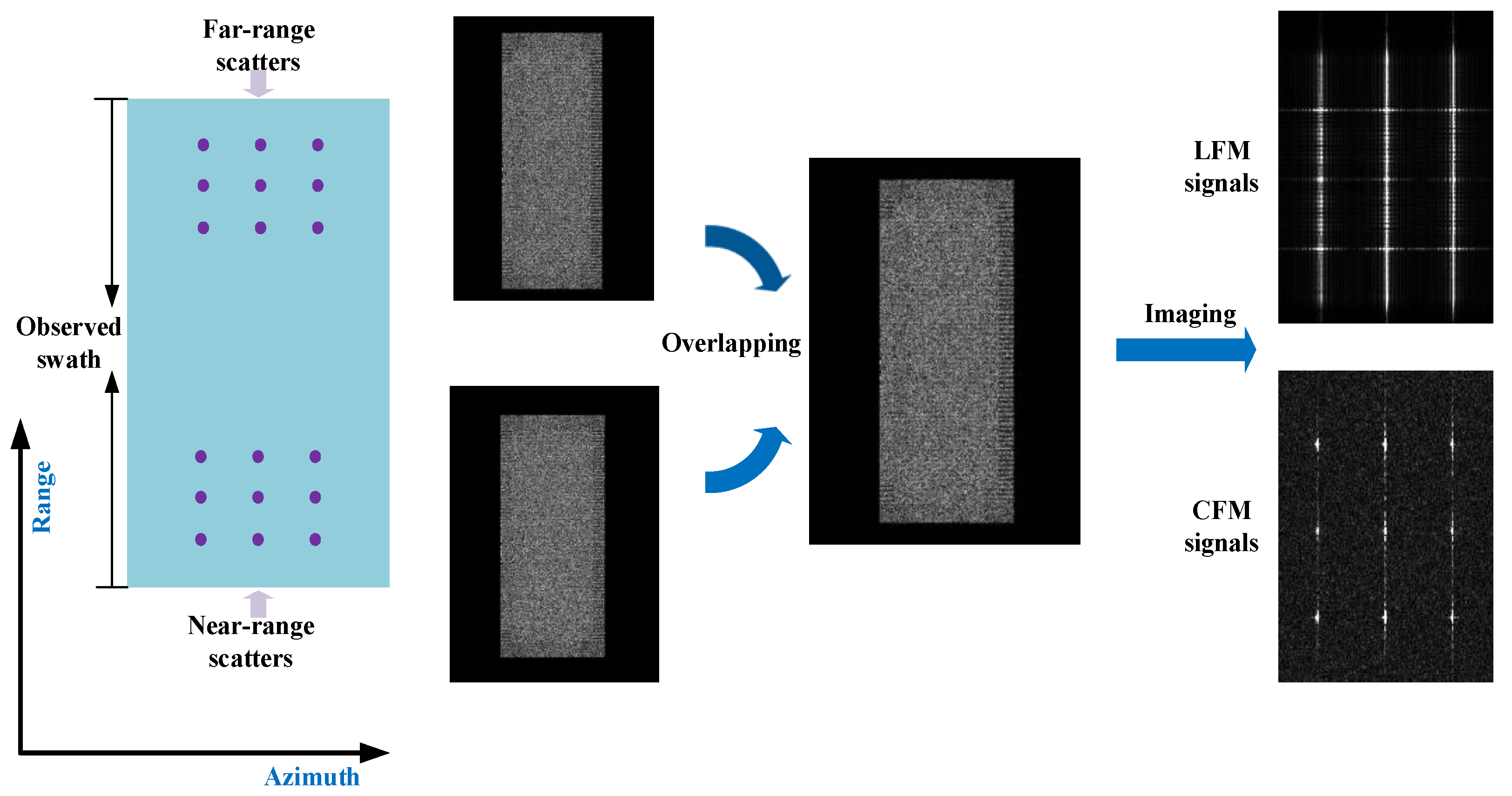
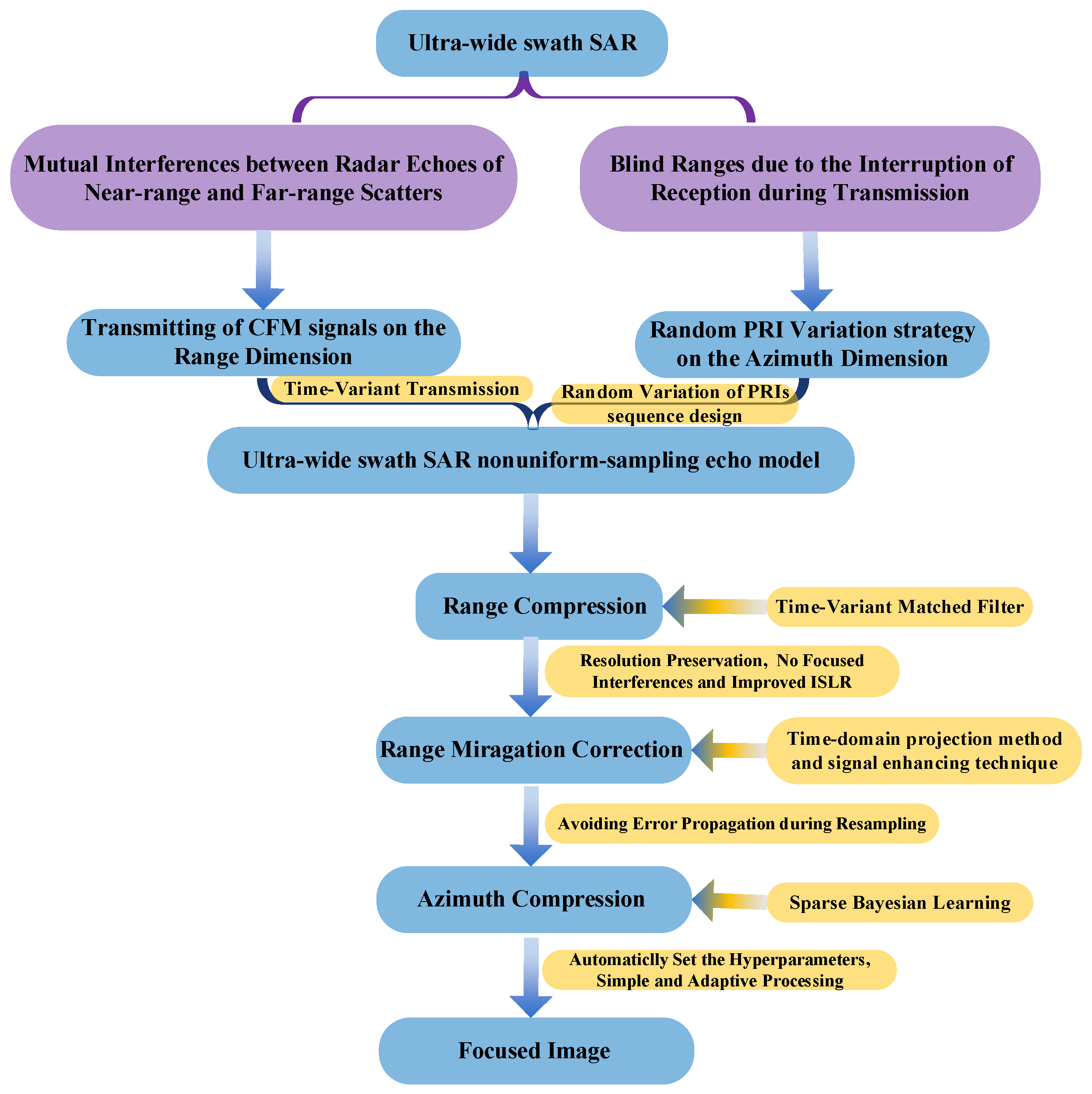
Replacing the chirp signal, chaotic FM signals are transmitted to avoid mutual interferences from the raw data of near-range and far-range scatters to achieve ultra-wide swath observation. Chaotic FM signals are time-variant transmitting signals and have different matched filters so that the raw data of near-range and far-range scatters after signal processing avoid mutual interferences in ultra-wide imaging. The alternative, transmitting signals, brings superior imaging performance with an improved mean peak sidelobe ratio (PSLR) and preserved resolution, assuming that the chaotic map obeys the uniform distribution.
(2)
An optimized random PRI variation strategy is proposed to keep the PRI variation nonlinear so that the blind ranges are discontinuously and nonuniformly distributed on the whole swath. To achieve azimuth focusing under nonuniform sampling, a reconstruction algorithm based on the sparsity Bayesian learning (SBL) is proposed in the optimized random PRI variation strategy. After range compression based on the matched filtering (MF) method, range cell migration correction (RCMC) is accomplished by interpolating and summing up. During the RCMC, an innovative back-projection technique is adopted to achieve signal enhancement. Instead of resampling the nonuniform sampling signal into a uniform grid, an observation model is established and reconstructed using SBL to achieve azimuthal compression. Our proposed sampling strategy and reconstruction algorithm take full advantage of nonuniform sampling to suppress the high sidelobes due to the periodicity of the lost pulses and improve reconstruction performance under low oversampling or even sub-Nyquist sampling.
The remainder of this paper is organized as follows. Section 2 introduces the limitations of the conventional SAR system, proposes an ultra-wide swath SAR system using chaotic FM signals with a random PRI variation strategy, and details the imaging processing of the proposed system. Section 3 consists of simulation experiments based on point targets and extended targets. In Section 4, a discussion is given to show the performance and advantages of our proposed system. Section 5 concludes this paper.

2. Materials and Methods

Firstly, the limitations of the conventional SAR system are introduced in this section. Then, we propose an ultra-wide swath SAR system using chaotic FM signals with a random PRI variation strategy. Lastly, we give the imaging processing algorithm of the proposed ultra-wide swath SAR system.

2.1. Limitation of Conventional SAR Systems

A conventional SAR system transmits linear frequency-modulated (LFM) pulses with constant pulse repetition interval (PRI), and the echo can be written as follows [1]:
s c t , η = x i , y i σ i W i t , η exp j π K r t 2 R i η / c 2 exp j 4 π R i η λ + n t , η
where t and η are the fast time along the range and the slow time along the azimuth, respectively. R i η represents the range between radar and the point target located at the coordinate x i , y i at azimuth time η , where x i and y i denote the azimuth and range coordinates, respectively. σ i and W i t , η are the radar cross-section and the weighting pattern corresponding to the target at x i , y i . K r denotes the chirp rate of LFM signals, c is the light speed, λ is the wavelength, and n t , η is the system noise.
When designing SAR systems, it is usually assumed that echoes of the imaging swath are received between two adjacent transmitted pulses. The limitation of swath width can be expressed as
W < c / 2 P R I / sin θ
where θ is the incident angle. If the swath is wider than c / 2 P R I / sin θ , range ambiguity should be considered. Specifically, the echo of the current pulse of a target located at R 1 is aliased with the echo of the previous pulse of a target located at R 2 = R 1 + c / 2 P R I . Since the pulses share the same range frequency modulation rate K r , interference will occur at both ranges after range compression. Another issue to be solved is blind range, which means for each transmitted pulse whose width is ι 0 , the echoes of targets at
p P R I c 2 R p P R I + ι 0 c 2 , p = 0 , 1 , 2 ,
will not be received because the radar cannot receive while transmitting, resulting in blind strips in the imaging result [26,27].

2.2. Ultra-Wide Swath SAR System Via Chaotic FM Signals and a Random PRI Variation Strategy

To solve the range ambiguity and blind range problem for wide swath observations, this section proposes an ultra-wide swath SAR system based on chaotic FM signals in the presence of a random PRI variation strategy.

2.2.1. Chaotic FM Signals

As mentioned in Section 2.1, range ambiguity occurs when the SAR system transmits pulses with the same FM rate. A possible way to suppress range ambiguity is to use time-variant chaotic FM signals as transmitted pulses. This subsection explains the feasibility by introducing the definition and the properties of chaotic FM signals, which is followed by the signal waveform design method for the proposed SAR system.
Chaotic FM signals are signals generated by modulating the frequency using chaotic sequences, which can be expressed as follows [34,35]:
s 0 t = exp j 2 π t ϕ τ ; c s q c 0 d τ
where ϕ t ; c s q c 0 is the instant frequency
ϕ t ; c s q c 0 = f 0 + K k = 0 M 1 c k g τ 0 t k τ 0 + τ 0
f 0 is the central carrier frequency. M and τ 0 are the subpulse number and the subpulse width, respectively. K is the frequency modulation coefficient of the chaotic FM signal. g τ 0 t is the unit pulse of duration τ 0 defined on 0 , τ 0 . c s q c 0 = c i i = 0 , 1 , , M 1 is the chaotic sequence defined as
c k + 1 = f c k
where f : 0.5 , 0.5 0.5 , 0.5 is a nonlinear mapping and c 0 is the initial state. Typical chaotic maps are listed in Table 1 of Reference [34]. The chaotic sequences are sensitive to the initial state [34], i.e., a slight change in c 0 can lead to approximately uncorrelated sequences. Thus, it can be inferred that, by designing chaotic sequences, uncorrelated adjacent chaotic FM pulses can be generated, which is beneficial to suppressing the range ambiguity of SAR systems.
In this paper, the Bernoulli map is chosen to generate chaotic FM signals due to the following reasons. First, the mainlobe width of the autocorrelation function is constant. The expression of the mainlobe of the autocorrelation function is as follows (details are shown in Appendix A):
χ τ M τ 0 sinc K τ , τ < τ 0
which means that the resolutions of the chaotic FM pulses after range compression are identical and equal to ρ r a n g e = c / 2 K , leading to the preservation of the range resolution of the proposed SAR system. Second, the Bernoulli map can be achieved using an analog circuit, which is beneficial to hardware implementation considering the precision and speed.
As mentioned in Section 2.1, range ambiguity occurs when the two adjacent pulses have the same waveform. In other words, the range ambiguity can be suppressed when the transmitted pulses are azimuth time-variant. As for chaotic FM pulses, this can be achieved by changing the initial state. The cross-correlation function (CCF) of chaotic FM pulses with the Bernoulli map is derived as follows (details are shown in Appendix B):
R c τ = + s 0 t s 1 t τ d t = M 1 τ 0 exp j 2 π K c k τ exp j 2 π K i = 0 k 1 c i 0 i = 0 k 1 c i 1 τ 0 , τ < τ 0 k = m M τ 0 exp j 2 π K τ m τ 0 c k exp j 2 π K i = 0 k c i 0 i = 0 k m c i 1 τ 0 , m 1 τ 0 < τ < m τ 0 , m 2
The CCF of a chaotic FM signal with the Bernoulli map is similar to random noise and has no obvious mainlobe compared to a chirp pulse. Figure 1 illustrates the matched filtering results of adjacent azimuth chaotic FM pulses and chirp pulses, respectively. False targets can be seen when chirp pulses are transmitted, while only the matched chaotic FM pulse is compressed, which demonstrates that range ambiguity can be suppressed when transmitting chaotic FM pulses.
To summarize, the chaotic FM signal with the Bernoulli map is chosen for the proposed ultra-wide swath SAR system. In order to preserve the range resolution, the frequency modulation coefficient K should be set as
K = c 2 ρ r a n g e

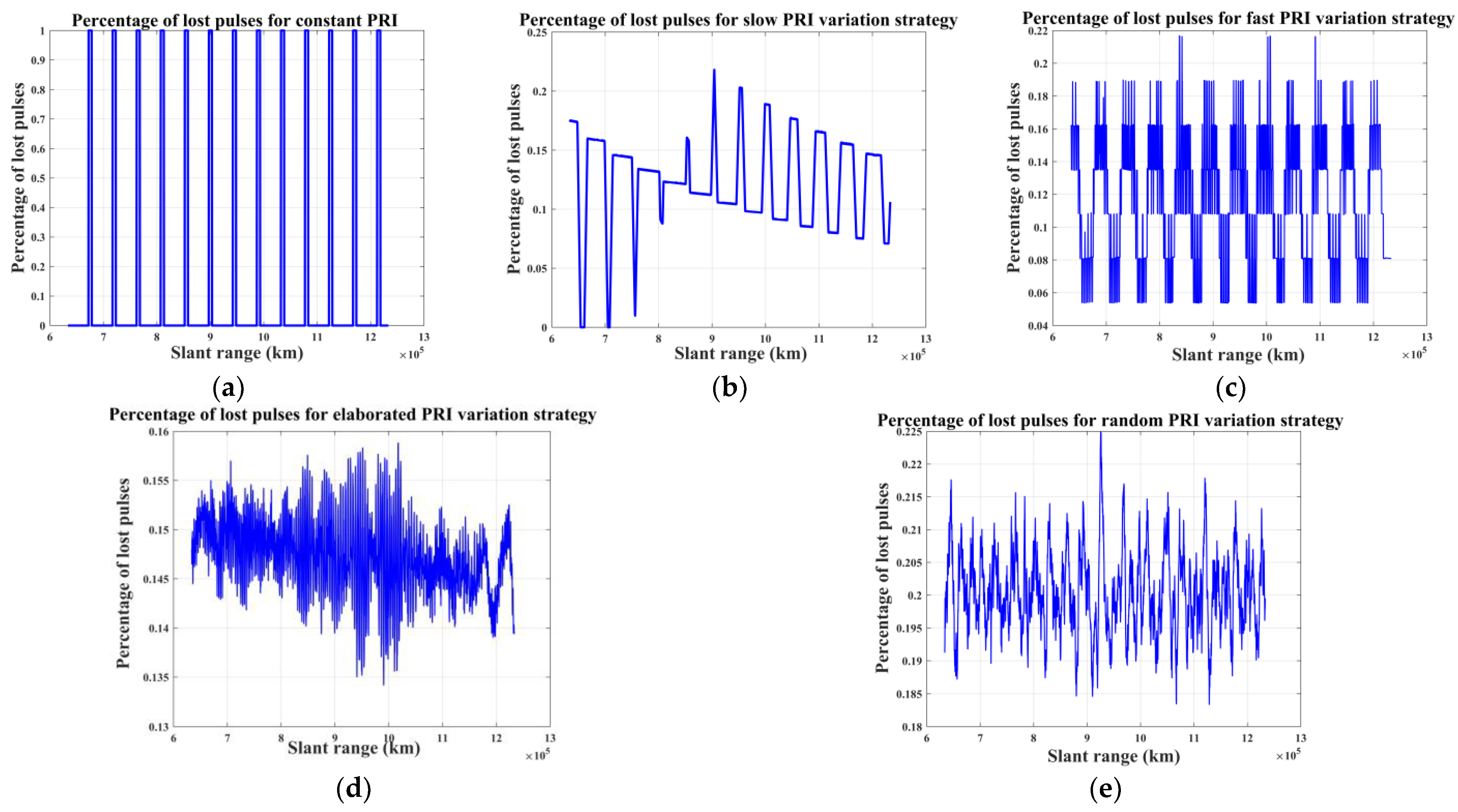
2.2.2. Random PRI Variation Strategy

Blind ranges locate at fixed slant range since the radar cannot receive while it is transmitting with constant PRI, as illustrated in Figure 2a. This drawback can be overcome by continuous variation in PRI along azimuth [26,27]. Currently, PRI variation strategies mainly include the slow linear PRI variation, the fast linear PRI variation, and the elaborated PRI variation [26,27]. The time delays of this nonuniform sampling are changed and the location of each lost pulse varies so that the blind ranges are shifted and distributed over the whole swath, as shown in Figure 2b–d. This strategy can control the location of the blind ranges in a straightforward way. Meanwhile, a series of optimized nonlinear PRI variation strategies have been proposed to improve blockage recovery and imaging performance after reconstruction [29,30,31,32,33].
Inspired by the optimized nonlinear PRI variation strategy and compressive sensing (CS) theory [36,37,38,39,40,41,42,43,44,45,46], this section further exploits the potential of nonuniform sampling, especially under low oversampling or even sub-Nyquist sampling, to overcome the blind ranges due to the interruption of reception during transmission and achieve gapless ultra-wide swath observation. The proposed random PRI variation strategy is demonstrated as follows. The PRIs can be randomly chosen as long as the minimum PRI and the maximum PRI are determined. Assuming that a sequence of N pulses with different PRIs are denoted by P R I n , n = 0 , 1 , , N 1 , each P R I n randomly varies between the maximum and the minimum of the PRIs, which are represented by P R I max and P R I max , respectively. The nth PRI is given as follows:
P R I n = r a n d P R I min , P R I max
where r a n d e , f represents the random variable range from e to f . As a proper PRI span Δ P R I = P R I max P R I min can ensure the sampling in the azimuth direction and does not significantly impact range and azimuth ambiguities, a reasonable principle to design sequences of PRIs is to choose the maximum PRI span so that blind ranges are almost uniformly distributed over the whole swath. P R I max should be kept small enough to avoid the azimuth spectrum aliasing:
P R I max ρ a / V e
where V e is the equivalent radar velocity and ρ a is the azimuth resolution. As the observed swath is ultra-wide and the processing method is based on CS theory, P R I min theoretically can be arbitrarily small. Because the actual SAR system needs to consider the duration of transmitting pulses, P R I min is at least larger than one pulse duration ι 0
P R I min ι 0
The random variable follows the Gaussian distribution. Figure 2e shows a simulated blind range of the PRI sequence with Gaussian random distribution. Compared with the linear PRI variation strategies, the distribution of blind range presents irregularity and conformity on the whole swath.
The design of this PRI sequence does not require high oversampling to avoid azimuth ambiguities, and the data rates are lower compared to the linear PRI variation. This nonuniform sampling method eliminates regularity and periodicity, and it avoids large gaps in the slow linear PRI variation and the tedious design in the fast linear PRI variation and the elaborated PRI variation.

2.2.3. System Analysis

This subsection analyzes the range impulse response of the proposed system.
(1)
System Performance after Range Compression
As the number of phasors increases, the amplitude of the autocorrelation function r = χ τ approximately follows the Rayleigh distribution [47,48]:
ρ r = 2 r / ( M m + 1 ) exp r 2 / ( M m + 1 )
So the mean value of the autocorrelation amplitude is τ 0 π M m + 1 / 2 0.886 τ 0 M m + 1 . Additionally, the phase of each vector follows the uniform distribution in the interval π , π with the previous parameter setting K τ 0 1 , and each vector is mutually independent. According to the law of large numbers, the phase of the autocorrelation function also follows the uniform distribution in the interval π , π .
The above analysis of system performance after range compression is concluded here: (a) In the mainlobe region, the amplitude and phase of the autocorrelation function do not vary with the initial state c 0 . When a subpulse number M is a large number and the chaotic map obeys the uniform distribution, the amplitude and phase of the autocorrelation function are approximately equal to M τ 0 sin c K τ and 0, respectively. (b) In the sidelobe region, the amplitude and phase of the autocorrelation function appear as stochastic behavior and approximately follow the Rayleigh distribution and uniform distribution, respectively. Statistical simulations are consistent with these inferences, as illustrated in Figure 3. The mean values of amplitude and phase are 0.886 τ 0 M m + 1 and 0, respectively. The autocorrelation function is influenced, but is not determined by, the initial state.
As illustrated in Figure 4, these chaotic FM signals are modulated by the chaotic sequences with the Bernoulli map at various initial states. The mainlobe region of the autocorrelation functions remains unchanged while it presents the stochastic feature in the sidelobe region.
(2)
Integral Sidelobe Ratio (ISLR) Performance Along Range After Azimuth Compression
Azimuth compression in SAR imaging is essentially a coherent superposition of transmitted signals after range compression. While the above analysis focuses on the characteristics of a single chaotic FM signal, the discussion on the superposition of multiple chaotic FM signals after autocorrelation is as follows. Assuming that N is the superposition number, the superposition of autocorrelation functions is given as
Σ χ τ = N M τ 0 sin c K τ , τ < τ 0 n = 1 N k = m M τ 0 exp j 2 π K c k n τ m τ 0 + i = k m + 1 k c i n τ 0 , m 1 τ 0 < τ < m τ 0 , m 2 0 , τ e l s e
where c k n is the k-th number of the n-th chaotic sequence. Correspondingly, the mainlobe and sidelobe regions present coherent and incoherent integration characteristics, respectively. In the mainlobe region, the superposition is the integration of multiple real numbers so that the amplitude increases by 20 l o g 10 N   dB and the phase is still 0. In the sidelobe region, the superposition of multiple autocorrelation functions is still the two-dimensional random walk with N M m + 1 steps alongside one autocorrelation function with M m + 1 steps, so the amplitude and phase of superposition approximately follow the Rayleigh distribution and uniform distribution, respectively. The mean values of the amplitude and phase are 0.886 τ 0 N M m + 1 and 0, respectively. And the mean value of the amplitude increases by 20 l o g 10 N d B . Therefore, ISLR after the superposition of multiple autocorrelation functions improves by
20 l o g 10 N 20 l o g 10 N = 10 l o g 10 N
This quantitative analysis result is confirmed by the simulation result in Figure 5. Assuming that one thousand chaotic FM signals with the same uniform map and different initial states are generated, the ISLR theoretically improves by 30   dB comparing them to that of a single autocorrelation function. The statistical ISLR in Figure 4 improves by 29.81   dB . The inference is approximately consistent with the numerical example.
To conclude, by adopting chaotic FM transmitted signals and a random PRI variation strategy, the proposed system suppresses range ambiguity and avoids the regularity of blind ranges to achieve gapless wide-swath observation.

2.3. Imaging Algorithm for the Proposed Ultra-Wide Swath SAR System

Since the proposed SAR system adopts random azimuth sampling, fast Fourier transform (FFT) along azimuth is not applicable, which means that imaging cannot be performed using a traditional method such as range-Doppler algorithm (RDA) or chirp scaling algorithm (CSA) [1]. This section introduces an imaging method for the proposed SAR system, which is suitable for both oversampling and undersampling conditions. The method consists of three steps, namely range compression, range cell migration correction (RCMC), and azimuth reconstruction.

2.3.1. Range Compression Based on Matched Filtering

The echo of the proposed SAR system can be expressed as
s c t , η = x i , y i σ i F i ( η ) W i t , η s 0 t 2 R i η / c exp j 4 π R i η / λ + n t , η
Matched filtering is achieved by convolution in the fast time domain, and the signal after range compression is
s r c t , η = x i , y i σ i F i ( η ) W i t , η χ t 2 R i η / c exp j 4 π R i η / λ + n t , η
where χ t is the autocorrelation function mentioned in Section III.

2.3.2. Time Domain RCMC for Random Sampling

Due to the random azimuth sampling of the proposed system, the echo cannot be transformed to a range-Doppler (RD) domain using FFT, which means RCMC cannot be implemented in the way RDA or CSA does. Inspired by the back projection algorithm, RCMC using azimuth time domain projection is presented as follows.
First, the scene is divided into P and Q grids along the range and azimuth, respectively. The grid length is set as slightly less than the system resolution. Secondly, for each range line, the signal after range compression is upsampled by zero-padding in the range frequency domain. The slant range from each grid of the imaging area to the radar at each azimuth sampling instant is calculated and used to find the complex amplitude of the echo signal in the upsampled signal. Denote the slant range and the extracted signal of the m-th grid at the k-th azimuth sampling instant as R k , m and y e x , k m , respectively, and the azimuth echo can be expressed as
Y e x t r a c t m = y e x , 1 m , y e x , 2 m , , y e x , N m T
Since the extracted echo contains clutter and noise, the signal is enhanced by (details are shown in Appendix C) the following:
Y e n h a n c e , m = A m A m H Y e x t r a c t m
A m = exp j 4 π R 1 , m λ exp j 4 π R 2 , m λ exp j 4 π R N , m λ N × 1
where Am is the projection vector and H denotes conjugate transpose operation.
Then, for each azimuth time instant, the enhanced signals of grids with the same nearest slant range are added together, and the sum is assigned to the corresponding imaging grid in the first step. After traversing all azimuth sampling instants, RCMC is completed, and the signal at a certain range cell is represented by
s c t 0 , η = x i , y i σ i W i t 0 , η F i ( η ) exp j 4 π R i η η c i λ + n t 0 , η
where η c i is the beam center crossing time for the target located at x i , y i .

2.3.3. Azimuth Reconstruction Based on SBL

After RCMC, the signal in each range cell can be expressed as the following observation model:
s N × 1 = D N × Q σ Q × 1 + n N × 1
where s N × 1 = [ s c t 0 , η 1 , s c t 0 , η 2 , , s c t 0 , η N ] T is the vectorized signal after range compression and RCMC. D N × Q = D i t 0 , η n n = 1 , i = 1 N , Q represents the mapping between the non-uniform received azimuth signal and the imaging grids, where D i t 0 , η n = F i η W i t 0 , η n N T r exp j 4 π R i η n η c i / λ . σ = σ 1 , σ 2 , , σ Q T is the vectorized backscattering cross-sections of targets in the same range gate. n N × 1 = n t 0 , η 1 , n t 0 η 2 , , n t 0 , η N T denotes the noise.
Due to the occlusion of the transmitting pulse, some of the echo signal may be missing, which may result in sub-Nyquist sampling. CS is used here for reconstructing the scene [36,37,38,39,40,41,42,43,44,45,46]. Signal sparsity is very important in CS reconstruction. Since the reconstruction of this proposed algorithm is performed on each range bin, those sparse methods for the entire image, such as edge-based curvelet transform, are no longer applicable. Considering the fluctuation of the one-dimensional signal of each range bin, the wavelet basis ψ Q × Q is selected here for sparse representation [49], that is σ Q × 1 = ψ Q × Q ρ Q × 1 , and the observation model can be converted to
s N × 1 = D N × Q ψ Q × Q ρ Q × 1 + n N × 1 = Θ N × Q ρ Q × 1 + n N × 1
where Θ N × Q = D N × Q ψ Q × Q .
SBL adopts the relevance vector machine (RVM) to compute the posterior information of unknown variables under the Bayesian linear model. The convergence of SBL can be inferred from the original paper [50]. The theoretical analysis of the RVM demonstrates that SBL outperforms other sparse representation algorithms and can effectively solve the problems in CS [40,41,42,43,44]. This paper adopts SBL to reconstruct the observed scene. In general, SBL works on real-valued signals, so the following data structure for echo s and variable ρ is established as follows:
S = Φ υ + E
where
S = s r e a l s i m a g 2 N × 1 , Φ = Θ r e a l Θ i m a g Θ i m a g Θ r e a l 2 N × 2 Q , υ = ρ r e a l ρ i m a g 2 Q × 1 , E = n r e a l n i m a g 2 N × 1
r e a l and i m a g represent the real and imaginary parts of the complex valued data, respectively. SBL is implemented to reconstruct ρ , and the scene can be obtained using σ Q × 1 = ψ Q × Q ρ Q × 1 . After traversing all of the range gates, the whole imaging scene can be reconstructed. The SBL algorithm is listed in Algorithm 1.
Algorithm 1 SBL Algorithm for Azimuth Compression
Input: raw data s c t , serial of system parameters, e.g., wavelength;
Initialization: α 0 = κ / κ β , κ = max Φ H S 2 / s u m Φ 2 T , β = s t d S / 10 2 , δ = 1 e 8 ;
Iterations:
  • For  p = 1 to p max do
  • Update variables: Σ p = β Φ T Φ + M 1
  • Update variables: u p = β Σ Φ T S
  • Update variables: M = d i a g α 1 , α 2 , , α 2 Q
  • Update variables: α i n e w = γ i / u i 2
  • Update variables: β n e w = 2 Q i = 1 2 Q γ i / S Φ υ 2
  • Update variables: γ i = 1 α i Σ i i
  • Compute i t e r _ e r r o r = u g + 1 u g / u g + 1 u 1
  • If  i t e r _ e r r o r δ then return to step (2)
Else
  Terminal the iteration
10
Output: ρ = u , ρ = ρ r e a l ρ i m a g T , σ Q × 1 = ψ Q × Q ρ Q × 1 .
Focused image σ = ψ ρ .

3. Results

In this section, a series of simulations and experiments on raw data generated in the proposed mode are utilized to verify the effectiveness of the proposed imaging system based on chaotic FM signals in the presence of a random PRI variation strategy.

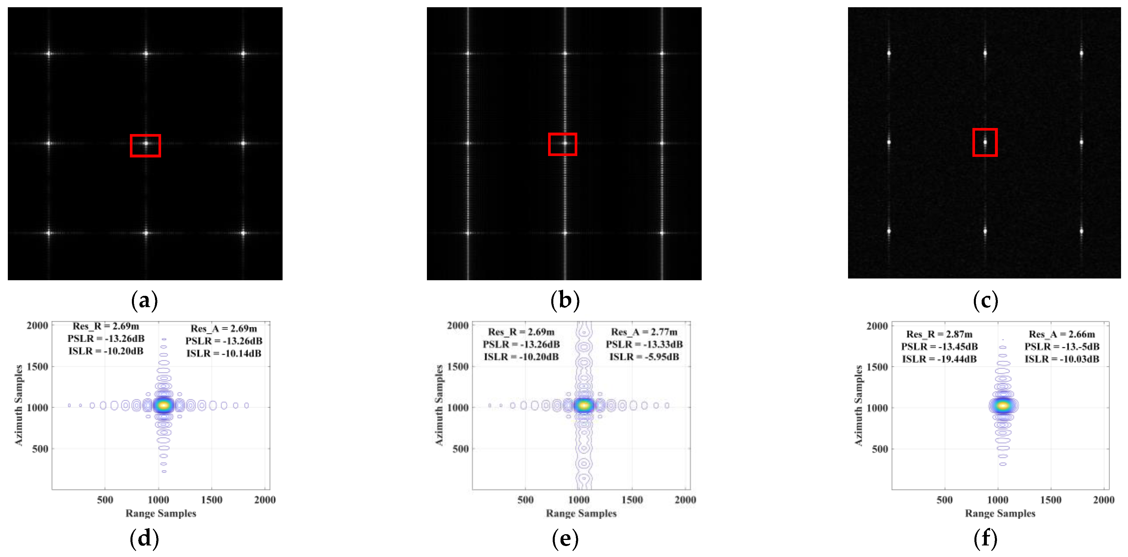
3.1. Imaging Simulations with Transmission of Chaotic FM Signals

To analyze and evaluate the performance of chaotic FM signals, one-dimensional simulation, as well as point-target and distributed-target imaging, are implemented to verify the property of resolution preservation and range ambiguity suppression in the following simulations. The corresponding simulation parameters are shown in Table 1.
(1)
Resolution Preservation
Based on the derived Formula (7), the theoretically analyzed resolution in the mainlobe is a statistically average result. In the simulation, we use 3000 one-dimensional chaotic FM signals with different initial states to calculate the resolution, and then average the result. According to the simulation parameters in Table 1, the theoretical resolution is 2.66 m, and the simulation mean resolution is 2.60 m, as illustrated in Figure 6. There exists little difference between the simulation and the theoretical analysis, which is probably due to some approximation during the theoretical deduction. Nevertheless, the resolution is approximately regarded to be preserved statistically.
(2)
Range Ambiguity Suppression
The simulations in this section demonstrate that chaotic FM signals are transmitted to avoid the mutual interferences between the current echo of near-range scatterers and the previous echo of far-range scatterers in wide-swath SAR imaging. The one-dimensional simulations in Figure 1 use the partly overlapping signal with a different delay. In the system with the transmitted LFM signals, the receiving echoes are focused when the range is compressed, but the overlapping echoes are dispersed in the final images due to the mismatching of the waveform. Compared to the chirp signals, two chaotic FM signals have a different matched filter so that only the current raw data are matched, focusing the desired targets and defocusing the unwanted. A conventional monostatic SAR system with nine-point targets is also simulated to verify this property of chaotic FM signals using the parameters shown in Table 1. In Figure 7, the simulation sets nine-point targets at the near range and the far range, respectively. Assuming that the echoes of near-range and far-range scatterers have the same echo receiving moment, the imaging result (a) in Figure 8 is the result using chirp signals without the overlapping echoes, while the results in (b) and (c) contain the echoes from the near-range and far-range scatterers, and the transmitted signals are chirp signals and chaotic FM signals, respectively. The defocusing result in (b) is due to the range-matching and azimuth-mismatching of overlapping chirp signals. The result in (c) shows focused near-range targets, and the ambiguity is not observed, which is due to the range-mismatching and azimuth-mismatching of the defocused targets. Figures (d), (e), and (f) are the contours and the corresponding evaluated index of the point targets marked with the red rectangle in (a), (b), and (c), respectively. Additionally, the quantitative analysis for the transmitted chaotic FM signals in Section 2.2.3 demonstrates that the range mainlobe and sidelobe regions of the imaging results present coherent and incoherent integration characteristics, respectively. The range sidelobes can be greatly suppressed as the number of transmitted pulses becomes large, so the range sidelobes in Figure 8f almost completely disappear. It is also demonstrated that when transmitting chaotic FM signals, the SAR system can avoid mutual interferences from echoes of near-range and far-range scatterers.

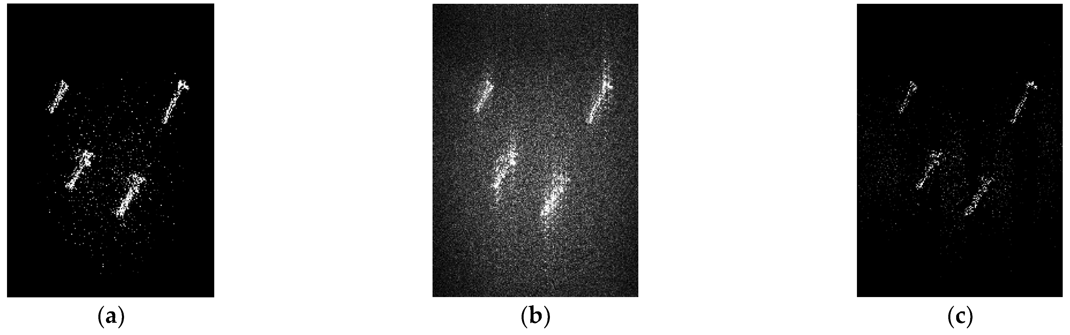
3.2. Imaging Simulations with Random PRI Variation Strategy

The PRI variation strategy decides the blind range distribution, as illustrated in Figure 2, and affects the imaging performance. In this section, the percentage of lost pulses for different PRI variation strategies is also simulated for further analysis. Figure 2 demonstrates the blind range distribution with a sequence of 500 pulses. The imaging performance is related to the accumulated pulses in the aperture time, so the percentage of lost pulses in the different slant ranges is further analyzed for different PRI variation strategies in the corresponding aperture time. As shown in Figure 9, it demonstrates that the proposed random PRI variation strategy has advantages in the uniformity of lost pulses and discontinuity of the blind range distribution compared with linear PRI variation strategies. The uniformity of lost pulses avoids a discrepancy in the imaging performance of the whole swath, and the discontinuity and irregularity of blind range can also further improve the imaging performance. Even though a slightly higher percentage of lost pulses may lead to sub-Nyquist sampling, CS theory can guarantee imaging performance. Simultaneously, random sampling is conducive to the reconstruction based on CS, which is verified by the following simulation.
The following simulations on point-target and real SAR images are used to analyze the imaging performance for different PRI strategies with the corresponding algorithms.
The elaborated PRI strategy proposed in [26,27] can achieve low missing pulses over the swath; therefore, it is chosen as the reference method combined with the BLU resampling method to compare with the proposed random PRI strategy based on the proposed algorithm in Section 2.3.
For a point target, the recovered performance can be evaluated using the resolution, PSLR, and integrated sidelobe ratio (ISLR). Point-target SAR echoes are generated using chaotic FM signals according to the parameters in Table 1. The 2D contours of point-target imaging results for different PRI variation strategies based on the corresponding imaging algorithms are demonstrated in Figure 10. For the elaborated PRI variation strategy based on the RD algorithm with the BLU method, there are false targets along the azimuth dimension, while the random PRI variation strategy based on the proposed imaging algorithm can suppress these false targets while the resolution, PSLR, and ISLR are maintained. The reason for generating false targets in the presence of an elaborated PRI variation strategy is that low-oversampling echo data may lead to sub-Nyquist sampling due to echo loss.
For a given scene σ , the recovered performance can be evaluated by relative error (RE) and structural similarity (SSIM) in this paper. RE is defined as the ratio of the error energy to the true signal energy.
RE = σ ^ σ 2 2 / σ 2 2
where σ ^ is the recovered scene. SSIM compares local patterns of pixel intensities that have been normalized for luminance and contrast [51]. In SSIM, the product of three components between the reference scene σ and the recovered scene σ ^ is computed to estimate the image local quality:
SSIM ( σ ^ , σ ) = l ( σ ^ , σ ) s 1 c ( σ ^ , σ ) s 2 s ( σ ^ , σ ) s 3
where l ( σ ^ , σ ) , c ( σ ^ , σ ) , and s ( σ ^ , σ ) are luminance comparison, contrast comparison, and structure comparison, respectively, and the calculation methods can be found in [51].
s 1 , and s 3 are positive constants used to adjust the relative importance of these three components. A simple setting s 1 = s 2 = s 3 = 1 is adopted in SSIM. Lower values of RE and larger values of SSIM represent better image quality.
In our experiments, two TerraSAR-X images, which contain urban areas and maritime targets, respectively, are used as the simulation scene. Figure 11 shows the experimental data, where (a) is a 1 m resolution image of Dubai obtained using a TerraSAR-X satellite on 12 December 2010 and (b) is a 3 m resolution TerraSAR-X image containing ship targets on the sea surface obtained on 15 April 2011.
The SAR echoes of areas in the red rectangular box in Figure 11a,b are simulated according to the parameters in Table 1 and Table 2, and the results are shown in Figure 12 and Figure 13, respectively. Figure 12a and Figure 13a are simulated using a constant PRI based on the RD algorithm for reference. Missing data will cause defocusing along the azimuth for the elaborated PRI variation strategy, which is shown in Figure 12b and Figure 13b. The recovered performance evaluated by RE and SSIM is better with the random PRI variation strategy based on the proposed imaging algorithm than the elaborated PRI variation strategy based on the RD algorithm with the BLU method, as illustrated in Table 3.

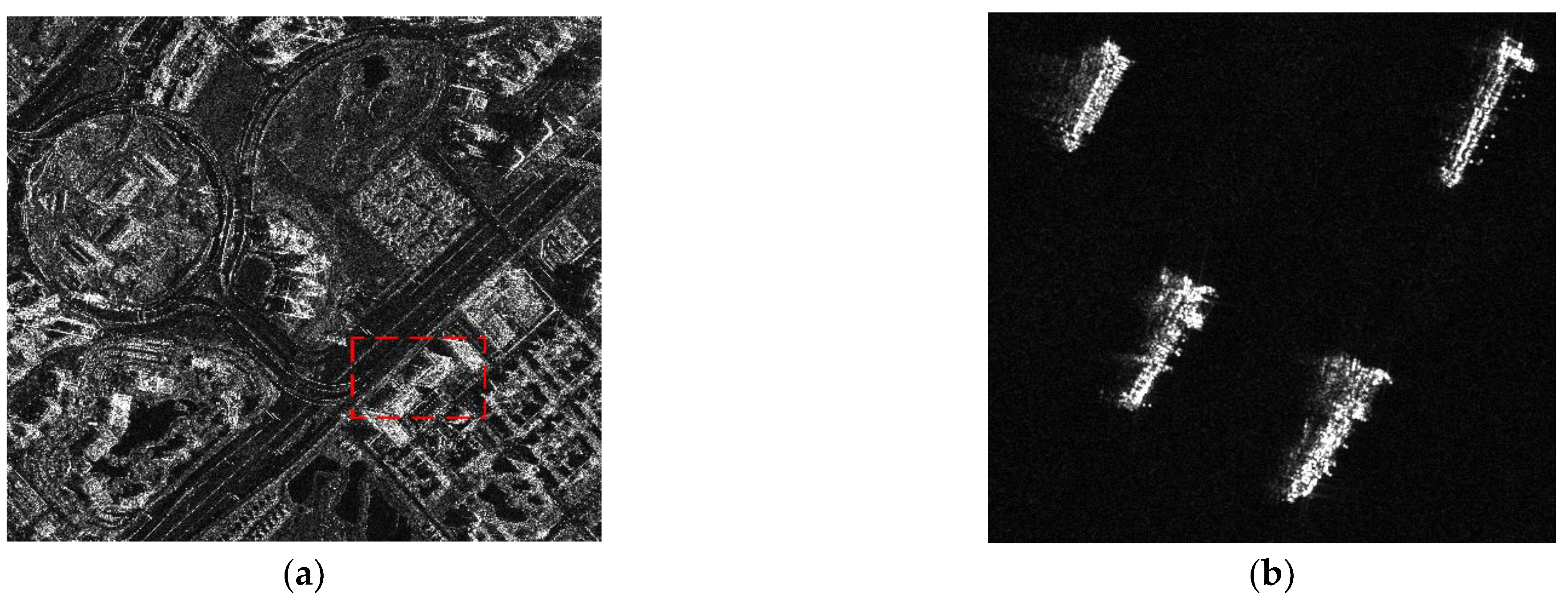
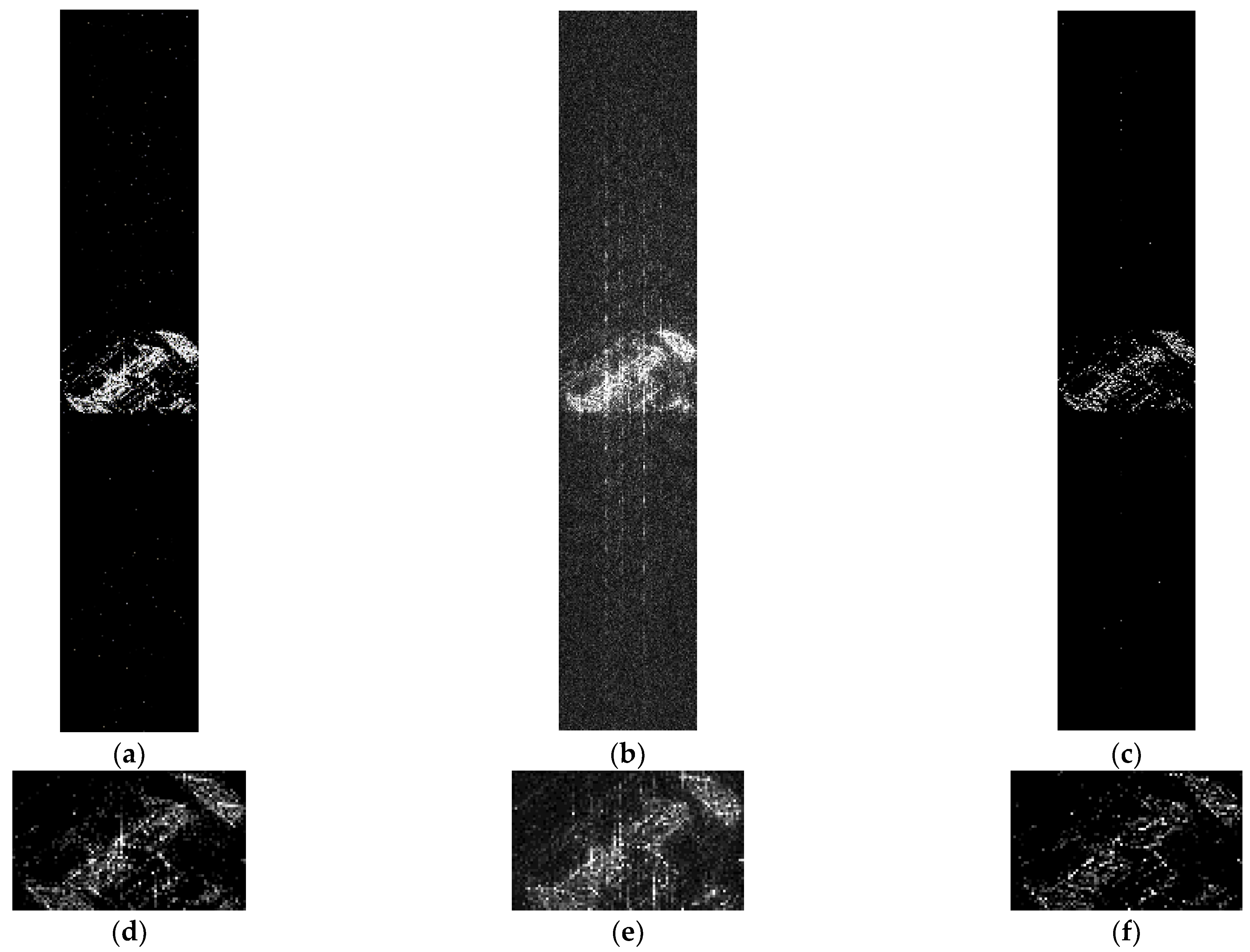
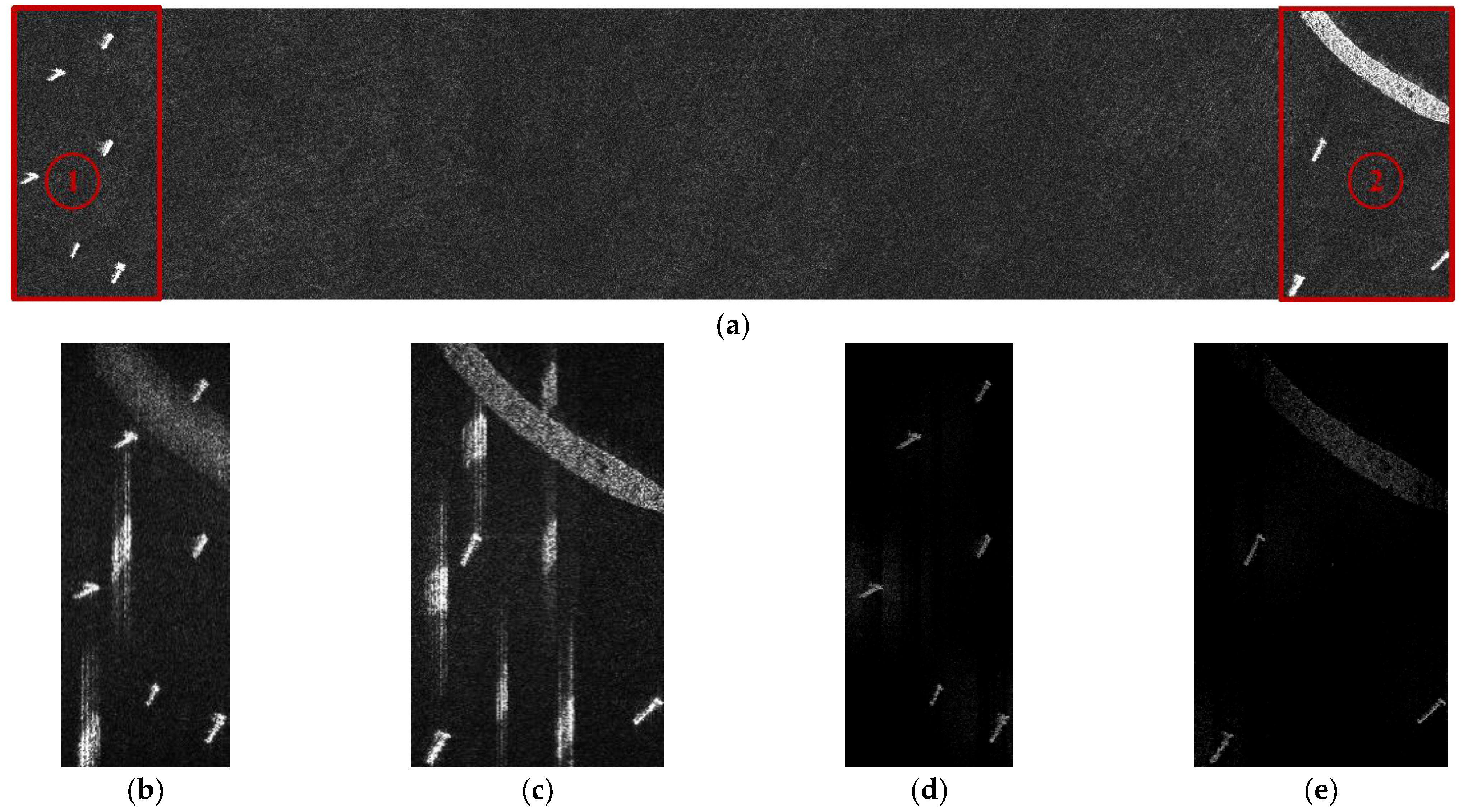
3.3. Ultra-Wide Swath Imaging System Based on Chaotic FM Signals in the Presence of a PRI Variation Strategy

To further demonstrate the effectiveness of the proposed method, a simulated experiment is carried out with a 3 m resolution TerraSAR-X image as the scene area shown in Figure 14a, assuming that Areas 1 and 2 are the near-range and far-range areas of the swath, respectively, and the raw data of Area 1 overlap with that of Area 2. Each area is reconstructed by the corresponding system parameters in Table 1. The results generated by the conventional system, namely transmitting chirp pulses with constant PRI, and the RD algorithm are illustrated in Figure 14b,c, while the results of the proposed system and imaging method are shown in Figure 14d,e. It can be seen that Figure 14b,c contains ghost targets, which are caused by the matching of the range signal and mismatching of the azimuth FM rate for the overlapping signals. The results in Figure 14d,e are close to those areas in Figure 14a and do not contain ghost targets, which demonstrates that the proposed system is capable of ultra-wide swath observation while reducing range ambiguity.

4. Discussion

This section presents the innovation of our proposed ultra-with swath SAR system by comparing it to existing technologies, which mainly include the technologies regarding DBF and SCORE, the PRI sequence optimization, and the optimal processing for low oversampling ratios, as illustrated in Figure 15.
(1)
Regarding the technologies such as DBF and SCORE
As an innovation system combined with multiple receiver apertures in elevation, staggered SAR was proposed to achieve high-resolution and wide-swath imaging in the presence of a pulse repetition interval (PRI) variation strategy [26,27]. Multiple apertures on elevation, in combination with SCan-On-REceive (SCORE), increase the system complexity and the amount of data.
In this paper, without the need for a long antenna with multiple apertures on elevation, chaotic FM signals are transmitted instead of linear frequency-modulation (LFM) signals to achieve an ultra-wide swath SAR system. The transmitted signals are time-variant so that the raw data of near-range and far-range scatters after range pulse compression avoid mutual interferences in ultra-wide imaging. Because of this, the alternative of transmitting signals enables a decrease in data volume to map an ultra-wide area without using digital beamforming (DBF).
Simultaneously, there are blind ranges due to the interruption of reception during transmission in this paper. To take full advantage of nonuniform sampling to suppress the high sidelobes due to the linear PRI variation, an optimized random PRI variation strategy is proposed to keep the PRI variation nonlinear so that the blind ranges are discontinuously and nonuniformly distributed on the whole swath.
A larger value of PRI is selected to achieve a wider swath in the proposed ultra-wide swath SAR system, which may lead to sub-Nyquist sampling. To exploit the potential of nonuniform sampling, a reconstruction algorithm based on the sparsity Bayesian learning (SBL) is proposed in the optimized random PRI variation strategy. After range compression based on the matched filtering (MF) method, range cell migration correction (RCMC) is accomplished by interpolating and summing up. During the RCMC, an innovative back-projection technique is adopted to achieve signal enhancement. Instead of resampling the nonuniform sampling signal into a uniform grid, an observation model is established and reconstructed using SBL to achieve the azimuthal compression.
(2)
Regarding the PRI sequence optimization
The blind ranges are located in
n = 1 h P R I n c 2 , n = 1 h P R I n + ι 0 c 2 , n = 2 h + 1 P R I n c 2 , n = 2 h + 1 P R I n + ι 0 c 2 , , n = l l + h 1 P R I n c 2 , n = l l + h 1 P R I n + ι 0 c 2 , R d i u s , R d i u s + H 2 R d i u s 2
where R d i u s is the radius height and H is the orbit height.
Without the limitation of the probability distribution of the random PRI sequence, many continuous pulses will be missing at some specific slant ranges. And this would bring a significant discrepancy to the imaging quality for different slant ranges in the whole swath. To avoid this discrepancy, the design principle of the PRI variation strategy should be analyzed to realize the uniformly random distribution of the blind ranges so that the blockage regions do not overlap. This means that the probability distribution of a sum of PRIs is uniformly distributed. However, it is difficult to find the sum of which probability distribution is a uniformly random distribution. In essence, the larger the variation range of PRI is, the more uniform the distribution of the blind range is. Increasing the variation range of PRI can avoid the discrepancy. In our paper, the random distribution in Formula (26) can be selected with Gaussian distribution, which has a large variation range. Compared to Reference [33], the objective function of our proposed PRI variation strategy is 0.1531 without the iteration, as demonstrated by the red point of in Figure 16. Our proposed PRI variation strategy can achieve the approximate objective function with that of Reference [33], and does not require the iteration which means it has low computation complexity.
The design of the optimum sequence in this paper is simple and does not require high oversampling to avoid the range ambiguities and data rates compared with the linear PRI variation. This nonuniform sampling method eliminates regularity and periodicity, and it avoids large gaps in the slow linear PRI variation and the tedious design in the fast linear PRI variation and the elaborated PRI variation. Additionally, compressed sensing theory guarantees that no high sidelobe is present in the azimuth impulse response after reconstruction, and the optimized random PRI variation strategy has a superior reconstruction performance under low oversampling or sub-Nyquist sampling compared to the linear PRI variation strategies. Furthermore, owing to the constraints of data volume and onboard resources, random PRI variation with a low sampling rate is of great benefit to increasing the swath width.
(3)
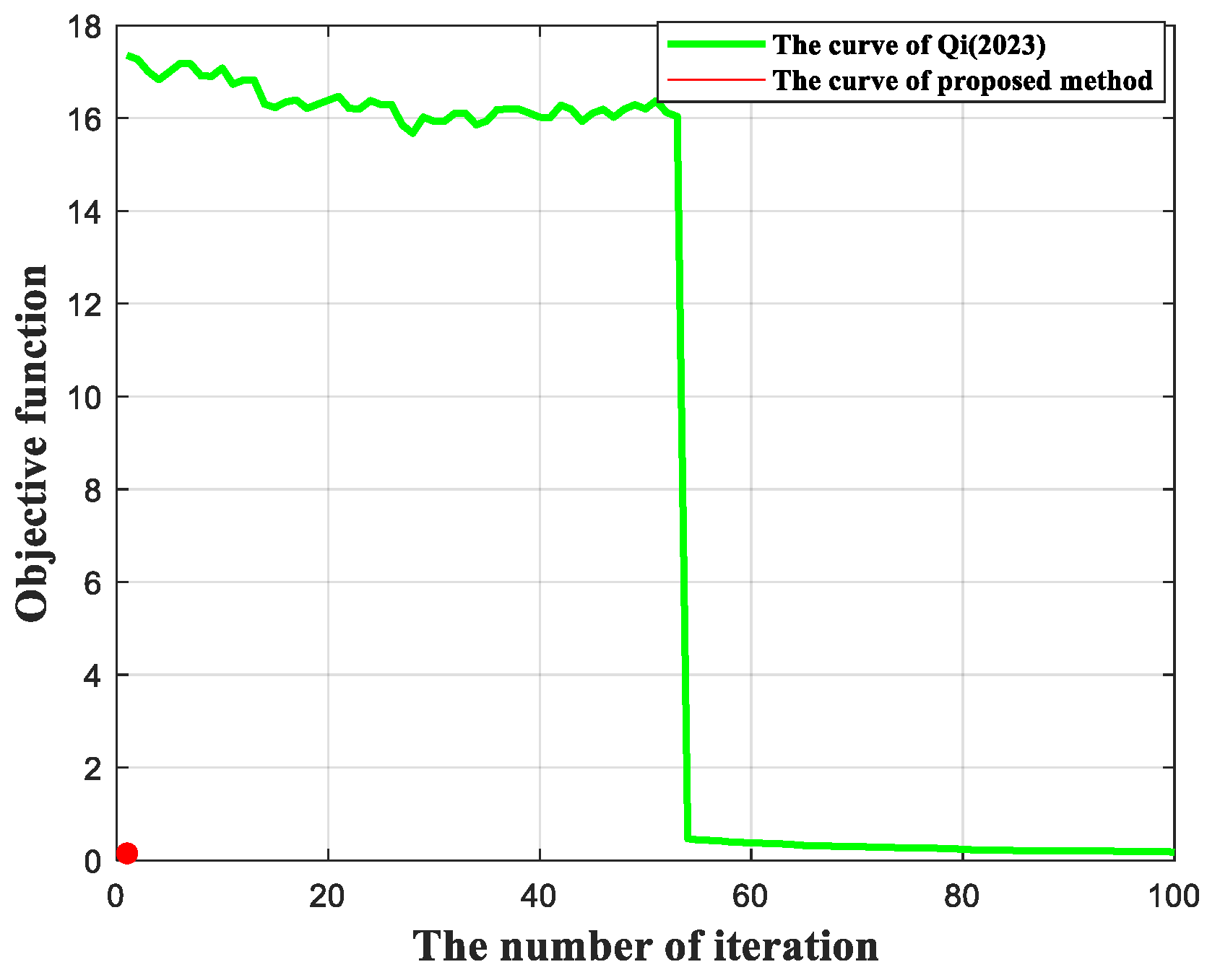
Regarding the optimal processing for low oversampling ratios
Missing data recovery methodology based on a weighted least-squares iterative adaptive approach (MIAA) in Reference [52] is a method for data recovery, and model data segments are composed of available and missing contributions. A first estimation of the spectrum is made from the available samples, and the recovery of the missing ones is obtained from this estimate and certain fitting criteria (e.g., least-squares or maximum likelihood). An updated estimation of the spectrum is performed using the now complete data segment and the data recovery/spectrum estimation procedure is possibly repeated until convergence. MIAA algorithm requires that few elements of the spectrum (if any) are equal to zero, that many elements are quite small, and that only a small number of elements have significant magnitudes. Therefore, the imaging algorithm based on MIAA in Reference [52] to recover the lost pulses provides good performance on point-like targets, while the effect on distributed targets is degraded. The SAR echoes of areas in the red rectangular box in Figure 11a are simulated according to the parameters in Table 4. As shown in Figure 17, the proposed imaging algorithm improves the performance indexes, i.e., the resolution, PSLR, and ISLR, for a point target compared to that based on MIAA in Reference [52]. For distributed scenes, there are some strips on the main target by Reference [52], which explains that the detailed information is lost. This is a common problem for most spectral estimation algorithms.
(4)
Regarding the computational cost
Consider the following:
(a)
One real multiplication and addition operation both take 1 floating point operations per second (FLOPS), and one complex multiplication and addition operation take 6 and 2 FLOPS, respectively.
(b)
The numbers of range cells and azimuth pulses are denoted by N r and N , respectively. The scene is divided into P and Q grids along range and azimuth, respectively.
(c)
One N -point fast Fourier transform (FFT) requires N / 2 log 2 N times complex multiplication and N log 2 N times complex addition, so the total computational cost is 5 N log 2 N FLOPS.
(d)
M -point complex interpolation requires M times complex multiplications and M 1 times complex additions, so the total computational cost of one single pixel point is 8 M 2 FLOPS.
For the traditional range Doppler (RD) imaging algorithm, consider the following:
Generally, the RD imaging algorithm includes range compression, RCMC, and azimuth compression. Firstly, the Fourier transform on the azimuth transforms the echo to the range-Doppler domain and requires N r times N -point FFT; the computational burden is 5 N r N log 2 N . And then each raw data takes M -point complex interpolation, and the total computational burden is N N r 8 M 2 . Finally, the imaging requires N r times N -point matched filter on the azimuth, and the total computation burden is N r 8 N 2 . Therefore, the total computational burden for the RD imaging algorithm is 5 N r N log 2 N + 2 N N r 4 M + 3 2 N r FLOPS.
For the proposed imaging algorithm, the proposed imaging algorithm includes back-projection (BP) parameter extraction, clutter suppression, and Bayesian compressive sensing (BCS) reconstruction.
a.
Parameter extraction
For each point in the scene, it requires us to calculate the position in the echo data according to the slant range and then perform M -point complex interpolation. A single point requires 8 M 1 FLOPS. Therefore, the total computational burden is P Q 8 M 1 FLOPS.
b.
Clutter suppression
It requires us to construct a N × 1 size of A m matrix and then multiply it by the extracted echo data Y e x t r a c t m to achieve A m A m H Y e x t r a c t m ; the computational load for a single range cell is 6 N + 2 N + 6 N = 14 N . Therefore, the computational load for all the points in the scene is 14 N P Q .
c.
BCS Reconstruction
The azimuth reconstruction adopts the BCS method. BCS converts the N -point complex signals into the 2 N -point real signals to further process them. The core of the BCS method is the calculation of the covariance matrix. The computational cost of the N × N covariance matrix is ο N 3 . The real iteration of the reconstruction is related to the properties of the observed scene itself; it is simplified to estimate that the computational cost for 2 N -point real signals is 8 N 3 .
In conclusion, the computational cost for the proposed imaging algorithm is P Q 8 M 1 + 8 N 3 + 14 N P Q FLOPS.

5. Conclusions

An ultra-wide swath SAR system is proposed in this paper. To avoid range ambiguity, chaotic FM signals with uniform PDFs are transmitted to replace the traditional chirp signals. Additionally, a random PRI variation strategy is adopted to make the blind ranges discontinuously and nonuniformly distributed on the whole swath. For this new system, an imaging method is also proposed, which uses time domain back-projection to correct the range cell migration and SBL to reconstruct the scene along azimuth. In future work, we will explore the on-orbit experiment to further verify the effectiveness of the proposed ultra-wide swath SAR system, and the proposed imaging method will be extended to the imaging of other high-resolution wide-swath systems.

Author Contributions

Methodology, W.C., J.G. and L.Z.; Validation, W.C. and J.G.; Writing—original draft, W.C.; Writing—review and editing, Y.G. All authors have read and agreed to the published version of the manuscript.

Funding

This research received no external funding.

Data Availability Statement

The original contributions presented in this study are included in the article. Further inquiries can be directed to the corresponding author(s).

Acknowledgments

The authors would like to thank the editors and the reviewers for their help and suggestions.

Conflicts of Interest

The authors declare no conflicts of interest.

Appendix A

In this appendix, we unfold the autocorrelation function. Assuming a chaotic FM signal can be expressed as
s 0 t = k = 1 M g τ 0 t k τ 0 + τ 0 exp j 2 π K i = 0 k 1 c i τ 0 + c k t k τ 0 + τ 0
the autocorrelation function is denoted by
R τ = + s 0 t s 0 t τ d t = M τ 0 exp j 2 π K c k τ , τ < τ 0 k = m M τ 0 exp j 2 π K c τ m τ 0 + i = k m + 1 k c i τ 0 , m 1 τ 0 < τ < m τ 0 , m 2
where τ is the time delay and M and τ 0 are the subpulse number and the subpulsewidth, respectively. K is frequency modulated rate of the chaotic FM signal. c s q c 0 = c i , i = 0 , 1 , , M 1 is the chaotic sequence and c 0 is the initial state. g τ 0 t is the unit pulse of duration τ 0 . The deduction is as follows:
When τ < τ 0 ,
R τ = k = 2 M exp j 2 π K c k 1 τ exp j 2 π K c k τ j 2 π K c k 1 c k + ( τ 0 τ ) k = 1 M exp j 2 π K c k τ M 1 exp j 2 π K c k 1 τ exp j 2 π K c k τ j 2 π K c k 1 c k + M ( τ 0 τ ) exp j 2 π K c k τ M 1 exp j 2 π K c k τ j 2 π K c k + M ( τ 0 τ ) exp j 2 π K c k τ M 1 τ exp j 2 π K c k τ + M ( τ 0 τ ) exp j 2 π K c k τ M τ 0 exp j 2 π K c k τ
When m 1 τ 0 < τ < m τ 0 , m 2 , and assuming
Q 1 τ = exp j 2 π K c k τ m 1 τ 0 exp j 2 π K c k m τ m 1 τ 0 exp j 2 π K i = k m + 1 k 1 c i τ 0 / j 2 π K c k c k m
Q 2 τ = exp j 2 π K c k m + 1 τ m τ 0 exp j 2 π K c k τ m τ 0 exp j 2 π K i = k m + 1 k c i τ 0 / j 2 π K c k c k m + 1
R τ = k = m + 1 M Q 1 τ + k = m M Q 2 τ
Q 1 τ exp j 2 π K τ m 1 τ 0 c k j 2 π K c k exp j 2 π K i = k m + 1 k 1 c i τ 0 τ m 1 τ 0 exp j 2 π K τ m τ 0 c k exp j 2 π K i = k m + 1 k c i τ 0
Q 2 τ exp j 2 π K τ m τ 0 c k j 2 π K c k exp j 2 π K i = k m + 1 k c i τ 0 m τ 0 τ exp j 2 π K τ m τ 0 c k exp j 2 π K i = k m + 1 k c i τ 0
R τ = k = m + 1 M Q 1 τ + k = m M Q 2 τ k = m + 1 M τ m 1 τ 0 exp j 2 π K τ m τ 0 c k + i = k m + 1 k c i τ 0 + k = m M m τ 0 τ exp j 2 π K τ m τ 0 c k + i = k m + 1 k c i τ 0 k = m + 1 M τ 0 exp j 2 π K τ m τ 0 c k + i = k m + 1 k c i τ 0 + m τ 0 τ exp j 2 π K τ m τ 0 c k + i = k m + 1 k c i τ 0 k = m M τ 0 exp j 2 π K τ m τ 0 c k exp j 2 π K i = k m + 1 k c i τ 0

Appendix B

In this appendix, we unfold the cross-correlation function R c τ denoted by
R c τ = + s 0 t s 1 t τ d t = M 1 τ 0 exp j 2 π K c k τ exp j 2 π K i = 0 k 1 c i 0 τ 0 i = 0 k 1 c i 1 τ 0 , τ < τ 0 k = m M τ 0 exp j 2 π K τ m τ 0 c k exp j 2 π K i = 0 k c i 0 i = 0 k m c i 1 τ 0 , m 1 τ 0 < τ < m τ 0 , m 2
The deduction is as follows:
R c τ M 1 exp j 2 π K c k τ j 2 π K c k exp j 2 π K i = 0 k 1 c i 0 τ 0 i = 0 k 1 c i 1 τ 0 M 1 exp j 2 π K c k τ τ 0 j 2 π K c k exp j 2 π K i = 0 k c i 0 τ 0 i = 0 k 1 c i 1 τ 0 M 1 τ 0 exp j 2 π K c k τ exp j 2 π K i = 0 k 1 c i 0 τ 0 i = 0 k 1 c i 1 τ 0
When m 1 τ 0 < τ < m τ 0 , m 2 , and assuming
Q 1 τ = exp j 2 π K c k 0 τ m 1 τ 0 exp j 2 π K c k m 1 τ m 1 τ 0 exp j 2 π K i = 0 k 1 c i 0 i = 0 k m c i 1 τ 0 j 2 π K c k 0 c k m 1
Q 2 τ = exp j 2 π K c k m + 1 1 τ m τ 0 exp j 2 π K c k 0 τ m τ 0 exp j 2 π K i = 0 k c i 0 i = 0 k m c i 1 τ 0 j 2 π K c k 0 c k m + 1 1
R τ = k = m + 1 M Q 1 τ + k = m M Q 2 τ
Q 2 τ = exp j 2 π K c k m + 1 1 τ m τ 0 exp j 2 π K c k 0 τ m τ 0 exp j 2 π K i = 0 k c i 0 i = 0 k m c i 1 τ 0 j 2 π K c k 0 c k m + 1 1 1 j 2 π K exp j 2 π K τ m τ 0 c k c k exp j 2 π K i = 0 k c i 0 i = 0 k m c i 1 τ 0 m τ 0 τ exp j 2 π K τ m τ 0 c k exp j 2 π K i = 0 k c i 0 i = 0 k m c i 1 τ 0
Q 1 τ = exp j 2 π K c k 0 τ m 1 τ 0 exp j 2 π K c k m 1 τ m 1 τ 0 j 2 π K c k 0 c k m 1 exp j 2 π K i = 0 k 1 c i 0 i = 0 k m c i 1 τ 0 exp j 2 π K τ m 1 τ 0 c k j 2 π K c k exp j 2 π K i = 0 k 1 c i 0 i = 0 k m c i 1 τ 0 τ m 1 τ 0 exp j 2 π K τ m τ 0 c k exp j 2 π K i = 0 k c i 0 i = 0 k m c i 1 τ 0
So,
Figure A1. Observation diagram. The red line is a curve which is on the circle with the radar as the center, Ri the radius in the imaging area, and σ 2 i , σ 3 i , , σ t i , is a series of the radar backscattering coefficients on this red line.
Remotesensing 17 01719 g0a1
R τ = k = m + 1 M Q 1 τ + k = m M Q 2 τ k = m + 1 M τ m 1 τ 0 exp j 2 π K τ m τ 0 c k exp j 2 π K i = 0 k c i 0 i = 0 k m c i 1 τ 0 + k = m M m τ 0 τ exp j 2 π K τ m τ 0 c k exp j 2 π K i = 0 k c i 0 i = 0 k m c i 1 τ 0 k = m + 1 M τ 0 exp j 2 π K τ m τ 0 c k exp j 2 π K i = 0 k c i 0 i = 0 k m c i 1 τ 0 + τ 0 exp j 2 π K τ m τ 0 c k exp j 2 π K i = 0 m c i 0 c 0 1 τ 0 k = m M τ 0 exp j 2 π K τ m τ 0 c k exp j 2 π K i = 0 k c i 0 i = 0 k m c i 1 τ 0

Appendix C

In this appendix, we derive the raw data after the projection. During this RCMC procedure, there are some clutter interferences of σ 2 i , σ 3 i , , σ t i , with the same slant range to the real target σ 1 . For a single-point target σ 1 , the raw data are denoted as
Y e x t r a c t = σ 1 exp j 4 π R 1 λ + t σ t 1 exp j 4 π R 1 λ + n 1 σ 1 exp j 4 π R 2 λ + t σ t 2 exp j 4 π R 2 λ + n 2 σ 1 exp j 4 π R N λ + t σ t N exp j 4 π R N λ + n N N × 1
where σ 2 i , σ 3 i , , σ t i , is a series of the radar backscattering coefficients on the circle with the radar as the center and R i as the radius in the imaging area, as illustrated in Figure C-1. t σ t i exp j 4 π R i / λ are essentially the clutter interferences to the signal σ 1 exp j 4 π R i / λ . To suppress these interferences, we adopt the projection method to enhance the signal. The projection vector A c u r r e n t can be denoted by
A c u r r e n t = exp j 4 π R 1 λ exp j 4 π R 2 λ exp j 4 π R N λ N × 1
The projection method makes the raw data Y e x t r a c t with the clutter interferences project on the space, which is determined by the projection vector A c u r r e n t and can be expressed by
Y b a c k = A c u r r e n t A c u r r e n t H Y e x t r a c t
After the projection, the raw data Y b a c k are
Y b a c k = A c u r r e n t A c u r r e n t H Y e x t r a c t = N σ 1 exp j 4 π R 1 λ + n 1 N σ 1 exp j 4 π R 2 λ + n 2 N σ 1 exp j 4 π R N λ + n N
n i = k = 1 N n k exp j 4 π R k λ + i = 1 N t σ t i exp j 4 π R i λ = k = 1 N n k exp j 4 π R k R i λ + i = 1 N t σ t i exp j 4 π R i λ
where n i is the superposition of multiple random complex vectors and is the incoherent accumulation. So, the accumulation is not totally proportional to the number of superpositions. After the projection A c u r r e n t , the signal is the coherent accumulation and σ 1 exp j 4 π R i / λ becomes N σ 1 exp j 4 π R i / λ . Therefore, the signal is enhanced and the clutter interferences are suppressed.

References

  1. Cumming, I.; Wong, F. Digital Signal Processing of Synthetic Aperture Radar Data: Algorithms and Implementation; Artech House: Norwood, MA, USA, 2004. [Google Scholar]
  2. Dong, B.; Li, G.; Zhang, Q. High-resolution and wide-swath imaging of spaceborne SAR via random PRF variation constrained by the coverage diagram. IEEE Trans. Geosci. Remote Sens. 2022, 60, 5241016. [Google Scholar] [CrossRef]
  3. Yang, X.; Li, G.; Sun, J.; Liu, Y.; Xia, X. High-resolution and wide-swath imaging via Poisson disk sampling and iterative shrinkage thresholding. IEEE Trans. Geosci. Remote Sens. 2019, 57, 4692–4704. [Google Scholar] [CrossRef]
  4. Guo, H.; Wang, Z.; Li, Z.; Zhang, Q.; Liu, L.; Tang, F. Wide-swath ocean current measurement based on MIMO along-track interferometry SAR. IEEE Trans. Geosci. Remote Sens. 2024, 62, 5221216. [Google Scholar] [CrossRef]
  5. Trumpf, S.; Prats-Iraola, P.; Moreira, A. Along-track deformation retrieval performance with the ROSE-L multi-channel SAR system using two-look ScanSAR. IEEE Trans. Geosci. Remote Sens. 2025, 63, 5208815. [Google Scholar] [CrossRef]
  6. Zhang, K.; Zhang, B.; Perrie, W.; Zheng, G.; Yang, J.; Fang, H. Assessment of thermal noise effect on wind speed retrieval accuracy using Sentinel-1 cross-polarized TOPSAR images. IEEE Trans. Geosci. Remote Sens. 2023, 61, 4208011. [Google Scholar] [CrossRef]
  7. Castillo, J.P.N.; Scheiber, R.; Jäger, M.; Moreira, A. Subaperture motion-adaptive reconstruction techniques for digital beamforming airborne SAR. IEEE Trans. Geosci. Remote Sens. 2024, 62, 5229518. [Google Scholar]
  8. Li, B.; Zhao, Q.; Zhang, Y.; Liang, Y.; Wang, W.; Cai, Y. An advanced sparse multichannel system for spaceborne DBF-SAR. IEEE Trans. Geosci. Remote Sens. 2023, 61, 5211513. [Google Scholar] [CrossRef]
  9. Wang, R.; Deng, Y.; Wang, W.; Zhao, Q.; Zhang, Y.; Chen, Z. A novel adaptive digital beamforming method based on beam-space phase-center cross correlation. IEEE Trans. Geosci. Remote Sens. 2023, 61, 5212213. [Google Scholar] [CrossRef]
  10. Gerhard, K. MIMO-SAR: Opportunities and pitfalls. IEEE Trans. Geosci. Remote Sens. 2013, 52, 2628–2645. [Google Scholar]
  11. Zhang, M.; Liao, G.; Xu, J.; Lan, L.; Zhu, S.; Xing, M. High-resolution and wide-swath imaging based on multifrequency pulse diversity and DPCA technique. IEEE Geosci. Remote Sens. Lett. 2021, 19, 4502505. [Google Scholar] [CrossRef]
  12. Zhang, M.; Liao, G.; Xu, J.; He, X.; Liu, Q.; Lan, L.; Li, S. High-resolution and wide-swath SAR imaging with sub-band frequency diverse array. IEEE Trans. Aerosp. Electron. Syst. 2023, 59, 172–183. [Google Scholar] [CrossRef]
  13. Wang, J.; Chen, L.; Liang, X.; Li, K. Implementation of the OFDM chirp waveform on MIMO SAR systems. IEEE Trans. Geosci. Remote Sens. 2015, 53, 5218–5228. [Google Scholar] [CrossRef]
  14. Blunt, S.D.; Mokole, E.L. Overview of radar waveform diversity. IEEE Aerosp. Electron. Syst. Mag. 2016, 31, 2–42. [Google Scholar] [CrossRef]
  15. Vespe, M.; Jones, G.; Baker, C. Lessons for radar: Waveform diversity in echolocating mammals. IEEE Signal Process. Mag. 2009, 26, 65–75. [Google Scholar] [CrossRef]
  16. Xu, W.; Huang, P.; Tan, W. Azimuth phase coding by up and down chirp modulation for range ambiguity suppression. IEEE Access. 2019, 7, 143780–143791. [Google Scholar] [CrossRef]
  17. Mittermayer, J.; Martinez, J.M. Analysis of range ambiguity suppression in SAR by up and down chirp modulation for point and distributed targets. In Proceedings of the 2003 IEEE International Geoscience and Remote Sensing Symposium (IGARSS), Toulouse, France, 21–25 July 2003. [Google Scholar]
  18. Wang, W. MIMO SAR Chirp Modulation Diversity Waveform Design. IEEE Geosci. Remote Sens. Lett. 2014, 11, 1644–1648. [Google Scholar] [CrossRef]
  19. Gao, C.; The, K.C.; Liu, A. Piecewise nonlinear frequency modulation waveform for MIMO radar. IEEE J. Sel. Topics Signal Process. 2017, 11, 379–390. [Google Scholar] [CrossRef]
  20. Jin, G.; Aubry, A.; De Maio, A.; Wang, R.; Wang, W. Quasi-orthogonal waveforms for ambiguity suppression in spaceborne quadpol SAR. IEEE Trans. Geosci. Remote Sens. 2022, 60, 5204617. [Google Scholar] [CrossRef]
  21. Hague, D.A. Adaptive transmit waveform design using multitone sinusoidal frequency modulation. IEEE Trans. Aerosp. Electron. Syst. 2021, 57, 1274–1287. [Google Scholar] [CrossRef]
  22. Xie, Q.; Yang, J.; Liu, C.; Li, W. Low sidelobe quasi-orthogonal NLFM waveforms with reciprocating frequency modulation. IEEE Geosci. Remote Sens. Lett. 2022, 19, 4027805. [Google Scholar] [CrossRef]
  23. Pappu, C.S.; Flores, B.C.; Debroux, P.; Boehm, J. An electronic implementation of Lorenz chaotic oscillator for bistatic radar applications. IEEE Trans. Aerosp. Electron. Syst. 2017, 53, 2001–2013. [Google Scholar] [CrossRef]
  24. Willsey, M.S.; Cuomo, K.V.; Oppenheim, A.V. Quasi-orthogonal wideband radar waveforms based on chaotic systems. IEEE Trans. Aerosp. Electron. Syst. 2010, 47, 1974–1984. [Google Scholar] [CrossRef]
  25. Pappu, C.S.; Flores, B.C.; Debroux, P.S.; Verdin, B.; Boehm, J. Synchronization of bistatic radar using chaotic AM and chaos-based FM waveforms. IET Radar Sonar Navigat. 2016, 11, 90–97. [Google Scholar] [CrossRef]
  26. Villano, M.; Krieger, G.; Moreira, G. Staggered SAR: High-resolution wide-swath imaging by continuous PRI variation. IEEE Trans. Geosci. Remote Sens. 2014, 52, 4462–4479. [Google Scholar] [CrossRef]
  27. Villano, M.; Krieger, G.; Moreira, A. Staggered SAR: Performance Analysis and Experiments With Real Data. IEEE Trans. Geosci. Remote Sens. 2017, 55, 6617–6638. [Google Scholar] [CrossRef]
  28. Villano, M.; Krieger, G.; Moreira, A. A novel processing strategy for staggered SAR. IEEE Geosci. Remote Sens. Lett. 2014, 11, 1891–1895. [Google Scholar] [CrossRef]
  29. Wang, X.; Wang, R.; Deng, Y.; Wang, W.; Li, N. SAR signal recovery and reconstruction in staggered mode with low oversampling factors. IEEE Geosci. Remote Sens. Lett. 2018, 15, 704–708. [Google Scholar] [CrossRef]
  30. Liu, Z.; Liao, X.; Wu, J. Image reconstruction for low-oversampled staggered SAR via HDM-FISTA. IEEE Trans. Geosci. Remote Sens. 2022, 60, 5204514. [Google Scholar] [CrossRef]
  31. Zhang, Y.; Qi, X.; Jiang, Y.; Li, H.; Liu, Z. Image reconstruction for low-oversampled staggered SAR based on sparsity Bayesian learning in the presence of a nonlinear PRI variation strategy. IEEE Trans. Geosci. Remote Sens. 2022, 60, 5229824. [Google Scholar] [CrossRef]
  32. Zhou, Z.; Deng, Y.; Wang, W.; Jia, X.; Wang, R. Linear Bayesian approaches for low-oversampled stepwise staggered SAR data. IEEE Trans. Geosci. Remote Sens. 2021, 60, 5206123. [Google Scholar] [CrossRef]
  33. Qi, X.; Zhang, Y.; Jiang, Y.; Giusti, E.; Martorella, M. Optimized nonlinear PRI variation strategy using knowledge-guided genetic algorithm for staggered SAR imaging. IEEE J. Sel. Topics Signal Process. 2023, 16, 2624–2643. [Google Scholar] [CrossRef]
  34. Wu, Y.; Fu, K.; Diao, W.; Yan, Z.; Wang, P.; Sun, X. Range sidelobe suppression approach for SAR images using chaotic FM signals. IEEE Trans. Geosci. Remote Sens. 2021, 60, 5219915. [Google Scholar] [CrossRef]
  35. Callegari, S.; Rovatti, R.; Setti, G. Spectral properties of chaos-based FM signals: Theory and simulation results. IEEE Trans. Circuits Syst. I Fundam. Theory Appl. 2003, 50, 3–15. [Google Scholar] [CrossRef]
  36. Soussen, C.; Gribonval, R.; Ldier, J.; Herzet, C. Joint K-Step Analysis of Orthogonal Matching Pursuit and Orthogonal Least Squares. IEEE Trans. Inf. Theory 2013, 59, 3158–3174. [Google Scholar] [CrossRef]
  37. Cerrone, C.; Cerull, R.; Golden, B. Carousel greedy: A generalized greedy algorithm with applications in optimization. Comput. Oper. Res. 2017, 85, 97–112. [Google Scholar] [CrossRef]
  38. Candes, E.; Tao, T. The Dantzig selector: Statistical estimation when p is much larger than n. Ann. Stat. 2007, 35, 2313–2351. [Google Scholar]
  39. Tibshirani, R. Regression shrinkage and selection via the Lasso. J. R. Stat. Soc. B 1996, 58, 267–288. [Google Scholar] [CrossRef]
  40. Ji, S.; Xue, Y.; Carin, L. Bayesian compressive sensing. IEEE Trans. Signal Process. 2008, 56, 2346–2356. [Google Scholar] [CrossRef]
  41. Tipping, M.E.; Faul, A.C. Fast marginal likelihood maximization for sparse Bayesian models. In Proceedings of the Ninth International Workshop on Artificial Intelligence and Statistics, Key West, FL, USA, 3–6 January 2003. [Google Scholar]
  42. Babacan, S.D.; Molina, R.; Katsaggelos, A.K. Bayesian compressive sensing using Laplace priors. IEEE Trans. Image Process. 2010, 19, 53–63. [Google Scholar] [CrossRef]
  43. George, E.I.; McCulloch, R.E. Approaches for Bayesian variable selection. Stat. Sin. 1997, 7, 339–373. [Google Scholar]
  44. George, E.I.; Foster, D.P. Calibration and empirical Bayes variable selection. Biometrika 2000, 87, 731–747. [Google Scholar] [CrossRef]
  45. Robert, C.P. The Bayesian Choice: From Decision-Theoretic Foundations to Computational Implementation, 2nd ed.; Springer: New York, NY, USA, 2001. [Google Scholar]
  46. Wipf, D.P. Sparse estimation with structured dictionaries. In Proceedings of the 25th International Conference on Neural Information Processing Systems, Granada, Spain, 12–15 December 2011. [Google Scholar]
  47. Pearson, K. The Problem of the Random Walk. Nature 1905, 72, 294. [Google Scholar] [CrossRef]
  48. Davenport, W.B. Probability and Random Processes: An Introduction for Applied Scientists and Engineers; McGraw-Hill Book Company: New York, NY, USA, 1970. [Google Scholar]
  49. Starck, J.L.; Murtagh, F.; Fadili, J. Sparse Image and Signal Processing: Wavelets and Related Geometric Multiscale Analysis; Cambridge Univ. Press: Cambridge, UK, 2015. [Google Scholar]
  50. Tipping, M.E. Sparse Bayesian learning and the relevance vector machine. J. Mach. Learn Res. 2001, 1, 211–244. [Google Scholar]
  51. Wang, Z.; Bovik, A.C.; Sheikh, H.R.; Simoncelli, E.P. Image quality assessment: From error visibility to structural similarity. IEEE Trans. Image Process. 2004, 13, 600–612. [Google Scholar] [CrossRef] [PubMed]
  52. Pinheiro, M.; Prats-Iraola, P.; Rodriguez-Cassola, M.; Villano, M. Analysis of low-oversampled staggered SAR data. IEEE J. Sel. Topics Signal Process. 2019, 13, 241–255. [Google Scholar] [CrossRef]
Figure 1. Transmitted signals after matched filtering.
Remotesensing 17 01719 g001
Figure 2. Examples of blind range distribution with different PRI variation strategies. The minimum and maximum slant ranges are Rmin = 635 km and Rmax = 1233 km. The pulse duration Tr = 10 us. The total number of pulses is 501.
Remotesensing 17 01719 g002aRemotesensing 17 01719 g002b
Figure 3. The autocorrelation function in the sidelobe region is demonstrated by a two-dimensional random walk model. Chaotic FM signals are modulated by the chaotic sequences with uniform probability density function (PDF) and various initial states. (a) The diagram of the two-dimensional random walk model. (b) Statistical distribution of the autocorrelation amplitude dovetails with the theoretical Rayleigh distribution. (c) Statistical distribution of the autocorrelation phase dovetails with the theoretical uniform distribution.
Remotesensing 17 01719 g003
Figure 4. The amplitude and phase of the autocorrelation function. These chaotic FM signals are modulated by the chaotic sequences with uniform PDF and various initial states. (a) The amplitude of autocorrelation function. (b) The phase of the autocorrelation function.
Remotesensing 17 01719 g004
Figure 5. Confirmation that mean ISLR improves by 10 l o g 10 N after superposition of multiple autocorrelation functions. One thousand chaotic FM signals with uniform maps and different initials are generated. The statistical ISLR improves by 29.81   dB , which is equal to the theoretical value 30   dB .
Remotesensing 17 01719 g005
Figure 6. This experiment adopts 3000 chaotic FM signals with different initial states to verify the property of resolution preservation. The resolution of each chaotic FM signal after the matched filter is different. Based on the principle of statistics, the mean resolution is 2.60 m.
Remotesensing 17 01719 g006
Figure 7. The simulation diagram.
Remotesensing 17 01719 g007
Figure 8. The experiments simulate the overlapping echoes of near-range scatters and far-range scatters when the transmitted signals are chirp signals and chaotic FM signals, respectively. Then, the result is reconstructed using traditional imaging algorithms, e.g., the RCM algorithm. (a) The reconstructed image of nine-point targets without the overlapping echoes. (b) The reconstructed image with transmitted chirp signals. (c) The reconstructed image with transmitted chaotic FM signals. Figures (df) are the corresponding evaluated indices of the marked point targets marked with the red rectangles, respectively.
Remotesensing 17 01719 g008
Figure 9. The percentage of lost pulses for different PRI variation strategies. (a) Constant PRI. (b) Slow PRI variation strategy. (c) Fast PRI variation strategy. (d) Elaborated PRI variation strategy. (e) Random PRI variation strategy.
Remotesensing 17 01719 g009
Figure 10. Two-dimensional contours of point-target imaging results for different PRI variation strategies based on corresponding imaging algorithms. (a) Constant PRIs based on the RD algorithm for reference. (b) Elaborated PRI variation strategy based on the RD algorithm with the BLU method. (c) Random PRI variation strategy based on the proposed imaging algorithm.
Remotesensing 17 01719 g010
Figure 11. Two SAR images are achieved using TerraSAR-X satellite radar and are observed in the urban area and maritime targets, respectively.
Remotesensing 17 01719 g011
Figure 12. Imaging results of urban area for different PRI variation strategies based on corresponding imaging algorithms. (a) Constant PRI based on the RD algorithm for reference. (b) Elaborated PRI variation strategy based on the RD algorithm with the BLU method. (c) Random PRI variation strategy based on the proposed imaging algorithm. The scenes in (a), (b), and (c) are zoomed in images of (d), (e), and (f), respectively.
Remotesensing 17 01719 g012
Figure 13. Imaging results of buildings for different PRI variation strategies based on corresponding imaging algorithms. (a) Constant PRI based on the RD algorithm for reference. (b) Elaborated PRI variation strategy based on the RD algorithm with the BLU method. (c) Random PRI variation strategy based on the proposed imaging algorithm.
Remotesensing 17 01719 g013
Figure 14. The experiments simulate the overlapping echoes of near-range scatters in Area 1 and far-range scatters in Area 2 when the transmitted signals are chirp signals and chaotic FM signals, respectively. Area 1 and Area 2 are marked by red boxes and represented by ① and ②, respectively. Then, the result is reconstructed by RDA and the proposed method, respectively. (a) Referenced image is achieved by TerraSAR-X satellite radar and observed in maritime. Figures (b) and (c) are the reconstructed area 1 and area 2 with transmitted chirp signals, respectively. Figures (d,e) are the reconstructed area 1 and area 2 with transmitted chaotic FM signals.
Remotesensing 17 01719 g014
Figure 15. The challenges of an ultra-wide swath SAR system and the corresponding solutions of the time-variant transmission of CFM signals, the random PRI variation strategy, and the reconstruction algorithm based on SBL.
Remotesensing 17 01719 g015
Figure 16. Plot of the objection function versus iteration number. Red point (1, 0.1531): the objective value of our proposed PRI variation strategy. Green dashed line: the objective value of Qi [33] as the iteration number.
Remotesensing 17 01719 g016
Figure 17. The imaging results obtained when recovering with Reference [52] and our proposed imaging algorithm. Figures (a,c) are the recovered results of a point target based on MIAA in Reference [52], and (b,d) are the recovered results of distributed scenes based on the proposed algorithm in our paper.
Remotesensing 17 01719 g017
Table 1. Simulated parameters.
ParameterChaotic FM SignalsLFM Signals
Signal Bandwidth (MHz)5050
Sampling Frequency (MHz)6060
Subpulse Width (us)1.67 × 10⁻²
Subpulse Number600
Modulated Rate (MHz/s)50
Pulse Width (us)1010
Wavelength (m)0.030.03
Chaotic Mapping NameBernoulli
Height (Km)600600
Velocity (m/s)71007100
Antenna Length (m)5.325.32
(Mean) Pulse Repetition Frequency (Hz)27753593
Doppler Bandwidth (Hz)26712671
Looking Angle in the near-range (rad)0.40.4
Looking Angle in the far-range (rad)0.80.8
Table 2. Simulated parameters.
ParameterChaotic FM SignalsLFM Signals
Signal Bandwidth (MHz)26.5826.58
Sampling Frequency (MHz)39.539.5
Modulated Rate (MHz/s)26.58
Pulse Width (us)1010
Wavelength (m)0.030.03
Chaotic Mapping NameBernoulli
Height (Km)600600
Velocity (m/s)71007100
Antenna Length (m)1010
(Mean) Pulse Repetition Frequency (Hz)14911860
Doppler Bandwidth (Hz)14201420
Table 3. Evaluated results.
RESSIM
Figure 12(b)6.06290.6887
(c)0.77700.9809
Figure 13(b)1.12580.6693
(c)0.68690.9759
Table 4. Simulated results.
ParameterValue
The Doppler Bandwidth (Hz)2367
The oversampling ratio1.06
The percentage of lost pulses10%
Antenna Length (m)6
Disclaimer/Publisher’s Note: The statements, opinions and data contained in all publications are solely those of the individual author(s) and contributor(s) and not of MDPI and/or the editor(s). MDPI and/or the editor(s) disclaim responsibility for any injury to people or property resulting from any ideas, methods, instructions or products referred to in the content.

