1. Introduction
Due to the imbalance between energy budgets on both sides of a sunny–shady slope, a considerable section of the permafrost subgrade along the QTH has formed an asymmetrical thaw plate under the action of perennial freeze–thaw cycles. This asymmetrical thaw plate contributes to various engineering faults, including longitudinal cracks and slope collapses, which have worsened in recent years [
1,
2,
3]. Therefore, research on the prediction and spatial zoning of asymmetric thaw plate characteristics under the influence of the sunny–shady slope effect (SSSE) is of great significance, which can provide critical technical references for the scientific design, quality improvement and renovation of the QTH.
Numerous studies have demonstrated the significant impact of the SSSE on permafrost temperature fields and freeze–thaw characteristics. Lan et al. [
4] found that soil temperatures at various depths on the sunny slope were significantly higher than those on the shady slope. Hu et al. [
5], through multi-section ground temperature monitoring, confirmed the significant influence of the SSSE on temperature fields in permafrost regions and its widespread occurrence. Song et al. [
6] further identified pronounced asymmetry in roadbed temperature fields with the top surface of the permafrost on the sunny slope being lower than that on the shady slope [
7]. Chou et al. [
8] demonstrated that the temperature and thaw depth on the sunny slope were significantly higher than those on the shady slope with roadbed deformation lagging behind in terms of temperature changes. Ren et al. [
9] revealed that the SSSE caused asymmetric freezing and thawing characteristics between the sunny and shady slopes due to differences in solar radiation. Chen et al. [
10] summarized the effects of the sunny–shady slope phenomenon on roadbed heat flow and thaw characteristics, emphasizing its potential to cause asymmetric damage to road structures. Tai et al. [
11] highlighted the critical roles of road orientation and the SSSE in influencing roadbed frost heave, thaw settlement, and temperature distribution, and they further proposed strategies to mitigate these effects.
Meanwhile, remote sensing technology has been widely used in permafrost research. Shi et al. [
12] mapped the permafrost distribution across the Qinghai–Tibet Plateau by integrating a decision tree algorithm with critical environmental drivers, including topography and vegetation. Khan et al. [
13] employed multi-source satellite imagery to quantify the extent of permafrost in the western Himalayas at a 30 m spatial resolution. In contrast, Oldenborger et al. [
14] applied a supervised classification approach to assess thaw sensitivity in Nunavut’s Rankin Inlet, Canada, based on geological, topographical, and multispectral variables. Wang et al. [
15] revealed the thermodynamic mechanism of thermokarst development in the Qinghai–Tibet Plateau and its coupling relationship with climate factors through the cooperative observation of optical and radar remote sensing. Shan et al. [
16] integrated the SBAS-InSAR technology and the surface frost number model, and they successfully determined the spatio-temporal differentiation of surface deformation along the Beihei Highway using multi-time series remote sensing data. For long-term trend quantification, Zhao et al. [
17] employed an earth system model, remote sensing datasets, and field observations to quantify the long-term changes in permafrost thickness on the Qinghai–Tibet Plateau from 1851 to 2100. Similarly, Gao et al. [
18] combined remote sensing, GIS techniques, and numerical simulations to systematically analyze the feedback mechanisms between vegetation succession and permafrost temperature fields in the Mohe region. Zhang et al. [
19] combined the climate-permafrost model with a machine learning scheme to invert the thickness of the active layer of Alaska based on high-resolution remote sensing data.
In summary, previous studies have revealed the significant impact of the SSSE on permafrost temperature fields and thawing processes, and they also have conducted in-depth investigations on the distribution of permafrost and its evolutionary characteristics by the use of remote sensing technology. However, quantitative analyses of the spatial distribution characteristics of the asymmetric thawing plate of the QTH caused by the SSSE remain limited. To this end, three indictors were proposed to depict the asymmetric thaw plate of the QTH in this work: road shoulder thawing depth difference (RSTDD), offset distance (OD), and active layer thickness difference (ALTD). Based on Moderate Resolution Imaging Spectrometer (MODIS) remote sensing data and large-scale geological survey data acquired by the project “Upgrading and Reconstruction of the G109 Section from Golmud to Nagqu on the QTH” [
20], an earth–atmosphere coupled numerical model and a random forest (RF) method were employed to predict the morphological characteristic of an asymmetric thaw plate of permafrost subgrade. Then, the spatial distribution characteristics of morphological indictors along the QTH and the pattern of influence of engineering geological factors on the indictors were also analyzed.
2. Materials and Methods
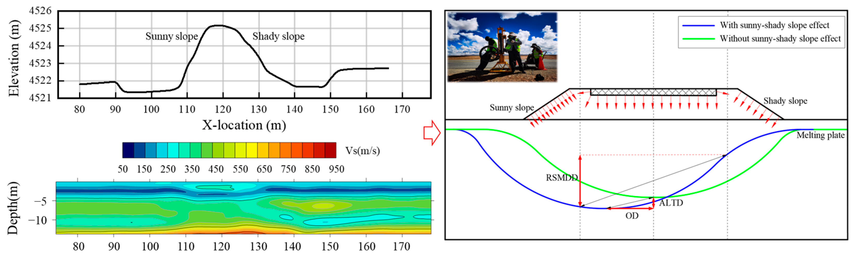
A field investigation was conducted at section K2935+050 of the QTH to examine the characteristics of the permafrost subgrade. This site is located in the Chumar River High Plain with the subgrade oriented 18° east–northeast. The surface is sparsely vegetated, and the lithology is primarily composed of silty clay, marl, mudstone, and gravelly sandstone. The ice type is a soil–ice layer, and the subgrade exhibits moderate settlement. The morphology of the thaw plate was obtained using the seismic surface wave inversion method, as shown in
Figure 1. In the testing results, the thaw plate of the permafrost subgrade under the action of a sunny–shady slope showed an obvious asymmetric distribution characteristic. The active layer thickness (ALT) was displaced greatly toward the sunny slope, and the thaw depth also exhibited a significant difference between the sunny and shady slopes. Therefore, three indictors were established in this work to evaluate the morphological patterns of the asymmetric thaw plate of the permafrost subgrade along the QTH as follows:
(1) RSTDD represents the difference in thaw depth between the sunny and shady slopes at the road shoulders. It reflects the disparity in heat transfer outcomes between the two slopes. The expression is
where
Dsun and
Dshade represent the thaw depths at the sunny and shady slopes of the road shoulders, respectively;
(2) OD indicates the extent of displacement of the ALT toward the sunny slope, reflecting the asymmetry in the thaw plate shape. The expression is
where
XALT,sun denotes the horizontal position of the ALT on the sunny slope, while
Xcenter represents the center position of the roadbed;
(3) ALTD represents the difference in ALT between uniform and sunny–shady slope conditions. The expression is
where
ALTuniform and
ALTsun-shade represent the ALT without and with sunny–shady slope conditions, respectively.
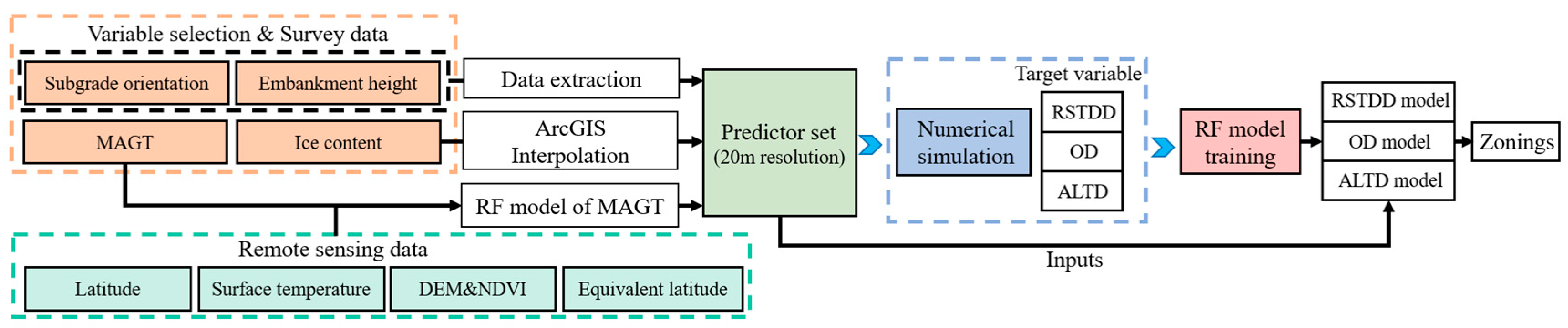
To predict the spatial distribution of morphological indicators of an asymmetric thaw plate along the QTH, an integrated evaluation framework combining data processing, numerical simulation, and an RF prediction model was developed in this work. As shown in
Figure 2, the workflow comprises the following steps: (1) correlation analysis between predictors and target parameters (RSTDD, OD, and ALTD), involving screening and combining different predictor sets to determine the final predictor set; (2) collecting, downloading, and processing the remote sensing and geological survey data, providing an inversion dataset of 4 predictors with 20 m resolution; (3) determining a reasonable numerical calculation scheme through orthogonal design, calculating the morphological indicators of the asymmetric thawing plate of the permafrost subgrade at representative locations along the QTH, and obtaining a training sample set; and (4) establishing the RF prediction model and predicting the spatial distributions of RSTDD, OD, and ALTD, respectively.
2.1. Data Resource
Remote sensing and large-scale geological survey data, covering the entire 530 km permafrost area along the QTH, were collected to aid in predicting the spatial distribution characteristic of morphological indictors. The remote sensing data included surface temperature, normalized difference vegetation index (NDVI), digital elevation model (DEM), latitude and equivalent latitude, which were derived from the MODIS dataset. The geological survey data included field monitoring data, drilling data, survey data and QTH engineering design data. A detailed description of the dataset is given in
Table 1. All datasets were subjected to downscaling and spatial resampling to ensure consistency and comparability in spatial resolution across different data sources. Ultimately, all data were uniformly processed and analyzed at a 20 m spatial resolution to support subsequent modeling and spatial analyses.
(1) Remote sensing data: The remote sensing data were downloaded from the Google Earth Engine (GEE) platform database (
https://developers.google.cn/earth-engine, accessed on 18 May 2024). Among them, the surface temperature was obtained from the MODIS land surface temperature (LST) data product (MOD11A2 V6.1 dataset), using the effective value of daily average LST. The NDVI was used to reflect the vegetation growth condition, and it was obtained from Landsat optical remote sensing data products (Landsat 5, Landsat 7 and Landsat 8 dataset). The elevation data were extracted based on the MODIS SRTM DEM-V3 data product. Slope, slope direction and latitude data were calculated in the GEE platform with MODIS SRTM DEM-V3 data using the ee.Algorithms.Terrain function and pixelLonLat function, respectively. In addition, equivalent latitude is a long-term potential factor of direct solar radiation on the surface, which is calculated as shown below [
21]:
where
k is the slope angle,
l is the aspect, and
φ refers to the latitude.
The data sources and resolutions of all six types of remote sensing data are shown in
Table 2. These data were classified and preprocessed, and then they were used as the predictor dataset of MAGT.
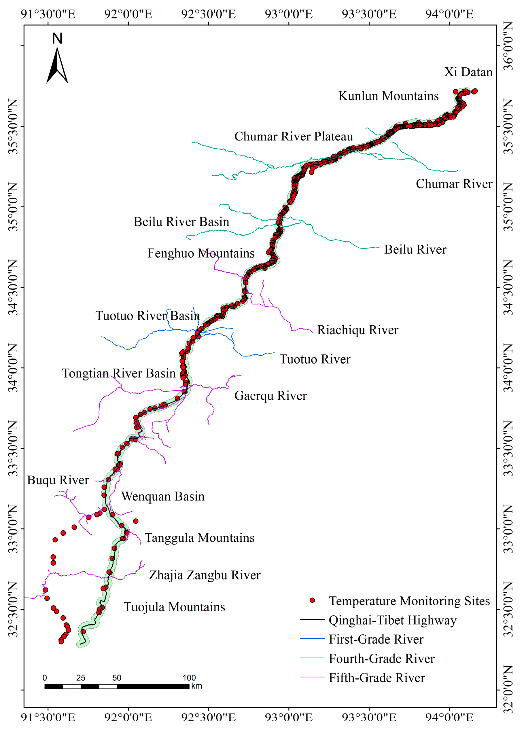
(2) Field monitoring data: Ground temperature data were derived from long-term ground temperature monitoring sections along the QTH. The data monitoring period was from 2018 to 2024, with a total of 612 ground temperature data points, whose distributions are shown in
Figure 3.
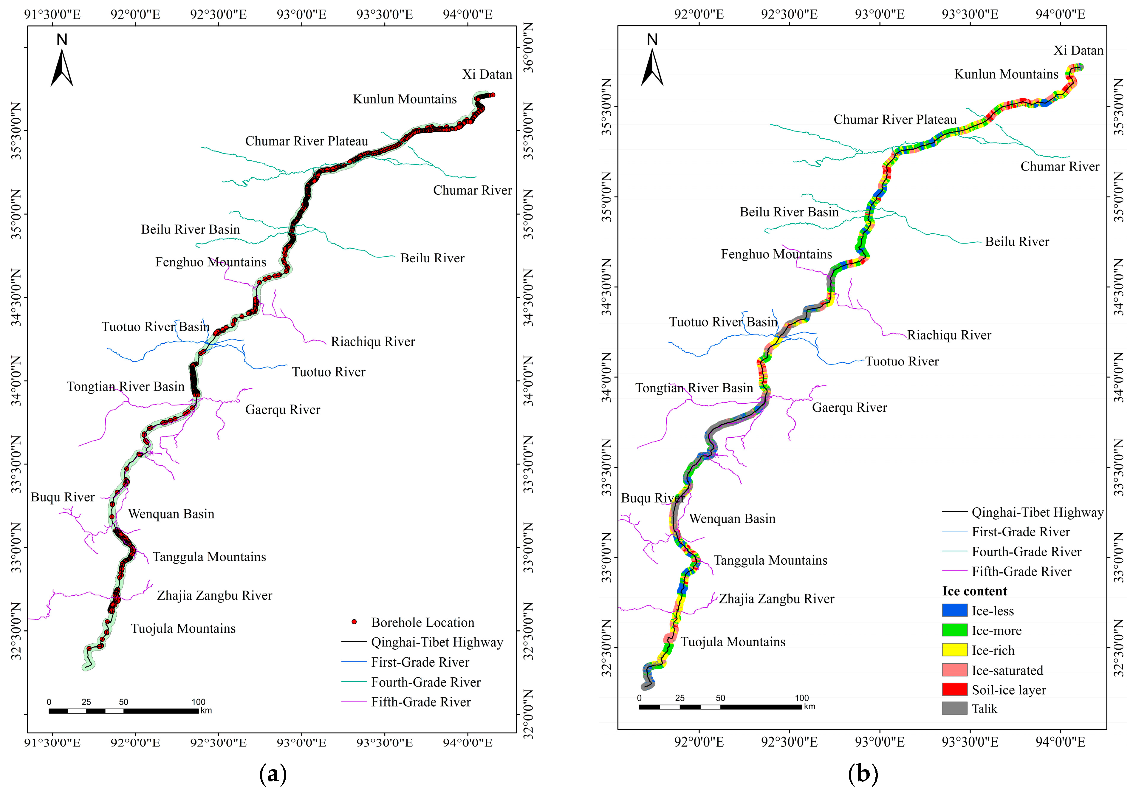
(3) Drilling data: The ice content data were determined with reference to the collected information of 2188 drilling boreholes along the QTH, which were obtained in March–October 2024. Considering that the ice content would be greatly changed under the action of long-term drastic heat transfer processes in the overlying subgrade structure, 1428 natural ground boreholes were selected from 2188 original drilling boreholes (
Figure 4a). The classification of ice content followed the guidelines in [
22], which include categories such as ice-poor, ice-rich, and ice-saturated soils based on the visual observation of segregated ice, ice films around particles, and ice layer thickness. Using the inverse distance weighting method in ArcGIS 10.8, a spatial distribution map of permafrost ice content was generated along the QTH, as shown in
Figure 4b.
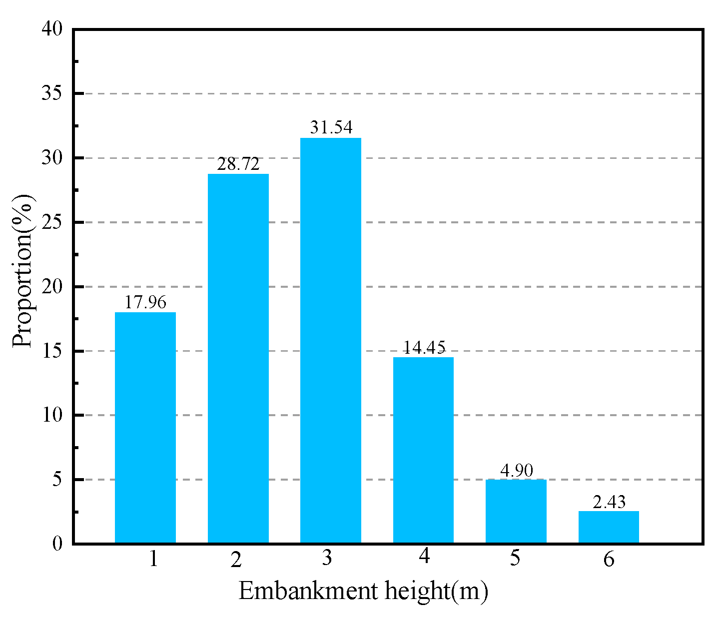
(4) Survey data and engineering design data: The embankment height data along the QTH were derived from the survey results of subgrade profile mapping work, which was conducted in 2024. Although the raw data of the subgrade cross-section were extracted at intervals of 5 m or 20 m, embankment height data were interpolated at 20 m intervals to unify the data sparsity. The probability distribution of embankment height along the QTH was calculated, as shown in
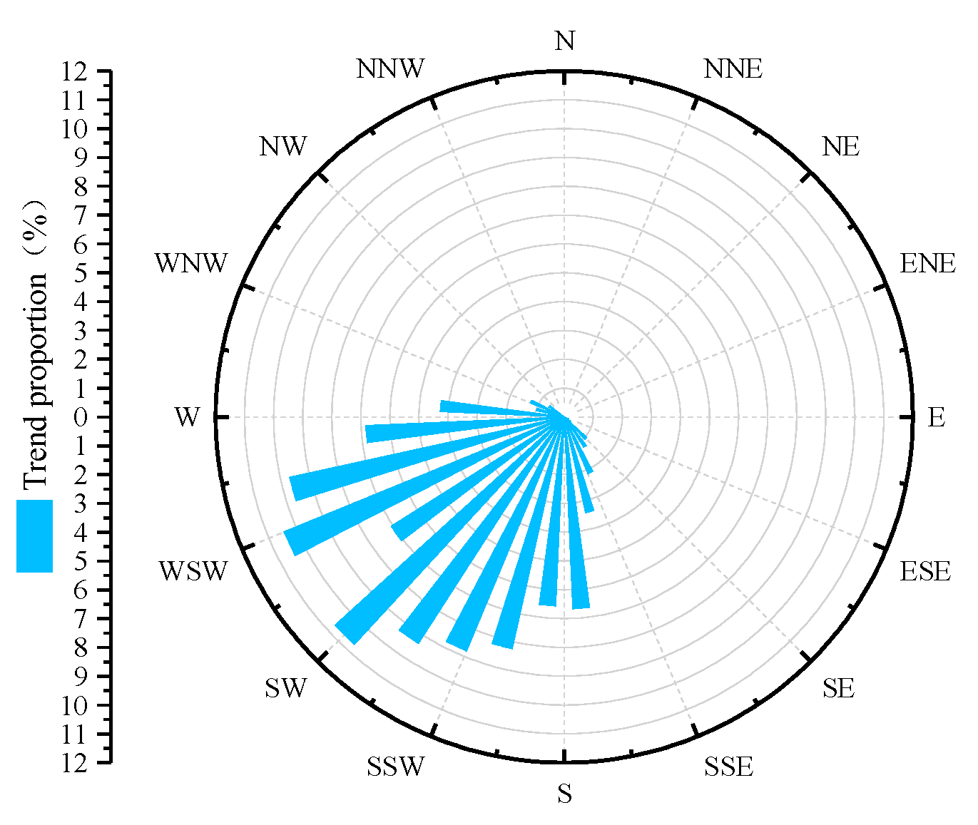
Figure 5. The most probable embankment height along the QTH is 3 m. The subgrade orientation data were calculated based on the route design scheme of the QTH. Similarly, in order to unify the data resolution, the interval of the subgrade orientation data was also processed to be 20 m. A statistical rose diagram of the subgrade orientation along the QTH was obtained, as shown in
Figure 6. It shows that west–south is the main subgrade orientation of the QTH, with WSW and SW being especially prevalent, accounting for 10.44% and 10.71%, respectively.
2.2. Numerical Approach of Asymmetric Thaw Plates’ Morphological Indicators
2.2.1. Numerical Model
The earth–atmosphere coupled numerical model [
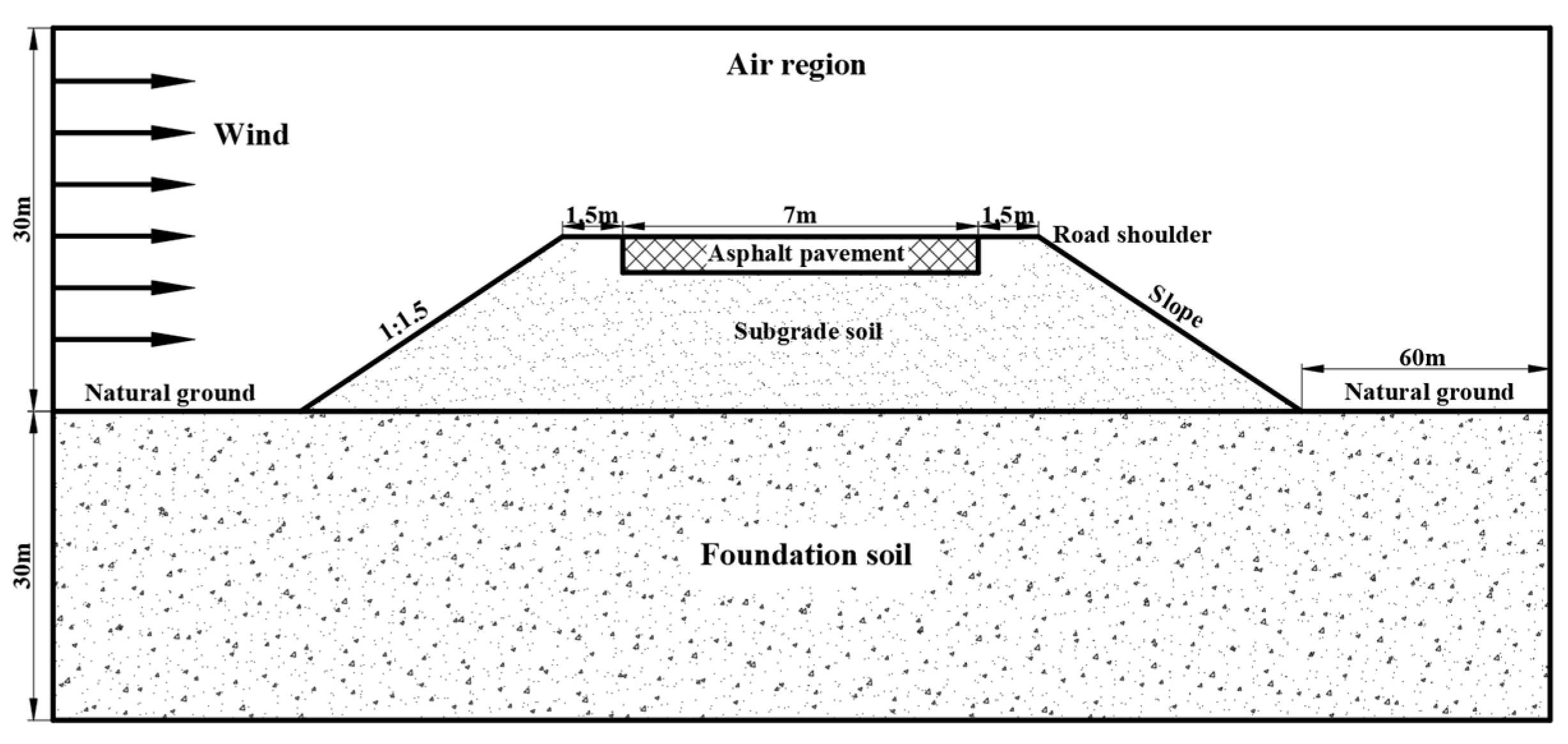
14] was employed to predict the morphological indicators of an asymmetric thaw plate of permafrost subgrade. The physical model of the permafrost subgrade was divided into four regions: the air zone, the asphalt layer, the embankment fill, and the underlying permafrost, as shown in
Figure 7. Based on the field geological survey of the QTH subgrade, the width of the embankment was 10 m with bilateral 1.5 m soil shoulders, and the thickness of the asphalt layer was 0.3 m. The height of the upper air region was defined as 30 m, and the length of the bilateral natural permafrost was set as 60 m to avoid the influence of the external environment. Meanwhile, to enhance the model’s general applicability, the natural permafrost layer was simplified to a 30 m thick single soil type. According to ice content, the permafrost layer was divided into 5 types: less-ice permafrost (
S), more-ice permafrost (
D), ice-rich permafrost (
F), ice-saturated permafrost (
B), and the soil-ice layer (
H) [
22]. The physical parameters of the permafrost layer were calculated based on the empirical formula proposed by Xu et al. [
23], using the average dry density and water content of specific soil types, as listed in
Table 3. The physical parameters of the air region, asphalt pavement, and embankment fill were determined in [
24].
2.2.2. Numerical Procedures
A 2D transient solver was adopted in the numerical calculation [
22]. The standard
-
model was employed for turbulence simulation in the air region. Given that the air environment was introduced into the computational model, the corresponding boundary conditions needed to reflect the complex earth–atmosphere coupling heat transfer process. The detailed boundary conditions settings were devised as follows.
(1) The upper boundary of the air region was set as the temperature boundary condition. Global warming was considered by applying a warming rate of 0.022 °C·year
−1 [
22,
24]. Meteorological station data from the national meteorological information center (NMIC) of China (
https://data.cma.cn, accessed on 1 June 2024) were used to fit the empirical temperature variation formula,
where
Tair is the ambient temperature;
t is the day number, with August 20 set as
t = 0;
A is the average annual air temperature; and
Tyear is the year corresponding to the calculation time.
(2) Left and right boundaries of the air region were set as the velocity inlet boundary conditions. The temperature setting was consistent with the upper boundary of the air region. A scheme program was used to dynamically adjust theind direction, and the adjustment timing was also based on local meteorological data. The wind speed (
v) was modeled as a function of height (
x) above the ground [
24],
where
vref is the wind speed at a reference height of 10 m, which is taken as the monthly average wind speed provided by the NMIC.
(3) The left and right boundaries of the permafrost region were set as adiabatic walls, while the bottom boundary was assigned a geothermal heat flux of 0.06 W·m
−2 to account for geothermal influence [
24].
(4) The surfaces of the embankment layers and natural ground were defined as coupled wall boundary conditions with a thickness of 0.1 m. The equation is
where
Qsun,
Qrad and
Qevap are the total solar radiation projected to the surface, the long-wave radiation heat loss from the surface to the environment and the evaporation heat loss from the surface moisture, respectively;
α is the surface absorption coefficient;
X is the radiative angle factor; and
k is the slope coefficient, taking account of the combined effects of direct solar radiation and diffused solar radiation, which can be calculated as [
25]
where
kd is the slope coefficient of direct solar radiation. For the sunny slope and shady slope, it can be calculated as follows [
26]:
where
αroad is the subgrade slope angle;
β is the solar elevation angle;
δ is the subgrade orientation; and
θ is the solar azimuth angle.
In order to obtain numerical results of the asymmetric thaw plate morphological indicators that are as abundant and representative as possible, the influencing factors such as subgrade orientation, embankment height, ice content and MAGT were considered in the numerical calculation scheme design. The level ranges of factors were determined based on field-measured data, except for MAGT, the range of which was defined according to the classification proposed by Cheng [
27], as shown in
Table 4. Furthermore, to reduce the number of computation cases while maximizing factor combinations, an orthogonal design strategy was adopted. Through the orthogonal design of the above influencing factors and levels, a total of 128 numerical cases were finally designed and calculated.
All numerical simulations were performed using ANSYS Fluent 2022 R1, which is a platform that has been widely adopted for earth–atmosphere coupled heat transfer modeling. The computational domain was discretized using an unstructured quadrilateral mesh, with local mesh refinement applied specifically in the vicinity of the embankment region, to accurately resolve steep thermal gradients. A second-order upwind scheme was employed for the discretization of convection–diffusion terms. Convergence was considered achieved when the residuals of the energy equations fell below 10−5 with a maximum of 200 iterations per time step imposed to ensure computational stability and numerical accuracy.
2.3. Random Forest Prediction Model of Asymmetric Thaw Plates Morphological Indicators
Considering the complex nonlinear relationships among environmental parameters along the QTH, traditional regression models struggle to capture multi-factor interactions. The RF method was selected as the core predictive tool in this study due to its high accuracy, strong noise resistance, and ability to mitigate overfitting [
28]. In this paper, the Scikit-learn machine learning library (
https://scikit-learn.org/) in Python was used as the foundational tool for model development. By employing bootstrapping, subsets were repeatedly extracted from the training dataset with replacement, and independent decision trees were trained on these subsets. Finally, the average result of the decision trees was calculated to estimate the outputs for RSTDD, OD, and ALTD. To ensure model validation, the dataset was randomly divided into training and testing sets in an 8:2 ratio. Specifically, RF regression models were developed to predict the talik, MAGT, RSTDD, OD, and ALTD.
2.3.1. RF Prediction Model of Talik Area and MAGT
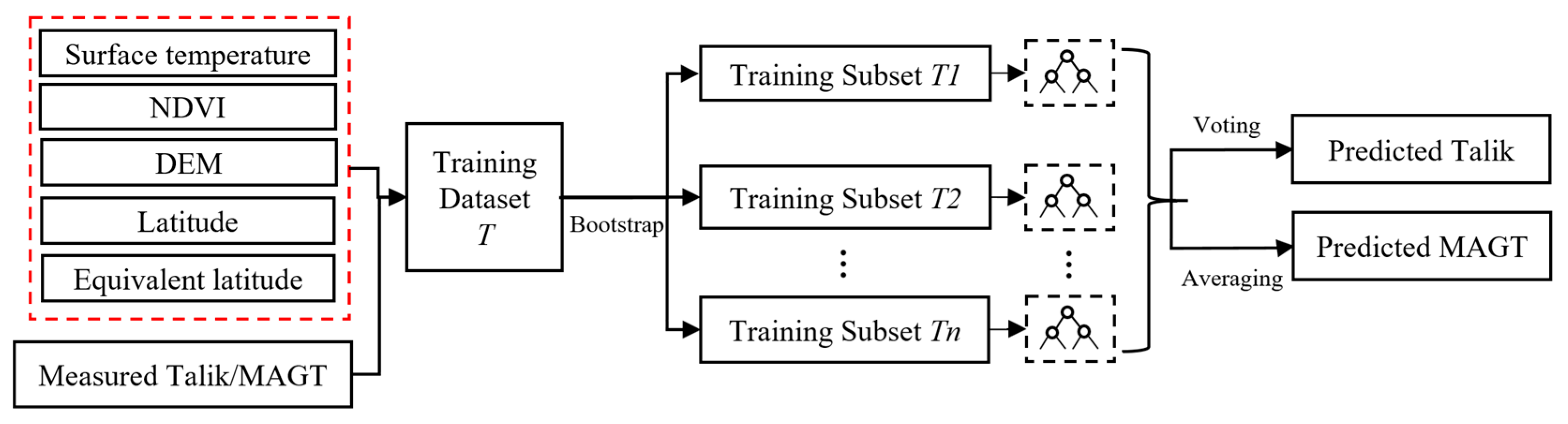
The RF regression model was employed for predicting the talik area and MAGT along the QTH. As shown in
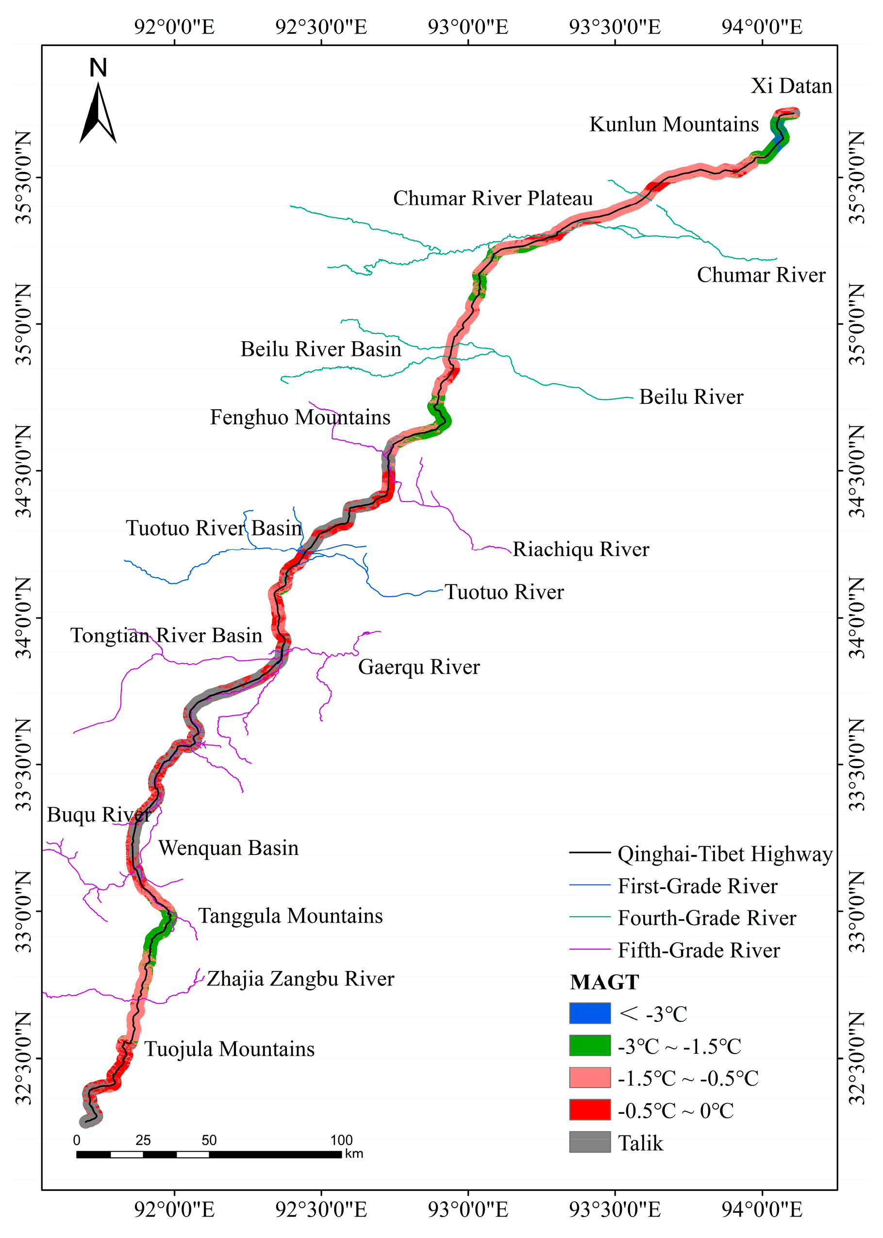
Figure 8, the surface temperature, NDVI, DEM, latitude and equivalent latitude of these 612 data points were extracted as the feature variables, and the monitoring MAGT was used as the target variable. In addition, the identification of talik area was the premise of MAGT prediction. Therefore, a similar RF model and feature variable system were adopted for the identification of the talik area in this work, and we took “whether belongs to the Talik” as the binary classification target variable. Integrating 2800 data points (including 2188 items of drilling borehole data and 612 items of ground temperature monitoring data), the zoning map of the talik area and MAGT within 5 km along the QTH were predicted (
Figure 9).
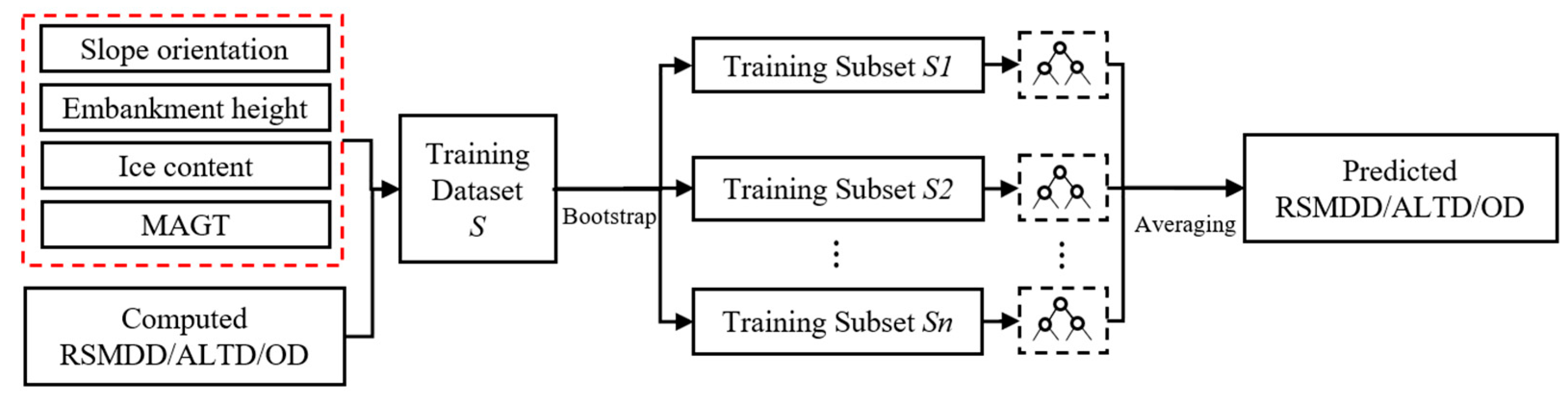
2.3.2. RF Prediction Model of RSTDD, OD and ALTD
In order to determine the predictor sets of RSTDD, OD and ALTD, we systematically analyzed the influencing factors that determine the morphology of the permafrost subgrade’s thaw plate [
2,
6,
29,
30,
31]. Screening and correlation analyses between the influencing factors and target parameters were conducted, and the prediction effects of different combinations of predictor sets were compared. Finally, four factors were selected for evaluating the asymmetric thaw plates: subgrade orientation (angle relative to the east–west direction), embankment height, ice content, and MAGT. The scheme diagram of the RF model for RSTDD, OD and ALTD is given in
Figure 10.
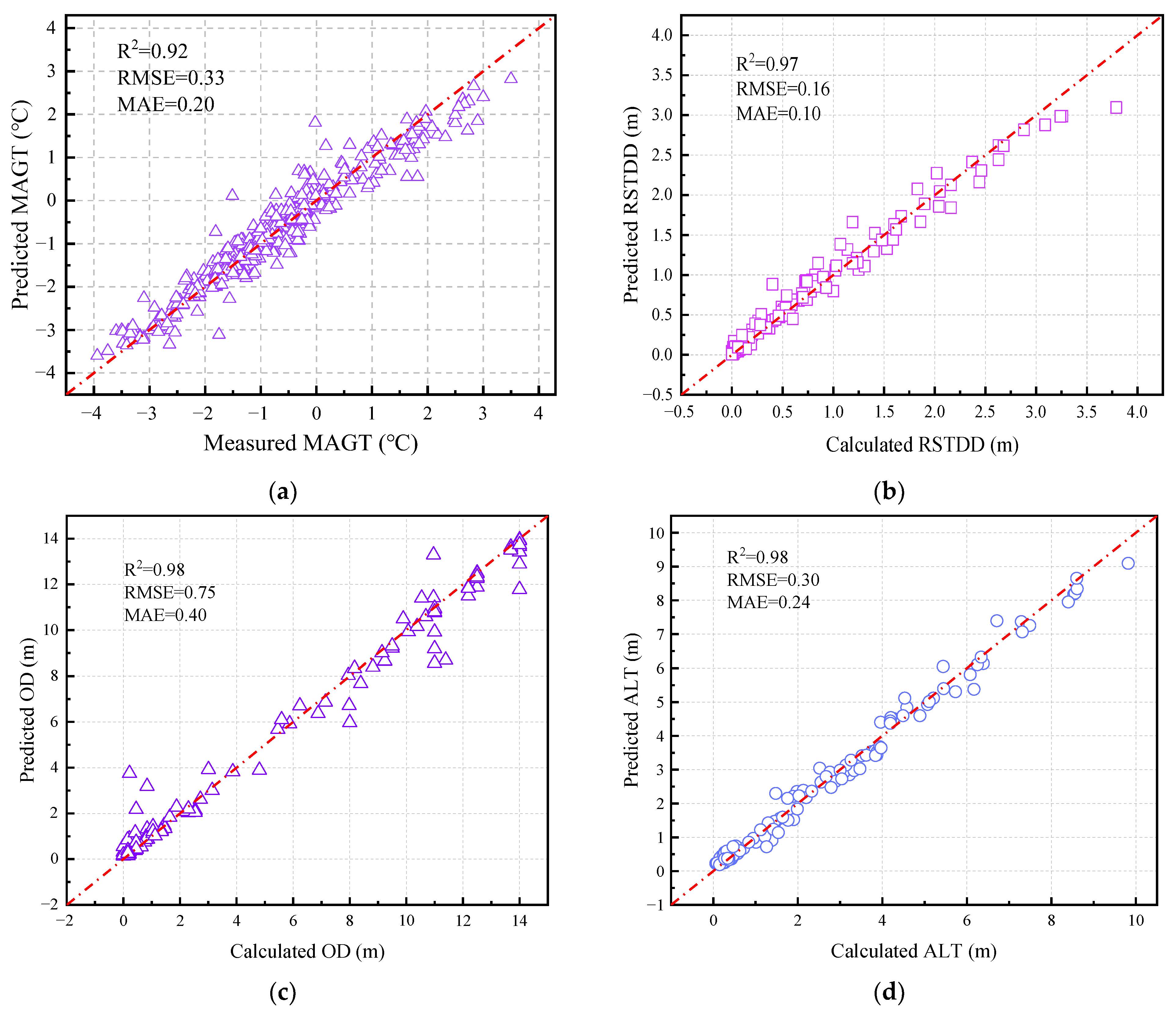
2.3.3. Prediction Accuracy of RF Model
To check the prediction accuracy of the proposed RF model, three error analysis indexes, namely, determination coefficient (
R2), mean absolute error (MAE) and root mean square error (RMSE), were employed to evaluate the prediction results of MAGT, RSTDD, OD, and ALT. The calculation results are given in
Figure 11. It can be seen that the
R2 values for MAGT, RSTDD, OD, and ALT are 0.92, 0.97, 0.98 and 0.98, respectively, while the MAE is 0.2, 0.1, 0.4 and 0.24, and the RMSE is 0.33, 0.16, 0.75 and 0.3. The evaluation metrics of the RF model indicate its high reliability and good fitting effect for prediction of the spatial distribution characteristics of morphological indictors along the QTH.
4. Discussion
4.1. Analysis of RSTDD, OD, and ALTD Patterns and Mechanisms
Figure 18 illustrates the effects of subgrade orientation, embankment height, ice content, and MAGT on the three key indicators under standard working conditions with all other factors held constant. The standard working conditions were defined based on the most representative factor combinations observed along the highway, including a prevalent 3 m embankment height, more-ice permafrost, an MAGT of −1 °C, and an east–west orientation (0°), which demonstrated the most pronounced SSSE.
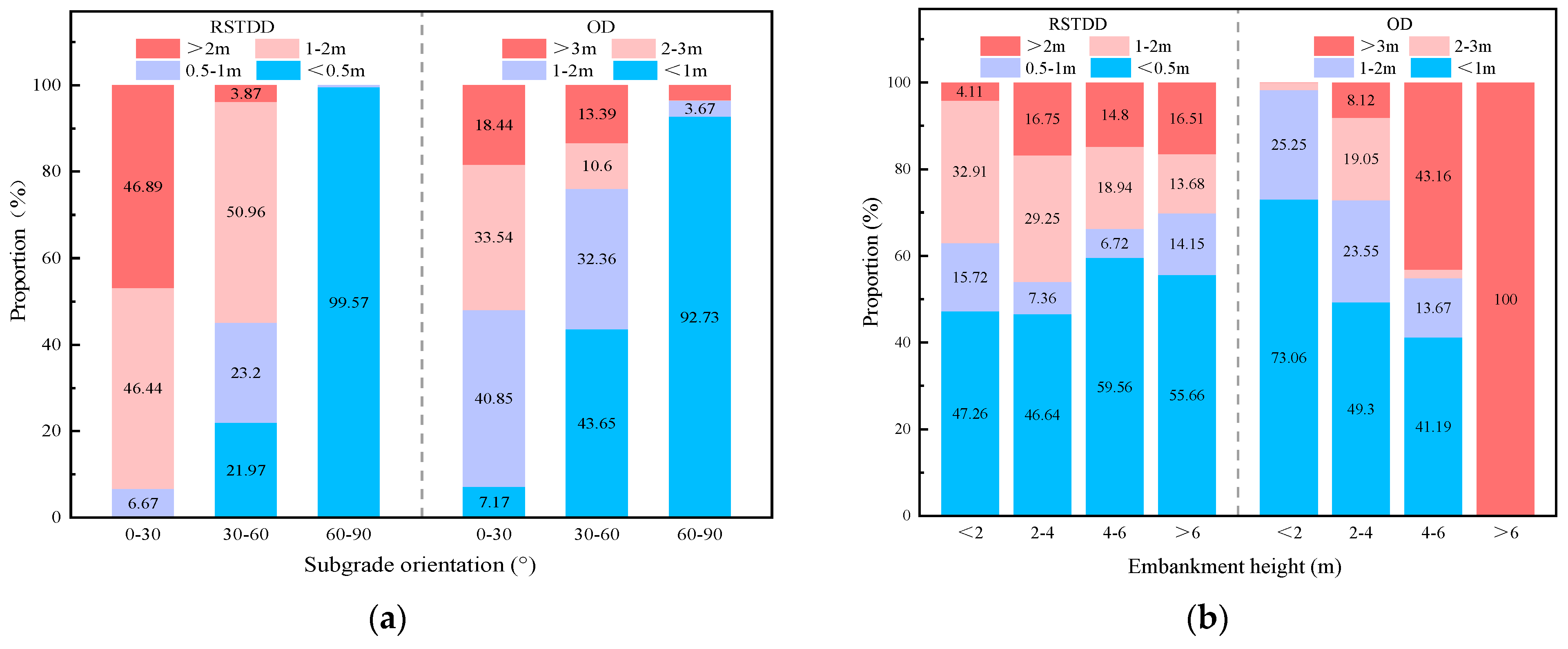
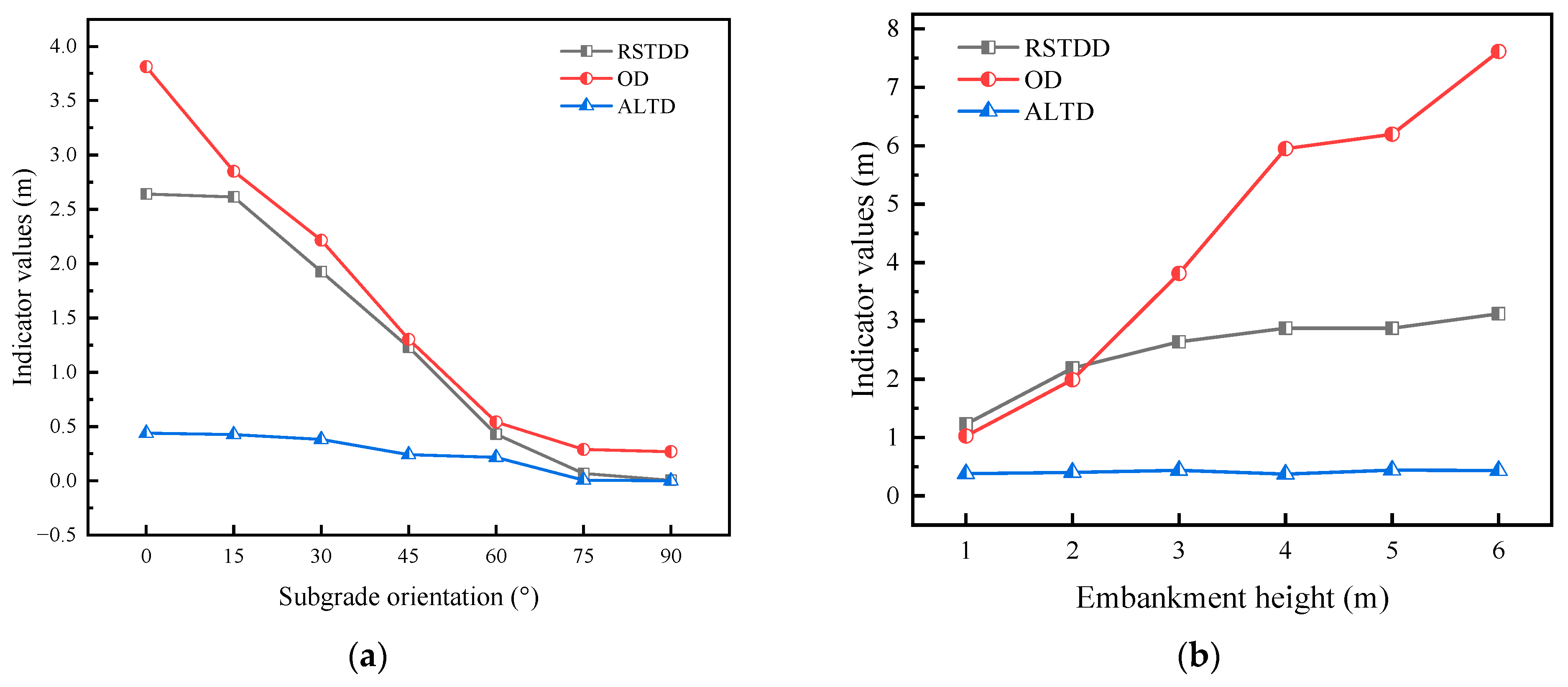
According to
Figure 18a, both the RSTDD and OD decrease as the subgrade orientation increases. Specifically, the RSTDD remains relatively stable at approximately 2.6 m within the 0–15° range; however, beyond 15°, its decline rate significantly accelerates, approaching zero at 75°. The OD reaches its maximum (4 m) at 0°, decreases rapidly with increasing orientation, and stabilizes beyond 75°. This is because the orientation directly regulates the differential solar radiation reception on sunny and shady slopes (Equations (4) and (5)). When the orientation is 0°, the maximum difference in heat reception between the sunny and shady slopes can reach 190 × 10
6 J. As orientation increases, this thermal contrast diminishes significantly, decreasing to 4 × 10
6 J at 75° and −0.1 × 10
6 J at 90°. Consequently, the SSSE becomes negligible.
According to
Figure 18b, both RSTDD and OD increase with embankment height, but their growth rate slows beyond 4 m, while OD exhibits a sharp increase at 6 m. This trend occurs because higher embankments increase the slope surface area, thereby amplifying the thermal disparity between the sunny and shady slopes. For example, compared to a 1 m embankment, a 6 m embankment results in a 23 × 10
6 J increase in the 20-year average thermal difference, corresponding to a 24.21% increase. However, the excessively high embankment height hinders the heat transfer to the deeper layers, resulting in the greatest thaw depth near the foot of the sunny slopes, so the offset varies drastically [
32,
33].
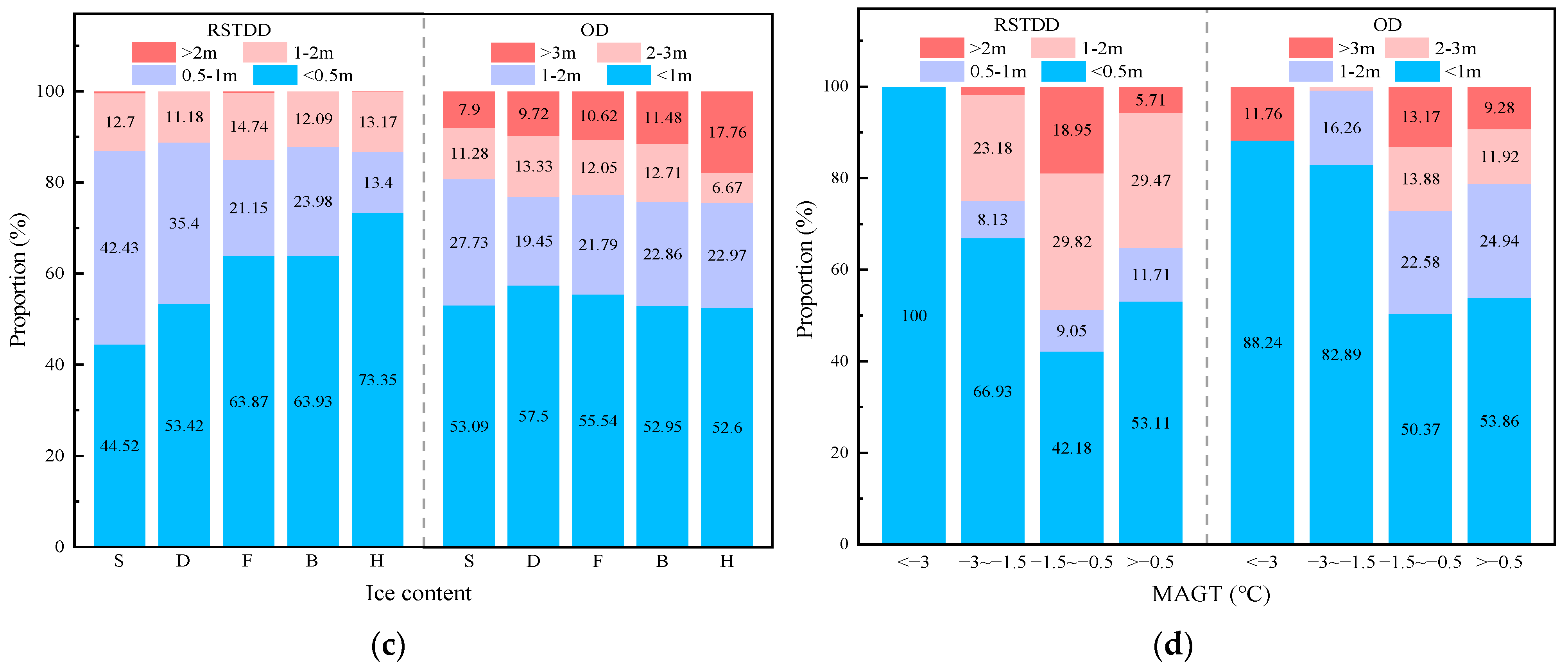
According to
Figure 18c, the RSTDD slightly decreases with increasing ice content, whereas the OD remains largely unaffected by ice content. The reason for this is that under natural conditions, high-ice-content permafrost exhibits a greater specific heat capacity; however, its lower natural density and higher thermal conductivity act as compensatory factors. This dynamic balance leads to relatively small variations in thermal diffusivity across different ice content levels. Consequently, the thermal response becomes more uniform, thereby weakening the influence of ice content on the morphological development of sunny–shady slope asymmetry.
As can be seen in
Figure 18d, the RSTDD shows a tendency of increasing and then decreasing with the increase in MAGT, and it reaches the maximum value at about −1.5 °C. This result is consistent with those from a previous study [
34]. In contrast, OD is not significantly affected by MAGT, likely because OD and ALTD are more influenced by local heat input heterogeneity and localized heat transfer processes, whereas MAGT does not directly modify the local solar radiation distribution or heat flux differentials.
In contrast, the ALTD remains relatively stable and is largely insensitive to these environmental factors. This stability can be attributed to the lateral heat diffusion and latent heat buffering effect of phase transitions [
35], which collectively limit heat penetration into deeper layers, thereby keeping ALTD at a consistently low level.
4.2. Impact Factors Weight Analysis
Table 6 ranks the importance of subgrade orientation, embankment height, ice content, and MAGT using the RF method. As shown in the table, subgrade orientation has the most significant impact on RSTDD with an importance of 49.84%. MAGT and embankment height also play crucial roles with importance values of 26.48% and 17.56%, respectively. MAGT is particularly influential in determining ALT with an importance as high as 80.58%, indicating that ground temperature is the primary controlling factor for ALT. The second most influential factor is embankment height with an importance of 10.44%. In contrast, OD is mainly influenced by subgrade orientation and embankment height with importance values of 51.80% and 35.82%, respectively.
To further validate the independence of model predictors, Pearson correlation analysis was conducted among subgrade orientation, embankment height, ice content, and MAGT. The results (
Table 7) show that while some predictors exhibit statistically significant correlations (e.g., embankment height and MAGT, r = –0.24,
p < 0.01), the overall correlation strength is weak (|r| < 0.30), indicating limited interdependence. Variance inflation factor (VIF) values for all variables are below 2 (
Table 6), confirming the absence of multicollinearity. From a thermophysical perspective, although predictors may interact through processes such as solar radiation redistribution, thermal buffering, and latent heat absorption, these interactions appear to be mitigated or canceled at the spatial and thermal resolution used. Therefore, treating the predictors as independent in the model structure is reasonable and does not compromise interpretability.
4.3. Limitations
Despite the valuable insights provided by this study, several limitations should be acknowledged, primarily concerning data quality, model assumptions, and the scope of simulation scenarios. The spatial resolution of the remote sensing data used, particularly MODIS land surface temperature with a resolution of 1000 m, is insufficient to resolve fine-scale thermal variations along the embankment slopes. This limits the model’s ability to accurately capture localized asymmetries in heat absorption and distribution, especially in terrains with strong microclimatic differences. Although terrain correction and calibration were applied, such coarse resolution may still overlook subtle but critical heterogeneities. Furthermore, ice content—a key parameter influencing permafrost thermal and mechanical behavior—was derived from the interpolation of borehole measurements. In regions with sparse sampling density, this may introduce considerable uncertainty, affecting the reliability of simulation outputs.
Another important limitation lies in the modeling framework adopted. While the two-dimensional earth–atmosphere coupled numerical model, integrated with an RF regression algorithm, demonstrated good predictive performance for asymmetric thaw morphology, it inevitably imposes simplifications on physical processes. The model does not explicitly resolve three-dimensional heat transfer or lateral moisture migration during freeze–thaw cycles, which are known to play important roles in permafrost degradation and thaw-induced deformation. Moreover, the RF model, being purely data-driven, lacks intrinsic physical interpretability, making it difficult to directly relate output importance rankings to governing thermodynamic mechanisms. Although useful for large-scale predictions, such limitations constrain the model’s ability to simulate process-based feedbacks or extrapolate to non-observed boundary conditions.
The scope of simulation scenarios considered in this study was also restricted. The numerical experiments were based on idealized embankment geometries and assumed a linear climate warming trend without incorporating the effects of variable snow cover, surface water pooling, or engineered interventions such as insulation layers or heat pipes. Furthermore, extreme climate events—such as rapid warming pulses or intense precipitation—were not accounted for, although they can have significant short-term and long-term impacts on permafrost stability. These simplifications, while necessary to ensure computational tractability and isolate key mechanisms, limit the model’s applicability under future climate variability and diverse engineering conditions.
Future research should aim to overcome these limitations by incorporating high-resolution datasets derived from UAV thermal infrared surveys, advanced satellite imagery, and dense ground-based monitoring networks to improve model fidelity. Extending the existing 2D framework into 3D coupled thermo-hydro-mechanical models would enable the more realistic simulation of lateral heat fluxes and deformation patterns. Moreover, the inclusion of more comprehensive boundary conditions—such as transient meteorological forcing, engineered subgrade treatments, and stochastic climate perturbations—will enhance the model’s robustness and practical applicability to infrastructure resilience planning in permafrost regions.


 ,
, 

