Evolution of Rockfall Based on Structure from Motion Reconstruction of Street View Imagery and Unmanned Aerial Vehicle Data: Case Study from Koto Panjang, Indonesia

Abstract

This study explores the growing application of 3D remote sensing in geohazard studies, particularly for rock slope monitoring. It highlights the use of cost-effective Street View Imagery (SVI) and Unmanned Aerial Vehicles (UAV) through Structure-from-Motion (SfM) photogrammetry as tools for 3D rockfall monitoring. Using multi-temporal SVI and UAV Imagery from the Koto Panjang cliff in Indonesia, we quantify rockfall volume changes over seven years and assess associated geohazards. The results reveal a total rockfall retreat of 5270 m³, with an average annual rate of 7.53 m³/year. Structural analysis identified six major discontinuity sets and confirmed inherent instability within the rock mass. Kinematic simulations using SVI and UAV-derived data further assessed rockfall trajectories and potential impact zones. Results indicate that 40% of simulated rockfall deposits accumulated near existing roads, with significant differences in distribution based on scree slope angles. This emphasizes the role of scree slope in influencing rockfall propagation. In conclusion, SVI and UAV imagery presents a valuable tool for 3D point cloud reconstruction and rockfall hazard assessment, particularly in areas lacking historical data. The study showcases the effectiveness of using SVI and UAV imagery in quantifying historical past rockfall volume and identifies critical areas for mitigation strategies, highlighting the importance of scree slope angle in managing rockfall hazard.

1. Introduction

Geohazard investigations increasingly rely on three-dimensional remote sensing techniques, as they can effectively capture the shape and changes in natural hazards, such as mass movements, lava flows, and debris flows, by comparing 3D point clouds acquired at different times [1]. These techniques are particularly useful in quantifying the evolution of rock slopes, including rockfall rates and deformation before failure, through the use of lidar technology [2,3,4] and point clouds obtained from photogrammetric methods [5,6,7,8,9,10].

The process of investigating rockfall changes can utilize technologies such as LiDAR [11,12,13] and UAVs with Structure from Motion (SfM) [5,7,8,14]. Those two methods yield point clouds, which are characterized by x, y, and z coordinates portraying a subject by representing it through a series of points. Point clouds that can reach centimeters [2] to sub-centimeter [15] resolution (i.e., point spacing) possess the potential to delineate topography with high precision, depending on the quality of the acquisitions. Through the quantitative analysis and comparison of topographic information acquired at distinct points in time, it becomes feasible to discern and gauge modifications associated with terrestrial surface processes [6].

Street view imagery (SVI) services, which provide 360° panoramas from various roads, streets, and locations worldwide, constitute a significant portion of the vast array of online images [16]. Street view images can be accessed through several providers such as Google Maps/Google Earth Pro [17], Apple Maps, Mappilary, Karta View, Baidu Maps, and Tencent Street View [16,18]. In most cases, panoramic imagery is acquired using a car mounted with multiple cameras, accompanied by various sensors, including LiDAR, though backpack-mounted cameras are also used for surveying narrow roads [19]. In this study, we utilized Google Street View (GSV) as our data services provider. Initially, GSV was primarily used in urban areas for virtual street navigation. However, its use has since expanded to include non-urban areas, allowing us to assess the slope hazard rate through imagery [20] and to detect and quantify volume changes due to rock failures [21].

This research aims to illustrate that 3D models generated from street view images and UAV imagery can not only aid the identification of changes in the landscape of rock slopes but also reveal the evolutionary patterns of a rock cliff throughout the documented year in a region where regular surveying and monitoring systems for rockfall hazards are not in place.

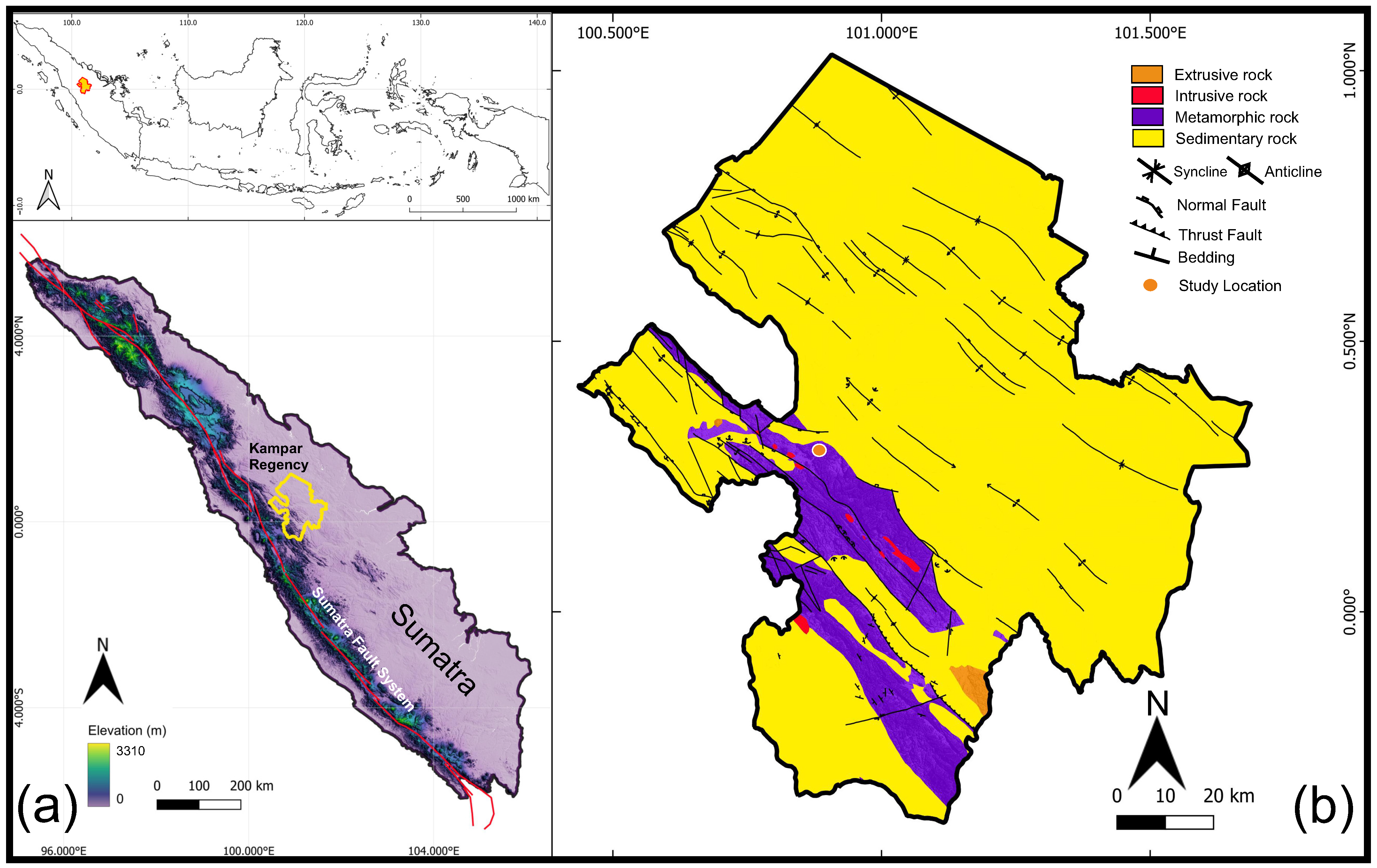
2. Geological and Geographical Setting

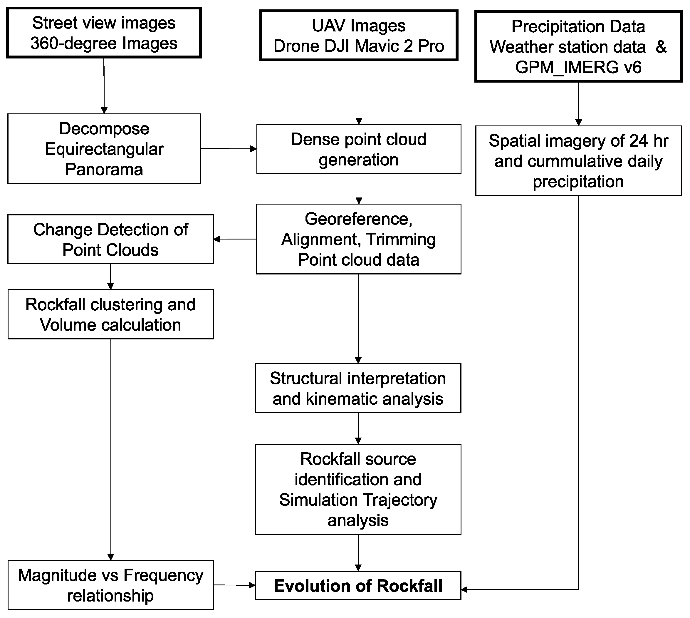
The study site is at KM 77 of the highway that connects the Riau and West Sumatra provinces, located within the Kampar Region of Riau Province, Sumatra Island, Indonesia (Figure 1). The studied rock cliff spans 170 m laterally and stands 25 m high, adjacent to the highway to the north and the Kampar River to the south. Three rockfall occurrences were documented in 2015, 2016, and 2019, obstructing the road. As a result, the economic route linking the Riau and West Sumatra provinces was adversely impacted (Figure 2).

The study site is part of the Bahorok Formation, composed of pebbly mudstone deposited in the Carboniferous–Early Permian [22]. This formation is mainly composed of non-bedded medium to coarse-grained breccioconglomeratic wackes [23]. Moreover, the Bohorok Formation has generally been affected by low, slate-grade, and metamorphism [24]. Subordinate interbedded mudstones, siltstones, quartzose arenites, and limestones are also present. These pebbly mudstones have a silt to fine sand-grade matrix. Their clasts are angular to subrounded, and clast lithologies indicate a continental source; vein quartz, argillites, and arenites are dominant among less common limestones, mica schist, and granite. Gneiss, chloritic schist, greenish calcsilicate rocks, and possibly rhyolite also occur. Fresh angular microcline is prominent in thin section [25].

The main structural feature on the island of Sumatra is the Sumatra Fault System, which was initiated in the Mid-Miocene. It was formed due to various superimposed tectonic events, including the widening of the Andaman Sea to the northwest of Sumatra and the extension of the Sunda Strait to the southeast of Sumatra in ±11 Ma [26,27]. Additionally, it is also associated with the oblique subduction of the Indo-Australian plate beneath the Eurasian plate [28,29,30] at a rate of 7 cm/year [31]. The Sumatra Fault System is characterized by broad, sinusoidal faults with lengths on the order of ten kilometers [26]. Structures in the Kampar Regency mainly trend northwest–southeast and northeast–southwest. Fractures in the area comprise dextral strike-slip faults and normal faults. Also, it has an average persistence of five fractures/meter with mostly joints and veins [31].

Figure 1. (a) Location of study site at KM 77 of the Riau-West Sumatra route in Kampar Regency, Riau, Indonesia. (b) Simplified geological situation of site, which predominantly consists of metamorphic rock and northwest–southeast trending structures (modified after [32]).

Figure 1. (a) Location of study site at KM 77 of the Riau-West Sumatra route in Kampar Regency, Riau, Indonesia. (b) Simplified geological situation of site, which predominantly consists of metamorphic rock and northwest–southeast trending structures (modified after [32]).

Figure 2. (a) Oblique 3D view of an aerial photograph of the study area (located within the red frame), modified from Google Earth and draped over an 8-meter digital elevation model (DEM). (b) Oblique aerial photo of the study site, captured using a DJI Mavic Pro 2 UAV in July 2021.

Figure 2. (a) Oblique 3D view of an aerial photograph of the study area (located within the red frame), modified from Google Earth and draped over an 8-meter digital elevation model (DEM). (b) Oblique aerial photo of the study site, captured using a DJI Mavic Pro 2 UAV in July 2021.

3. Methodology

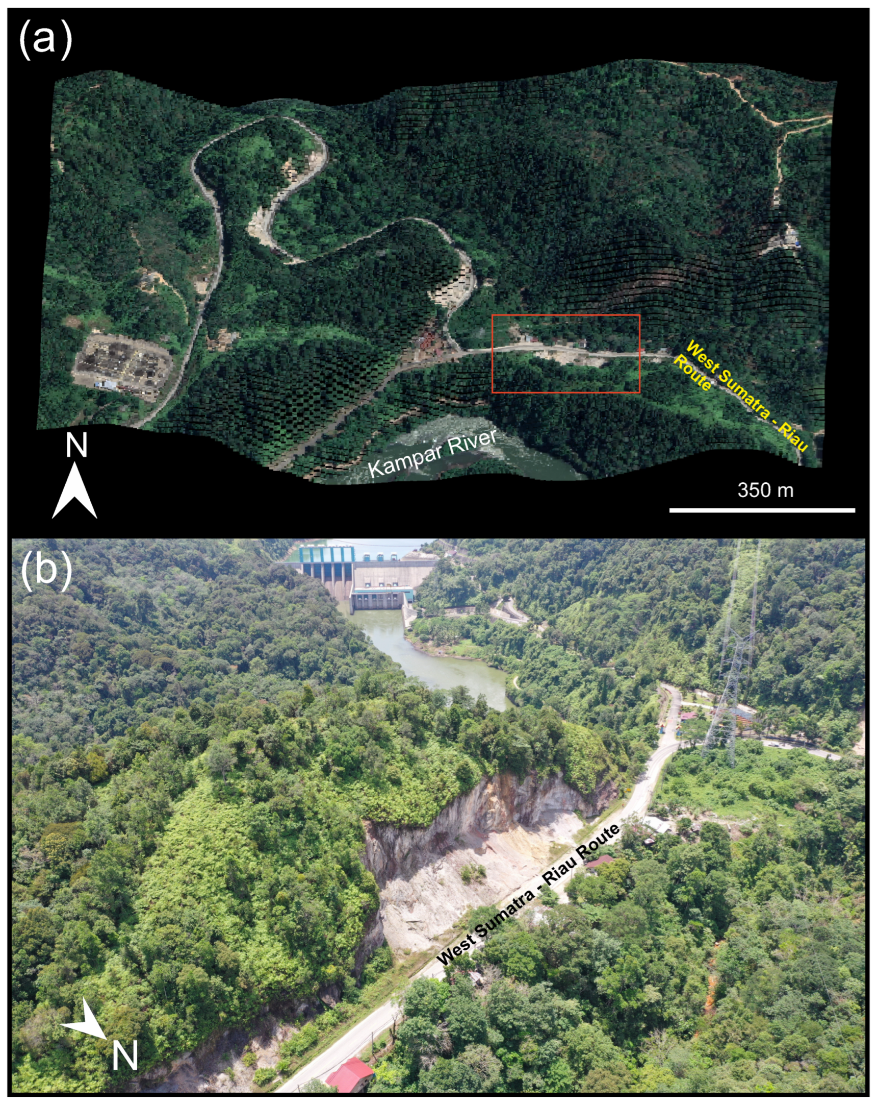
3.1. Image Acquisition

Two types of images were used in this study, from which 3D point clouds of the studied rock face were generated: Google Street View panoramas (i.e., SVI) and images captured using a digital camera mounted on an Unmanned Aerial Vehicle (UAV) (

Table 1. List of images retrieved from street view imagery and acquisition of UAV.

Time of Acquisition (MM.YYYY)	No. of Images	Acquisition Method
12.2015	26	SVI
12.2017	19	SVI
08.2018	26	SVI
10.2018	28	SVI
01.2021	36	SVI
10.2021	280	UAV

). Street view panoramas were accessed and downloaded through the Google Street View Static API [33,34]. The data have been historically collected by GSV from 2015 using monthly accuracy, and they continued to be captured yearly for up to seven consecutive years, ending in 2021.

In 2021, image acquisition was conducted using an unmanned aerial vehicle (UAV) equipped with a DJI Mavic 2 Pro. The UAV was fitted with a high-resolution camera capable of capturing images at 5472 × 3648 pixels, ensuring detailed and precise data collection. The point clouds generated from these UAV images were subsequently utilized for the calibration of point clouds derived from the SVI (Street View Imagery). This calibration process aimed to enhance the accuracy and consistency of the spatial data obtained from both sources.

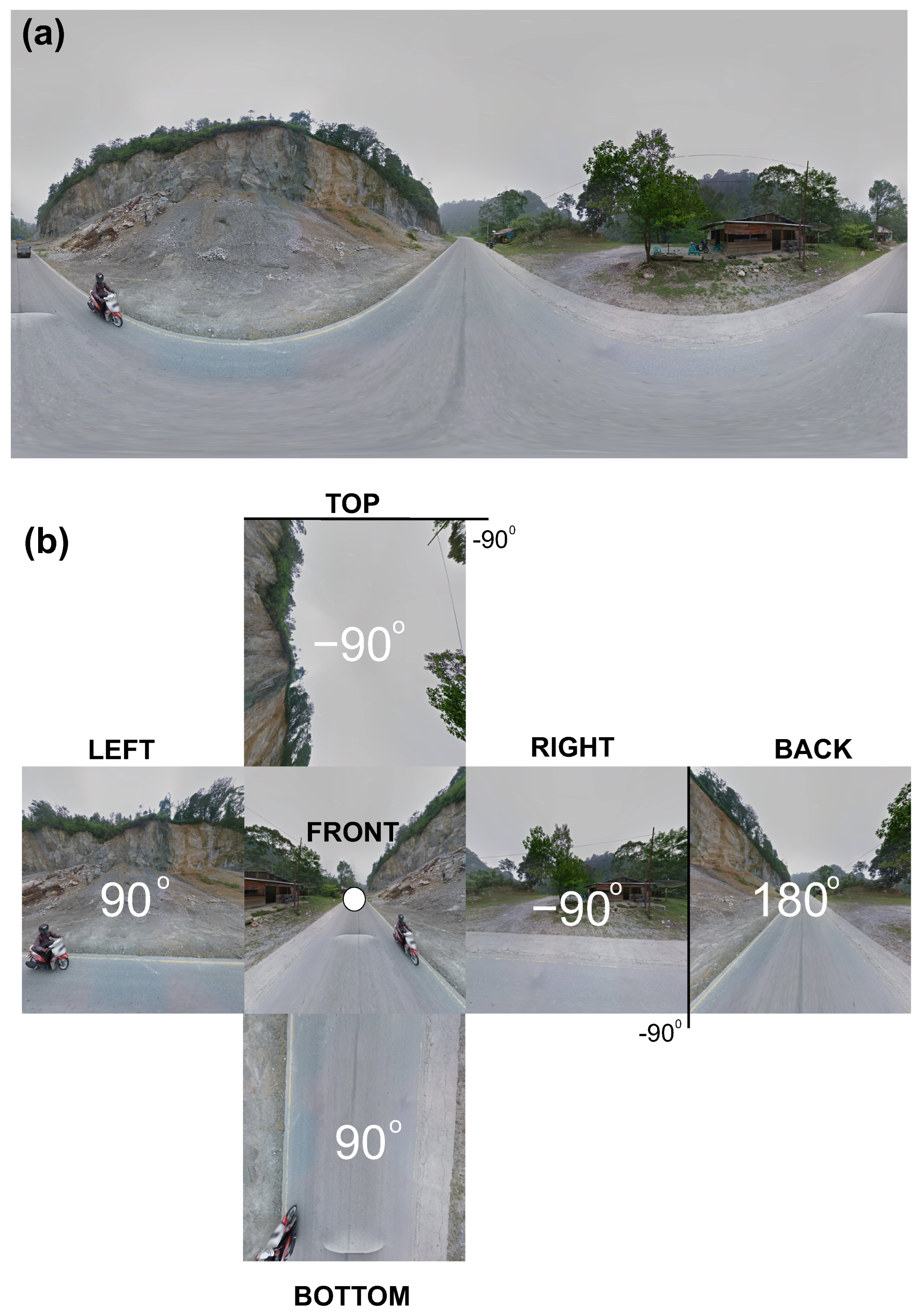
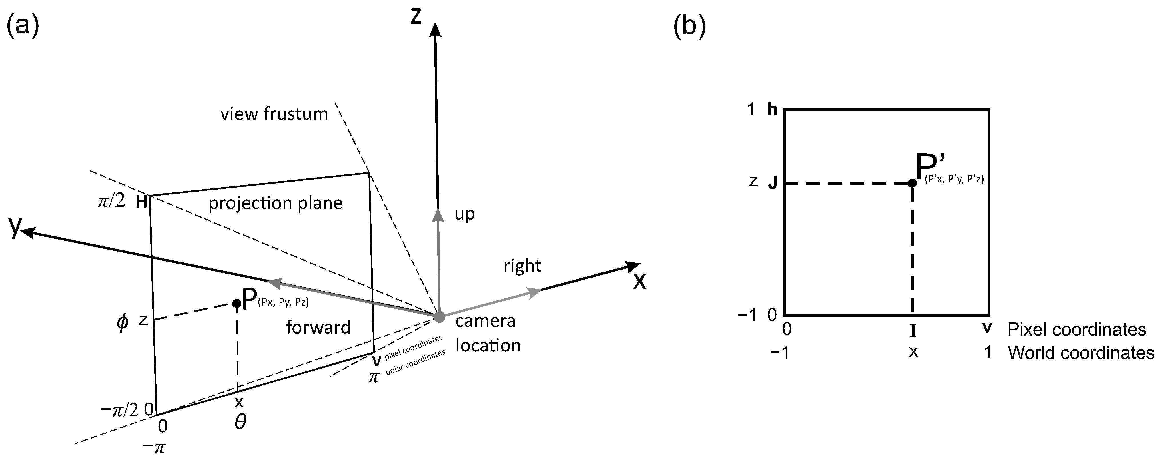
3.2. Decomposing 360-Degree SVI Images

Panoramic SVI (i.e., equirectangular images; Figure 3a) were converted into perspective images (i.e., cube faces; Figure 3b), which are more suitable for further processing into 3D point clouds using a structure-from-motion (SfM) workflow. These high-quality 360-degree SVI (Table 1) were decomposed using a MATLAB script [35] that converted equirectangular images into six cube faces with a resolution of 3328 × 3328 pixels per cube face image (Figure 3). The process of deriving cube maps from equirectangular images followed the method of Bourke [36].

The process begins by taking an equirectangular image as input. The width and height of this image are used to determine the size of the output cubic faces. If no specific output size is provided, a default size is calculated based on the width of the input image. Additionally, a vertical field of view (VFOV) is defined, determining how much of the spherical projection is visible in each face of the cube. By default, the VFOV is set to 90°. Each face of the cube corresponds to a specific direction: front, right, back, left, top, and bottom (see

Table 2. Cube face and rotation view from initial camera images.

Cube Face	Rotation
front	-
left	Pan by 90 degrees
right	Pan by −90 degrees
back	Pan by 180 degrees
top	Tilt by −90 degrees
bottom	Tilt by 90 degrees

). To define these directions, the function uses three angles: yaw, pitch, and roll. These angles describe how the cube face is oriented relative to the equirectangular image.

To project an equirectangular image onto the faces of a cube, the process begins by defining the point $\mathbf{P}$ as the top-left coordinate origin. This point serves as the reference for constructing the grid that will be mapped onto each cube face. The position of $\mathbf{P}$ (in Figure 4a) is determined by the vertical field of view (vfof) and the dimensions of the target cube face, as mathematically formulated in Equation (1).

$$\mathbf{P}=\left[\begin{array}{c}-tan\left({\displaystyle \frac{\mathrm{vfov}}{2}}\right)·{\displaystyle \frac{\mathbf{v}}{\mathbf{h}}}\\ -tan\left({\displaystyle \frac{\mathrm{vfov}}{2}}\right)\\ 1\end{array}\right]$$

(1)

Here, $\mathbf{v}$ and $\mathbf{h}$ denote the width and height of each cubic face, respectively.

A scaling factor $\mathbf{S}$ is derived to regulate the proportional spacing between grid points, as defined in Equation (2). This ensures the projected grid aligns precisely with the dimensions of the output cube face, preserving geometric accuracy during the mapping process.

$$\mathbf{S}=\left[\begin{array}{c}-{\displaystyle \frac{2·{\mathbf{P}}_{\mathrm{x}}}{\mathbf{v}}}\\ -{\displaystyle \frac{2·{\mathbf{P}}_{\mathrm{y}}}{\mathbf{h}}}\\ 0\end{array}\right]$$

(2)

where ${\mathbf{P}}_{\mathrm{x}}$, ${\mathbf{P}}_{\mathrm{y}}$, ${\mathbf{P}}_{\mathrm{z}}$ denote the x-, y-, and z-coordinates of the top-left reference point $\mathbf{P}$. For each cube face, a grid of spatial coordinates is generated, corresponding to pixel positions on the output face. This grid is initially constructed as a 2D array but is flattened into a sequential list of points to streamline computational processing. The initial coordinates are then transformed using $\mathbf{P}$ and $\mathbf{S}$ to ensure precise alignment between the grid and the equirectangular image. This transformation process is mathematically defined in the equations below:

$${\mathbf{P}}_{\mathrm{init}}=\left[\begin{array}{c}{\mathbf{P}}_{\mathrm{x}}+{\mathbf{S}}_x·{\mathbf{X}}^T\\ {\mathbf{P}}_{\mathrm{y}}+{\mathbf{S}}_y·{\mathbf{Y}}^T\\ {\mathbf{P}}_{\mathrm{z}}+{\mathbf{S}}_z·\mathbf{1}\end{array}\right]$$

(3)

where ${\mathbf{S}}_{\mathrm{x}}$, ${\mathbf{S}}_{\mathrm{y}}$, ${\mathbf{S}}_{\mathrm{z}}$ denote the scaling factors for the x-, y-, and z-axis components, respectively. The vectors ${\mathbf{X}}^T$, ${\mathbf{Y}}^T$ represent horizontal and vertical coordinate vectors of the grid. The initial 3D positions of the grid points, denoted as ${\mathbf{P}}_{\mathrm{init}}$ are computed by combining the base coordinates of the reference point $\mathbf{P}$ and the scaled grid $\mathbf{S}$.

Since each cube face requires a distinct spatial orientation, rotation matrices are applied to achieve alignment. Equation (4) defines the composite transformation matrix for each face, constructed from Euler-angle rotations: ${\mathbf{R}}_{\mathbf{x}}\left(\alpha \right)$ (pitch), ${\mathbf{R}}_{\mathbf{y}}\left(\beta \right)$ (yaw), ${\mathbf{R}}_{\mathbf{z}}\left(\gamma \right)$ (roll). This matrix rotates the grid points to match the target orientation of the cube face, ensuring seamless correspondence with the equirectangular projection.

$${\mathbf{R}}_{\mathbf{x}}\left(\alpha \right)=\left[\begin{array}{ccc}1& 0& 0\\ 0& cos\left(\alpha \right)& -sin\left(\alpha \right)\\ 0& sin\left(\alpha \right)& cos\left(\alpha \right)\end{array}\right]$$

$${\mathbf{R}}_{\mathbf{y}}\left(\beta \right)=\left[\begin{array}{ccc}cos\left(\beta \right)& 0& sin\left(\beta \right)\\ 0& 1& 0\\ -sin\left(\beta \right)& 0& cos\left(\beta \right)\end{array}\right]$$

$${\mathbf{R}}_{\mathbf{z}}\left(\gamma \right)=\left[\begin{array}{ccc}cos\left(\gamma \right)& -sin\left(\gamma \right)& 0\\ sin\left(\gamma \right)& cos\left(\gamma \right)& 0\\ 0& 0& 1\end{array}\right]$$

The transformation matrix $\mathbf{T}$ for each cube face is computed as the product of Euler-angle rotation matrices:

$$\mathbf{T}={\mathbf{R}}_{\mathbf{y}}\left(\alpha \right)·{\mathbf{R}}_{\mathbf{x}}\left(\beta \right)·{\mathbf{R}}_{\mathbf{z}}\left(\gamma \right)$$

(4)

Then, The transformed 3D coordinates ${\mathbf{P}}^{\prime }$ (see in Figure 4b), is achieved by applying T to the initial points ${\mathbf{P}}_{\mathrm{init}}$:

$${\mathbf{P}}^{\prime }=\mathbf{T}·{\mathbf{P}}_{\mathrm{init}}$$

(5)

After transformation, the points ${\mathbf{P}}^{\prime }$ are repositioned in 3D space and decomposed into their cartesian components ${\mathbf{P}}_{\mathbf{x}}^{\prime }$, ${\mathbf{P}}_{\mathbf{y}}^{\prime }$, and ${\mathbf{P}}_{\mathbf{z}}^{\prime }$. These components correspond to positions on the unit sphere represented by the equirectangular image.

The next step converts the 3D Cartesian coordinates to spherical coordinates, as defined by Equations (6) and (7). Here, each point is parameterized by two angles: the azimuth $\theta$, which measures the horizontal direction around the sphere (left/right), and the $\varphi$, which measures the vertical direction above/below the equatorial plane (up/down).

$$\theta =atan2\left({\displaystyle \frac{{\mathbf{P}}_{\mathbf{z}}^{\prime }}{{\mathbf{P}}_{\mathbf{x}}^{\prime }}}\right)$$

(6)

$$\varphi =atan2\left({\displaystyle \frac{{\mathbf{P}}_{\mathbf{y}}^{\prime }}{\sqrt{{\mathbf{P}}_{\mathbf{x}}^{\prime \mathbf{2}}+{\mathbf{P}}_{\mathbf{z}}^{\prime \mathbf{2}}}}}\right)$$

(7)

These angles are then mapped to pixel coordinates in the equirectangular image. The mapping ensures that each point on the cube face corresponds to the correct location in the equirectangular image as following Equations (8) and (9):

$$\mathbf{I}={\displaystyle \frac{\mathit{V}}{\mathbf{2}}}·\left(\mathbf{1}+{\displaystyle \frac{\mathit{\theta }}{\mathit{\pi }}}\right)+\mathbf{1}$$

(8)

$$\mathbf{J}={\displaystyle \frac{\mathit{H}}{\mathbf{2}}}·\left(\mathbf{1}+{\displaystyle \frac{\mathit{\varphi }}{\mathit{\pi }\mathbf{/}\mathbf{2}}}\right)+\mathbf{1}$$

(9)

where ($\mathbf{I}$, $\mathbf{J}$) represent new horizontal and vertical pixel coordinates for the cube face, and ($\mathbf{V}$,$\mathbf{H}$) denote the width and height of the equirectangular image in pixels. The azimuth angle $\theta$, which spans $[-\pi ,\pi ]$, defines the horizontal position around the sphere, while the elevation angle $\varphi$, bounded between $-\pi /2$ and $\pi /2$, determines the vertical position relative to the equatorial plane. The scaling terms $\pi$ and $\pi /2$ normalize the angular ranges to the pixel dimensions of the output image.

After all cube-face images were generated, geospatial coordinates were embedded into the images using the ExifTool library [37].

3.3. Data Processing

3.3.1. Dense Points Cloud Model Generation

The process for image datasets of SVI in Kotopanjang is only three out of six image cubes, which represent part of the road and rock cliff. All the selected photographs from SVI and UAV were processed using Agisoft Metashape Professional (version 1.5.4) SfM-MVS (Multi-View Stereo) software [38]. Graber and Santi (2023) [6] explain the general process of creating 3D point clouds from images using Agisoft Metashape, which involves initial photo screening and importing, photo alignment and tie point selection, trimming of the sparse point cloud, optimization of the camera alignment, and creation of a dense, high-quality point cloud.

3.3.2. Georeferencing and Registration of 3D Model

Five point clouds generated from GSV images and one point clouds generated from UAV images were imported into the CloudCompare (version 2.12 alpha) software package for alignment and analysis. These 3D point clouds were aligned (i.e., co-registered) with a reference point cloud extracted from the national Digital Elevation Model (DEMNAS), which has a resolution of 8 m per pixel. Preliminary alignment (i.e., coarse alignment) was performed by choosing a minimum of three pairs of points based on their features from the entire 3D point cloud.

Alignment of the point clouds was further improved using the Iterative Closest Point (ICP) algorithm [39], which minimized the root mean square error (RMSE) between the point clouds. Before applying the ICP technique, we marked two areas that were considered to be stable. The stabilization of the remaining sections of the datasets, initially considered unstable, was achieved using the transformation matrix derived from the first step. The Poisson Surface Reconstruction algorithm [40] was then employed to produce a 3D mesh [40].

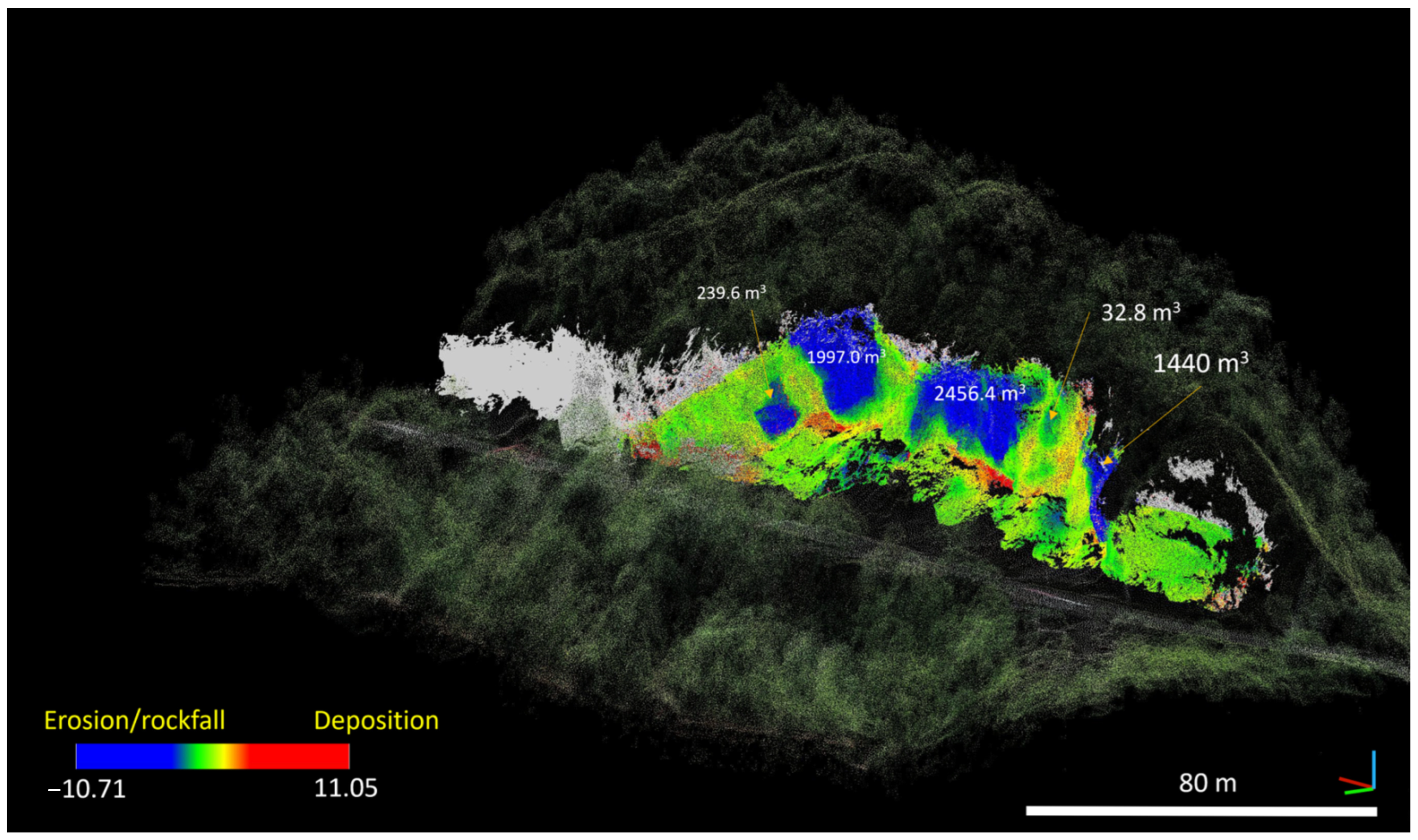
3.3.3. Change Detection of Point Clouds

We used the M3C2 plugin [41] within CloudCompare [42] to detect change between the point clouds. The cylindrical neighborhoods were oriented using the normal vectors obtained during the SfM processing instead of creating new ones. All of the points in point cloud following down sampling and cleaning in the pre-processing steps, served as ‘core points’ where the M3C2 calculation was carried out. Multiple neighborhood sizes (representing the cylinder’s diameter) were applied for each change detection interval to ensure the detection of both small and large changes. For the point clouds, we used neighborhood diameters of 0.3, 0.5, and 1.0 m. For every set of M3C2 distances, an empirical limit of detection (LOD) was determined by fitting a normal distribution to the M3C2 distance histogram. This process involved minimizing the sum of squared errors between the distance histogram and the normal distribution model. The empirical LOD was defined as the range within ±2 standard deviations from the mean M3C2 distance. M3C2 distances were computed between the initial and final scans for each slope to identify potential rockfalls throughout the monitoring campaign. After assessing the changes, alterations exceeding the empirical LOD were manually inspected to distinguish rockfalls from other factors such as erosion, missed vegetation, photogrammetric noise, or registration error. To confirm each rockfall source and to bracket the timing of each rockfall event as closely as possible, we reviewed all the photo datasets for the relevant locations where changes occurred [41].

3.3.4. Rockfall Clustering and Volume Calculation

In the process of validating each rockfall occurrence and pinpointing their timing with precision, the photo datasets relating to the specific areas where the changes took place were carefully analyzed. In cases where changes were unclear, the photo datasets were used to confirm their correlation with rockfall incidents. The examination of change plots and RGB photos served the purpose of pinpointing the locations linked to rockfalls [13]. Following that, we manually defined and separated the clusters of points linked to rockfall events. The rockfall volume calculation was conducted using the 3D alpha-shape method, as per the guidelines proposed by [7,43].

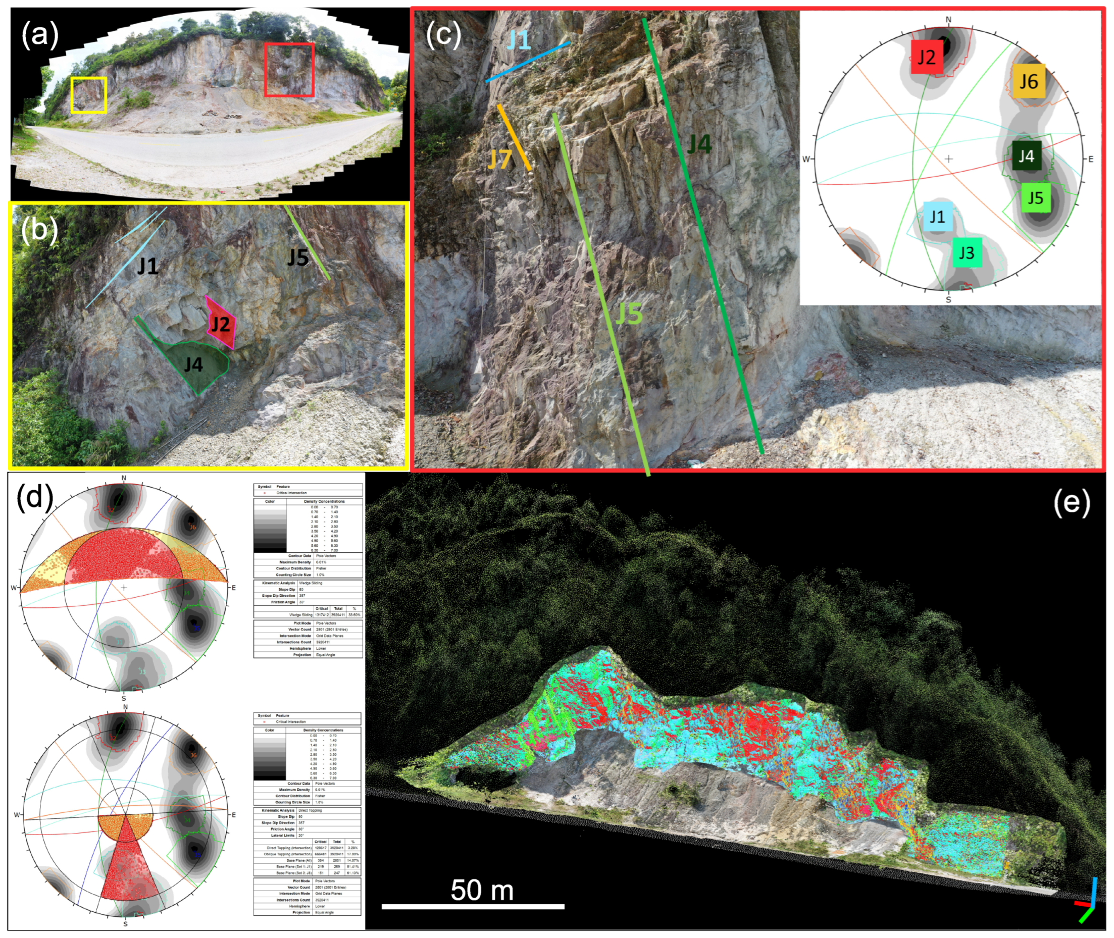
3.3.5. Structural Measurement and Kinematic Analysis

By utilizing georeferenced 3D point cloud data acquired through SfM photogrammetry and Coltop3D software [44], a 3D shaded, colored relief map was generated, with colors corresponding to the rock cliff orientation (slope aspect and angle) (Figure 5). These point clouds enabled topographic and structural analyses, which are critical to the study of rock slopes that are remote or difficult to access, making traditional field investigations challenging. To gain a better understanding of how discontinuities contribute to progressive slope failure, it is essential to determine the discontinuity sets involved in past events. Using the point clouds, we were able to identify the discontinuity sets associated with rock slope instability. Six primary joint sets (J1 to J6) were identified in the Coltop3D software. The point cloud of each discontinuity set was imported into CloudCompare, where it was compared with the locations of rockfall sources (interpreted from the point cloud of the rock cliff) [45]. This method allowed us to determine the number of rockfalls each joint set had been involved in.

Kinematic analysis is also provided by examining the potential movement of rock blocks on point clouds and is performed using DIPS and StnParabel software. This analytical approach is performed by identifying types of block failures, such as sliding, toppling, or falling, which can occur due to the orientation of geological discontinuities, including joints and faults.

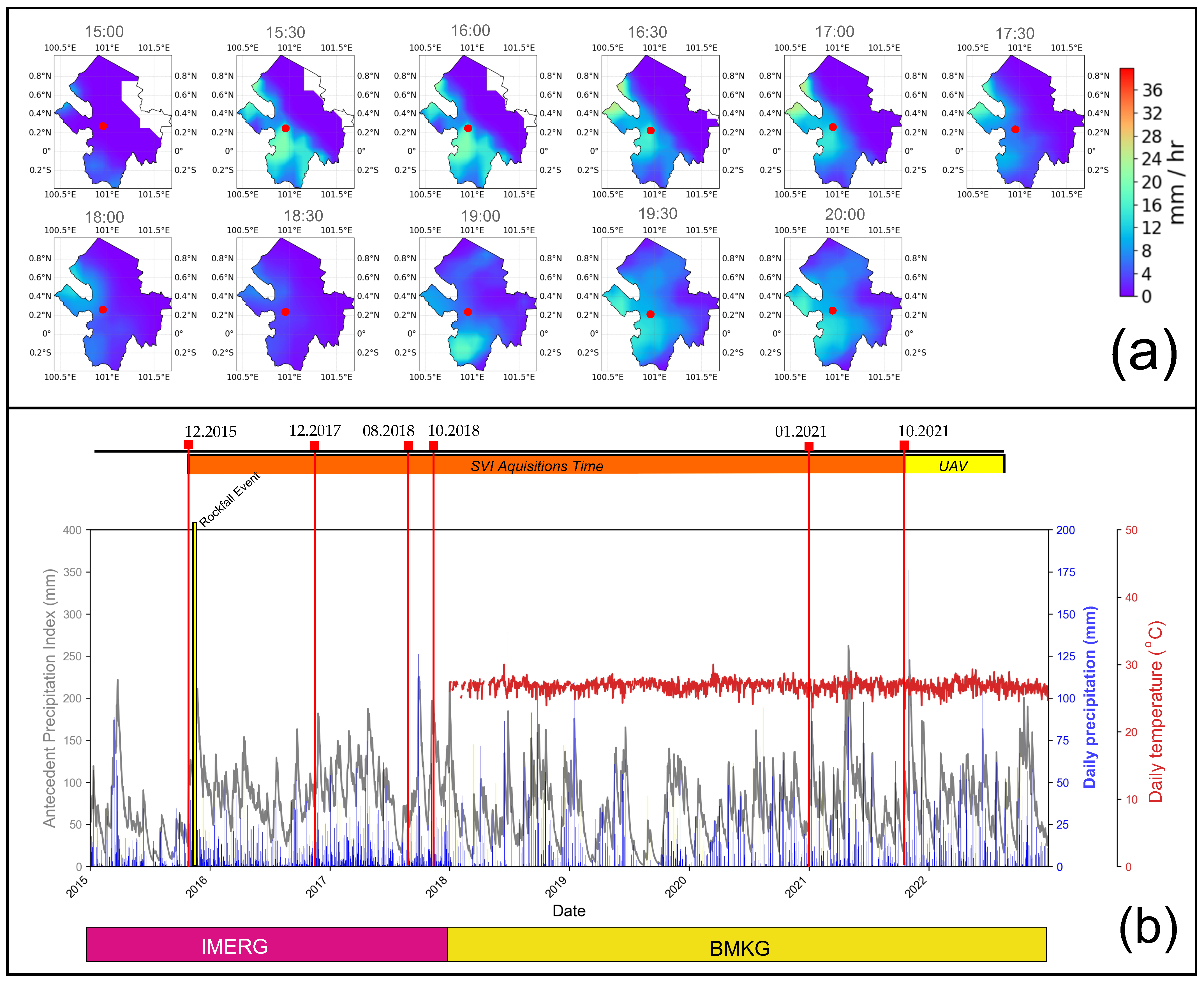
3.3.6. Precipitation Analysis

In analyzing precipitation data, two data sources were used—local weather station data from 2018 to 2023 and NASA Global Precipitation Measurement (GPM) data—using the Integrated Multi-satellite Retrievals for GPM (IMERG) algorithm to estimate precipitation over the majority of the Earth’s surface [46]. The analysis is performed by calculating the Antecedent precipitation index (API) [47].

$${\mathrm{API}}_t=\sum _{i=1}^n{P}_i·k^i$$

(10)

where ${\mathrm{API}}_t$ represents the Antecedent Precipitation Index at time t, $P_i$ denotes the precipitation amount i days before time t, k is the decay factor with a value between 0 and 1 ($0<k<1$), and n indicates the number of preceding days considered in the calculation. This analysis is overlaid with daily weather precipitation data, combined with temperature data plots. As for the GPM data, we selected the IMERG precipitation Half Hourly 0.1 degree × 0.1 degree V06 and IMERG precipitation day 0.1 degree × 0.1 degree V06 product, which provides more accurate precipitation information across Global Precipitation Climatology Centre (GPCC)-gauged regions compared to the near real-time products [46]. The data were selected based on rockfall events that occurred on 13 November 2016. These IMERG plot data are taken on rockfall events that occurred in 2016 because the weather station data do not cover data before 2018. Data processing is performed by extracting hdf5, which can be accessed on https://www.earthdata.nasa.gov/ (accessed on 11 June 2024) and taking daily and 24 h data every half hour. The data are calculated cumulatively daily and plotted by overlaying the study location points.

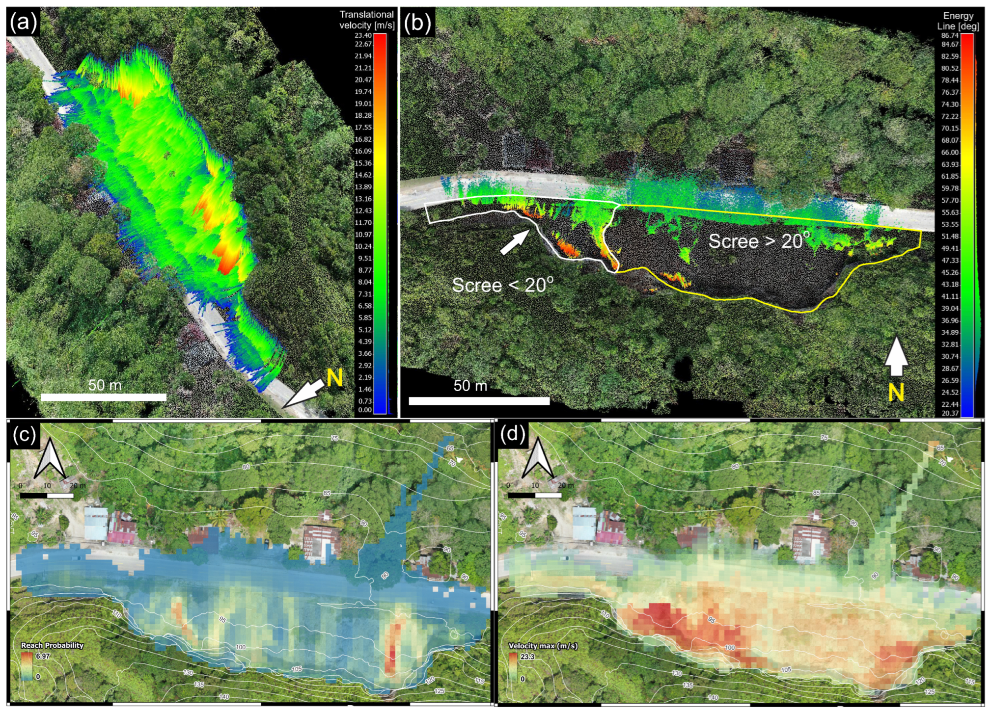
3.3.7. Trajectography Analysis

The simulation of the rockfall trajectories and impacts was performed with stnParabel [48], using the point cloud as topographic input. This algorithm takes into account the size and shape of the falling rock, the roughness of the terrain, the gravitational potential energy of the rock, air resistance, and frictional forces between the rock and the terrain. The software creates simulations of rockfalls to calculate specific values such as the source point, energy line, translational energy at impact, velocity, post-deposited trajectory in each 3D point information, and also provides raster results of reach probability, mean and maximum velocity, and mean and maximum elevation of trajectories.

For this simulation, the point cloud is used to represent the terrain over which the rockfall is simulated. For the data preparation, we used a set of data points in a 3D coordinate system that represents the surface of an object or terrain. In this case, the point cloud represents the terrain over which the rockfall is simulated. The detail of the point cloud spacing is defined depending on the size of the rock (as for the study, we used a 0.02 m point spacing). So the smaller size of the rock will be followed by the density of the point spacing between the point cloud [49]. We also used kinematic analysis for source identification using information from joint datasets in the software and integrated the results into the simulation [49]. An overview of the research study workflow can be seen in (Figure 5).

4. Results

4.1. Structural Interpretation

This scarp area shows a slope face oriented on average at $0^{°}$, with a dip slope up to ${80}^{°}$. The scarp has a length of 122 m, 27 m in height, with six main discontinuity sets (J1 to J6) that were identified from point cloud data and direct field measurements

Table 3. Dip direction and dip of planar discontinuities measured in the field and from point clouds (using Coltop3D).

Discontinuity Set	Dip Direction/Dip from Field Measurements (°)	Discontinuity/m	Dip Direction/Dip from Point Cloud Measurements (°)	Tolerance Angle
J1	$008/53$	5	$8/53$	±15.0
J2	$169/77$	5	$168/77$	±15.0
J3	$345/77$	5	$348/77$	±15.0
J4	$270/60$	5	$272/60$	±15.0
J5	$295/75$	5	$298/75$	±15.0
J6	$224/82$	5	$225/83$	±15.0

. J1 and J3 stand out as pervasive joint sets that are present along almost the entire outcrop. These sets are similarly oriented to regional fracture zones (Figure 6).

Based on the collected discontinuity and slope orientation data from the rockfall source zone. Although the orientation of discontinuity sets may slightly vary in different sections, a total of two dominant discontinuity sets (J1 and J3) were identified; $J1$: 8/053, $J3$: 345/77 (Figure 6). The friction angle of discontinuities in the rockfall source zone was calculated to be ${30}^{°}$. Based on the kinematic analysis performed for the rockfall source zone, it was determined that the most common discontinuity-controlled failure type in the source zone is the wedge and block toppling failure (Figure 6). This dominant discontinuity is attributable to its alignment with a regional fracture zone.

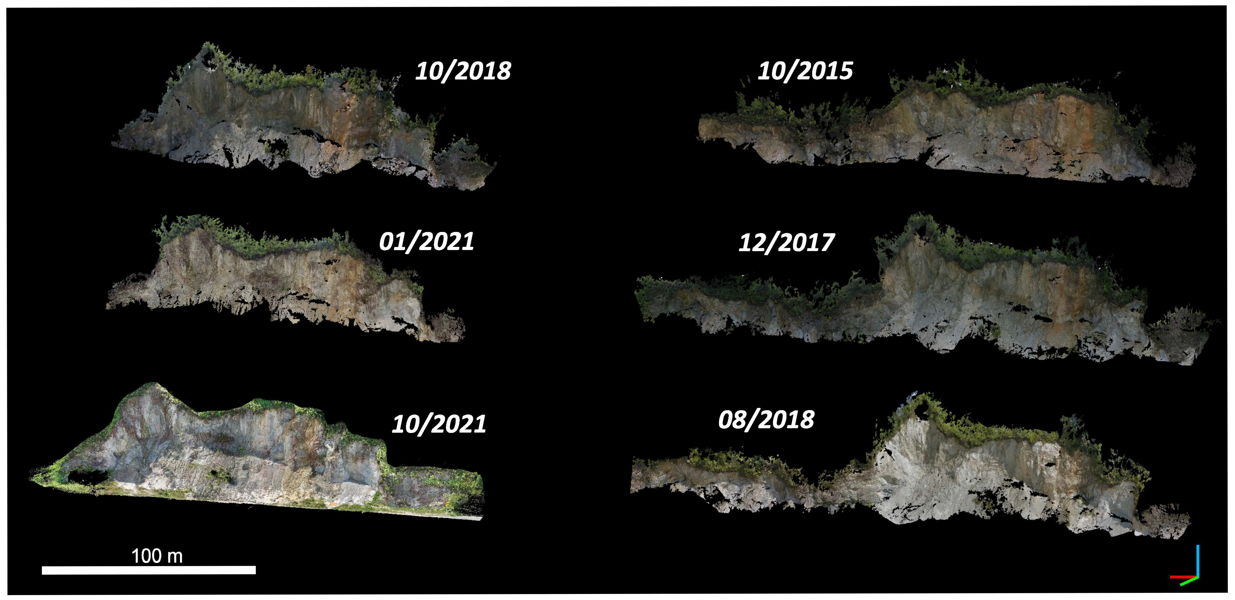
4.2. Comparison of Point Cloud Data

Based on the results of SVI and UAV data processing using Agisoft software, seven point clouds can each be processed and compared. The result covered all the cliff scarp in the area except for SVI from January 2019, which missed a section of the scarp (Figure 7).

The topography of the studied rock cliff appears to have changed significantly between 2015 and 2021 due to mining and rock collapse (Figure 8). By comparing the 3D point clouds from these years, 27 rockfall source areas are identified as sources of rockfall, with volumes ranging from 8 to 1774 m³, have been identified. Between October 2015 and December 2017, 11 rockfalls occurred, followed by seven rockfalls between December 2017 and October 2018 and 10 rockfalls between October 2018 and October 2021 (Figure 8). The cumulative rockfall volume from 2015 to 2021 was approximately 5.27 × 10³ m. On average, 3.85 rockfall events occurred annually, resulting in a total volume change of 7.53 m³ from 2015 to 2021.

The volume–frequency (V-F) relationship for rockfalls and rock fall sources volumes is distributed according to a power law [50]. Before 2015, no data were noted and recorded. This might make our estimates more cautious, leading to a calculated return period for rock failure that may differ from its actual frequency but align with the power law pattern. The relationship differs if we consider only the events from 2015 to 2021 or if we include two large events from 2016 and one from 2018. The corresponding power law fittings for 27 blocks retreat are as follows: $N(v\ge V)$ = 22.43 $V^{-0.63}$ obtained using least squares linear regression. In this case, the minimum, or cut-off, volume ($V_0$) of the power law fitting is set as 5.25 m³ (Figure 9).

Concluding that the scaling exponent b, crucial for assessing the frequency of rock failure events, is more significantly influenced by the maximum recorded rock failure volume in the historical inventory than by the minimum volume, and it achieved this by analysing both types of volumes through regression and using the scaling exponent b from published references [6,51]. The insufficient representation of large rock failure events in fitting the power-law tail profoundly impacts the ability to predict the frequency of future, more significant events. This underscores the importance of considering the maximum rock failure magnitude in the inventory to prevent unrealistic extrapolation and to accurately determine the frequency or return period of larger failure events.

4.3. Precipitation Analysis

A detailed analysis of GPM-IMERG data on 1 day before the event on (13 October 2016) reveals a surge in rainfall intensity starting on 15:00 until 20:00, with values ranging from 32 to 36 mm/day, and it lasted for 5 h. This substantial rainfall peak stands out prominently amidst the overall rainfall distribution for the day, accumulating to a total of 220–240 mm/day (Figure 10a). Meanwhile, based on daily precipitation data from the climatological weather, it shows the maximum API value of 189.33 mm and the lowest at 2.69 mm (Figure 10b). This indicates that there is an increase in rainfall just before the rockfall event at that time.

4.4. Trajectography Results

Upon analyzing the processed kinematic analysis data, we identified 1542 potential sources. Subsequent simulation parameters were conducted using a rolling friction algorithm for the impact model and a volume size of 1 × 1 m³, with 100 simulations performed for each point source. Detailed parameters are shown in (

Table 4. Parameter used for trajectography simulation.

Parameter	Value
3D terrain model	22,625,890 points
Friction Angle $\left({\phi }^{\prime }\right)$	${28}^{°}$
Cohesion $\left(c^{\prime }\right)$	30 kPa
Volume	1 m3
Density	2700 kg/m3
No. of Simulations	100 each sources

) and in 3D view perspective (Figure 11a).

The simulation results, based on the spatial overlap between (post-deposited) trajectories and infrastructure data, showed that approximately 40% accumulated at locations where roads and infrastructure were present, generating translational kinetic energy impacts with an average value of 52 kJ and a maximum value of 321 kJ. Additionally, the average energy line exhibited a value of ${46}^{°}$ (Figure 11d).

Particularly noteworthy is the differential distribution of deposited rockfall across sectors with scree slopes exceeding ${20}^{°}$ and those with slopes below ${20}^{°}$. This distinction underscores the significant impact of scree slope on rockfall trajectories. As evident from (Figure 11b), the eastern sector consistently exhibits a more extended trajectory compared to the western sector, demonstrating the pronounced influence of scree angle on rockfall distribution. This is also shown by the roughness in the eastern sector, which is higher due to active scree slope accumulated from rockfall events, while the western sector has already been excavated and has less accumulated rockfall, which tends to be more flat.

5. Discussion

5.1. Volume Calculation

While the identified discontinuity sets and orientations matched field observations, normal spacing remained unknown due to inaccessible rock faces. Utilizing 3D point cloud data and existing methods allowed for an objective estimation of normal spacing and, consequently, the detached block’s average volume. Factoring in this size provides more realistic travel distances and energies as the fallen block fragments along existing discontinuities [52].

Decomposing images from street view imagery could provide a solution in order to provide historical topography relief conditions, although it gives a lower detail resolution compared with recent technologies using UAV (

Table 5. Comparison of UAV and Street View Imagery.

Parameter	UAV Imagery	Street View Imagery
Perspective	Aerial (top-down), variable altitudes.	Ground-level (human-eye height), 360° panoramas.
Resolution and Detail	Sub-centimeter resolution; excels in overhead details (e.g., outcrops).	5–10 cm/pixel at ground level; captures horizontal features (e.g., hillsides, signs).
Coverage	Flexible: remote areas, off-road, hazardous zones.	Road-focused: urban/rural streets with vehicle access.
Data	Real-time updates possible; customizable frequency, Sufficiently generated visuals.	Historical archives available, often outdated (1–2+ years old), limited image availability.
Cost	Higher cost (USD 1k–USD 50 k with equipment, permits, skilled operators).	Free/low-cost (Google Maps, APIs); instant access to existing data.
Limitations	Regulatory hurdles, weather-dependent, short battery life (20–60 min).	Limited coverage (e.g., narrow alleys, private property), privacy blurring obscures details.
Strengths	High spatial accuracy, 3D modeling, dynamic monitoring.	Human-scale context, street visual analysis.

) or LiDAR. Since our result is also related to the volume calculation, which is carried out solely using the ICP (iterative closest point) method with UAV data, which has been calibrated and georeferenced with DEM data, it is still necessary to pay attention to the volume of the comparison results between point clouds that can provide a large enough standard deviation on the accuracy of the data used in the calculation of the magnitude frequency relationship graph [6,53].

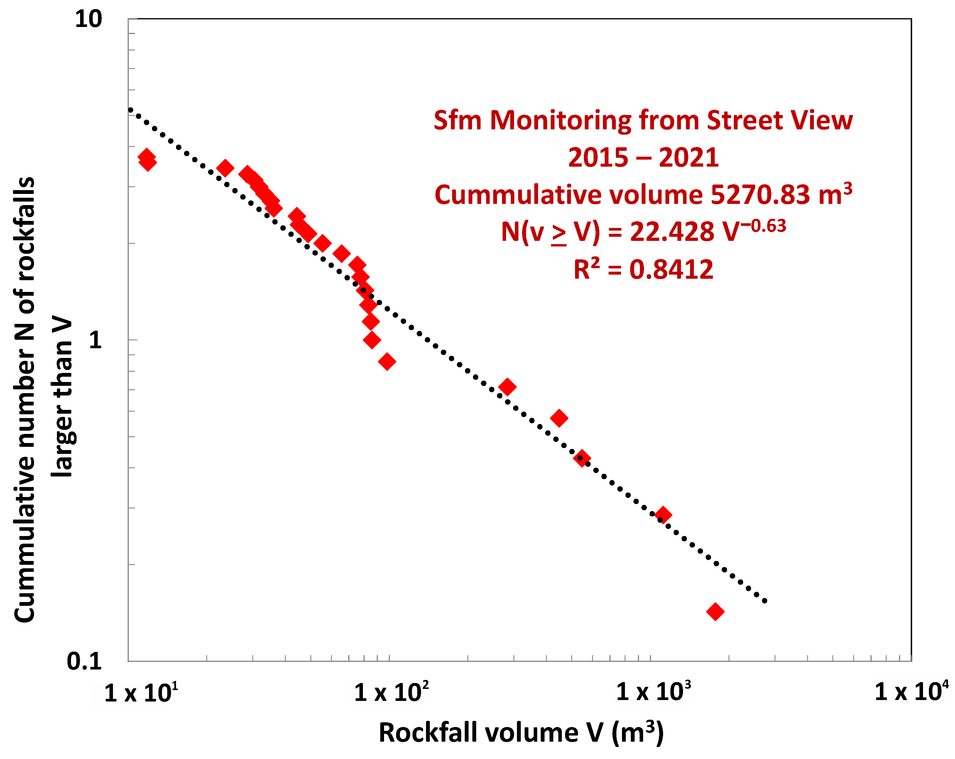
5.2. Rockfall Magnitude vs. Frequencies

The detected rockfall volumes—ranging from a minimum of approximately 5.25 m³ to a maximum of around 1700 m³ —suggest that the observed events fall within a relatively moderate size range. This volume spectrum indicates that the dataset is dominated by smaller-to medium-sized rockfalls, which are typically more frequent. Moreover, this result is still an insufficient representation of large rock failure events in fitting the power-law tail, and it profoundly impacts the ability to predict the frequency of future, more significant events [6].

The magnitude-frequency relationship of rockfalls is commonly modeled using a power-law distribution [54] expressed as

$$F_{st}=A_{st}{V}^{-B},$$

where $F_{st}$ denotes the spatiotemporal frequency of rockfalls exceeding a given volume V, $A_{st}$ is the activity parameter characterizing the frequency of rockfalls larger than one cubic meter, and B characterizes the scale invariance of the rockfall volume–frequency power law and reflects how uniformly rockfall volumes are distributed over the considered volume range.

Following the methodology outlined by Hantz [54], the uniformity parameter B can be estimated based on the rock mass structure description derived from field observations. Given the Geological Strength Index (GSI) of the study site, which indicates a blocky structure with non-massive rock conditions, the expected range for B falls in between 0.5 and 0.7. This estimate aligns with statistical regression of the magnitude-frequency relationship, which gives $B=0.63$ (see Figure 9). According to the method of Didier et al. [54], the order of magnitude of the activity parameter $A_{st}$ can be calculated using discontinuity spacing data, yielding a value of 0.2. However, based on our calculation using cliff geometry and the possible event of activity, it shows a value of 0.34. This comparison of $A_{st}$ shows the baseline frequency of rockfalls exceeding one cubic meter per year per hectare, showing reasonable coherence between theoretical results and field observations at the study site. Similarly, the comparison of B values demonstrates that the observed parameter values align well with theoretical expectations, supporting the reliability and consistency of the proposed methodology.

Since $V_{\max }$ often exceeds the largest observed volume in inventories, it is typically estimated using expert judgment informed by geological evidence such as the size of previous scars, deposits from former rockfalls, potentially unstable rock compartments, and cliff height [55]. In this case, the maximum expected rockfall volume was estimated to be approximately 1882 m³, based on these qualitative indicators and supported by the approximate upper bound of $H^3/2$ [56], where H represents the cliff height.

As the power-law formulation permits extrapolation beyond observed data ranges, it enhances erosion rate estimation and facilitates hazard characterization over varied temporal and spatial scales. In cases of limited observational data, adopting empirical methods using analogous site information and block volume surveys can support estimation of activity and uniformity parameters, thereby mitigating uncertainties.

5.3. Simulation Accuracy

Block size significantly impacts the outcomes of 3D rockfall simulations, influencing both trajectories and energy loss [53]. While the average size can be estimated from past rockfall deposits, this method is often impractical due to the immense number of blocks involved. Additionally, fragmentation during the rockfall itself can render such measurements inaccurate [52].

Predicting rockfall trajectories is complex due to inherent uncertainties in both the rockfall process itself and the computer modeling techniques used. These uncertainties can be addressed by incorporating probability models for factors like source location, soil properties, initial conditions, and terrain features within the rockfall process. Our findings indicate a potential probability of road closures, which are primarily correlated based on approximately 40% of the trajectories whose endpoints ended on roads. Although we lack precise data on the location of past rockfalls, as these are often promptly addressed by road engineers, our simulations provide an average model, which used preliminary screening and suggested a continued risk of future rockfall incidents impacting the roadway.

Similarly, uncertainties in numerical modeling can be mitigated by applying probabilistic models to simulate rockfall dynamics. While stnparabel software offers a probabilistic component encompassing most parameters [49,57], it still needs to explore more on rock fragmentation modeling capabilities. This probabilistic approach presents a valuable alternative, particularly in emergency situations where data are scarce.

6. Conclusions

In this paper, we propose the use of street view and UAV imagery as an alternative solution for reconstructing 3D point clouds and provide a comparison of the evolution of rockwall retreat by decomposing the images rather than processing them directly from panorama images. Although point clouds are less detailed than UAV imagery, they can give the best picture if there are no historical data or reports at all related to rockfall events. According to cumulative volume comparison between 2015–2021, data show 5.27 ×${10}^3$ m³ has fallen on or near the road. This further reinforces the idea that there is a possibility of periodic events, which makes this area a priority for monitoring. The results of the structural kinematic analysis show that the possibility of wedge and direct toppling failures have an important influence on the occurrence of failures in the rock wall. The comparison of scree in both the east and west sectors shows that lowering the scree angle gives the possibility of slowing down the trajectory.

Rockfall activity at the study site is characterized by relatively small to moderate volumes, following a power-law distribution that reflects the underlying rock mass structure and geological conditions. The derived parameters align with theoretical ranges and support the use of empirical models for hazard assessment in similar settings. However, the limited representation of large events underscores the challenges in accurately predicting extreme rockfall frequencies from observational data alone.

References

1. Voumard, J.; Abellán, A.; Nicolet, P.; Penna, I.; Chanut, M.A.; Derron, M.H.; Jaboyedoff, M. Using street view imagery for 3-D survey of rock slope failures. Nat. Hazards Earth Syst. Sci. 2017, 17, 2093–2107. [Google Scholar] [CrossRef]
2. Kromer, R.A.; Hutchinson, D.J.; Lato, M.J.; Gauthier, D.; Edwards, T. Identifying rock slope failure precursors using LiDAR for transportation corridor hazard management. Eng. Geol. 2015, 195, 93–103. [Google Scholar] [CrossRef]
3. Oppikofer, T.; Jaboyedoff, M.; Blikra, L.; Derron, M.H.; Metzger, R. Characterization and monitoring of the Åknes rockslide using terrestrial laser scanning. Nat. Hazards Earth Syst. Sci. 2009, 9, 1003–1019. [Google Scholar] [CrossRef]
4. Rosser, N.J.; Petley, D.; Lim, M.; Dunning, S.; Allison, R. Terrestrial laser scanning for monitoring the process of hard rock coastal cliff erosion. Q. J. Eng. Geol. Hydrogeol. 2005, 38, 363–375. [Google Scholar] [CrossRef]
5. Fernandez-Hernández, M.; Paredes, C.; Castedo, R.; Llorente, M.; de la Vega-Panizo, R. Rockfall detachment susceptibility map in El Hierro Island, Canary Islands, Spain. Nat. Hazards 2012, 64, 1247–1271. [Google Scholar] [CrossRef]
6. Graber, A.; Santi, P. UAV-photogrammetry rockfall monitoring of natural slopes in Glenwood Canyon, CO, USA: Background activity and post-wildfire impacts. Landslides 2023, 20, 229–248. [Google Scholar] [CrossRef]
7. Guerin, A.; Abellán, A.; Matasci, B.; Jaboyedoff, M.; Derron, M.H.; Ravanel, L. Brief communication: 3-D reconstruction of a collapsed rock pillar from Web-retrieved images and terrestrial lidar data–the 2005 event of the west face of the Drus (Mont Blanc massif). Nat. Hazards Earth Syst. Sci. 2017, 17, 1207–1220. [Google Scholar] [CrossRef]
8. Lucieer, A.; Jong, S.M.d.; Turner, D. Mapping landslide displacements using Structure from Motion (SfM) and image correlation of multi-temporal UAV photography. Prog. Phys. Geogr. 2014, 38, 97–116. [Google Scholar] [CrossRef]
9. Walstra, J.; Chandler, J.; Dixon, N.; Dijkstra, T. Aerial photography and digital photogrammetry for landslide monitoring. Geol. Soc. Lond. Spec. Publ. 2007, 283, 53–63. [Google Scholar] [CrossRef]
10. Vassilakis, E.; Konsolaki, A.; Soukis, K.; Laskari, S.; Kotsi, E.; Lialiaris, J.; Lekkas, E. Rockfall Mapping and Monitoring Across the Kalymnos Sport Rock Climbing Sites, Based on Ultra-High-Resolution Remote Sensing Data and Integrated Simulations. Land 2024, 13, 1873. [Google Scholar] [CrossRef]
11. Jaboyedoff, M.; Oppikofer, T.; Abellán, A.; Derron, M.H.; Loye, A.; Metzger, R.; Pedrazzini, A. Use of LIDAR in landslide investigations: A review. Nat. Hazards 2012, 61, 5–28. [Google Scholar] [CrossRef]
12. Lan, H.; Martin, C.D.; Zhou, C.; Lim, C.H. Rockfall hazard analysis using LiDAR and spatial modeling. Geomorphology 2010, 118, 213–223. [Google Scholar] [CrossRef]
13. Tonini, M.; Abellan, A. Rockfall detection from terrestrial LiDAR point clouds: A clustering approach using R. J. Spat. Inf. Sci. 2014, 8, 95–105. [Google Scholar] [CrossRef]
14. Vanneschi, C.; Camillo, M.D.; Aiello, E.; Bonciani, F.; Salvini, R. SFM-MVS photogrammetry for rockfall analysis and hazard assessment along the ancient roman via Flaminia road at the Furlo gorge (Italy). ISPRS Int. J. Geo-Inf. 2019, 8, 325. [Google Scholar] [CrossRef]
15. Williams, J.G.; Rosser, N.J.; Hardy, R.J.; Brain, M.J.; Afana, A.A. Optimising 4-D surface change detection: An approach for capturing rockfall magnitude–frequency. Earth Surf. Dyn. 2018, 6, 113–116. [Google Scholar] [CrossRef]
16. Li, Y.; Peng, L.; Wu, C.; Zhang, J. Street View Imagery (SVI) in the Built Environment: A Theoretical and Systematic Review. Buildings 2022, 12, 1167. [Google Scholar] [CrossRef]
17. Google. Explore Street View and Add Your Own 360 Images to Google Maps. Available online: https://www.google.com/streetview/ (accessed on 16 June 2023).
18. Biljecki, F.; Ito, K. Street view imagery in urban analytics and GIS: A review. Landsc. Urban Plan. 2021, 215, 104217. [Google Scholar] [CrossRef]
19. Anguelov, D.; Dulong, C.; Filip, D.; Frueh, C.; Lafon, S.; Lyon, R.; Ogale, A.; Vincent, L.; Weaver, J. Google Street View: Capturing the World at Street Level. Computer 2010, 43, 32–38. [Google Scholar] [CrossRef]
20. William, S.; Yonathan, A. Using google earth and google street view to rate rock slope hazards. Environ. Eng. Geosci. 2018, 24, 237–250. [Google Scholar] [CrossRef]
21. Guerin, A.; Stock, G.M.; Radue, M.J.; Jaboyedoff, M.; Collins, B.D.; Matasci, B.; Avdievitch, N.; Derron, M.H. Quantifying 40 years of rockfall activity in Yosemite Valley with historical Structure-from-Motion photogrammetry and terrestrial laser scanning. Geomorphology 2020, 356, 1–17. [Google Scholar] [CrossRef]
22. Cameron, N.R. The geological evolution of Northern Sumatra. In Proceedings of the Indonesia Petroleum Association 9th Annual Convention, Jakarta, Indonesia, 27–28 May 1980; pp. 149–187. [Google Scholar]
23. Crowell, J.C. Origin of Pebbly Mudstones. GSA Bull. 1957, 68, 993–1010. [Google Scholar] [CrossRef]
24. Koesoemadinata, R.P. An Inroduction Into the Geology of Indonesia (General Inroduction and Part I Western Indonesia); Ikatan Alumni Teknik Geologi ITB: Jakarta, Indonesia, 2016; Volume 1, pp. 41–133. ISBN 978-602-7861-38-1. [Google Scholar]
25. Cameron, N.R. The stratigraphy of the Sihapas Formation in the Northwest of the Central Sumatra Basin. In Proceedings of the 12th Annual Convention, Jakarta, Indonesia, 11–16 August 1983; Indonesian Petroleum Association: Jakarta, Indonesia, 1983; Volume 1, pp. 43–66. [Google Scholar]
26. Curray, J.R. The Sunda Arc: A model for oblique plate convergence. Neth. J. Sea Res. 1989, 24, 131–134. [Google Scholar] [CrossRef]
27. Huchon, P.; Le Pichon, X. Sunda strait and central sumatra fault. Geology 1984, 12, 668–672. [Google Scholar] [CrossRef]
28. Hamilton, W.B. Tectonics of the Indonesian Region; Report 1078; USGS: Denver, CO, USA, 1979; pp. 32–38. [CrossRef]
29. Katili, J.A. A review of the geotectonic theories and tectonic maps of Indonesia. Earth-Sci. Rev. 1971, 7, 143–163. [Google Scholar] [CrossRef]
30. McCaffrey, R. The tectonic framework of the Sumatran subduction zone. Annu. Rev. Earth Planet. Sci. 2009, 37, 345–366. [Google Scholar] [CrossRef]
31. Barber, A.J. The origin of the Woyla Terranes in Sumatra and the late Mesozoic evolution of the Sundaland margin. J. Asian Earth Sci. 2000, 18, 713–738. [Google Scholar] [CrossRef]
32. Barber, A.J.; Crow, M.J.; Milsom, J. Sumatra: Geology, resources and tectonic evolution. Tectonics 2005, 21, 1040. [Google Scholar] [CrossRef]
33. Bruno, N.; Roncella, R. Accuracy assessment of 3d models generated from Google Street View imagery. ISPRS—Int. Arch. Photogramm. Remote Sens. Spat. Inf. Sci. 2019, XLII-2/W9, 181–188. [Google Scholar] [CrossRef]
34. Yin, L.; Cheng, Q.; Wang, Z.; Shao, Z. ‘Big data’ for pedestrian volume: Exploring the use of Google Street View images for pedestrian counts. Appl. Geogr. 2015, 63, 337–345. [Google Scholar] [CrossRef]
35. Phan, R. equi2cubic: MATLAB Script That Converts Equirectangular Images into Six Cube Faces. 2015. Available online: https://github.com/rayryeng/equi2cubic (accessed on 12 April 2023).
36. Bourke, P. Converting to/from Cubemaps. 2020. Available online: https://paulbourke.net/panorama/cubemaps/ (accessed on 12 April 2023).
37. Harvey, P. ExifTool 10.11. Available online: https://exiftool.org/ (accessed on 20 June 2022).
38. Agisoft. Agisoft Metashape User Manual-Professional Edition; Agisoft: St. Petersburg, Russia, 2022; p. 212. [Google Scholar]
39. Besl, P.J.; McKay, N.D. A method for registration of 3-D shapes. IEEE Trans. Pattern Anal. Mach. Intell. 1992, 14, 243–245. [Google Scholar] [CrossRef]
40. Kazhdan, M.; Hoppe, H. Screened poisson surface reconstruction. ACM Trans. Graph. 2013, 32, 2–4. [Google Scholar] [CrossRef]
41. Lague, D.; Brodu, N.; Leroux, J. Accurate 3D comparison of complex topography with terrestrial laser scanner: Application to the Rangitikei canyon (N-Z). ISPRS J. Photogramm. Remote Sens. 2013, 82, 10–26. [Google Scholar] [CrossRef]
42. CloudCompare. CloudCompare 2.12 [GPL Software] 2022. Available online: https://www.cloudcompare.org/release/notes/20220330/ (accessed on 1 June 2020).
43. van Veen, M.J. Building a Rockfall Database Using Remote Sensing: Techniques for Hazard Management in Canadian Rail Corridors. Ph.D. Thesis, Queen’s University, Kingston, ON, Canada, 2016. [Google Scholar]
44. Jaboyedoff, M.; Metzger, R.; Oppikofer, T.; Couture, R.; Derron, M.H.; Locat, J.; Turmel, D. New insight techniques to analyze rock-slope relief using DEM and 3D-imaging cloud points: COLTOP-3D software. In Proceedings of the 1st Canada-US Rock Mechanics Symposium–Rock Mechanics Meeting Society’s Challenges and Demands, Vancouver, BC, Canada, 27–31 May 2007; Taylor & Francis: Boca Raton, FL, USA, 2007; Volume 1, pp. 61–68. [Google Scholar] [CrossRef]
45. Matasci, B.; Stock, G.M.; Jaboyedoff, M.; Carrea, D.; Collins, B.D.; Guérin, A.; Matasci, G.; Ravanel, L. Assessing rockfall susceptibility in steep and overhanging slopes using three-dimensional analysis of failure mechanisms. Landslides 2018, 15, 859–860. [Google Scholar] [CrossRef]
46. Hufmann, G.J.; Stocker, E.F.; Bolvin, D.T.; Nelkin, E.J.; Tan, J. GPM IMERG Final Precipitation L3 Half Hourly 0.1 Degree × 0.1 Degree V06; NASA Goddard Earth Sciences Data and Information Services Center: Greenbelt, MD, USA, 2019.
47. Fedora, M.; Beschta, R. Storm runoff simulation using an antecedent precipitation index (API) model. J. Hydrol. 1989, 112, 121–133. [Google Scholar] [CrossRef]
48. Noël, F.; Cloutier, C.; Jaboyedoff, M.; Locat, J. Impact-Detection Algorithm That Uses Point Clouds as Topographic Inputs for 3D Rockfall Simulations. Geosciences 2021, 11, 188. [Google Scholar] [CrossRef]
49. Noel, F. stnParabel Documentation. 2021. Available online: https://stnparabel.org/ (accessed on 20 October 2021).
50. Graber, A. Power law models for rockfall frequency-magnitude distributions: Review and identification of factors that influence the scaling exponent. Geomorphology 2022, 418, 14–18. [Google Scholar] [CrossRef]
51. Hantz, D.; Corominas, J.; Crosta, G.B.; Jaboyedoff, M. Definitions and Concepts for Quantitative Rockfall Hazard and Risk Analysis. Geosciences 2021, 11, 158. [Google Scholar] [CrossRef]
52. Corominas, J.; Mavrouli, O.; Ruiz-Carulla, R. Rockfall Occurrence and Fragmentation. In Proceedings of the Advancing Culture of Living with Landslides; Sassa, K., Mikoš, M., Yin, Y., Eds.; Springer: Cham, Switzerland, 2017; pp. 75–97. [Google Scholar] [CrossRef]
53. Moos, C.; Bontognali, Z.; Dorren, L.; Jaboyedoff, M.; Hantz, D. Estimating rockfall and block volume scenarios based on a straightforward rockfall frequency model. Eng. Geol. 2022, 309, 106828. [Google Scholar] [CrossRef]
54. Hantz, D.; Colas, B.; Dewez, T.; Lévy, C.; Rossetti, J.P.; Guerin, A.; Jaboyedoff, M. Caractérisation quantitative des aléas rocheux de départ diffus. Rev. Fr. Geotech. 2020, 163, 2. [Google Scholar] [CrossRef]
55. Mavrouli, O.; Corominas, J.; Jaboyedoff, M. Size distribution for potentially unstable rock masses and in situ rock blocks using LIDAR-generated digital elevation models. Rock Mech. Rock Eng. 2015, 48, 1589–1604. [Google Scholar] [CrossRef]
56. Hantz, D.; Lévy, C. Quantification de l’aléa diffus. In Rapport C2ROP, 2019; C2ROP: Paris, France, 2019; pp. 1–29. [Google Scholar]
57. Noël, F.; Nordang, S.F. Quantitative Rockfall Hazard Assessment of the Norwegian Road Network and Residences at an Indicative Level from Simulated Trajectories. Remote Sens. 2025, 17, 819. [Google Scholar] [CrossRef]
Figure 3. Example of (a) panoramic image (i.e., equirectangular image) that has been converted into (b) six cubic images (i.e., perspective images) (see Figure 4 and Table 2).
Remotesensing 17 01888 g003
Figure 4. The image that represents the graph of equirectangular and perspective projection images (modified from [36]): (a) equirectangular image; (b) perspective image.
Remotesensing 17 01888 g004
Figure 5. Overview of the research study workflow.
Remotesensing 17 01888 g005
Figure 6. (a) General view of the rock cliff. (b) Field measurement and identification of six sets of joint structures on the field (as shown by the yellow and red square (c)). (d) Potential failure of wedge and direct toppling from kinematic analysis. (e) Detection of joint using coltop3d for point cloud analysis (UAV scanned in 2021).
Remotesensing 17 01888 g006
Figure 7. Result of SfM for 7 years of SVI data from 2015 to 2021. The 3D point clouds from 10/2015 to 01/2021 are resulted using images from SVI and 10/2021 are result from UAV acquisitions.
Remotesensing 17 01888 g007
Figure 8. Cumulative change in rock cliff volume. Blue indicates negative volume change due to erosion or rockfalls; red indicates positive volume change due to deposition.
Remotesensing 17 01888 g008
Figure 9. Magnitude vs. frequency of rockfall in Kotopanjang from 2015 to 2021.
Remotesensing 17 01888 g009
Figure 10. (a) Spatial variability of intense rainfall every half hour event before rockfall on 13 October 2016 over Kampar area as measured by IMERG (study show location in the red dot). (b) Daily precipitations retrieved from IMERG data (2015–2017) and local weather station (BMKG) (2018–2022) with API calculations with regard to the acquisitions of images and event of rockfall.
Remotesensing 17 01888 g010
Figure 11. Image (a) depicts the simulation results based on the 1542 identified source points. (b) presents a comparison of sediment positions at scree slopes with angles less than 20° and greater than 20°. Reach probability and maximum velocity are presented in (c,d), respectively.
Remotesensing 17 01888 g011