Dynamic Light Path and Bidirectional Reflectance Effects on Solar Noise in UAV-Borne Photon-Counting LiDAR

Abstract

Accurate solar background noise modeling in island-reef LiDAR surveys is hindered by anisotropic coastal reflectivity and dynamic light paths, which isotropic models fail to address. We propose BNR-B, a bidirectional reflectance distribution function (BRDF)-based noise model that integrates solar-receiver geometry with micro-facet scattering dynamics. Validated via single-photon LiDAR field tests on diverse coastal terrains at Jiajing Island, China, BNR-B reveals the following: (1) Solar zenith/azimuth angles non-uniformly modulate noise fields—higher solar zenith angles reduce noise intensity and homogenize spatial distribution; (2) surface reflectivity linearly correlates with noise rate (R² > 0.99), while roughness governs scattering directionality through micro-facet redistribution. BNR-B achieves 28.6% higher noise calculation accuracy than Lambertian models, with a relative phase error < 2% against empirical data. As the first BRDF-derived solar noise correction framework for coastal LiDAR, it addresses critical limitations of isotropic assumptions by resolving directional noise modulation. The model’s adaptability to marine–terrestrial interfaces enhances precision in coastal monitoring and submarine mapping, offering transformative potential for geospatial applications requiring photon-counting LiDAR in complex environments. Key innovations include dynamic coupling of geometric optics and surface scattering physics, enabling robust spatiotemporal noise quantification, critical for high-resolution terrain reconstruction.

1. Introduction

With the breakthrough progress in single-photon detection technology, photon-counting LiDAR, leveraging its photon-level sensitivity, has become a core tool for high-precision reef mapping and coastal zone monitoring [1,2,3]. However, solar background noise, primarily stemming from the anisotropic reflection of heterogeneous surfaces (such as wave-modulated waters and rough beaches), severely degrades the signal-to-noise ratio (SNR) of data collected during the day, resulting in missing point clouds and reduced bathymetric accuracy [4]. This challenge is even more pronounced in unmanned aerial vehicle (UAV)-borne systems, where the rapid platform movement and changing solar geometry cause transient optical path variations, rendering traditional noise models inadequate for coastal applications. Therefore, constructing a background noise model capable of characterizing dynamic geometric relationships and medium heterogeneity is crucial for enhancing the robustness of airborne LiDAR in high-noise environments.

Traditional solar noise models based on the Lambertian reflection assumption simplify surface scattering as an isotropic process [5]. While these models are effective for uniform terrestrial targets, they fail to capture the direction dependence in the complex reef environment, where specular reflection from water surfaces and micro-surface-driven scattering from rough substrates dominate noise generation [6]. The space-borne reference noise model proposed by Degan was the first to integrate atmospheric transmittance and surface reflectance but did not consider the influence of water surfaces [7]. Some people achieved land–water classification by establishing a water surface noise model [8], and others first established a quantitative relationship between noise photon flux and bathymetric performance by hierarchically analyzing the noise contributions of water surface specular reflection, water volume scattering, and back-scattering from bottom sediments [9]. However, none of them considered the dynamic changes in the laser–sun geometry. In the latest developments, although some scholars have constructed background noise models for space-borne photon-counting LiDAR over the ocean, the adaptability of their models in UAV dynamic scenarios remains to be verified [10,11]. The dynamic UAV attitude and changing solar position generate complex spatio-temporal noise modulation patterns that static Lambertian models cannot address. These gaps highlight the urgent need for a background noise model that can characterize the dynamic geometric relationships and medium heterogeneity in reef measurement scenarios of airborne LiDAR.

Although scholars have attempted to introduce the bidirectional reflectance distribution function (BRDF) to describe surface scattering characteristics [12,13], their studies are mostly limited to static geometric scenarios and do not address the impact of the transient changes in the relative position between the sun and the laser on the noise path during dynamic flight. To address these limitations, we propose a BRDF-based background noise model (BNR-B) that, for the first time, enables the refined modeling of the noise field under dynamic optical paths by dynamically coupling the solar incident angle, the geometry of the UAV receiver, and the micro-surface scattering mechanism. Different from previous studies focusing on static geometries, our framework introduces two key innovations: (1) a transient optical path algorithm that updates the sun and receiver vectors in real time based on UAV attitude and GNSS data; and (2) a micro-surface-driven BRDF sub-model that quantifies the direction-dependent noise contributions of coastal media (water, sand, vegetation). This study was validated through UAV-borne experiments conducted on Jiajing Island, China, demonstrating how BRDF-based directional analysis overcomes the limitations of the isotropic assumption in noise modeling. It more accurately simulates the noise formation process, provides a new theoretical perspective for revealing the noise propagation mechanism, and offers more reliable theoretical support for the optimal design and data processing of airborne LiDAR systems.

Structure of the paper: Section 2 introduces the experimental data, methodology, and data processing techniques employed in this study. Section 3 presents the results, including parameter-dependent model simulations and experimental data analysis. Section 4 provides an in-depth discussion on the superiority of the BRDF approach over the Lambertian assumption and examines anomalies in the results. Section 5 concludes the paper with key findings and outlines future research directions.

2. Materials and Methods

2.1. Experimental Area and Data Overview

The experimental data utilized in this study were acquired from coastal zone measurements over a reef island. A drone-borne lightweight single-photon-counting LiDAR survey was conducted on 8 August 2020 at 10:00 A.M. local time near Jiajing Island (coordinates: 110°17′24″E, 18°00′N), located south of Shimei Bay in Wanning City, Hainan Province, China. The survey area is illustrated in Figure 1. Jiajing Island is a reef island ecosystem characterized by diverse coastal interfaces, including wave-modulated seawater, rough sandy beaches, and dense vegetation areas. This area was specifically selected to represent the dynamic land–sea transition, where the coupling of bidirectional reflection effects and solar noise is most prominent. This provides an ideal test-bed for validating the adaptability of the BNR-B model to complex coastal environments. The drone platform, equipped with a LiDAR system, performed comprehensive measurements of the terrain and generated complete point cloud data. During the experiment, the drone maintained an average flight altitude of 120 m and a flight speed of 2 m/s. Most survey lines followed contour-perpendicular directions, extending outward from the island interior, covering diverse surface media including seawater, sandy beaches, vegetation, and rocky substrates.

The LiDAR system collected photon signals carrying distance information, while a GNSS base station deployed onsite provided differential positioning to ensure precise geolocation of the drone. Additionally, the inertial measurement unit (IMU) integrated into the system recorded real-time attitude and positional data throughout the mission.

The LiDAR system operates in an elliptical orbit scanning mode, maintaining a fixed incidence angle of approximately 15° throughout the survey. Compared to conventional linear raster scanning, this mode minimizes angular variations, ensuring higher consistency and reliability in the acquired data [14]. The laser was jointly developed by Shanghai Ocean University and the Shanghai Institute of Technical Physics, Chinese Academy of Sciences [2]. The other main parameters of this laser are as follows: the operating wavelength is 532 nm, the half-field of view of the receiver is 1 mrad, the aperture area of the receiver is 70 mm², the bandpass of the filter is 0.05 nm, the receiving efficiency of the detector is 80%, and the quantum detection efficiency is 20%.

Figure 2A illustrates the scanning process of the laser in an elliptical orbit. During active measurement, the laser light emitted by a fixed light source irradiates a reflecting mirror that vibrates and rotates periodically. After being deflected by the reflecting mirror, the direction of the outgoing light continuously changes, forming an elliptical scanning trajectory. Due to the anisotropic scattering characteristics of the microscopic structure of the target surface, the intensity of the reflected light at each trajectory point exhibits directional dependence [15]. Based on the principle of retroreflection, the periodic motion of the reflecting mirror causes part of the light to return along approximately the original path. This weak energy is received by the laser and converted into effective data points. When the sun exists as an environmental background light source, the stray retroreflected light generated by its irradiation on the reflecting mirror is also be captured by the laser, becoming the main source of system noise.

In the scenario of elliptical scanning by the laser, the types of ground objects corresponding to the collected target points are constantly changing. By integrating data such as the GPS position information and attitude information of the aircraft, geographical information such as the longitude, latitude, and elevation of the target points can be calculated based on the original distance data. Figure 1C is a schematic diagram of the original data displayed in terms of the time–elevation dimension, which contains a mixture of effective surface data and a large number of noise points. The figure shows the data of three cycles in total. Within an extremely short period of time t, the laser scans over various ground objects such as vegetation and sandy beaches. The alternating light and dark vertical stripes composed of noise points correspond to rapid changes in the actual types of ground objects. Although it can be observed from the phenomenon that there is a potential relationship between the noise rate and the ground objects, the formation mechanism of the noise still lacks theoretical verification.

In order to provide more room for analysis in subsequent research, we have selected rich data from different ground object scenarios. The more intuitive range of the measured data is shown in Figure 1D. The data points in the figure are obtained by using appropriate methods to remove the noise points from each data file [16]. This data strip extends from the densely vegetated land area towards the ocean. The measured data of different ground objects (such as deep water, shallow water, sandy beaches, and vegetation) correspond to different data densities. This is also because the signal-to-noise ratio is affected by the noise. In general, the causes of these phenomena need to be further studied and explained. How to systematically establish the relationship between parameters such as the measurement environment and the system environment and the noise rate, and accurately evaluate the noise rate level, is an important issue that needs to be addressed at present.

2.2. Solar Background Noise Model

2.2.1. Solar Background Noise Rate

Compared with dark noise, which is usually only a few hundred hertz or even negligible, the solar background noise caused by solar radiation is one of the main noise sources [10]. The measurement results show that the distribution of noise photons in the vertical direction is relatively uniform, covering a range of tens to hundreds of meters near the ground [17]. However, their horizontal distribution will change due to the influence of the characteristics of the surface environment. In order to evaluate the changing noise level more accurately, the noise rate $f$ is defined here [8]; that is, the ratio of the average number of noise photons N to the time interval $\tau$, which is expressed as follows:

$$N=\tau \ast f$$

(1)

Therefore, the total number of noise photons generated during the measurement process can be expressed as

$$N_{rec}=N_s+N_{other}\approx N_s$$

(2)

where $N_s$ is the number of noise photons generated by solar radiation, $N_{other}$ is the number of noise photons generated by other noise sources, and $N_s\gg N_{other}$. Since single-photon LiDAR can capture energy changes at the photon level, as the solar radiation level increases, the number of measurement noises will also increase significantly. Generally speaking, in terms of the energy propagation process, the energy finally received by the receiver can be simply expressed as

$$E_{rec}=E_{inc}{G}_{rec}R\left(\mathit{\omega },\mathit{\rho }\right){\tau }_b$$

(3)

This formula is composed of the product of four parts, namely, the incident energy $E_{inc}$, determined by the sun; the surface reflection function $R$ and the receiver energy conversion function $G_{rec}$, as well as the short time interval ${\tau }_b$. Although this representation is simple, it serves as the basis for most current research. Combining the photon energy equation $E_0=hv$ [18] with Equation (1), it can be deduced that the theoretically formed number of noise photon points is

$$f_{rec}={\displaystyle \frac{N_{rec}}{{\tau }_b}}={\displaystyle \frac{E_{rec}}{E_0{\tau }_b}}={\displaystyle \frac{E_{inc}}{hv}}{G}_{rec}R\left(\mathit{\omega },\mathit{\rho }\right)$$

(4)

where $E_0$ represents the energy of a photon, $h$ is the Planck constant, and $v$ is the frequency of light. The above equation only retains the noise source caused by the reflection of the medium surface, while the atmospheric diffuse reflection noise, with a lower order of magnitude, is neglected. This equation provides a general definition form of the noise rate and can also be regarded as the basic formula for calculating the noise rate.

In fact, it is known that in actual measurements the variation range of the noise rate is relatively large. Although the process has been described very simply in theory, it is still quite complicated when using a specific model to fully depict it. This includes the applicability to different optical paths and medium properties, and there are also relatively high requirements for real-time performance and accuracy. Therefore, it is necessary to properly handle the parameters in the model.

To address the above issues, we still need to start with the basic concept: Equation (4). According to the theory of the formula, it is not difficult to see that once the research object is determined, the relevant parameters of the laser will be fixed, including the specific measurement method, measurement parameters, receiving efficiency, and so on. This means that the receiver energy conversion function $G_{rec}$ in the formula is not the main variable. In addition, it should be noted that within a relatively short time scale ${\tau }_b$, external factors such as the position of the sun and the atmospheric environment can be considered to remain roughly unchanged. On the one hand, the changes within a short period of time are not sufficient to cause a qualitative change. On the other hand, their changes often exhibit regularity and stability, which are inconsistent with the complex noise phenomena. This implies that for any instant moment or within a certain short time scale ${\tau }_b$, the parameters $E_{inc}$ and $G_{rec}$ in the above formula are not the main variables during the measurement process. Only the medium property $\mathit{\rho }$, caused by the random distribution of ground types, and the optical path propagation path $\mathit{\omega }$, that changes with the measurement process, have extremely high uncertainties. This leads to significant changes in the variable R, representing the surface reflection component, greatly increasing the complexity of the model. To obtain a highly accurate model, it is necessary to continuously depict the entire reflection process, and more and more variable parameters need to be introduced. Consequently, the difficulty of modeling also increases continuously. Therefore, finding a balance between refined modeling and reducing the complexity of the model as much as possible is the core issue at present.

2.2.2. Background Noise Rate Model Based on Bidirectional Reflectance Distribution Function (BNR-B)

The study of surface reflection models fundamentally aims to determine the directional distribution of reflected energy. In our research scenario, the dynamic variations in the incident direction (solar illumination) and outgoing direction (lidar reception) are the dominant factors influencing background noise. The bidirectional reflectance distribution function (BRDF) model quantitatively describes how surface-reflected energy varies with geometric relationships. Therefore, this study introduces the BRDF model to establish the connection between light-propagation processes and the surface reflection function R, constructing a transient noise rate model that reflects dynamic measurement light paths, thereby revealing the spatiotemporal evolution mechanisms of noise.

A widely recognized BRDF model is the Cook–Torrance model [19], expressed as

$$R_r=k_d{R}_{lambert}+k_s{R}_{cook–torrance},\hspace{1em}{k}_d+k_s=1$$

(5)

This model divides reflection into diffuse ($R_{lambert}$) and specular ($R_{cook–torrance}$) components, where $k_d$ and $k_s$ represent their respective energy contribution coefficients. The diffuse component follows the Lambertian assumption:

$$R_{lambert}=\beta (cos\sigma cos{\theta }_s+sin\sigma sin{\theta }_{s}cos\phi )$$

(6)

Here, $\beta$ is the surface reflectance, ${\theta }_s$ is the solar zenith angle, $\sigma$ is the local surface slope at ${\theta }_s$, and $\phi$ is the azimuthal angle of the slope.

Although the Cook–Torrance model encompasses both diffuse reflection and specular reflection, the position of the sun remains nearly unchanged within a short period. This indicates that the diffuse reflection part experiences little change, meaning that measuring it is a relatively low priority. On the other hand, the specular reflection part of the model is more sensitive to the dynamic changes in the measurement optical path. Moreover, the direction of the reflected light shows strong regularity and is closely related to the measurement results. This is the main source of the differences in the model results. Therefore, this study focuses on the modeling of the specular reflection component. Assume that ${\mathit{\omega }}_{\mathit{i}}$ is the incident direction, ${\mathit{\omega }}_{\mathit{o}}$ is the outgoing direction, and $\mathit{n}$ is the surface normal vector. Based on micro-surface theory, $R_{cook–torrance}$ is formulated as

$$R_{cook–torrance}({\mathit{\omega }}_{\mathit{i}},{\mathit{\omega }}_{\mathit{o}})={\displaystyle \frac{D\left(\alpha \right)F\left(F_0\right)G\left(k\right)}{4({\mathit{\omega }}_{\mathit{o}}·\mathit{n})({\mathit{\omega }}_{\mathit{i}}·\mathit{n})}}$$

(7)

where $D\left(\alpha \right)$ is the normal distribution function (NDF), characterizing the impact of the surface roughness $\alpha$ on the scattering directions; $F\left(F_0\right)$ is the Fresnel reflection coefficient, describing energy partitioning with respect to the incident angles; and $G\left(k\right)$ is the geometry shadowing function (GSF), quantifying occlusion effects between micro-surfaces.

Thus, based on the traditional noise model [20,21], the final expression for the BNR-B model (retaining only the specular component) is expressed as

$$\begin{array}{l}f=[System Constants]·\left[Atmospheric Effects\right]·\left[Dynamic BRDF\right]\\ \hspace{1em}\hspace{1em}\hspace{1em}\hspace{1em}\hspace{1em}=\left[N_{\lambda }^0{\displaystyle \frac{{\left(\mathsf{\Delta }\mathsf{\lambda }\right){\mathsf{\theta }}_r^2\eta }_d{\eta }_r{A}_r}{hv}}\right]·\left[T_0^{1+sec{\theta }_s}\right]·[R_r\left({\omega }_o,{\omega }_i,k,F_0\right)]\end{array}$$

(8)

where $N_{\lambda }^0$ is the extraterrestrial solar spectral irradiance, $\Delta \lambda$ is the bandpass of the optical filter, ${\theta }_r$ is the half-FOV (field of view) of the receiver, ${\theta }_s$ is the solar zenith angle, ${\eta }_d$ is the quantum detection efficiency, ${\eta }_r$ is the detection receiving efficiency, $A_r$ is the effective aperture area of the receiver, and $T_0$ is the one-way atmospheric transmittance. By coupling surface roughness ($\alpha$), Fresnel effects ($F_0$), and geometric occlusion ($k$), this model precisely captures the spatiotemporal characteristics of solar background noise under dynamic light path variations, providing a theoretical foundation for analysis and discussion. We compare two characteristics of the BNR-B model and the Lambertian model. In terms of directionality dynamics, the BNR-B model is based on BRDF-driven anisotropic scattering, while the Lambertian model assumes isotropy. Regarding geometric relationships, the BNR-B model can perform real-time attitude correction, whereas the Lambertian model has fixed solar-receiver vectors. It can be seen that the BNR-B model is more applicable to dealing with the current problem. However, it is obvious that the parameters required by the model need further processing, which is an important step in transforming the theoretical model into a scientifically reasonable and applicable one.

2.2.3. Optical Path Calculation and Correction

Among the above parameters, the vectors ${\mathit{\omega }}_{\mathit{o}}$ and ${\mathit{\omega }}_{\mathit{i}}$, representing the propagation routes of sunlight in $R_r$, are the main variables in the model. Reasonably and accurately representing them is the primary issue in current model construction.

As shown in Figure 2B, taking the measurement point $O$ as the origin, an NEU (north–east–up) coordinate system $O_1$ is established. Suppose a platform equipped with a laser performs measurement operations at a certain flight altitude along the heading ${\phi }_a$ at a certain time $T_m$. The latitude and longitude of the measurement area are approximately $Z_{lat}$ and $Z_{lon}$. Since the distance between the sun and the earth is much greater than the measurement distance, on the premise that the measurement range does not change significantly, the azimuth and zenith angle of the sun can be approximately regarded as constants. Taking advantage of the stability of celestial motion, Reda et al. derived a set of models [22]. By providing only the observation position and observation time, the azimuth ${\phi }_s$ and zenith angle ${\theta }_s$ of the sun can be calculated (with an accuracy of ±0.0003°). Therefore, when the measurement position and time are known, the sun direction vector ${\mathit{\omega }}_{\mathit{i}}$ can be approximately expressed as

$${\mathit{\omega }}_{\mathit{i}}=(sin{\theta }_{s}sin{\phi }_s,sin{\theta }_{s}cos{\phi }_s, cos{\theta }_s)$$

(9)

Considering that the laser receiving direction of the laser is dynamically changing, projecting ${\mathit{\omega }}_{\mathit{o}}$ onto the NOE plane, the relative angle between the laser receiving direction and the aircraft heading ${\phi }_a$ is ${\phi }_r$. At this time, when observed with the laser as the center, the absolute azimuth of this receiving direction is ${\phi }_o={\phi }_r+{\phi }_a$. Generally speaking, for a laser of a known specific model, any receiving direction ${\phi }_r$ corresponds to a known laser nadir angle ${\theta }_a$, which is an inherent parameter of the instrument. Therefore, we can derive the vector ${\mathit{\omega }}_{\mathit{o}}$ from the ground point reflection to the laser direction as

$${\mathit{\omega }}_{\mathit{o}}=(-tan{\theta }_{a}sin{\phi }_o,-tan{\theta }_{a}cos{\phi }_o,1)$$

(10)

The above is the ideal calculation relationship between the parameters when the measurement platform is flying in a stable state, and it is also an important process for converting the known parameters into model parameters. It is not difficult to see that ${\mathit{\omega }}_{\mathit{i}}$ itself does not change much without significant external interference This is because in actual operations, during a relatively short operation time, the solar azimuth and zenith angle are approximately considered to have not changed. However, during the flight of the laser with the carrier, it will inevitably be affected by factors such as its own stability and air resistance. Even for the same ${\phi }_r$ and ${\phi }_a$, once the influence of the attitude is considered, it cannot be guaranteed that the corresponding absolute azimuth will remain unchanged. The instability of the laser’s attitude angle will lead to dynamic changes in the optical path conditions, thereby affecting the final noise flux. As the nadir angle of the laser increases, the change in the final optical path caused by problems such as attitude becomes more and more significant. Therefore, in order to weaken this part of the error as much as possible, it is necessary to constantly check the flight state of the laser carrier, and it is necessary to perform rotation correction on ${\mathit{\omega }}_{\mathit{o}}$.

An NEU (north–east–up) coordinate system $O_2$ is established, with the aircraft center of mass as the origin. The attitude angles of the platform are defined as the roll angle $\alpha$, pitch angle $\beta$, and yaw angle $\gamma$. Following the definition of Euler angles and coordinate transformation rules, the rotation matrix $R$ can be expressed in the following form:

$$\mathit{R}=\left[\begin{array}{ccc}cos\alpha cos\gamma +sin\alpha sin\beta sin\gamma & cos\beta sin\gamma & cos\alpha sin\beta sin\gamma -sin\alpha cos\gamma \\ -cos\alpha sin\gamma +sin\alpha sin\beta cos\gamma & cos\beta cos\gamma & cos\alpha sin\beta cos\gamma +sin\alpha sin\gamma \\ sin\alpha cos\beta & -sin\beta & cos\alpha cos\beta \end{array}\right]$$

(11)

According to the properties of the rotation matrix, for any vector $\mathit{V}$ in the $O_2$ coordinate system, its vector ${\mathit{V}}_{\mathbf{1}}$ after attitude correction satisfies ${\mathit{V}}_{\mathbf{1}}$ = $\mathit{R}\mathit{V}$. For the convenience of calculation, we can perform attitude correction with the aircraft body as the origin and then put the correction result back into the original coordinate system $O_1$. At this time, for the ${\mathit{\omega }}_{\mathit{o}}$ vector in the NEU coordinate system $O_1$, its direction in the $O_2$ coordinate system can be equivalent to $-{\mathit{\omega }}_{\mathit{o}}$. Therefore, in the current measurement scenario, after attitude correction, the final receiving direction vector pointing from the measurement point to the laser can be expressed as

$$\widetilde{{\mathit{\omega }}_{\mathit{o}}}=-\mathit{R}(-{\mathit{\omega }}_{\mathit{o}})$$

(12)

Substituting Equations (9) and (12) into Equation (8), the final noise rate model can be obtained:

$$f=N_{\lambda }^0{\displaystyle \frac{{\left(\mathsf{\Delta }\mathsf{\lambda }\right){\mathsf{\theta }}_r^2\eta }_d{\eta }_r{A}_r}{hv}}{T}_0^{1+sec{\theta }_s}{R}_r(T_m,Z_{lat},Z_{lon},\alpha ,\beta ,\gamma )$$

(13)

2.3. Data Processing Method

To process the data into quantifiable and intuitive results, we calculate the noise rate of the theoretical model and the noise rate of the actual measurement statistics. The calculation of the theoretical value needs to be combined with the experimental scenario, with the aim of determining the theoretical data noise rate in the current measurement scenario. Based on the known latitude, longitude, and measurement time on-site, the solar azimuth and zenith angle in the measurement environment can be calculated using the method proposed by Reda et al. [22]; these parameters can be directly substituted into the model for calculation. In addition, it is also necessary to calculate the incident and outgoing direction vectors of the laser at any measurement moment during the flight. The incident direction is defined as the connecting direction between the sun and the ground point. Here, it is assumed that the sun is infinitely far away, and the incident direction vector can be calculated according to Equation (9). The outgoing direction vector is the direction from the ground point to the laser receiving point. By reading the POS data file, the direction in which the laser can receive the laser energy at any moment can be obtained. This direction starts from the flight direction of the laser and increases clockwise. Based on this, we can use Equation (13) to calculate the theoretical noise rate level that the laser can reach during the flight according to the actual parameters. In the final processing, attention should be paid to the problem of aligning the resolutions of multiple data sources. The changes in the source data selected in this paper are generally gentle, so the linear interpolation method is mostly used for simple data completion and alignment. In fact, the final effect meets the expectations.

In contrast, the calculation of the statistical noise rate represents the result of the actual measurement data, and the calculation process is more straightforward and intuitive. The statistical noise rate obtained from actual measurements is usually defined as a quantity directly related to the number of noise points within a certain area. As shown in Figure 3, in the time–elevation distribution diagram, assuming that the data have a certain time span, by marking the time scales $t_0$, $t_1$, $t_2$, …, $t_n$ at equal intervals with a time interval of $\tau$, multiple groups of rectangles can be obtained, and each rectangular window can be regarded as one frame. In the elevation direction, the area where the data are distributed is generally called the height window, denoted as H. Within the entire height range, except for some valid data existing on the ground surface, the rest are purely background noise data, and the distribution in the vertical direction is often relatively uniform. Therefore, when calculating the statistical noise rate, in order to ensure that all the data involved in the statistics are noise data, a certain height range, such as $h_1~h_2$, is usually intercepted, and then the noise data within this range are used to represent the noise data of the entire height range in an equal-proportion manner. Therefore, for a certain moment $t_i$, its statistical noise rate becomes the number of data points within the rectangular window corresponding to $t_i$. The specific relationship can be written as

$$f_i={\displaystyle \frac{H\ast C}{(h_2-h_1)\ast \tau }}$$

(14)

In the figure, $C$ is the number of data points within the height range from $h_1$ to $h_2$ within the time range of $t_i$. In the actual processing, in order to reduce the uncertainty in the data statistics process, an actual measurement statistical value is calculated with a step size of ${\displaystyle \frac{\tau }{2}}$, and the time range corresponding to this actual measurement statistical value is $t_i\pm {\displaystyle \frac{\tau }{2}}$, which is equivalent to the adjacent rectangular windows continuously sliding forward with an overlapping width of 50%. For different instrument parameters, the finally selected time interval and height range are slightly different. When calculating the statistical noise rate, since the scanning frequency of the experimental instrument is 10 Hz, in this study we select a time interval of 0.0025 s to more accurately capture the noise changes. The height range is selected as 30–70 m. Above 30 m can avoid the interference of valid data points on the calculation of the noise rate, and below 70 m can prevent the influence on the statistical noise data caused by the photon density close to the laser. This range is conducive to obtaining reliable noise data in coastal zone measurements.

In order to better quantify the differences between the theoretical and statistical values of the noise rate and conduct an objective evaluation of the model, in addition to conventional indicators such as AVG (average), SD (standard deviation), and CV (coefficient of variation), here we also select some special indicators according to the actual scenario. Since the measurement data are the result of periodic scanning under an elliptical orbit, the noise rate corresponding to the measurement results will also exhibit periodic changes. For periodic data, frequency domain analysis is often the best approach for processing. With the help of the Fourier transform, if the theoretical model and the measured data exhibit approximately the same amplitude–frequency response and phase–frequency response at a specific frequency, it indicates that they are in good agreement in terms of trends [23]. This method provides a powerful indicator for quantifying the model results.

3. Results

3.1. Numerical Simulation Results and Analysis

The complexity of the model parameters is mainly manifested in the uncertainty of the positional relationship between the sun and the laser platform, as well as the differences in the properties of the medium surface. By means of theoretical simulation, the model results under any combination of scenarios can be quickly simulated, which is helpful for a comprehensive discussion of the contribution of the parameters to the model and further reveals the characteristics hidden behind the background noise.

3.1.1. Results of the Change in the Relative Position Between the Laser and the Sun

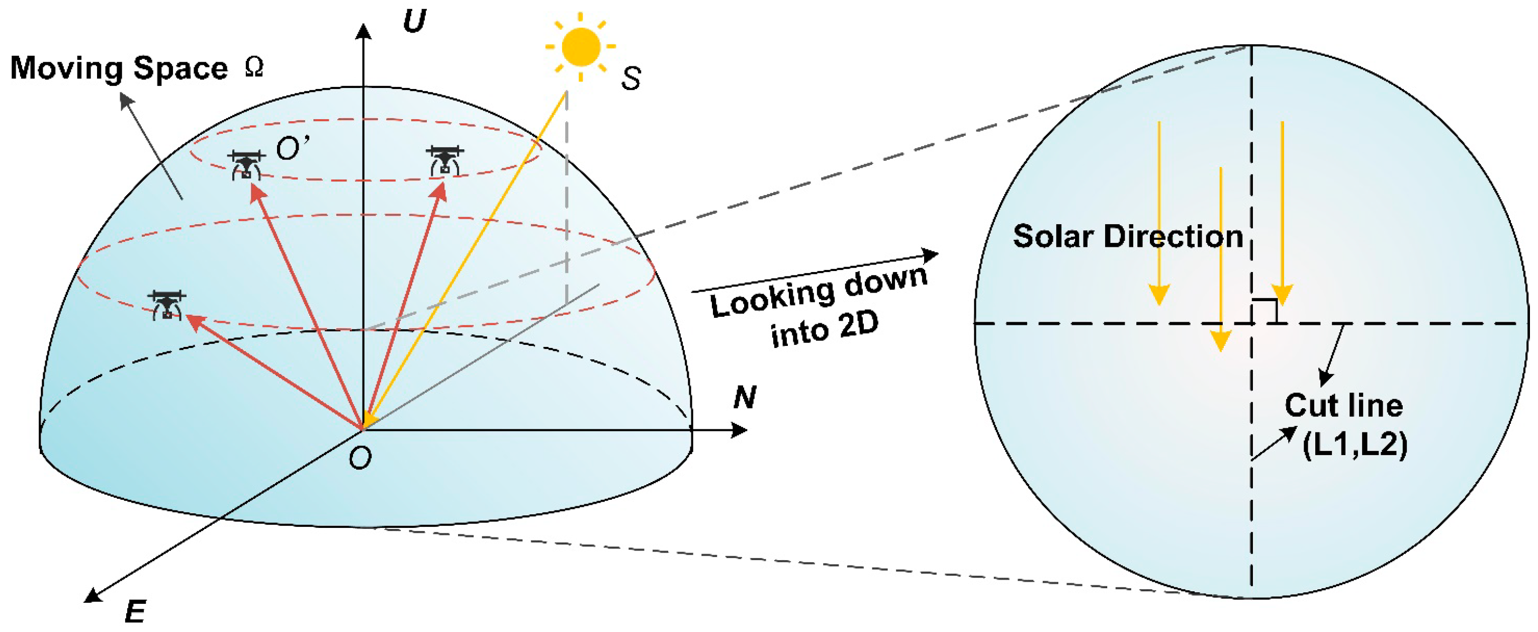
The BRDF-based solar background noise model can flexibly adapt to various changes in the optical path. The position changes of the sun and the laser during the actual measurement process are shown in Figure 4. The position of the sun is marked as point S, and it does not deviate significantly in a short period. Sunlight propagates along the direction of SO, radiates outward at the measurement point O, and is finally received by the laser at position O′. Therefore, for the propagation optical path SOO′, the directions of the sun’s position and the laser’s position can be denoted as OS and OO′, respectively. Under elliptical orbit scanning, the receiving direction of the laser constantly changes. Ideally, all possible positions and receiving directions of the laser can be simplified and described by a hemispherical space Ω, and O′ is also a point on the spherical surface. By simply traversing the receiving directions of the laser within the entire space, the top view on the right side of Figure 4 can be obtained, which allows for a more intuitive view of all the receiving directions. The cross-section line on the right side of Figure 4 is used to better compare the model differences at different receiving positions.

As can be seen from Equation (9), the position of the sun can be represented by the solar zenith angle and the solar azimuth angle. Different combinations of solar zenith angles and solar azimuth angles will have varying degrees of influence on the model results.

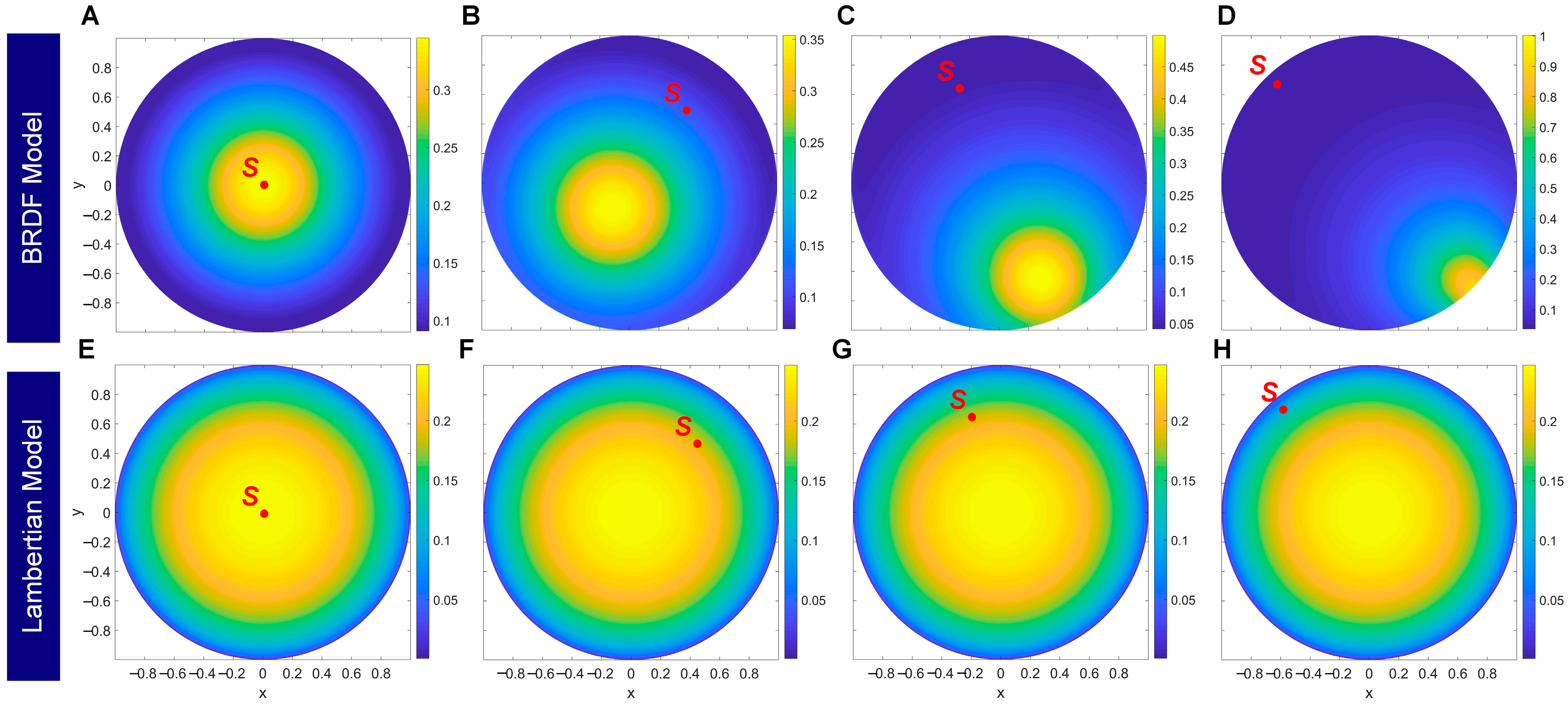
Figure 5A illustrates the spatial distribution characteristics of the noise rate calculated by the BNR-B model under different solar azimuth angles. In the experiment, the solar zenith angle was fixed at 20°, and the solar azimuth angle was sampled in all circumferential directions (from 0° to 360°) at intervals of 24°. The color in the figure is mapped to the intensity of the noise rate, and the X-Y coordinates represent the projection components of the laser receiving direction in the hemispherical coordinate system. The results show that the change in the solar azimuth angle only leads to the rigid rotation of the noise distribution pattern, while the numerical magnitude and the distribution morphology are exactly the same, verifying the rotational symmetry of the model in the horizontal plane. This characteristic indicates that the calculation results of any azimuth can be mapped to the reference azimuth (such as 0°) through a rotation transformation, and the model itself is not substantially affected by the change in the azimuth angle.

To quantify the coupling effect of the azimuth angle and the zenith angle, as shown in Figure 4, two orthogonal cross-section lines were extracted: the main-plane cross-section line L1, consistent with the solar azimuth; and the orthogonal-plane cross-section line L2, perpendicular to it. Figure 5C shows the analysis results of the cross-section lines when the solar zenith angle is 20° and the azimuth angles are 0°, 24°, 48°, and 72°. The key findings are as follows. (1) Independence of the azimuth angle: When the solar azimuth is used as a fixed reference system, the results of different azimuth angles in the L1 and L2 cross-section lines completely coincide, confirming that the change in the azimuth angle only changes the observation perspective, rather than the numerical distribution of the noise field. (2) Spatial heterogeneity: Although the noise field is generally rotationally symmetric, the significant differences between the L1 and L2 cross-section lines reveal the non-uniformity of the hemispherical reflection field. This heterogeneity stems from the directional sensitivity of the BRDF model to the incident receiving geometry.

During dynamic flight, the real-time changes in the relative position between the laser receiving direction and the sun (such as the deflection of the flight trajectory) will break the theoretical assumption of rotational symmetry. For example, even if the position of the sun is fixed, attitude disturbance or heading adjustment of the UAV platform will still change the spatial coupling pattern of the noise rate. Therefore, optimizing the design of the flight trajectory to avoid high-noise coupling areas is the key to improving the robustness of the system.

As shown in Figure 5B, the BNR-B (Background Noise Rate based on BRDF) model was evaluated under different solar zenith angles (from 0° to 90°) with the solar azimuth angle fixed at 180°. Since the model is still dominated by specular reflection, changes in the zenith angle directly adjust the incident geometry of solar noise photons, resulting in significant changes in the noise distribution pattern. When the zenith angle is small (the sun is close to the zenith), the noise rate exhibits approximately concentric circular symmetry. As the zenith angle increases (the sun approaches the horizon), the incident angle decreases, and the energy concentrates near the specular reflection direction.

Two orthogonal cross-sections were extracted from the hemispherical noise field, namely, the L1 solar principal plane and the L2 orthogonal plane, as shown in Figure 5D. The main observations are as follows: For the L1 cross-section (the principal plane), as the zenith angle increases, the peak position moves outward, which is consistent with the specular reflection geometry. At high zenith angles (>48°), except for some outliers, most of the noise rates drop to a low-intensity stable state, which reflects that the directional sensitivity is suppressed under grazing illumination conditions. For the L2 cross-section (the orthogonal plane), the peak position remains stable under different zenith angles, but the peak magnitude drops sharply from 28.64 kHz (at a zenith angle of 0°) to 4.60 kHz (at a zenith angle of 72°), indicating that the off-specular scattering decreases under oblique incidence.

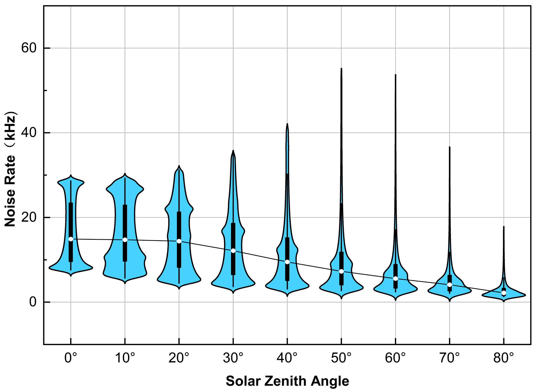
To further analyze the impact of the zenith angle on the noise rate distribution, the violin plots in Figure 6 statistically quantify the dependence of the noise rate on the zenith angle across the entire hemispherical field (zenith angles from 0° to 80°). The results show the following: (1) Affected by the weakening of the specular reflection intensity, the median noise rate (black curve) continuously decreases as the zenith angle increases. It is fitted according to the Gaussian formula as $f=15.05\ast exp\left(-{\left({\displaystyle \frac{{\theta }_s-4.192}{55.28}}\right)}^2\right)$ (${\theta }_s$ = zenith angle); $R^2=0.9959$. (2) As the zenith angle increases, the noise rates concentrate within a narrower range (the interquartile range is reduced by 68%), and the long tails indicate the existence of residual specular reflection hotspots. (3) When the zenith angle is greater than 60°, the spatial heterogeneity decreases, indicating the emergence of a quasi-uniform noise field, in which the noise levels in most directions are similar. This also means that the zenith angle determines the trade-off between noise intensity and directional uniformity. At low zenith angles (the sun is close to the zenith), high-intensity noise concentrates in the specular reflection region, which requires trajectory planning to avoid critical angles. At high zenith angles (the sun is close to the horizon), the uniform low-intensity noise simplifies the system calibration process, but it requires higher detector sensitivity.

These research results emphasize the importance of understanding the solar geometry for optimizing the operation of airborne LiDAR in coastal or mountainous terrains under dynamic lighting conditions.

3.1.2. Results of the Change in Medium Properties

In addition to the spatial-position-related parameters mentioned in Section 3.1.1, the medium itself also plays a role in determining the characteristics of the reflection cross-section during the bidirectional reflection process. Different medium properties may greatly affect the intensity of forward or backward scattering. In the current model, the medium properties are mainly characterized by the Fresnel reflectance and surface roughness parameters. Fresnel reflection refers to the change in reflectance when light is incident on the object surface at different angles [24]. The reflectance used here corresponds to the case when the light is incident vertically on the medium surface. Surface roughness is generally used to describe the undulation characteristics or smoothness of the medium surface. The specific roughness is related to properties such as surface disturbances, cracks, and particle sizes.

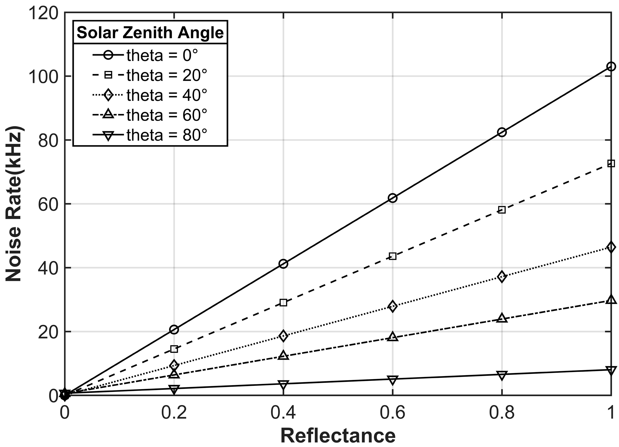
Figure 7 shows the linear relationship between the noise rate and the surface reflectance (ranging from 0 to 1) under five solar zenith angles (0°, 20°, 40°, 60°, 80°). To eliminate the directional bias and isolate the effect of reflectance, the noise rate for each configuration is represented by the hemispherical field-averaged value. As shown in the figure, all curves exhibit a linear increase with an increase in reflectance ($R^2$ > 0.99), which confirms that the reflectance is a major limiting factor of the background noise. The magnitudes of the slopes (103.00, 72.66, 46.46, 29.75, and 8.05 for the five solar zenith angles from 0° to 80°, respectively) decay exponentially with the increase in the zenith angle. The equation can be derived as $\mathrm{S}\mathrm{l}\mathrm{o}\mathrm{p}\mathrm{e}=105.9·e^{-0.02218 {\theta }_s}$ (${\theta }_s$ = zenith angle); $R²=0.9745$. This trend is consistent with the specular reflection-dominated energy redistribution; that is, smaller zenith angles enhance the sensitivity to reflectance by distributing photons over a wider angular range. However, when the zenith angle is 80°, the slope drops to 7.8% of that when the zenith angle is 0°, which reflects that the energy is severely restricted near the specular reflection direction. Therefore, under grazing illumination conditions, the change in reflectance has a minimal impact on the overall noise rate. In addition, the stable linear relationship (residual standard deviation ${\sigma }_{residual}<1.2\%$) enables the direct implementation of reflectance normalization in the noise correction process, especially applicable to nadir observations or cases with small zenith angles.

The deterministic coupling relationship between reflectance and noise simplifies the system-level error budgeting. For high-reflectance surfaces, due to the large slope of noise growth with reflectance, the dynamic range needs to be prioritized. While for low-reflectance surfaces, the detector sensitivity needs to be optimized to resolve weak signals against the background of residual noise.

Unlike the change characteristics of reflectance, the influence of roughness on the model is more random. Taking the Cook–Torrance model in this paper, the rough reflective surface of the medium can be regarded as composed of numerous micro-facets, and each micro-facet can be considered as an ideal specular reflector. Thus, during the simulation, the micro-facet distribution function describes the rough undulations of the medium surface, meaning that different medium surfaces can be characterized by different micro-facet distributions.

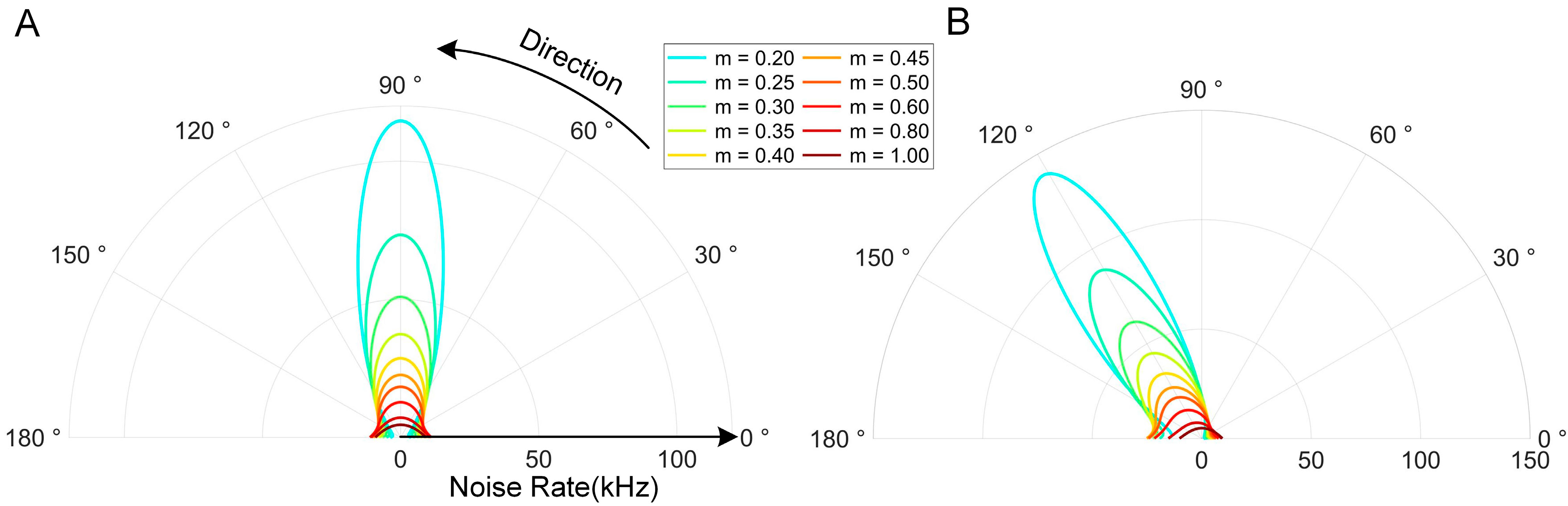
In an absolutely ideal smooth mirror environment, after a point light source is reflected the energy will only concentrate in the mirror image direction. The small-scale interface undulations described by roughness affect the radiation intensity and range of energy. When the roughness increases, the distribution of micro-surfaces in different directions will also have significant differences, which directly affects the reflection characteristics of the entire reflection cross-section. Generally speaking, only when the interface is rough will a small part of the energy be radiated to the area outside the vertical plane where the light source direction is located. To highlight the contribution of roughness to the model, an additional set of experiments is designed in this section, mainly to observe the variation law of the model within the vertical plane where the light source direction is located. As shown in Figure 4, assuming that the sun is fixed in a certain azimuth, the receivable direction of the laser is still a hemisphere composed of arbitrary directions in space. A vertical cross-section passing through the sun direction and perpendicular to the NOE plane is taken. At this time, the receivable direction of the laser changes from a hemisphere to a semi-circular arc, and the zenith angle varies within the range of 0 to 90°. Considering the angle between the receiving direction and the horizontal plane, taking the side where the sun is located as 0, the laser receiving angle can be transformed and recorded as $\tilde{\theta }$ changing from 0° to 180°. Regarding $\tilde{\theta }$ as the polar angle and calculating the model result in each direction as the polar radius, the final polar coordinate graph is shown in Figure 8.

To more intuitively observe the influence of different medium roughnesses, we selected 10 groups of roughness values within the range of 0–1 for calculation, basically covering common media such as water surfaces, sand, and land surfaces. The solar light source is placed at zenith angles of 0° and 30°, with “m” representing different roughness levels. The results are shown in Figure 8A,B. Considering that the change in the solar azimuth angle mentioned in Section 3.1.1 does not cause numerical differences, the solar azimuth angle is selected as 0° here. That is, the cross-section studied in this experiment is the plane where the solar azimuth angles of 0° and 180° are located. It can be seen from the figure that the change in the solar zenith angle does not affect the law dominated by specular reflection; that is, the energy mainly concentrates near the mirror image direction. As the solar zenith angle moves, the direction of the model result also changes accordingly. It is worth noting that this directivity is greatly weakened after the roughness exceeds a certain level. The roughness regulates the scattering direction of the micro-surfaces through the normal distribution function (NDF). When the roughness increases from 0 (specular surface) to 1 (diffuse surface), the energy is dispersed from the specular direction to a wider angular range, resulting in a decrease in the spatial heterogeneity of the noise field. Taking Figure 8A as an example, as the roughness increases, the influence of the micro-surfaces parallel to the medium plane on the distribution function gradually decreases, and more energy is radiated and dispersed to a larger area outside the vertical plane. So, intuitively, the model result seems to contract inward in a concentric structure. However, it can actually be seen that this contraction law will change to outward expansion when the laser zenith angle exceeds 84 degrees. This is because under the current model assumptions, the model result is determined by multiple parameters, especially the parameter term in the denominator related to the angle between the laser receiving direction and the normal direction. When the laser zenith angle is large, this angle is close to 90 degrees, and its cosine value is close to 0, which leads to a certain tendency for the model result to extend outward when the laser zenith angle is large. But obviously, this belongs to the internal characteristics of the model itself and does not affect the overall regular results. In Figure 8B, when the position of the sun is at the marked position of 60 degrees, the energy is mainly concentrated near the mirror image direction of 120 degrees, and the peak direction is 120 degrees. This also indicates that significant instantaneous high-intensity noise will be generated when the receiving direction of the laser coincides with the reflection direction of the sunlight. For example, when the roughness is at a relatively small value of 0.2, the noise rate can reach up to 142 kHz. It is worth noting that in an absolutely ideal situation, all the energy should be radiated in the form of forward scattering. However, due to the increase in roughness, while the overall result contracts inward, the center of gravity of scattering also shifts, manifested as a gradual weakening of forward scattering and a gradual strengthening of backward scattering. This means that under the dominance of roughness, completely different scattering characteristics can be obtained, which is also an important influencing factor in the model.

In conclusion, the background noise model established based on the BRDF reveals that the solar zenith angle dominates the noise intensity, while medium properties such as roughness regulate the scattering directionality. It provides interpretable results that conform to objective real-world laws for different scenarios, comprehensively helping us understand the action process of solar background noise. At the same time, the model is highly sensitive to parameter changes, which means it can cover most operation scenarios. However, its practical application still needs to be further verified in the future.

3.2. Experimental Results and Analysis on Jiajing Island

3.2.1. Results of Periodic Scanning

As described in Section 2.1, the experimental data cover various land-cover types such as vegetation, beaches, and water bodies (Figure 1D). Due to the data incompleteness and mixing effects in the beach and vegetation areas, this section selects a spatially continuous and homogeneous water-body area as the analysis object. Based on the method described in Section 2.3, statistical analysis of the noise rate was carried out on two typical sets of water-body data (Figure 9A,E). The results show that the measured noise rate (red curve) exhibits significant periodic fluctuations, which is in sharp contrast to the flat water-body terrain (black scatter points). The average measured noise rates of the two sets of data are 55.72 kHz and 63.48 kHz (Δ = 12%), but the fluctuations within a single set of data are intense. The standard deviations are 12.59 kHz and 10.77 kHz, and the peak-to-peak difference reaches 42.93 kHz, accounting for 68% of the average value. Under the conditions of a fixed solar position (within a 1-s period) and a homogeneous water-body medium, the periodic fluctuations of the noise rate can be attributed to the elliptical scanning mode. In this mode, the scanning period is 0.1 s, corresponding to a frequency of 10 Hz, which triggers the dynamic change in the laser receiving direction.

To verify the model, the theoretical noise rate (black curve) was compared with the measured results (red curve) (Figure 9B,F). It can be intuitively observed that the two are highly consistent in trend and magnitude. Since the measured laser has a periodic scanning characteristic, the periodicity of the measurement results is also consistent with its rotation speed of 10 r/s; that is, the rotation frequency is 10 Hz. Therefore, with the help of frequency-domain analysis, the spectral consistency and phase coherence between the two can be further quantified and revealed. As can be seen from Figure 9C,G, both the theoretical and measured values exhibit significant energy peaks at 10 Hz, confirming the noise modulation mechanism dominated by the scanning period. In the phase diagrams (Figure 9D,H) reflecting the time correlation, the phase differences corresponding to the 10 Hz components are 0.06 rad and −0.03 rad, respectively, indicating that there is almost no time deviation in the main 10 Hz components of the two groups of data. The model accurately captures the time-series characteristics of direction-dependent noise. It can be seen from this that the BNR-B noise model constructed in this study successfully replicates the periodic fluctuations of the noise rate caused by the dynamic coupling of the laser–sun geometry (the relative phase error < 2%). This demonstrates its ability to characterize direction-sensitive noise under complex optical path conditions, providing a theoretical tool for the real-time noise correction of airborne single-photon LiDAR.

3.2.2. Results with Fixed Azimuth

In order to eliminate the influence of the periodic changes of the elliptical scanning on the analysis of the measured noise rate, we selected data from the same azimuth but with different scanning periods at the same time interval for statistical analysis. We selected multiple groups of sample points from different land-cover types such as vegetation, beach, and water body to statistically analyze the measured noise rate, and analyzed the numerical values of each group of samples. Some of the results are shown in Figure 10. In this figure, the red line represents the noise rate data of the beach, the green line represents the noise rate data of the vegetation, and the blue line represents the noise rate data of the water body. Through visual interpretation, it can be clearly seen that the noise rate of the beach is higher than that of the vegetation, and the noise rate of the vegetation is higher than that of the water body. This should be related to the parameter of reflectance discussed previously. By referring to existing research, the empirical reflectance of relevant media can be obtained to support the practical application of the model [25]. Existing research shows that near the 532 nm wavelength receivable by the laser, the reflectance of the beach > the reflectance of the vegetation > the reflectance of the water body. The current pattern of the noise rate is consistent with the previously simulated rule that the greater the surface reflectance, the greater the noise rate. In addition, it can be seen that the measured noise rate of the beach fluctuates greatly, followed by that of the vegetation, and the water body has the smallest fluctuation. To clarify the conclusion obtained from the visual interpretation, we carried out numerical statistical analysis on the data, and the results are shown in

Table 1. Analysis of the measured noise rate values of different ground objects in the same azimuth.

Surface Feature	Mean (kHz)	Standard Deviation (kHz)	Coefficient of Variation
Water	46.70	2.13	4.56%
Vegetation	82.55	6.32	7.66%
Land	582.12	9.05	1.55%

.

As can be seen from Table 1, the measured noise rate of the land (beach) is the largest, with an average value reaching 582.12 kHz. This is followed by the measured noise rate of the vegetation, and the smallest is the noise rate of the water body, with an average value of only 46.7 kHz. Among them, the coefficient of variation of the vegetation is the largest, which means that the noise rate of the vegetation is the most unstable. This is because the types of vegetation and the shapes of the leaves scanned within a certain period of time may be different, resulting in differences in the noise rate results. The coefficient of variation of the beach is the smallest, because the beach, scanned within a short period of time, does not change much. And changes in the water body may be related to water surface fluctuations caused by the wind and waves.

4. Discussion

4.1. Comparative Reflection in the BRDF Model and the Lambertian Model

To evaluate the directional sensitivity of the noise rate model constructed based on the bidirectional reflectance distribution function (BRDF), we conducted controlled simulation experiments on the BRDF model and the Lambertian model under the same geometric configuration. When the LiDAR, S, was directly above the nadir reflection point (as shown in Figure 11A,E), both models showed a trend of the noise rate decreasing as the solar zenith angle increased. However, there were fundamental differences in their attenuation patterns. The Lambertian model follows an attenuation rule related to the cosine. Due to its assumption of isotropic scattering, the noise rate remains at a relatively high level over a wide range of zenith angles. In contrast, the BRDF model exhibits an attenuation characteristic dominated by specular reflection. As the energy concentrates near the reflection direction, the noise rate drops rapidly. This difference fully highlights the unique ability of the BRDF model to analyze the directional redistribution of energy, which is a key characteristic lacking in the Lambertian approximation model.

However, in actual scanning situations, when the LiDAR, S, deviates from the nadir (see Figure 11B–D for the BRDF model and Figure 11F–H for the Lambertian model), the performances of the two models are significantly different. The noise rate distribution obtained by the BRDF model is dynamically adjusted according to the changes in the geometric relationship between the LiDAR and the sun, generating a unique pattern for each receiver position. This responsiveness stems from the bidirectional reflectance formula, which clearly demonstrates the angular dependence. However, the noise rate distribution obtained by the Lambertian model does not change with the change in the LiDAR’s position. It always presents a symmetric concentric circle distribution, which fully reflects its insensitivity to direction. Since this model cannot capture the geometric modulation effect, it is not suitable for dynamic airborne application scenarios.

To systematically evaluate the directional resolution ability of the BRDF model, the same coastal flight data were selected to perform noise rate inversion using both the BRDF and Lambertian models, and a quantitative comparison was made with the measured statistical results. The specific situation is shown in Figure 12.

It can be clearly seen from the figure that the noise rate calculated based on the BRDF model is more consistent with the variation in the measured data. The BRDF model accurately reproduces the dynamic fluctuation characteristics of the measured noise rate. The RMSE of its first-order difference is 6.61 kHz, which is significantly better than the 9.26 kHz of the Lambertian model, with an accuracy improvement of 28.6%. This model can significantly reflect the influence of the laser direction on the noise rate result, which fully demonstrates that the background noise model based on BRDF has stronger adaptability and can better cope with various orbital inclination situations. With this excellent adaptability, the model can provide more accurate guidance for measurement work and effectively reduce the adverse impact of noise on data quality.

In coastal environments, these advantages of the BRDF model are particularly prominent. Due to the strong specular reflection component of the water surface, the noise situation is relatively complex. However, by virtue of the directional resolution based on micro-facets, the BRDF model successfully overcomes the problem of directionality and achieves a higher degree of consistency with the variation law of the measured noise rate, enabling it to more accurately reflect the actual noise situation.

4.2. Discussion and Analysis of Abnormal Samples in the Model

During the model validation process, we noticed two types of abnormal samples that deviated significantly from the theoretical predictions. The discovery of these two types of abnormal samples provides crucial clues for us to deeply understand the limitations of the model in practical applications.

The first type of abnormal phenomenon occurs in the shallow-water transition zone (as shown in Figure 13A). The measured noise rate gradually increases with the increase in the exposure degree of the bottom sediment, while the theoretical value remains constant because the reflectivity is not dynamically corrected. In order to explore the reasons behind this abnormal phenomenon, we carried out a detailed spatio-temporal correlation analysis (as shown in Figure 13B–D). The analysis results show that the water depth in this area gradually transitions from 5.2 m to the exposed-land state. As the water depth decreases, the bottom reflectivity increases the effective reflectivity through the water surface–bottom sediment coupling effect, resulting in an increase in the noise rate. However, since our model does not dynamically correct the reflectivity parameter and the theoretical calculation is still based on the initial assumption of the water-surface reflectivity, there is a disconnection between the predicted value and the measured trend. This case clearly reveals the potential influence of the bottom-sediment reflection coupling effect in noise modeling in the shallow-water area. To improve the adaptability of the model in this area, future research needs to introduce a joint inversion mechanism of water depth and reflectivity, jointly invert the water depth and the optical properties of the bottom sediment, and construct a dynamic reflectivity correction term to more accurately reflect the actual situation.

The second type of anomaly occurred in the deep-water stable zone (as shown in Figure 14A). In this area, both the theoretical and measured noise rates showed a downward trend (as shown in Figure 14B), decreasing by approximately 22% and 48%, respectively, which contradicts the assumption of medium stability. To uncover the mystery behind this anomaly, we integrated the analysis of the UAV’s attitude data (as shown in Figure 14C).

The analysis of the attitude data shows that during the period when the noise rate decreases, the pitch angle of the unmanned aerial vehicle changes from −3° to +3°. In order to analyze the impact of attitude changes on the noise results, we carried out a simulation experiment, as shown in Figure 14D. The results show that when the pitch angle changes from −3° to +3°, the receiving direction deviates from the main lobe of specular reflection, and the average value of the scanned noise rate decreases from 79.30 kHz to 51.50 kHz. Specifically, a negative pitch angle makes the receiving trajectory closer to the peak area of specular reflection, which is the peak area of the theoretical noise rate; while a positive pitch angle causes the receiving direction to deviate from the high-noise coupling area. This geometric deviation reduces the measured noise rate by 71.3 kHz, thus verifying the asymmetric modulation effect of attitude disturbance on the noise field. Due to the measurement error of up to 0.025° in the IMU of the selected laser, a deviation of 0.025° was added for analysis during the simulation experiment to exclude the influence of measurement errors. Through visual interpretation, it can be seen that the scanning path within the noise field when the attitude angle is 3° roughly coincides with that when it is 3.025°. After quantitative analysis, the average noise rates of the two are 51.50 kHz and 51.40 kHz, respectively, and the error range is within 0.2%.

Through analyzing the influence of attitude data on the noise rate, it is found that in scenarios with strong specular reflection, the stability of the flight attitude is a prerequisite for ensuring the stability of noise and data accuracy. In order to reduce the impact of attitude drift on the data, it is necessary to effectively suppress this impact through the control system.

The appearance of the above-mentioned abnormal samples reveals the complexity of the environment–geometry coupled noise mechanism. The research results show that although the noise model based on physical mechanisms can analyze the directional modulation law, in practical applications, it is still necessary to integrate multi-source observational data, such as water depth, attitude, and substrate information, to construct an adaptive correction framework to cope with the challenges of the dynamic heterogeneity of coastal environments. In this way, we can improve the model’s adaptability and prediction accuracy, and provide more reliable support for research and applications in related fields.

5. Conclusions and Future Perspectives

This study addresses the challenge of solar background noise modeling for unmanned aerial vehicle (UAV)-borne photon-counting LiDAR in island-reef terrain mapping and proposes a dynamic noise model (BNR-B) based on the bidirectional reflectance distribution function (BRDF), achieving a series of innovative results.

(1) Innovative Coupling of BRDF and Dynamic Light Path

A bidirectional reflectance distribution function (BRDF) model was introduced into dynamic optical path noise modeling for the first time, breaking through the isotropic assumption of traditional Lambertian reflection. By fusing the attitude data of the unmanned aerial vehicle (UAV) and the Global Navigation Satellite System (GNSS) data in real time, the geometric relationship between the sun and the receiver was dynamically corrected, solving the problem of noise modulation caused by anisotropic reflection (such as specular reflection from water surfaces and scattering from rough substrates) in coastal environments. The experiments show that the BNR-B model is highly consistent with the measured data in scenarios with complex scanning angles. Compared with traditional models, the root mean square error (RMSE) decreased from 9.26 kHz to 6.61 kHz, with an accuracy improvement of 28.6%, and the relative phase error in the frequency domain was less than 2%. This significantly enhances the ability to analyze the spatiotemporal evolution mechanism of the noise field in dynamic environments.

(2) Systematic Revelation of the Multi-Parameter Coupling Mechanism

The dynamic coupling effects of solar geometry (azimuth/zenith angle), medium properties (reflectivity, roughness), and the light path were quantified. There is a linear positive correlation between the noise rate and the medium reflectivity (R² > 0.99), and the $\mathrm{S}\mathrm{l}\mathrm{o}\mathrm{p}\mathrm{e}=105.9·e^{-0.02218 {\theta }_s}$ (${\theta }_s$ = zenith angle); $R²=0.9745$. For every 0.1 increase in reflectivity, the maximum increase in noise intensity can reach 103.0 kHz (at a zenith angle of 0°); as the zenith angle increases from 0° to 80°, the noise rate gradually converges within a narrower range, and the interquartile range is reduced by 86%; the median of the noise rate satisfies $f=15.05\ast exp\left(-{\left({\displaystyle \frac{{\theta }_s-4.192}{55.28}}\right)}^2\right)$ (${\theta }_s$=zenith angle); $R²=0.9959$. Extreme solar zenith angles (>80°) make the spatial distribution of noise more uniform, and the intensity decays to a relatively low level (4.60 kHz), providing a theoretical basis for flight trajectory optimization; roughness regulates the scattering directionality through the micro-facet distribution function. An increase in roughness reduces the spatial heterogeneity of the noise field, revealing the dominant role of the medium’s micro-structure in noise propagation.

(3) Tracing Abnormal Noise and Expanding the Model Boundaries

Two types of abnormal noise sources were discovered for the first time: the coupling reflection of bottom sediments and water surfaces in shallow water areas and the pitch-angle drift of UAVs. The noise fluctuation reached 71.3 kHz. The geometric–environment coupling mechanisms in abnormal scenarios were clarified, pointing out the direction for dynamic model correction (such as joint inversion of reflectivity and attitude stability control).

Subsequent research will focus on the following key points:

(1) Multi-physical field coupling modeling: The current model mainly focuses on the influence of solar radiation. In the future, factors such as atmospheric turbulence and aerosol scattering can be incorporated. The atmospheric radiation transmission model can be coupled to dynamically correct the atmospheric transmittance, and a noise prediction system with multi-physical field coupling can be constructed.

(2) Model optimization: In view of the sudden increase in prediction errors of the existing model in the land–water junction area (within ±5 km from the coastline), a dynamic inversion algorithm for reflectivity parameters that integrates microwave remote sensing data could be developed. Considering the complex calculations and high requirements for computing resources of the existing model, subsequent research could reduce the computational cost through parallel computing architectures and algorithm simplification.

(3) Improving the universality of the model: Currently, the model has only been applied and experimentally verified on Jiajing Island and does not cover verification scenarios with extreme solar positions. To enhance the universality of the model, extensive experimental verification work with different solar positions at different times needs to be carried out in more coastal zone areas of different types. By selecting experimental areas with different climatic conditions, geological structures, and ecological environments, more diverse data can be collected to optimize and improve the model, ensuring that the model can adapt to various complex measurement scenarios and has better universality.

References

1. Yu, Y.; Wang, Z.; Li, H.; Yu, C.; Chen, C.; Wang, X.; Li, X.; Xue, B.; Pan, X.; Zhuang, Q.; et al. High-precision 3D imaging of underwater coaxial scanning photon counting Lidar based on spatiotemporal correlation. Measurement 2023, 219, 113248. [Google Scholar] [CrossRef]
2. Luan, K.; Zhao, X.; Kong, W.; Chen, T.; Xie, H.; Liu, X.; Wang, F. A Novel Ray Tracing Approach for Bathymetry Using UAV Based Dual-polarization Photon-counting LiDAR. IEEE J. Sel. Top. Appl. Earth Obs. Remote Sens. 2024, 17, 20284–20303. [Google Scholar] [CrossRef]
3. Zhang, H.; Wang, L.; Zhao, Y.; Cao, J.; Xu, M. Application of airborne LiDAR measurements to the topographic survey of the tidal flats of the Northern Jiangsu radial sand ridges in the Southern Yellow Sea. Front. Mar. Sci. 2022, 9, 871156. [Google Scholar] [CrossRef]
4. Jiao, C.; He, Y.; Hu, S.; Liu, H.; Chen, W.; Zhang, W. Effects of solar radiation on the performance of long-distance atmosphere-ocean laser communication links. Opt. Commun. 2025, 574, 131051. [Google Scholar] [CrossRef]
5. Oren, M.; Nayar, S.K. Generalization of the Lambertian model and implications for machine vision. Int. J. Comput. Vis. 1995, 14, 227–251. [Google Scholar] [CrossRef]
6. Peng, Z.; Wang, H.; She, X.; Xue, R.; Kong, W.; Huang, G. Marine remote target signal extraction based on 128 line-array single photon LiDAR. Infrared Phys. Technol. 2024, 143, 105592. [Google Scholar] [CrossRef]
7. Degnan, J.J. Photon-counting multikilohertz microlaser altimeters for airborne and spaceborne topographic measurements. J. Geodyn. 2002, 34, 503–549. [Google Scholar] [CrossRef]
8. Zhang, Z.; Ma, Y.; Xu, N.; Li, S.; Sun, J.; Wang, X.H. Theoretical background noise rate over water surface for a photon-counting lidar and its application in land and sea cover classification. Opt. Express 2019, 27, A1490–A1505. [Google Scholar] [CrossRef]
9. Zhang, W.; Xu, N.; Ma, Y.; Yang, B.; Zhang, Z.; Wang, X.H.; Li, S. A maximum bathymetric depth model to simulate satellite photon-counting lidar performance. ISPRS J. Photogramm. Remote Sens. 2021, 174, 182–197. [Google Scholar] [CrossRef]
10. Yang, J.; Zheng, H.; Ma, Y.; Zhao, P.; Zhou, H.; Li, S.; Wang, X.H. Background noise model of spaceborne photon-counting lidars over oceans and aerosol optical depth retrieval from ICESat-2 noise data. Remote Sens. Environ. 2023, 299, 113858. [Google Scholar] [CrossRef]
11. Zheng, H.; Yang, J.; Ma, Y.; Ma, Y.; Zhou, H.; Wang, X.H.; Li, S. Derived reflectance over open oceans using ICESat-2 background noise and auxiliary data. IEEE Trans. Geosci. Remote Sens. 2023, 61, 5703112. [Google Scholar] [CrossRef]
12. Zhang, Z.; Xu, N.; Ma, Y.; Liu, X.; Zhang, W.; Li, S. Land and snow-covered area classification method based on the background noise for satellite photon-counting laser altimeters. Opt. Express 2020, 28, 16030–16044. [Google Scholar] [CrossRef] [PubMed]
13. Wang, Y.; Yang, X.; Wang, C. Vegetation and land classification method based on the background noise rate of a photon-counting LiDAR. Opt. Express 2022, 30, 14121–14133. [Google Scholar] [CrossRef] [PubMed]
14. Chen, X.; Kong, W.; Chen, T.; Huang, G.; Shu, R. Fiber-laser-pumped green laser for photon-counting bathymetric Lidar on UAV platform. In Proceedings of the Seventh Symposium on Novel Photoelectronic Detection Technology and Applications, Kunming, China, 5–7 November 2020; SPIE: Nuremberg, Germany, 2021; Volume 11763, pp. 895–902. [Google Scholar]
15. Yue, X.; Teng, F.; Lin, Y.; Hong, W. Target anisotropic scattering deduction model using multi-aspect SAR data. ISPRS J. Photogramm. Remote Sens. 2023, 195, 153–168. [Google Scholar] [CrossRef]
16. Luan, K.F.; Zhang, K.N.; Qiu, Z.G.; Wang, J.; Wang, Z.H.; Xue, Y.; Zhu, W.D.; Ling, D.D.; Zhao, X.Y. Denoising method for light weight photon counting LiDAR based on an improved local sparse coefficient. Natl. Remote Sens. Bull. 2023, 27, 520–532. [Google Scholar] [CrossRef]
17. Chang, B.; Xiong, H.; Li, Y.; Pan, D.; Cui, X.; Zhang, W. ALCSF: An adaptive and anti-noise filtering method for extracting ground and top of canopy from ICESat-2 LiDAR data along single tracks. ISPRS J. Photogramm. Remote Sens. 2024, 215, 80–98. [Google Scholar] [CrossRef]
18. Zhao, Y.; Tian, Y.; Ye, J.; Wu, Y.; Zhao, Z.; Chi, Z.; Tian, T.; Yao, H.; Hu, J.; Chen, Y.; et al. Universal dissipative dynamics in strongly correlated quantum gases. Nat. Phys. 2025, 21, 530–535. [Google Scholar] [CrossRef]
19. Cook, R.L.; Torrance, K.E. A reflectance model for computer graphics. ACM Trans. Graph. (ToG) 1982, 1, 7–24. [Google Scholar] [CrossRef]
20. Stitch, M.L. Laser rangefinding. In Laser Handbook; North-Holland Publishing: Amsterdam, The Netherlands, 1972; Volume 2, pp. 1745–1784. [Google Scholar]
21. Degnan, J.; McGarry, J.; Zagwodzki, T.; Dabney, P.; Geiger, J.; Chabot, R.; Steggerda, C.; Marzouk, J.; Chu, A. Design and performance of an airborne multikilohertz photon-counting microlaser altimeter. Int. Arch. Photogramm. Remote Sens. Spat. Inf. Sci. 2001, 34, 9–16. [Google Scholar]
22. Reda, I.; Andreas, A. Solar position algorithm for solar radiation applications. Sol. Energy 2004, 76, 577–589. [Google Scholar] [CrossRef]
23. Shumway, R.H.; Stoffer, D.S. Spectral Analysis and Filtering. In Time Series Analysis and Its Applications; Springer Texts in Statistics; Springer: Cham, Switzerland, 2025. [Google Scholar]
24. Querry, M.R. Direct solution of the generalized Fresnel reflectance equations. J. Opt. Soc. Am. 1969, 59, 876–877. [Google Scholar] [CrossRef]
25. Lillesand, T.; Kiefer, R.W.; Chipman, J. Remote Sensing and Image Interpretation; John Wiley & Sons: Hoboken, NJ, USA, 2015; pp. 12–25. [Google Scholar]
Figure 1. (A,B) Schematic diagram of the experimental area. (The area within the red frame in the figure is the selected data area). (C) Schematic diagram of point cloud data. (D) Schematic diagram of the measured strip data after denoising. (The dashed lines represent the feature types of each data respectively).
Remotesensing 17 01708 g001
Figure 2. (A) Schematic diagram of laser scanning. (B) Schematic diagram of the positional relationship between the laser and the sun. (The blue dotted line represents the trace points).
Remotesensing 17 01708 g002
Figure 3. Schematic diagram of the statistical method used to determine the measured noise rate.
Remotesensing 17 01708 g003
Figure 4. The half-space of the receiving direction vector of the laser and its top view. (The black aircraft is the position of the laser).
Remotesensing 17 01708 g004
Figure 5. (A) Distribution diagram of the noise field at different solar azimuth angles. (B) Distribution diagram of the noise field at different solar zenith angles. (C) Comparison diagram of the results of the transverse lines of the noise field under different solar azimuth angles. (D) Comparison diagram of the results of the transverse lines of the noise field under different solar zenith angles.
Remotesensing 17 01708 g005
Figure 6. Violin plot of the distribution of the noise field at different solar zenith angles.
Remotesensing 17 01708 g006
Figure 7. Result graph of the noise rate for different reflectance and solar zenith angles.
Remotesensing 17 01708 g007
Figure 8. (A) result diagram of the noise under a solar zenith angle of 0 degrees with different roughness. (B) result diagram of the noise under a solar zenith angle of 30 degrees with different roughness.
Remotesensing 17 01708 g008
Figure 9. (A) Result diagram of the point cloud of data 1 and the measured noise rate. (B) Comparison diagram between the measured and theoretical noise rates of data 1. (C) Frequency–amplitude diagram of the measured and theoretical noise rates of data 1. (D) Phase difference diagram of the measured and theoretical noise rates of data 1. (E) Result diagram of the point cloud of data 2 and the measured noise rate. (F) Comparison diagram between the measured and theoretical noise rates of data 2. (G) Frequency–amplitude diagram of the measured and theoretical noise rates of data 2. (H) Phase difference diagram of the measured and theoretical noise rates of data 2.
Remotesensing 17 01708 g009
Figure 10. Result diagram of the measured noise rates for different types of ground objects.
Remotesensing 17 01708 g010
Figure 11. (AD) Result diagram of the noise rates at different solar positions when the laser is at point S calculated by the BRDF model. (EH) Result diagram of the noise rates at different solar positions when the laser is at point S calculated by the Lambertian model.
Remotesensing 17 01708 g011
Figure 12. Comparison of the noise rates calculated by the BRDF model and the Lambertian model with the measured noise rates.
Remotesensing 17 01708 g012
Figure 13. (A) Diagram of the changes in the measured and theoretical noise rates in the water–land transition area. (B) Point cloud data diagram of the deep-water area. (C) Point cloud data diagram of the shallow-water area. (D) Point cloud data diagram of the exposed-land area.
Remotesensing 17 01708 g013
Figure 14. (A) Schematic diagram of the measured noise rate and the point cloud data. (B) Schematic diagram of the measured and theoretical noise rates. (C) Diagram of attitude changes within different time periods. (D) Schematic diagram of the scanning results in the noise field under different pitch-angle conditions.
Remotesensing 17 01708 g014