Estimation of Chlorophyll Content at Stand and Individual Tree Level by UAV Hyperspectral Combined with LiDAR

Abstract

Chlorophyll plays a significant role in evaluating vegetation health and forest carbon sink. In this study, a total of 36 characteristic variables from hyperspectral image and lidar point cloud data acquired through an unmanned aerial vehicle (UAV) platform were used to evaluate the accuracy of statistical models including multiple stepwise regression, BP neural network, BP neural network optimized by firefly algorithm, random forest, and the mixed data-driven mechanistic model PROSPECT model in estimating chlorophyll content for three different forest types in Maoershan Forest Farm of Northeast Forestry University in Heilongjiang Province, namely coniferous forest, broad-leaved forest, and coniferous–broad-leaved mixed forest. The accuracy of the models was evaluated by the coefficient of determination (R²) and root mean square error (RMSE). The results show that random forest (R² = 0.59–0.64, RMSE = 3.79–5.83 µg·cm⁻²) among all statistical models is superior to other models. The accuracy of the mechanism model was the highest (R² = 0.97, RMSE = 3.40 µg·cm⁻²). There were significant differences in chlorophyll content among different forest types. It ranged from 25.25 to 31.60 µg·cm⁻² for broad-leaved forests, which was higher than that of coniferous and broad-leaved mixed forests (13.52–23.93 µg·cm⁻²) and coniferous forests (6.40–13.71 µg·cm⁻²). In the horizontal direction, the chlorophyll content near the center of the canopy was lower than that at the edge of the canopy. In the vertical direction, there was no significant difference in chlorophyll content between different canopies of Pinus sylvestris var. mongolica, while there was a significant difference in chlorophyll content between the upper, middle, and lower canopies of Juglans mandshurica. For different tree species, the variation in chlorophyll with crown height was different.

1. Introduction

Forest is a complex functional aggregate in the ecosystem [1,2]. Chlorophyll, as a key pigment in forest vegetation, has functions such as maintaining photosynthesis and indicating environmental stress. It is an important indicator for forest ecosystem evaluation [3], and its distribution shows significant differences in space [4]. Therefore, accurately estimating the spatial distribution of forest chlorophyll content is crucial for forest ecosystem studies [5]. However, obtaining samples in the complex vertical and horizontal structures of forests is time-consuming, expensive, and destructive [6]. Remote sensing technology for chlorophyll content estimation using hyperspectral data and LiDAR overcomes the limitations of traditional field measurement [7,8,9]. The hyperspectral sensor can acquire hundreds of narrow bands with abundant spectral information. Continuous high-resolution spectral images of the study area can be obtained through the UAV platform with simple operation, flexible application, and low cost [10], which avoids the disadvantages of few satellites and low resolution in the existing hyperspectral data acquisition. This provides an important data basis for the estimation of chlorophyll content in horizontal structure. Accurate estimation of chlorophyll content in the vertical direction requires LiDAR technology, which provides forest vertical structure information. LiDAR can effectively compensate for the lack of vertical information in hyperspectral data and provide more details [11]. The fusion of hyperspectral data and LiDAR has been widely applied in forestry, including tree-species identification [12,13,14], forest type classification, forest biochemical parameter inversion [15,16,17,18], and forest pest–diseases monitoring [19,20,21].

In terms of chlorophyll content estimation, there are relatively few studies on the joint estimation of unmanned aerial vehicle hyperspectral and LiDAR data, which mainly rely on hyperspectral data. Models for chlorophyll content estimation include empirical models and physical models [22]. Liao [23] proposed a new fusion framework through deep learning. This framework realizes the complementary information of hyperspectral and radar data for mapping, thereby improving the accuracy of tree species classification. Dong [24] obtained the Digital Surface Model (DSM) and Digital Terrain Model (DTM) from airborne lidar point cloud data. Further, by taking the difference, the Normalized Digital Surface Model (nDSM) was acquired. The normalized index was calculated using high-resolution imagery, and Principal Component Analysis (PCA) was employed for denoising and dimensionality reduction. Through the fusion of PCA images and nDSM images, the Maximum Likelihood Classification (MLC) method was used for supervised classification. The overall accuracy of extracting buildings and trees was 84.00%. For example, a backward stepwise regression model was used in Shen’s study to find a significant difference in the vertical distribution of biochemical traits on the surface of Metasequoia glyptostroboides and Populus tomentosa Carr [16]. Yin used the radiation transfer model (PROSAIL) to plot the pigment distribution of Ginkgo biloba at different ages, showing significant differences [17]. Blackburn developed a method for estimating the chlorophyll concentration in artificial broadleaf and coniferous forests using an airborne imaging spectrometer and LiDAR [25]. Koetz obtained comprehensive forest canopy characteristics from the combined remote sensing signals of imaging spectroscopy and large-footprint LiDAR, enabling reliable estimation of forest chlorophyll content [26]. The empirical method is simple and easy to implement, especially in recent years, the machine learning algorithm has been well applied in the inversion of biochemical parameters. Compared with the linear model, it considers the nonlinear relationship between variables and improves the robustness of prediction. Although the physical method needs to input complex parameters, the model is not affected by time and region, and the model has good mobility, stability, and high accuracy [22,27]. 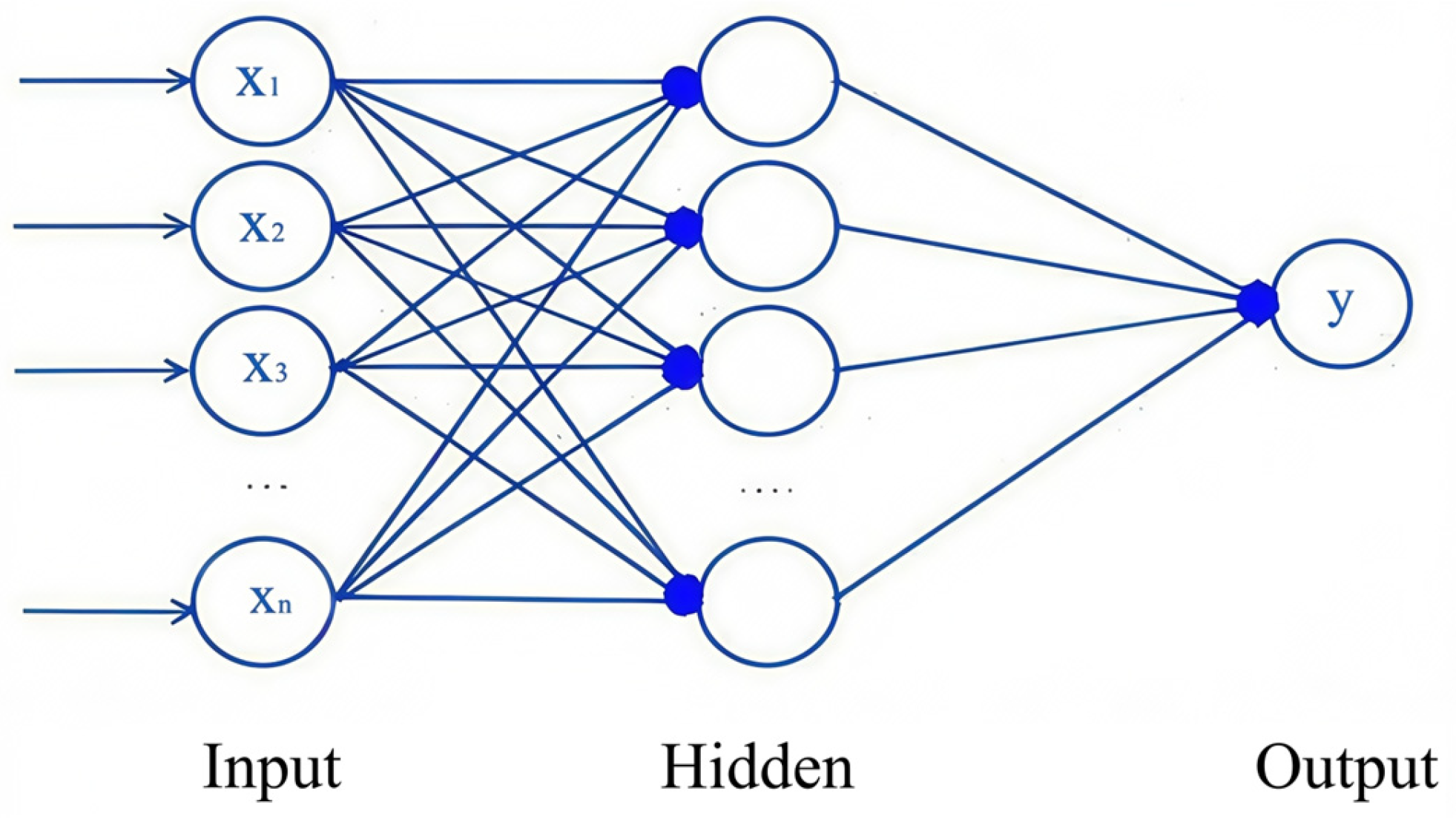There are more studies on the spatial distribution of chlorophyll in agriculture [28], while in forestry, most studies focus on the horizontal direction, and some scholars are dedicated to the analysis of the vertical spatial distribution of chlorophyll [16,17,18,29]. However, studies exploring the vertical spatial distribution of chlorophyll in different forest stands are still relatively few. Meanwhile, chlorophyll content estimation is mainly focused on the single-wood level, so there is still room for exploration in the accurate estimation of chlorophyll content at the stand level. Remote sensing monitoring of vegetation chlorophyll is mainly based on hyperspectral images, and the methods adopted mainly include statistical model methods (multiple stepwise regression, neural networks, random forests) and physical model methods (radiative transfer model method) [30,31].

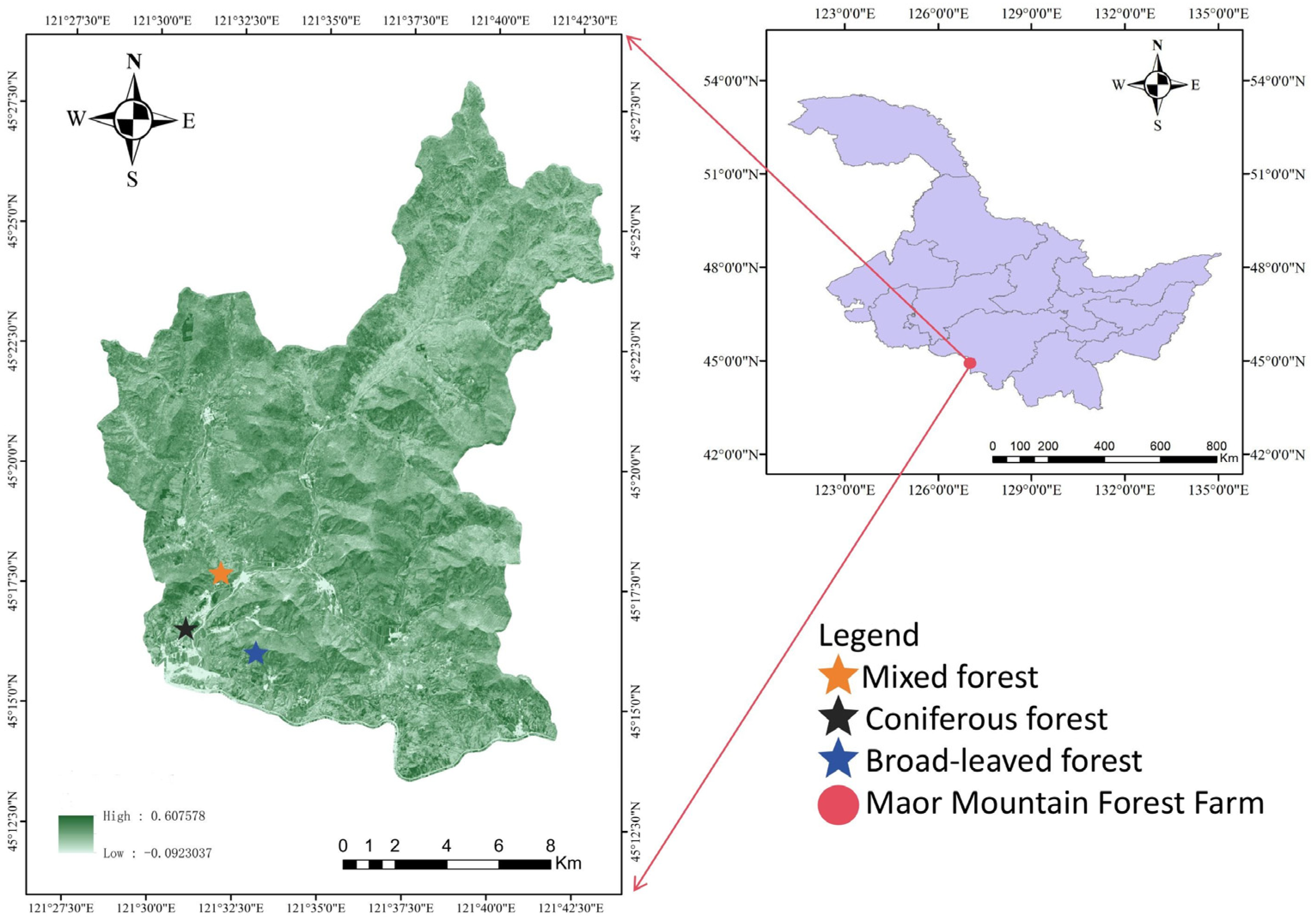
In this study, hyperspectral and LiDAR data were used to construct the three-dimensional spatial distribution of chlorophyll content among different forest types. This study explored the accuracy and differences in chlorophyll content estimation using multiple stepwise regression, random forest, BP neural network, firefly algorithm optimized BP neural network, and mechanistic modeling methods driven by a mixture of measured and simulated data. The optimal model for chlorophyll estimation was determined, and the spatial distribution pattern of chlorophyll content at the single tree and stand scale was clarified. By timely and accurately estimating the spatial distribution of chlorophyll in different forest stands and individual trees, a scientific basis is provided for effective forest management and regional carbon-neutral evaluation.

2. Materials and Methods

2.1. Study Area and Data

2.1.1. Overview of the Study Area

The research area is located in Maor Mountain Forest Farm, Shangzhi City, Heilongjiang Province (45°02′20″–45°18′16″N, 127°18′00″–127°41′06″E). The mountainous area is hilly and the terrain is high in the south and low in the north, with a slope of 5 to 25° and an altitude of 200 to 600 m. The experimental area is affected by the continental monsoon, with cold and dry winters, rainy and hot summers, and an average annual precipitation of 700 mm. The soil type is mainly dark brown soil, which is suitable for all kinds of vegetation. The main tree species in the research area include Pinus koraiensis, Fraxinus mandschuria, Larix gmelinii (Ruprecht) Kuzeneva, Juglans mandshurica, Betula platyphylla, and Ulmus pumila. As shown in Figure 1, it represents the study area.

2.1.2. Experimental Design

Three 100 m × 100 m sample plots were set up in coniferous forest, broad-leaved forest, and mixed forest in the study area, and structural parameters such as tree height, DBH, and crown width were recorded. A total of 2~3 sample trees for each species with good crown shape were selected in each plot, totaling 26 trees. The crown was divided into upper, middle, and lower layers in different directions (east, south, west, and north). For each layer, 10 leaves were collected using branch cutters in each direction, placed in a 0 °C cooling box, and returned to the laboratory for chlorophyll content measurement. Remote sensing data were obtained on 30 and 31 August 2021, which were synchronized with the collection of chlorophyll content in leaves. The UAV system M300RTK was equipped with hyperspectral imager Pika L and RIEGL mini VUX-IUAV small laser scanning system. After 10:00 on the same day, data were collected under the condition of stable lighting conditions. Pika L collected 12-bit images of 561 spectral channels at an average height of 200 m above the ground and records data in BIL format. The drone LiDAR data acquisition altitude is 80 m relative to the ground, with an average flight speed of 5.0 m·s⁻¹, an average point cloud density of 104 pts·m⁻², and a laser pulse wavelength of 905 nm. The data storage format is the standard LiDAR storage format, LAS, which includes coordinates, echo intensity, echo frequency, elevation, and other information (

Table 1. Remote sensing equipment parameters.

Parameter	Hyperspectral (Pika L)	LiDAR (RIEGL Mini VUX-IUAV)
Data of acquisition	2021-08-30–2021-08-31	2021-08-30–2021-08-31
Flight height (m)	200	80
Flight speed (m·s−1)	5.0	5.0
Side overlap (%)	30	10
Focal length (mm)	17	-
IFOV/beam divergence (mrad)	0.88~17.00 mm	1.6
Spatial resolution/footprint (cm)	10	16
FOV/maximum scan angle (°)	17.6~17.0 mm	±40
Wavelength (nm)	400~1000	905
Spectral sampling (nm)	2.1	-
Number of bands	300	1
Average point density (pts·m−2)	-	104

).

The acquired hyperspectral data are processed using the post-differencing technique for POS data in the QinertiaINS PPK post-differencing processing software. The prepared original hyperspectral images are pre-segmented for the hyperspectral data in the ENVI 5.3 software. Geometric correction of the images is carried out using Mega-Cube, and at the same time, radiometric calibration is performed using the radiometric calibration files. Subsequently, geographic registration of the images is conducted in ArcGIS based on the inter-flight image overlap rate. The registered images are mosaicked using ENVI 5.3. The mosaicked images are then used to create a hypercube in Mega-Cube. Finally, the hypercube is converted into a reflectance image.

The ground points were obtained by point cloud denoising, filtering, and classification, using Irregular Triangular Network (TIN) interpolation to obtain the Digital Elevation Model (DEM). By using point cloud thinning, the image shape and quality were ensured while improving the processing efficiency of point clouds. After thinning the point cloud, the average value of the highest point of the crown surface in each grid was calculated to establish a Digital Surface Model (DSM) with the same spatial resolution as hyperspectral data. The preprocessing of hyperspectral data included geometric correction, geographic registration, image stitching, and hypercube conversion reflectance. After the post-differential technology is used to process the data from the base station GPS and IMU records of the UAV system, the research area is cut out by hyperspectral pre-segmentation technology. As shown in Figure 2, the hyperspectral pre-segmentation was carried out using the watershed segmentation method in ENVI.

The unmanned aerial vehicle hyperspectral image and LiDAR point cloud were fused by DSM [16]. Before fusion, five ground control points were randomly selected in each grid of 10 m × 10 m to achieve the common registration of hyperspectral images and DSM to ensure the fusion accuracy. The LiDAR point cloud was divided into a matrix consistent with hyperspectral spatial resolution (0.1 m × 0.1 m), from which the highest LiDAR point in each matrix column was selected, and other points were eliminated. And then the hyperspectral reflectivity information was mapped to the highest point in each grid [16]. By fusing data, complementary information can be achieved between hyperspectral and LiDAR point cloud data to form hyperspectral point clouds.

2.1.3. Leaf Reflectance Simulated by PROSPECT Model

PROSPECT is a radiation transfer model based on Allen’s generalized “flat plate model”, which can simulate spectral reflectance and transmittance in the range of 400~2500 nm [32]. Leaf parameters, such as pigment concentration, equivalent water thickness, and dry matter content, were selected to simulate spectral reflectance and transmittance in the model.

Before applying the PROSPECT model, a sensitivity analysis of the parameters was required. Local sensitivity analysis method can be used to evaluate the influence of variables on the model under the condition of gradient change. The formula is as follows:

$$S_i={\sum }_{j=1}^n{\displaystyle \frac{|R_i\left(X+∆X\right)-R_I(X\left)\right|}{R_i\left(X\right)}}$$

(1)

where S_i represents the sensitivity of each parameter in the i-band; n is the number of times the model parameter step size changes; R_i(X) is the leaf reflectance at reference point X; and i is the number of wave bands.

2.1.4. Feature Selection

The sensitivity analysis of chlorophyll shows that the disturbance of chlorophyll is mainly manifested in visible light and near-infrared light. In the experiment, the spectra of 400~850 nm leaves were selected for Pearson correlation analysis with chlorophyll. To include more variables related to chlorophyll, logarithmic forms of spectral reflectance lgR, band spectral normalization, and spectral ratio were added. High correlation bands and band combinations were selected as candidate variables for model construction. As well, based on previous research, three edge parameters (red edge, yellow edge, and blue edge) and vegetation indices were also selected [5], such as NDVI, RENDVI, EVI, OSAVI, PRI, etc. (

Table 2. Chlorophyll-related vegetation index.

Index Name	Equation	Reference
Red-edge normalized difference vegetation index (RENDVI)	(RNIR − RRed-edge)/(RNIR + RRed-edge)	[33]
Green norm difference vegetation index (GNDVI)	(RNIR − RGreen)/(RNIR + RGreen)	[34]
Simple ratio (SR)	RNIR/RRed	[35]
Normalized green-red difference index (NGRDI)	(RGreen − RRed)/(RGreen + RRed)	[36]
Normalized difference vegetation index (NDVI)	(RNIR − RRed)/(RNIR + RRed)	[37]
Modified chlorophyll absorption reflectance index (MCARI)	[(R700 − R670) − 0.2 × (R700 − R550)] × (R700/R670)	[38]
Enhanced vegetation index (EVI)	2.5 × [(R821 − R688)/(1 + R821 + 6 × R688 − 7.5 × R461)]	[39]
Structurally insensitive pigment index (SIPI)	(R800 − R445)/(R800 + R680)	[40]
Chlorophyll absorption reflectance index (CARI)	(R700 − R670) − 0.2 × (R700 − R550)	[41]
Optimized soil-adjusted vegetation index (OSAVI)	(1 + 0.16) × (R800 − R670)/(R800 + R670 + 0.16)	[42]
Transformed chlorophyll absorption reflectance index (TCARI)	3 × [(R700 − R670) − 0.2 × (R700 − R550) × R700/R670]	[42]
TCARI/OSAVI	TCARI/OSAVI	[42]
Photochemical reflectance index (PRI)	(R531 − R570)/(R531 + R570)	[43]
Plant senescence reflectance index (PSRI)	(R678 − R500)/R750	[44]
Red edge (Dr)	The maximum value of the first derivative of the reflection spectrum in the range of 680–760 nm	[5]
Yellow edge (Dy)	The maximum value of the first derivative of the reflection spectrum in the range of 560–640 nm	[5]
Blue edge (Db)	The maximum value of the first derivative of the reflection spectrum in the range of 490–530 nm	[5]
R663	Laboratory band for chlorophyll content measurement	[5]
R645	Laboratory band for chlorophyll content measurement	[5]

), and finally, 36 variables were obtained from each stand as model candidate variables. In our study, to control spatial autocorrelation errors, we employed stratified sampling. This method helped in reducing biases related to spatial clustering. It should be noted that a limitation exists: neither random forest, BP neural network, nor physical models can account for the lack of independence among samples.

To incorporate more feature variables, the normalized difference vegetation index (NDVI) and the ratio vegetation index (RVI) of arbitrary bands were constructed. Then, a correlation analysis was conducted with the measured chlorophyll content values. According to the magnitude of the determination coefficient, five bands with high correlations were selected as candidate feature variables from different band ranges.

$$NDVI={\displaystyle \frac{(R_{\mathsf{\lambda }\mathrm{i}}-R_{\lambda j})}{R_{\mathsf{\lambda }\mathrm{i}}+R_{\lambda j}}}$$

(2)

$$RVI={\displaystyle \frac{R_{\mathsf{\lambda }\mathrm{i}}}{R_{\lambda j}}}$$

(3)

where $R_{\mathsf{\lambda }\mathrm{i}}$ and $R_{\lambda j}$ represent the reflectance at any wavelength within the range of 400–850 nm.

Meanwhile, the reflectance values at two wavelengths, R₆₆₃ and R₆₄₅, which are measured during the laboratory determination of chlorophyll content, were also incorporated into the candidate characteristic variables. The wavelength range for the near-infrared band is 780 nm to 1400 nm, and the wavelength range for the green band is 495 nm to 570 nm.

2.2. Model Construction

2.2.1. Multiple Stepwise Regression Model

The multiple linear stepwise regression model is simple to construct and widely applied. It is a commonly used method for constructing prediction models in forest pigment inversion. This model can appropriately increase or decrease n independent variables, selectively choose sensitive independent variables, eliminate redundant variables, ensure the effectiveness of variables for the model, and ultimately obtain an ideal linear regression equation [45]. In the multiple linear stepwise regression model, there are three main methods for selecting independent variables: forward selection, backward selection, and stepwise screening. The stepwise screening method combines the forward and backward selection methods. It not only endows the selected independent variables with statistical significance but also reduces the computational load. Moreover, it ensures a strong correlation between the independent and dependent variables [46]. In the process of establishing a regression equation, the multiple stepwise regression method can screen variable factors. Ju [47] used this method to invert forest biomass. Shen [48] utilized the multiple stepwise regression method to achieve the inversion of subtropical forest biomass. Li [49] also constructed an estimation model for the chlorophyll content of Phyllostachys edulis under pest stress through multiple stepwise regression analysis.

2.2.2. Random Forest Model

Random forest is a powerful integrated machine learning algorithm that can use random subsets to guide the construction of a large number of decision trees on a dataset. It has superior generalization ability and can evaluate model accuracy based on out-of-the-bag data to avoid overfitting the model [50]. The 36 variables pre-selected from each stand were sorted by importance, and variables with the importance threshold above 0.5 were selected to establish the model. In the model, the number of decision tree variables and the minimum number of decision tree nodes are taken as default values. The number of decision trees varies between 80 and 1000, with 80% of the data used for training and 20% for testing. For 80% of the data (the training set), ten-fold cross-validation was employed to tune the model parameters, and then the remaining 20% of the data were used for testing.

2.2.3. BP Neural Network Model

BP neural network consists of three layers: input layer, hidden layer, and output layer. The variables are the same as those in the random forest model. The initial number of hidden layer nodes is 2~15, and the number of neurons in the output layer is 1. By linking the inputs and outputs of the neural network in the hidden layer, the connection weight between the network connection layers is adjusted according to the actual error. And finally, reaching the input layer, the model estimation accuracy is improved. However, the BP neural network is prone to getting stuck in local minima and has problems such as slow convergence speed. Figure 3 presents the BP neural network in the form of a picture.

2.2.4. Optimization of BP Neural Network Model

To solve the problem of slow convergence speed in BP neural network, firefly algorithm is selected for model optimization, and 500 training sessions are conducted at a learning rate of 0.1. The firefly algorithm is an algorithm based on swarm intelligence. It is a meta-heuristic algorithm developed by Yang [51] in 2008 based on the behavior of fireflies using flash signals to attract other fireflies to find potential mates. Its advantage is that it can achieve automatic subdivision and is very suitable for optimizing highly nonlinear problems. Secondly, it has multimodal characteristics and faster convergence speed when dealing with multimodal problems [52]. Compared with genetic algorithms and Particle Swarm Optimization algorithms, it has certain advantages.

2.3. Accuracy Evaluation of the Model

The accuracy of the model is tested using the coefficient of determination (R²) and root mean square error (RMSE):

$$R^2=1-{\displaystyle \frac{{\sum }_{i=1}^n{(y_i-\widehat{y_i})}^2}{{\sum }_{i=1}^n{(y_i-\overline{y_i})}^2}}$$

(4)

$$RMSE=\sqrt{{\displaystyle \frac{{\sum }_{i=1}^n{(y_i-\widehat{y_i})}^2}{n}}}$$

(5)

where $y_i$ is the measured value of chlorophyll. $\widehat{y_i}$ is the estimated value of chlorophyll. $\widehat{y_i}$ is the average measurement value of the sample. i is the sample number. The larger the R², the smaller the RMSE and the higher the model estimation accuracy.

2.4. Analysis of Spatial Distribution of Chlorophyll Content at the Scale of Individual Trees

Influenced by genetic characteristics and environment, there are morphological differences among different tree species. Considering the spatial distribution of chlorophyll in single trees is helpful to understand the impact of morphological differences on chlorophyll distribution. At the scale of individual trees, the main broad-leaved tree species Juglans mandshurica and conifer species Pinus sylvestris var. mongolica were selected as individual tree analysis objects. In the horizontal direction, the tree was divided into four directions: shady slope (0~45°, 315°~360°), semi-shady slope (45°~135°), sunny slope (135°~225°), and semi-sunny slope (225°~315°) to find the differences in chlorophyll content in each direction. Meanwhile, the horizontal distribution of chlorophyll content within and outside the single tree canopy was analyzed. In the vertical direction, the canopy of a single tree was divided into upper, middle, and lower layers at equal intervals. The spatial distribution and variation trend of chlorophyll in the vertical direction were characterized.

2.5. Analysis of Spatial Distribution of Chlorophyll Content at Stand Scale

The spatial distribution of chlorophyll is influenced by tree structure, sunlight, and other factors. Therefore, the spatial analysis of chlorophyll content at the forest stand scale was first divided into three types: coniferous forest, broad-leaved forest, and mixed coniferous and broad-leaved forest. The spatial distribution maps of chlorophyll content for each stand type were drawn to reveal the influence of tree structure on chlorophyll content. Secondly, in the vertical direction, the forest height above 5 m was divided into equal intervals of 5~10, 10~15, 15~20, and 20~25 m, and the chlorophyll content of the stand was counted to analyze the distribution differences in chlorophyll on the vertical gradient at the stand scale.

3. Results

3.1. Leaf Chlorophyll Content

Five leaves were randomly selected from 10 leaves to calculate the chlorophyll content of leaves, and the average value was taken as the final result. The chlorophyll content per unit mass is converted into the chlorophyll content per unit area by the specific leaf area (SLA) measured by each leaf sample. A total of 312 leaf samples (26 sample trees × 3 vertical layers × 4 directions) were analyzed. Due to partial damage, the samples lacking information were eliminated. Then, the quality of the data was tested, and outliers were excluded by the 1.5 coefficient quartile method to maintain the stability of the data (

Table 3. Chlorophyll content of measured leaves in plots (n = 26).

Item	Range (µg·cm−2)	Mean (µg·cm−2)	SD(µg·cm−2)
Chl a	1.42~53.51	11.05	9.52
Chl b	0.27~25.40	8.36	4.27
Chl (a+b)	2.24~70.04	19.41	11.92

).

3.2. Sensitivity Analysis and Setting of PROSPECT Model Parameters

According to the results of the sensitivity analysis (Figure 4), it can be clearly observed that the structural parameter (N) almost affects all the bands. In the PROSPECT model, the parameter N represents the mesophyll structure parameter, describing the internal leaf structure’s complexity and light scattering properties. This parameter is crucial as it affects the accuracy of leaf reflectance and transmittance simulations. Accurate determination of N is essential for retrieving leaf biochemical parameters using the PROSPECT model. We set its value range from 1.2 to 2. Chlorophyll mainly affects the visible light band at 400~780 nm. And carotenoids affect the band range at 400~550 nm. In this study, the content of carotenoids was calculated [17] on the basis of the relationship between chlorophyll and carotenoids obtained by Li et al. [53], and finally, the parameters of the PROSPECT model were determined (

Table 4. Settings of input parameters in the PROSPECT model.

Item	Structural Parameter	Chlorophyll Content (µg·cm−2)	Carotenoid Content (µg·cm−2)
Range	1.2~2	3~71	2.6~13
Reference	-	Measured value	0.1512 × Cab + 2.1864

).

Leaf spectrum simulated by the PROSPECT model constituted a database, which was mixed with the measured database to construct a new hybrid database for establishing the model between chlorophyll content and leaf spectrum. The total number of new database items was 935. In the study, PROSPECT data were used for both training and testing. To create the dataset, we combined simulated and measured data at a ratio of 3.5:1. This blend aimed to enrich the data diversity. The resulting dataset was then utilized to train and evaluate the model, facilitating a comprehensive assessment of its performance. Meanwhile, to prevent the ill-posedness of look-up table inversion, we carried out training and simulation using the random forest algorithm based on the database. This is a combination of a mechanistic model and a statistical model.

3.3. Determination of Feature Variables

Selecting a wavelength of 400~850 nm for correlation analysis with chlorophyll content, it was found that different stand types have different sensitive bands affected by chlorophyll content (Figure 5). It can be seen that the sensitive bands to the chlorophyll of the coniferous and broad-leaved mixed forest appear at 848 and 525 nm. The high correlation bands of chlorophyll in broad-leaved forests are manifested at 551 and 758 nm. The sensitive bands of coniferous forests appear at 439 and 675 nm. After mixing the PROSPECT-simulated data with measured data, the highly correlated bands to chlorophyll are at 574 and 696 nm.

Logarithmic transformation of the original spectrum and correlation analysis with chlorophyll were also performed. The results show that the spectral logarithmic wavelengths with high correlation value in the mixed forest are lg460, lg526, lg567, lg700, and lg848. The logarithmic wavelengths of spectra with high correlation in coniferous forests are lg401, lg439, lg560, lg675, and lg711. Broad-leaved forests exhibit high correlation at wavelengths of lg503, lg551, lg646, lg689, and lg758. The high correlation between PROSPECT simulation data and measured mixed sample data occurs in lg400, lg507, lg639, lg693, and lg778. Trilateral parameters (red edge, yellow edge, and blue edge) and vegetation index (NDVI, RENDVI, EVI, PRI, etc.) are included in the variables (Table 2). Five values with high correlation were selected after the analysis of the correlation between the arbitrary band normalized vegetation index (R_λi − R_λj)/(R_λi + R_λj), the ratio vegetation index (R_λi/R_λj), and chlorophyll content. In addition, the spectral values R645 and R663 for measuring chlorophyll absorbance were also included in the candidate variables [5], and 36 characteristic variables were finally obtained as candidate variables for model construction.

3.4. Multiple Stepwise Regression Model Estimation Results

The multivariate stepwise regression models constructed for different stand types performed significantly, with R² ranging from 0.22 to 0.38 and RMSE ranging from 4.95 to 7.45 µg·cm⁻² (

Table 5. Multiple stepwise regression results.

	Object	Model	R2	RMSE (µg·cm−2)
All samples	Coniferous forest	Y = −21.144 + 46.829 × SR (506,696)	0.38 **	4.95
	Broad-leaved forest	Y = 303.603 × SR (565,564) + 410.437 × Dy593 + 638.470 × Db491 + 57.039 × NGRDI (560,707) − 261.517	0.22 *	7.32
	Coniferous and broad-leaved mixed forest	Y = 109.833 − 257.606 × Db491 − 23.448 × OSAVI − 38.495 × SR (619,511) + 74.141 × NDVI (548,699)	0.29 **	6.74
Randomly selected 80 samples	Coniferous forest	Y = 43.885 × SR (506,696) − 19.181	0.37 **	4.95
	Broad-leaved forest	Y = −1140.362 × NDVI (702,701) + 27.368	0.32 **	7.45
	Coniferous and broad-leaved mixed forest	Y = 271.575 × Dy (638) + 23.029	0.33 **	5.67

* p < 0.05; ** p < 0.01.

). In order to avoid the influence of different sample sizes on model evaluation, models for different stands with the same sample size were constructed. The coniferous forest model performed the best with R² = 0.37 and RMSE = 4.95 µg·cm⁻². The accuracy of the model is ranked as coniferous forest, coniferous broad-leaved mixed forest, and broad-leaved forest.

3.5. Random Forest Model Results

Random forest ranked the importance of candidate variables (Figure 6) and selected variables with an importance threshold above 0.027 to construct the model. The random forest model was constructed with R² and RMSE of 0.59 and 5.46 µg·cm⁻² for mixed coniferous and broad-leaved forests, 0.64 and 3.79 µg·cm⁻² for coniferous forests, and 0.61 and 5.83 µg·cm⁻² for broad-leaved forests. The mechanism model PROSPECT, driven by simulated and measured data, estimates chlorophyll content with R² and RMSE of 0.98 and 3.02 µg·cm⁻². The mechanism model PROSPECT, driven by simulated and measured data, is the best, with R² above 90%. The optimal ranking of the model is coniferous forest, coniferous broad-leaved mixed forest, and broad-leaved forest (Figure 7). As the validation of simulated data has improved the overall accuracy, a partition test was conducted on the mixed samples of PROSPECT and measured data. As shown in Figure 7, (e) represents the accuracy test within the lower range of the measured data, and (f) represents the accuracy test outside the higher range of the measured data.

The scatter plot of standardized residuals against predicted values for chlorophyll content shows that standardized residuals range roughly from −3.00 to 3.00. They are randomly distributed around the zero—a line without obvious trends or heteroscedasticity patterns—and no outliers are evident. Overall, the model performs decently in terms of standardized residual distribution, yet further evaluation with other metrics is required.

3.6. Results of Traditional BP Neural Network and Firefly Optimization BP Neural Network Model

The estimates of chlorophyll content by BP neural network model and firefly optimization BP neural network model are shown in Figure 8, with R² and RMSE of 0.42, 0.46, and 6.32 µg·cm⁻², 5.20 µg·cm⁻² for coniferous and broad-leaved mixed forests, 0.45, 0.56, and 4.69 µg·cm⁻², 4.34 µg·cm⁻² for coniferous forests, and 0.35, 0.41, and 7.00 µg·cm⁻², 6.67 µg·cm⁻² for broad-leaved forests. After optimization, the R² and RMSE of chlorophyll estimation model increased by 0.04 and decreased by 1.12 µg·cm⁻² for coniferous and broad-leaved mixed forests, increased by 0.11 and decreased by 0.35 µg·cm⁻² for coniferous forests, and increased by 0.06 and decreased by 0.33 µg·cm⁻² for broad-leaved forests. It can be seen that the accuracy of the chlorophyll estimation model has significantly improved after optimization using the firefly algorithm. In the Firefly Optimization Algorithm, fireflies are only affected by the flashing intensity. They tend to move towards the fireflies with stronger light intensity and shift in the direction where those fireflies are located [52]. The light intensity will change according to Equation (6):

$$I\left(r\right)=I_0{e}^{-\gamma r^2}$$

(6)

where $I_0$ is the intensity of the light source; γ is the absorption coefficient of the flash; and r is the distance between fireflies.

Fireflies are attracted by the flash intensity. Therefore, the attractiveness (r) can be calculated according to Equation (7):

$$\beta \left(r\right)={\beta }_0{e}^{-\gamma r^2}$$

(7)

where ${\beta }_0$ is the attraction when the distance is 0.

The distance between two fireflies i and j can be calculated according to Equation (8):

$$r_{ij}=\sqrt{{\sum }_{k=1}^n{(X_{ik}-X_{jk})}^2}$$

(8)

where n is the spatial dimension of the target problem.

Due to the attraction of light intensity, the spatial positions of fireflies will change, and the distances between fireflies will be continuously updated according to Equation (9):

$$S_i\left(t+1\right)=S_i\left(t\right)+{\beta }_0{e}^{-\gamma {r_{ij}}^2}\left(S_j\left(t\right)-S_i\left(t\right)\right)+\alpha {\epsilon }_i$$

(9)

where α is the step size factor, and ${\epsilon }_i$ is a random factor within the range of (0, 1).

The values of each parameter are presented in

Table 6. Parameters of the Firefly Algorithm.

Parameter	Parameter Values
Firefly Population Size	20–50
Maximum Iterations	50
Step Size Factor	0.25
Light Absorption Coefficient	0.1–10
Initial Attractiveness	1.0

.

The process of using the firefly algorithm to optimize the BP neural network is as follows: First, determine the overall framework of the BP neural network. Second, initialize the firefly algorithm. Then, optimize the weights and thresholds of the BP neural network to obtain the optimized weights and thresholds. Finally, predict the chlorophyll content. As can be seen from Figure 9, the fitting results of the BP neural network and the BP neural network optimized by the firefly algorithm model are presented.

3.7. Comparisons Among Different Models

The accuracy comparisons of chlorophyll content estimation using random forest, multiple regression, BP neural network, and firefly optimized BP neural network models (

Table 7. Comparisons among different models.

Forest Type	Index	Multiple Stepwise Regression	Random Forest	BP Neural Network	Firefly Optimized BP Neural Network
Coniferous forest	R2	0.38	0.64	0.45	0.56
	RMSE(µg·cm−2)	4.95	3.79	4.69	4.34
	mean (SD)	0.29	0.55	0.45	0.71
Broad-leaved forest	R2	0.22	0.61	0.35	0.41
	RMSE(µg·cm−2)	7.32	5.83	7.00	6.67
	mean (SD)	0.08	0.56	0.42	0.49
Coniferous and broad-leaved mixed forest	R2	0.29	0.59	0.42	0.46
	RMSE(µg·cm−2)	6.74	5.46	6.32	5.20
	mean (SD)	0.61	0.14	0.84	0.37

) showed that there were certain differences among the models. The goodness of the model ranked as random forest, firefly algorithm optimized BP neural network, BP neural network, and multiple stepwise regression. Through evaluation, random forest is the best model for predicting chlorophyll content.

Table 8. The t-test of the models.

Item	BP-F	R-BP	F-R
Coniferous forest	0.021 *	0.024 *	0.748
Broad-leaved forest	0.315	0.003 **	0.018 *
Coniferous and broad-leaved mixed forest	0.094	0.015 *	0.706

* p < 0.05; ** p < 0.01.

lists the p-values after the t-test of the models, where BP represents the BP neural network, F represents FFF, and R represents RR. It can be seen from the table that there are significant differences between R and BP.

3.8. Spatial Distribution of Chlorophyll at the Single Tree Scale

Based on the height of the trees and the lighting conditions, the canopy layer of a single tree is divided into three parts: upper, middle, and lower. For trees with a height of less than 5 m, those over 5 m in height are divided into four levels of 5 to 10 m, 10 to 15 m, 15 to 20 m, and 20 to 25 m at equal intervals.

Figure 10 shows the distribution of chlorophyll between different canopies of the broad-leaved tree species Juglans mandshurica and the coniferous tree species Pinus sylvestris var. mongolica.

The change trend in the chlorophyll content of different tree species in the horizontal direction was basically the same, and it gradually decreases from outside to inside of the canopy (Figure 10). There were significant differences in the chlorophyll content of Juglans mandshurica and Pinus sylvestris var. mongolica in the direction of shady and sunny slopes (

Table 9. Chlorophyll content in four directions of different tree species.

Varieties of Trees	Shady Slope	Half Shady Slope	Sunny Slope	Half Sunny Slope	F Value	p-Value
Juglans mandshurica Maxim	29.85 ± 1.00 b	30.07 ± 0.66 a	29.75 ± 1.10 c	29.75 ± 1.09 c	45.58	<0.01
Pinus sylvestris var. mongholica Litv	11.42 ± 2.04 a	11.46 ± 2.01 a	11.23 ± 2.13 b	11.42 ± 2.04 a	4.544	<0.01

a, b and c indicated significant difference at 0.05 level.

). In the vertical direction, there was a significant difference between the upper and middle lower layers of Juglans mandshurica (Figure 11), and the chlorophyll content increased with the increase in canopy height. However, there was no significant difference between the layers of Pinus sylvestris var. mongolica. The chlorophyll content decreased with the increase in canopy height, which was basically consistent with the conclusions drawn by previous studies [16,17].

3.9. Spatial Distribution of Chlorophyll for Different Stand Types

The spatial distribution map of chlorophyll for the three kinds of stands was drawn by the optimal model, random forest (Figure 12). There are significant differences in chlorophyll content in different forest stands, and the chlorophyll content in coniferous forests is lower than that in coniferous broad-leaved mixed forests and broad-leaved forests (6.40~13.71 µg·cm⁻²). The chlorophyll content of broad-leaved forests is higher than that of coniferous forests and mixed coniferous and broad-leaved forests (25.25~31.60 µg·cm⁻²). The chlorophyll content of coniferous and broad-leaved mixed forests ranges from 13.52 to 23.93 µg·cm⁻², with a larger fluctuation range compared with coniferous and broad-leaved forests.

It can be seen that there were significant differences in chlorophyll content among different stand types (Figure 13). In the vertical direction, there was a significant difference between the lower layer and the upper layer of coniferous forest, and the chlorophyll content decreased with the increase in height. There were significant differences in chlorophyll content between layers of broad-leaved forest and between middle and lower layers and upper layers of mixed coniferous and broad-leaved forest, and the chlorophyll content increased with the increase in height.

4. Discussion

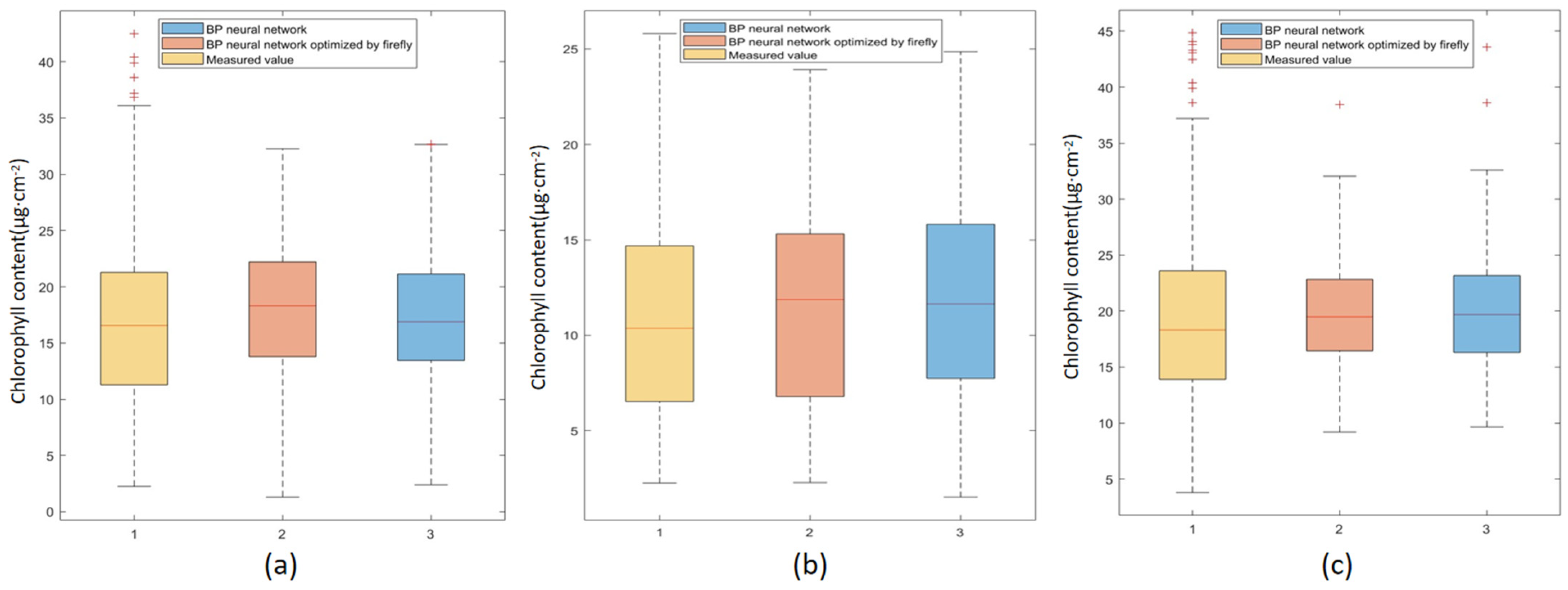
Compared with the traditional time-consuming, labor-intensive, and destructive methods for obtaining forest chlorophyll content, the remote sensing technology of UAVs equipped with hyperspectral sensors and LiDAR shortens the period of data acquisition. In this study, four statistical models were used to estimate the canopy chlorophyll content for three different stand types: coniferous forest, broad-leaved forest, and mixed coniferous broad-leaved forest. The accuracy of the nonlinear random forest model was generally higher than that of the BP neural network, multiple stepwise regression model, and BP neural network optimized by the firefly algorithm. This is because random forests can provide different interpretations of decision trees, resulting in better performance of the model. And the accuracy of the BP neural network model optimized by the firefly algorithm was better than that of the BP neural network. Neural networks require more data to be truly effective, as they can disrupt the interpretability of features. However, compared with the BP neural network, the optimized algorithm can seek the optimal solution of model parameters [50] and pass the optimal parameters to the BP neural network for model construction. It was also found that the accuracy of the mechanism model was excellent, because the physical model could simulate leaf chlorophyll content data under different conditions in nature by inputting complex parameters [22], and the accuracy of the model was less affected by spatial region and time factors. Compared with the statistical model, the mechanism model has higher robustness.

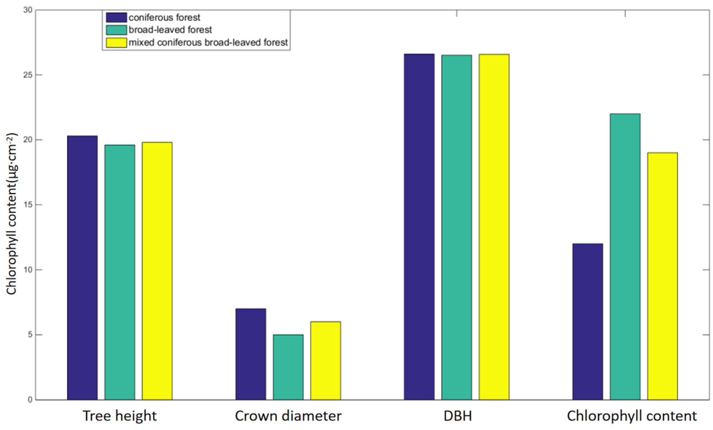
The results of chlorophyll content estimation are significantly different among different stand types. The chlorophyll content is influenced by factors such as light, temperature, moisture, and mineral elements, among which light is a necessary condition for chlorophyll. Under the condition of shading, the relative content of light-collecting pigment protein in the photosynthetic unit increased, which leads to an increase in binding chlorophyll. At the same time, it reduces the degradation and photo-oxidation of chlorophyll; therefore, the content of chlorophyll will increase after shading [54]. 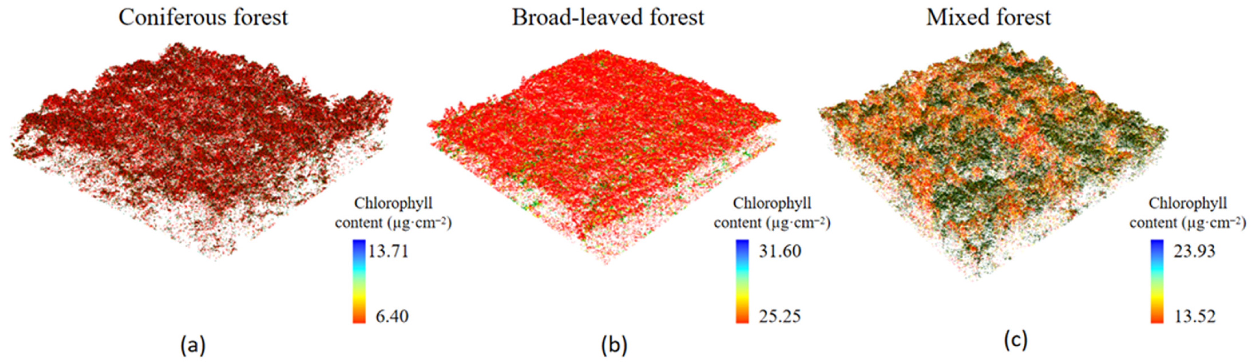When studying the shading rate of trees, Wang concluded that the diameter at breast height and crown width of most tree species were significantly correlated with the shading rate, and most of them were positively correlated [55]. It can be seen from Figure 14 that the broad-leaved forest has the highest chlorophyll content, and the coniferous forest has the lowest. The reason is that the largest crown width is in broad-leaved forests, and the smallest is in coniferous forests. Meanwhile, the largest chest height is in broad-leaved forests, and the smallest is in coniferous forests. Therefore, the forest with the highest shading rate is the broad-leaved forest, and the one with the lowest is the coniferous forest. Studies show that tree height mainly determines the shading range of trees with small solar altitude angles in the morning and evening and has little influence during the main periods of photosynthesis [55]. Therefore, even if the tallest trees are in coniferous forests, and the smallest are in broad-leaved forests, it will not have a significant impact on chlorophyll content. In this study, there is little difference in DBH size among the three tree species, so the main influencing factor is crown diameter.

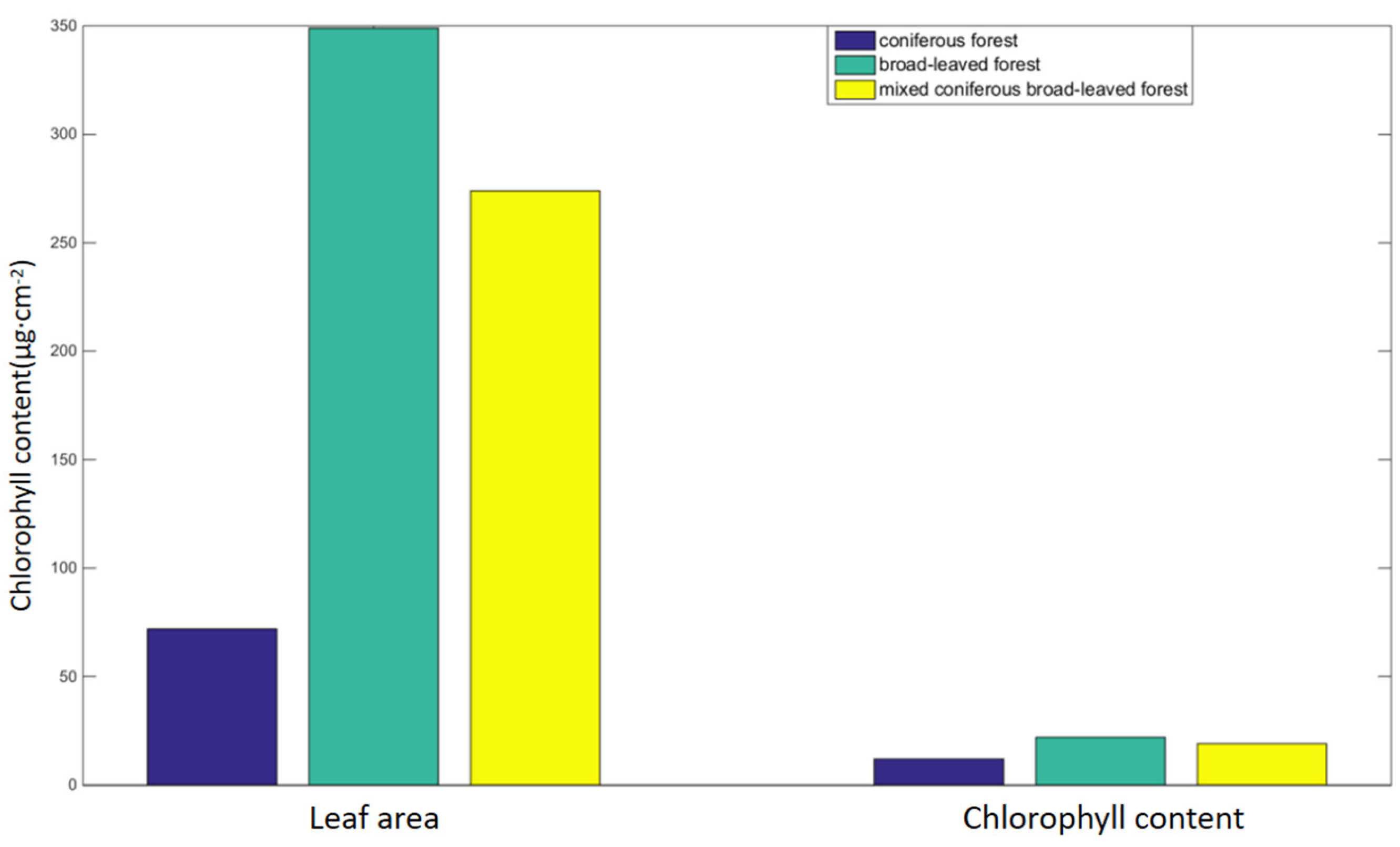
In addition, the leaf shape of trees can also affect chlorophyll content. The common leaf types of coniferous forests are narrow, mostly strip-shaped, and needle-shaped, while those of broad-leaved forests are wide, mostly round, and oval. The leaves of broad and flat broad-leaved trees contain many mesophyll tissues composed of chloroplast parenchyma cells, and the mesophyll tissues are large in quantity and volume, while the long and narrow coniferous mesophyll tissues are folded from green parenchyma tissues, and the number and volume of mesophyll tissues are smaller than those of broad-leaved leaves. According to the research, the larger the leaf area, the more light sources can be obtained by the leaves of plants, which can improve their photosynthetic capacity and correspondingly increase the chlorophyll content [56]. As shown in Figure 15, the size of leaf area in order is broad-leaved forest, mixed coniferous and broad-leaved forest, and coniferous forest. Therefore, the size of photosynthetic area (number and volume of mesophyll tissue) in order is broad-leaved forest, mixed coniferous and broad-leaved forest, and coniferous forest, and the corresponding chlorophyll content in order is broad-leaved forest, mixed coniferous and broad-leaved forest, and coniferous forest.

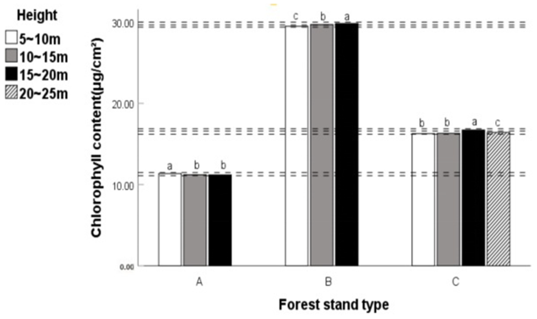
Some researchers found that plants can maximize their light utilization efficiency by using an open crown when studying the impact of plant light utilization capacity on tree architecture [57]. As the sampling height increases, the canopy opening (p < 0.01) of coniferous forests significantly decreases, and correspondingly, the utilization efficiency of light by leaves also decreases. Therefore, the chlorophyll content of coniferous forests decreases with the increase in height. As the sampling height increases, the crown opening of broad-leaved forests (p < 0.05) significantly increases, and the crown opening of coniferous and broad-leaved mixed forests increases. Correspondingly, the utilization efficiency of light by leaves also increases. Therefore, the chlorophyll content of broad-leaved forests and coniferous and broad-leaved mixed forests increases with the increase in height. On the other hand, due to the sparse light that can directly illuminate the lower leaves in coniferous forests, the environmental temperature in which the leaves are located decreases with height. Leaves living in low temperatures increase their cold resistance by reducing the water content in their cells. The reduction in water inhibits the synthesis of chlorophyll, so the chlorophyll content of coniferous forests decreases with the increase in height. On the contrary, broad-leaved forests are often dense, and the light cannot reach the lower leaves, which leads to lower ambient temperatures in the lower leaves, less water in the leaf cells, and correspondingly less chlorophyll content than the upper leaves. The leaves of the broad-leaved tree species in the top layer of the coniferous and broad-leaved mixed forest are exposed to high levels of light radiation, resulting in more water evaporation and being in a water-deficient environment. Therefore, the leaves of broad-leaved tree species can avoid water loss by reducing their light-receiving area. On the other hand, the cuticle layer of the leaves at each level of coniferous tree species is thicker, which can effectively reduce water evaporation. Therefore, there will not be significant differences in the light-receiving area of the leaves at each level [56]. This also explains why the chlorophyll content of leaves in coniferous and broad-leaved mixed forests at a height of 20~25 m is lower than that at a height of 15~20 m.

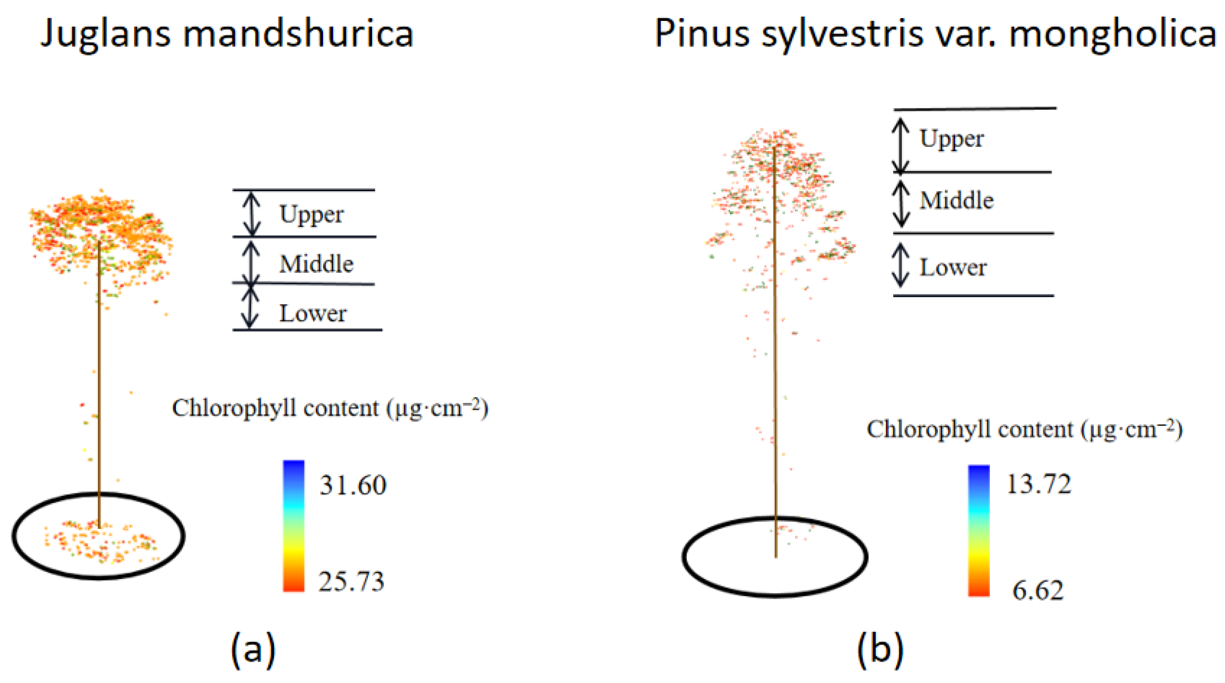
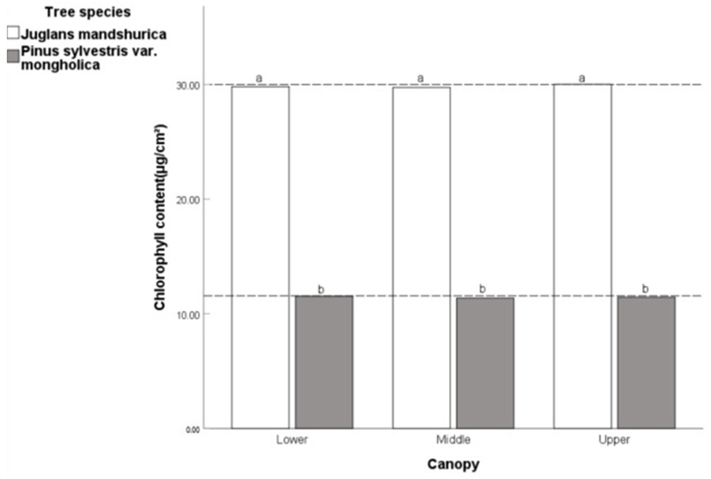
There are differences in the distribution of chlorophyll content in the canopy of different tree species at different levels and heights. The chlorophyll content in the upper layer of Juglans mandshurica is higher than that in the middle and lower layers, while the chlorophyll content in the upper layer of Pinus sylvestris var. mongolica is lower than that in the lower layer. The main reason is that the complex spatial structure of the forest and the difference in the crown shape of the trees themselves lead to uneven distribution of light resources [15]. The limited spatial position makes the trees compete fiercely for light resources [1,2]. The pinnacle crown of Pinus sylvestris var. mongolica makes the light be mainly distributed in the middle and upper layers, and the lower layer can only get a little light. In order to capture more light energy, the leaves of the lower layer can only increase their chlorophyll content for more photosynthesis. The umbrella-shaped crown of Juglans mandshurica makes the leaves concentrate on the upper part of the canopy. As the canopy is divided from the first live branch of the trunk upwards, the number of upper leaves is higher than that of the middle and lower layers when dividing the canopy equally. Coupled with the spatial competition among trees, the number of leaves in the lower layer decreases sharply during the self-thinning process of trees. Secondly, it is difficult for light to penetrate the leaves and branches to reach the middle and lower layers [29] because of the cover of the upper broad-leaved leaves, which reduces the resource allocation of middle and lower layer leaves and leads to a decrease in chlorophyll content in the middle and lower layers. The chlorophyll content of Juglans mandshurica and Pinus sylvestris var. mongolica in the horizontal direction of a single tree is significantly different in the shady and sunny directions, which further shows that the uneven distribution of light energy in the shady and sunny directions affects the chlorophyll distribution.

However, the models studied in this paper are all limited, and all models are based on certain assumptions and simplifications, which may not be completely valid in the actual estimation. This leads to errors in the estimates. At the same time, ecological complexity will also affect the accuracy of the chlorophyll estimation model.

The chlorophyll content can indicate the status of forest productivity [4,5]. The fluctuation of chlorophyll content in coniferous and broad-leaved mixed forests is greater than that in coniferous and broad-leaved forests, indicating that coniferous and broad-leaved mixed forests can adapt well to changes in light and make more full use of light energy. Simultaneously increasing the solidification rate of carbon and enhancing forest productivity. The shortcoming of the study is that the effects of climate change on the chlorophyll content distribution of different stands are not considered. In the future, the effects of climate change on the spatial distribution of chlorophyll content of stands can be evaluated by measuring the chlorophyll content of sample trees by setting plots in different climatic zones.

5. Conclusions

In this study, the chlorophyll content of different stand types and different single tree species was estimated by UAV hyperspectral images combined with LiDAR point cloud data. The results show that the hybrid data-driven mechanism model based on the radiation transmission model PROSPECT is the most robust. Among the statistical models, the random forest has the best accuracy. There are significant differences in chlorophyll content among different forest stand types. In the vertical direction, the chlorophyll content in the upper canopy of coniferous forest is lower than that in the middle and lower canopies, while the chlorophyll content in the upper canopy of broad-leaved forest and mixed forest is higher than that in the middle and lower canopies, and there are differences between different layers. There are significant differences in the distribution of chlorophyll content in the horizontal direction of different tree species on shaded and sunny slopes, and the chlorophyll content inside the canopy is lower than that outside the canopy. In the vertical direction, the chlorophyll content in the upper layer of Juglans mandshurica is higher than that in the middle and lower layers, with a significant difference, while the chlorophyll content in the lower layer of Pinus sylvestris var. mongolica is higher than that in the middle and upper layers, with no significant difference. In summary, this study improved the accuracy of chlorophyll content estimation for individual trees and stands through the optimal model, which provided theoretical support for the accurate estimation of chlorophyll. The fusion of hyperspectral images and LiDAR point clouds to construct a three-dimensional spatial image can estimate the spatial distribution of chlorophyll content at individual trees and different stand levels.

References

1. Niinemets, Ü. Within-canopy variations in functional leaf traits: Structural, chemical and ecological controls and diversity of responses. In Canopy Photosynthesis: From Basics to Applications; Hikosaka, K., Niinemets, Ü., Anten, N.P.R., Eds.; Springer: Dordrecht, The Netherlands, 2016; pp. 101–141. [Google Scholar]
2. Koike, T.; Kitao, M.; Maruyama, Y.; Mori, S.; Lei, T.T. Leaf morphology and photosynthetic adjustments among deciduous broad-leaved trees within the vertical canopy profile. Tree Physiol. 2001, 21, 951–958. [Google Scholar] [CrossRef] [PubMed]
3. He, G.; Wu, J.; Peng, J. A hyperspectral model for estimating chlorophyll content in Photinia leaves. J. Northwest For. Univ. 2022, 37, 25–32. [Google Scholar]
4. Coops, N.C.; Stone, C.; Culvenor, D.S.; Chisholm, L.A.; Merton, R.N. Chlorophyll content in eucalypt vegetation at the leaf and canopy scales as derived from high resolution spectral data. Tree Physiol. 2003, 23, 23–31. [Google Scholar] [CrossRef]
5. Yang, X.G.; Yu, Y.; Fan, W.Y. Chlorophyll content retrieval from hyperspectral remote sensing imagery. Environ. Monit. Assess. 2015, 187, 456. [Google Scholar] [CrossRef] [PubMed]
6. Bussotti, F.; Pollastrini, M. Evaluation of leaf features in forest trees: Methods, techniques, obtainable information and limits. Ecol. Indic. 2015, 52, 219–230. [Google Scholar] [CrossRef]
7. Kai, Z.; Lin, C. The application status and prospects of remote sensing in precise forest cultivation. J. Remote Sens. 2021, 25, 423–438. [Google Scholar]
8. Upadhyay, V.; Kumar, A. Hyperspectral remote sensing of forests: Technological advancements, opportunities and challenges. Earth Sci. Inform. 2018, 11, 487–524. [Google Scholar] [CrossRef]
9. Zhong, Y.; Wang, X.; Xu, Y.; Wang, S.; Jia, T.; Hu, X.; Zhao, J.; Wei, L.; Zhang, L. Mini-UAV-Borne hyperspectral remote sensing: From observation and processing to applications. IEEE Geosci. Remote Sens. Mag. 2018, 6, 46–62. [Google Scholar] [CrossRef]
10. Zhao, G. Application and demand analysis of drone remote sensing in forestry. Fujian For. Technol. 2017, 44, 136–140. [Google Scholar]
11. Li, M.; Liu, Q.; Feng, Y. Analysis of unmanned aerial vehicle LiDAR artificial forest stand overestimation model. J. Remote Sens. 2022, 26, 2665–2678. [Google Scholar]
12. Zhao, Y.; Zeng, Y.; Zheng, Z.; Dong, W.; Zhao, D.; Wu, B.; Zhao, Q. Forest species diversity mapping using airborne LiDAR and hyperspectral data in a subtropical forest in China. Remote Sens. Environ. 2018, 213, 104–114. [Google Scholar] [CrossRef]
13. Li, J.; Li, M.; Quan, Y. Tree species classification in the Mao’er Mountain area using drone LiDAR and hyperspectral data collaboration. J. Northeast For. Univ. 2022, 50, 63–69. [Google Scholar]
14. Liu, Y.; Pang, Y.; Liao, S. Airborne LiDAR and hyperspectral fusion to achieve tree species classification in Pu’er mountainous areas. For. Sci. Res. 2016, 29, 407–412. [Google Scholar]
15. Thomas, V.; Treitz, P.; Mccaughey, J.H.; Noland, T.; Rich, L. Canopy chlorophyll concentration estimation using hyperspectral and lidar data for a boreal mixedwood forest in northern Ontario, Canada. Int. J. Remote Sens. 2008, 29, 1029–1052. [Google Scholar] [CrossRef]
16. Shen, X.; Cao, L.; Coops, N.C.; Fan, H.; Wu, X.; Liu, H.; Wang, G.; Cao, F. Quantifying vertical profiles of biochemical traits for forest plantation species using advanced remote sensing approaches. Remote Sens. Environ. 2020, 250, 112041. [Google Scholar] [CrossRef]
17. Yin, S.; Zhou, K.; Cao, L.; Shen, X. Estimating the horizontal and vertical distributions of pigments in canopies of ginkgo plantation based on UAV-borne LiDAR, hyperspectral data by coupling PROSAIL model. Remote Sens. 2022, 14, 715. [Google Scholar] [CrossRef]
18. Hosoi, F.; Umeyama, S.; Kuo, K. Estimating 3D chlorophyll content distribution of trees using an image fusion method between 2D camera and 3D portable scanning LiDAR. Remote Sens. 2019, 11, 2134. [Google Scholar] [CrossRef]
19. Lin, Q.; Huang, H.; Wang, J.; Huang, K.; Liu, Y. Detection of pine shoot beetle (PSB) stress on pine forests at individual tree level using UAV-based hyperspectral imagery and LiDAR. Remote Sens. 2019, 11, 2540. [Google Scholar] [CrossRef]
20. Ma, Y.; Yang, B.; Zhao, N. A classification and diagnosis study on the degree of damage of Yunnan pine to Yunnan cutting bark beetle based on hyperspectral and airborne LiDAR technology. J. Southwest For. Univ. Nat. Sci. 2022, 42, 80–89. [Google Scholar]
21. Yu, R.; Luo, Y.; Zhou, Q.; Zhang, X.; Wu, D.; Ren, L. A machine learning algorithm to detect pine wilt disease using UAV-based hyperspectral imagery and LiDAR data at the tree level. Int. J. Appl. Earth Obs. Geoinf. 2021, 101, 102363. [Google Scholar] [CrossRef]
22. Xu, J.; Meng, J. Research progress and prospect of crop chlorophyll content estimation by remote sensing. Remote Sens. Technol. Appl. 2016, 31, 74–85. [Google Scholar]
23. Liao, W.Z.; Van Coillie, F.; Gao, L.R.; Chanussot, J. Deep learning for fusion of apex hyperspectral and full-waveform lidar remote sensing data for tree species mapping. IEEE Access 2018, 6, 68716–68729. [Google Scholar] [CrossRef]
24. Liao, W.; Van Coillie, F.; Gao, L.; Li, L.; Zhang, B.; Chanussot, J. Research on the method of ground object extraction by fusing hyperspectral remote sensing images and airborne LiDAR data. Remote Sens. Inf. 2014, 29, 73–76+83. [Google Scholar]
25. Blackburn, G.A. Remote sensing of forest pigments using airborne imaging spectrometer and lidar imagery. Remote Sens. Environ. 2002, 82, 311–321. [Google Scholar] [CrossRef]
26. Koetz, B.; Sun, G.; Morsdorf, F.; Ranson, K.; Kneubühler, M.; Itten, K.; Allgöwer, B. Fusion of imaging spectrometer and lidar data over combined radiative transfer models for forest canopy characterization. Remote Sens. Environ. 2007, 106, 449–459. [Google Scholar] [CrossRef]
27. Impollonia, G.; Croci, M.; Blandinières, H.; Marcone, A.; Amaducci, S. Comparison of PROSAIL model inversion methods for estimating leaf chlorophyll content and LAI using UAV imagery for hemp phenotyping. Remote Sens. 2022, 14, 5801. [Google Scholar] [CrossRef]
28. Wu, B.; Huang, W.; Ye, H.; Luo, P.; Ren, Y.; Kong, W. Using multi-angular hyperspectral data to estimate the vertical distribution of leaf chlorophyll content in wheat. Remote Sens. 2021, 13, 1501. [Google Scholar] [CrossRef]
29. Cervena, L.; Lhotakova, Z.; Kupkova, L.; Kovarova, M.; Albrechtova, J. Models for estimating leaf pigments and relative water content in three vertical canopy levels of Norway spruce based on laboratory spectroscopy. In Proceedings of the 34th EARSeL Symposium, Warsaw, Poland, 16–20 June 2014. [Google Scholar]
30. Xiao, Y.F. Scale Effect and Sensitivity Analysis of Vegetation Physical and Chemical Parameter Inversion. Doctoral Dissertation, Capital Normal University, Beijing, China, 2013. [Google Scholar]
31. Zhao, D.H.; Li, J.L.; Song, Z.J. Research progress on the mechanism and methods of extracting vegetation biochemical parameters by hyperspectral technology. Adv. Earth Sci. 2003, 94–99. [Google Scholar]
32. Jacquemoud, S.; Baret, F. PROSPECT: A model of leaf optical properties spectra. Remote Sens. Environ. 1990, 34, 75–91. [Google Scholar] [CrossRef]
33. Gitelson, A.A.; Merzlyak, M.N.; Lichtenthaler, H.K. Detection of red edge position and chlorophyll content by reflectance measurements near 700 nm. J. Plant Physiol. 1996, 148, 501–508. [Google Scholar] [CrossRef]
34. Gitelson, A.A.; Kaufman, Y.J.; Merzlyak, M.N. Use of a green channel in remote sensing of global vegetation from EOS-MODIS. Remote Sens. Environ. 1996, 58, 289–298. [Google Scholar] [CrossRef]
35. Jordan, C.F. Derivation of leaf-area index from quality of light on the forest floor. Ecology 1969, 50, 663–666. [Google Scholar] [CrossRef]
36. Hunt, E.R.; Cavigelli, M.; Daughtry, C.S.T.; Mcmurtrey, J.E.; Walthall, C.L. Evaluation of digital photography from model aircraft for remote sensing of crop biomass and nitrogen status. Precis. Agric. 2005, 6, 359–378. [Google Scholar] [CrossRef]
37. Rouse, J.W.; Haas, R.H.; Schell, J.A.; Deering, D.W. Monitoring Vegetation Systems in the Great Plains with ERTS; NASA Special Publication: Washington, DC, USA, 1974; p. 351. [Google Scholar]
38. Daughtry, C. Estimating corn leaf chlorophyll concentration from leaf and canopy reflectance. Remote Sens. Environ. 2000, 74, 229–239. [Google Scholar] [CrossRef]
39. Huete, A.; Didan, K.; Miura, T.; Rodriguez, E.P.; Gao, X.; Ferreira, L.G. Overview of the radiometric and biophysical performance of the MODIS vegetation indices. Remote Sens. Environ. 2002, 83, 195–213. [Google Scholar] [CrossRef]
40. Penuelas, J.; Baret, F.; Filella, I. Emi-empirical indices to assess carotenoids/chlorophyll a ratio from leaf spectral reflectances. Photosynthetica 1995, 31, 221–230. [Google Scholar]
41. Kim, M.S.; Daughtry, C.S.T.; Chappelle, E.W.; Mcmurtrey, J.E.; Walthall, C.L. The use of high spectral resolution bands for estimating absorbed photosynthetically active radiation. In Proceedings of the 6th International Symposium on Physical Measurements and Signatures in Remote Sensing, Val D’Isere, France, 17–21 January 1994; pp. 299–306. [Google Scholar]
42. Haboudane, D.; Miller, J.R.; Tremblay, N.; Zarco-Tejada, P.J.; Dextraze, L. Integrated narrow-band vegetation indices for prediction of crop chlorophyll content for application to precision agriculture. Remote Sens. Environ. 2002, 81, 416–426. [Google Scholar] [CrossRef]
43. Gamon, J.A.; Serrano, L.; Surfus, J.S. The photochemical reflectance index: An optical indicator of photosynthetic radiation use efficiency across species, functional types, and nutrient levels. Oecologia 1997, 112, 492–501. [Google Scholar] [CrossRef]
44. Merzlyak, M.N.; Gitelson, A.A.; Chivkunova, O.B.; Rakitin, V.Y. Non-destructive optical detection of pigment changes during leaf senescence and fruit ripening. Physiol. Plant. 1999, 106, 135–141. [Google Scholar] [CrossRef]
45. Cui, B. Research on Forest Volume Estimation Based on Machine Learning; Central South University of Forestry and Technology: Changsha, China, 2022. [Google Scholar]
46. Gao, L. Estimation of Aboveground Biomass in Plantations by Integrating Airborne LiDAR and Hyperspectral Data; Beijing Forestry University: Beijing, China, 2021. [Google Scholar]
47. Ju, Y.; Ji, Y.; Huang, J.; Zhang, W. Research on the inversion of forest aboveground biomass by combining LiDAR and multispectral data. J. Nanjing For. Univ. (Nat. Sci. Ed.) 2022, 46, 58–68. [Google Scholar]
48. Shen, X.; Cao, L.; She, G. Inversion of subtropical forest biomass using hyperspectral and high spatial resolution remote sensing data. J. Remote Sens. 2016, 20, 1446–1460. [Google Scholar]
49. Li, K.; Chen, Y.; Xu, Z.; Hu, X.; Wang, X. Hyperspectral estimation method of chlorophyll content in Phyllostachys edulis under pest stress. Spectrosc. Spectr. Anal. 2020, 40, 2578–2583. [Google Scholar]
50. Lu, B.; He, Y. Evaluating empirical regression, machine learning, and radiative transfer modelling for estimating vegetation chlorophyll content using bi-seasonal hyperspectral images. Remote Sens. 2019, 11, 1979. [Google Scholar] [CrossRef]
51. Yang, X.S. Firefly algorithms for multimodal optimization. In Proceedings of the 5th International Conference on Stochastic Algorithms: Foundations and Applications, Sapporo, Japan, 26–28 October 2009; Watanabe, O., Zeugmann, T., Eds.; Springer-Verlag: Berlin/Heidelberg, Germany, 2009; pp. 169–178. [Google Scholar]
52. Wang, D.; Luo, H.; Grunder, O.; Lin, Y.; Guo, H. Multi-step ahead electricity price forecasting using a hybrid model based on two-layer decomposition technique and BP neural network optimized by firefly algorithm. Appl. Energy 2017, 190, 390–407. [Google Scholar] [CrossRef]
53. Li, D.; Chen, J.M.; Zhang, X.; Yan, Y.; Zhu, J.; Zheng, H.; Zhou, K.; Yao, X.; Tian, Y.; Zhu, Y.; et al. Improved estimation of leaf chlorophyll content of row crops from canopy reflectance spectra through minimizing canopy structural effects and optimizing off-noon observation time. Remote Sens. Environ. 2020, 248, 111985. [Google Scholar] [CrossRef]
54. Wang, X. Analysis of the impact of shading on photosynthesis. Mod. Agric. Sci. Technol. 2013, 74. [Google Scholar]
55. Wang, R.; Yang, J.; Cheng, Y. The shading rate of urban green trees in Nanjing. China Urban For. 2020, 18, 40–45. [Google Scholar]
56. Tian, J.; Wei, L.; He, N. Changes in leaf traits of temperate coniferous broad-leaved mixed forests with vertical crown height. J. Ecol. 2018, 38. [Google Scholar]
57. Yang, X. The Effects of Light Utilization and Water Transport Capacity of Evergreen Broad-Leaved Forest Plants on the Vertical Hierarchy of Tree Architecture; East China Normal University: Shanghai, China, 2015. [Google Scholar]
Figure 1. Spatial distribution of study area.
Remotesensing 17 01699 g001
Figure 2. Watershed segmentation method.
Remotesensing 17 01699 g002
Figure 3. BP neural network.
Remotesensing 17 01699 g003
Figure 4. Results of sensitivity analysis: I: Chlorophyll content. II: Carotenoid content. III: Structural parameter. IV: Equivalent water thickness. V: Dry matter content.
Remotesensing 17 01699 g004
Figure 5. Correlation coefficients of chlorophyll with leaf spectrum, leaf spectrum logarithm: (a) Correlation between spectral logarithm and chlorophyll. (b) Correlation between leaf spectral and chlorophyll. I: Coniferous and broad-leaved mixed forest. II: Coniferous forest. III: Broad-leaved forest. IV: Mixed sample of PROSPECT and measured data. The same below.
Remotesensing 17 01699 g005
Figure 6. Importance of random forest model variables for different forest types: (a) Coniferous forest. (b) Broad-leaved forest. (c) Mixed forest. (d) PROSPECT mixed data.
Remotesensing 17 01699 g006
Figure 7. Random forest model fitting results: (a) Mixed forest. (b) Broad-leaved forest. (c) Coniferous forest. (d) Mixed sample of PROSPECT and measured data. (e) Validation of the low chlorophyll value region. (f) Validation of the high chlorophyll value region.
Remotesensing 17 01699 g007
Figure 8. Standardized residual analysis plot of random forest.
Remotesensing 17 01699 g008
Figure 9. Fitting results of BP neural network and BP neural network optimized by firefly algorithm models: (a) mixed coniferous and broad-leaved forests; (b) coniferous forests; and (c) broad-leaved forests.
Remotesensing 17 01699 g009
Figure 10. Vertical distribution of chlorophyll of different tree species: (a) Juglans mandshurica and (b) Pinus sylvestris var. mongolica.
Remotesensing 17 01699 g010
Figure 11. Chlorophyll content in the vertical layer of different tree species. a and b indicated significant difference at 0.05 level.
Remotesensing 17 01699 g011
Figure 12. Three-dimensional spatial distribution of chlorophyll for three forest types: (a) Coniferous forest. (b) Broad-leaved forest. (c) Mixed forest.
Remotesensing 17 01699 g012
Figure 13. Vertical distribution of chlorophyll content for different forest types. a, b and c indicated significant difference at 0.05 level.
Remotesensing 17 01699 g013
Figure 14. The chlorophyll content is related to leaf area in different forest stand types.
Remotesensing 17 01699 g014
Figure 15. The chlorophyll content is related to diameter at breast height, crown width, and tree height in different forest stand types.
Remotesensing 17 01699 g015