1. Introduction
SLAM is a key technology enabling self-awareness in intelligent mobile devices, with applications in fields like mobile robots, drones, and so on [
1,
2]. While GNSS-based navigation systems have been widely adopted in open environments, their positioning accuracy severely degrades in denied environments such as indoor spaces, urban canyons, and underground tunnels due to signal occlusion or interference [
3,
4]. This limitation has driven significant research interest in alternative localization methods, particularly visual SLAM, which leverages the ubiquity and low cost of cameras to achieve environment-aware positioning without relying on external signals [
5]. Due to the increasing number of visual SLAM systems being developed, the challenge of performing well in GNSS-denied environments has been addressed, some of which include PTAM [
6], ORB-SLAM2 [
7], VINS-Mono [
8], and ORB-SLAM3 [
9].
However, visual SLAM’s applicability is limited by its reliance on a static environment assumption, which restricts its use in real-world scenarios. Dynamic environments in real applications introduce numerous erroneous correspondences, resulting in an inaccurate state estimation in visual SLAM systems [
10,
11]. Although the algorithms for generalizing SLAM systems perform well in certain scenarios, they still encounter issues when dealing with dynamic objects. In recent years, various methods for dealing with dynamic objects have been presented. These include deep learning-based methods and geometry-based approaches as well as hybrid methods.
Most existing geometry-based methods that are used for dealing with dynamic objects rely on the information collected from rigid objects and motion consistency. Kim et al. [
12] proposed a dense visual odometry method that used an RGB-D camera to estimate the sensor’s ego-motion. Wang et al. [
13] utilized an RGB-D algorithm for detecting moving objects in an indoor environment that was able to achieve an improved performance by taking into account geometric constraints and mathematical models. Geometry-based methods usually depend on predefined thresholds to eliminate dynamic feature points, often leading to over-detection or under-detection.
Methods for deep learning that are used for removing dynamic features rely on semantic data collected from images [
14]. Li et al. [
15] proposed a system that used semantic segmentation and mixed information fusion to improve its localization accuracy and remove dynamic feature points. Xiao et al. [
16] proposed a dynamic object detection method using an SSD object detector with prior knowledge and a compensation algorithm to enhance the recall rate. They also developed a feature-based visual SLAM system that minimized pose estimation errors by selectively tracking dynamic objects. Liu et al. [
17] presented a dynamic SLAM algorithm based on the ORB-SLAM3 framework. It could perform better in real-time tracking accuracy when dealing with complex environments. The reliance on prior knowledge can lead to errors in deep learning such as when it mistakenly recognizes a static object as a dynamic one [
18]. Simple networks may not recognize complex dynamic objects effectively, while complex networks may affect the system’s real-time performance.
Combining geometric methods with deep learning can fully leverage the strengths of both approaches Dynamic environments are first extracted from deep learning, and these methods then refine the extracted semantic information using geometric constraints. Bescos et al. [
19] presented the DynaSLAM framework, which is an extension of ORB-SLAM2. It features multi-view geometry and masks-RCNN for removing dynamic points. In a previous paper, Zhao et al. [
20] proposed a workflow that enabled the accurate segmenting of objects in dynamic environments. Yang et al. [
21] first identified predefined dynamic targets using object detection models and then verified the depth information of dynamic pixels through multi-view constraints. Wu et al. [
22] proposed YOLO-SLAM, which filtered dynamic feature points with Darknet19-YOLOv3 and geometric constraints. Wang et al. [
23] proposed an algorithm combining semantic segmentation and geometric constraints to improve SLAM accuracy in dynamic indoor environments.
Although the methods above-mentioned have achieved significant improvements in accuracy, they still have the following limitations:
- (1)
Systems that rely on semantic information often face difficulties in detecting unknown dynamic features. For example, chairs are typically considered static in semantic labels, but the system may fail to identify this dynamic behavior if they move.
- (2)
The misclassification of stationary dynamic objects as dynamic can lead to excessive feature point removal and affect the data integrity. For example, a person sitting on a chair may be mistakenly identified as a dynamic object.
- (3)
The complexity of semantic segmentation networks leads to inadequate real-time performance and reduced processing efficiency.
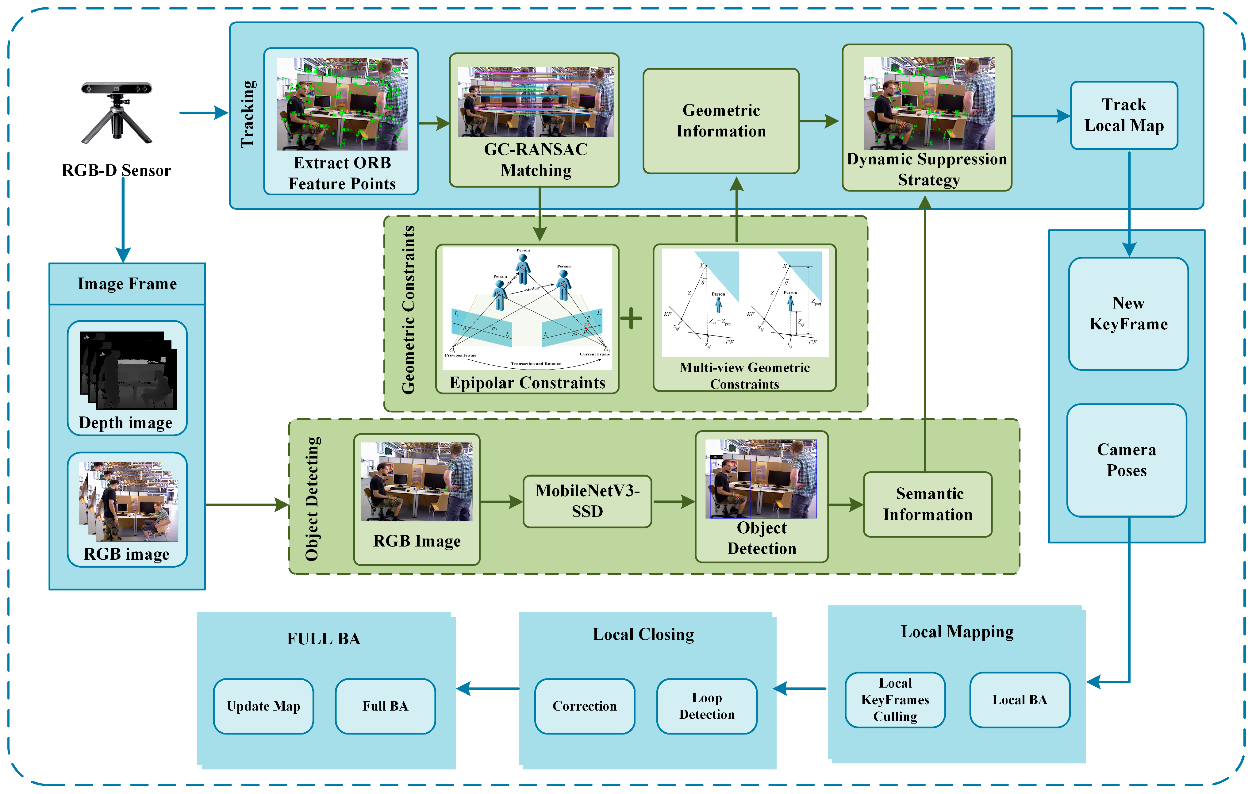
The EMS-SLAM is an improved SLAM algorithm that adopts an RGB-D structure and addresses the limitations and disadvantages of the current methods. This method incorporates geometric constraints and semantic information to suppress dynamic points. In addition to being able to adapt to complex environments, it also meets the requirements of real-time applications. The EMS-SLAM system framework is shown in
Figure 1. The main contributions it makes are summarized below.
- (1)
A feature matching algorithm leveraging graph-cut RANSAC for accurately estimating the pose of cameras;
- (2)
A degeneracy-resistant geometric constraint method that combines epipolar constraints with multi-view geometric constraints, effectively resolving the degeneracy issues inherent in purely epipolar approaches;
- (3)
EMS-SLAM, a real-time RGB-D SLAM system driven by an RGB-D sensor, is constructed. A new parallel thread is integrated into EMS-SLAM to extract semantic information;
- (4)
A dynamic feature suppression algorithm is proposed that combines the advantages of geometric and semantic constraints to efficiently suppress dynamic points. The proposed method can greatly enhance the system’s capability to adapt to complex environments and ensure a stable and accurate performance.
2. Method
2.1. System Framework
The widely used ORB-SLAM2 system is a high-accuracy visual SLAM that includes three main components: loop-closing, tracking, and local mapping. Building on this foundation, EMS-SLAM has been enhanced for dynamic environments by incorporating additional functional modules.
Figure 1 illustrates the EMS-SLAM architecture, which consists of four synchronized threads: tracking, object detection, local mapping, and loop closing.
In EMS-SLAM, RGB-D camera frames are simultaneously processed by the tracking and object detection threads during operation. Within the tracking thread, the RGB image is used to extract ORB feature points. These features are then processed using a GC-RANSAC matching method to ensure the accurate identification of inliers and outliers. The fundamental matrix between frames is then computed using the inlier points, and the fundamental matrix is then used as prior for the geometric constraints. The object detection thread employs a MobileNetV3-SSD model to detect objects in the scene. The object detection thread detects objects in the image and filters out dynamic ones. Since object detection is computationally intensive, the tracking thread has to wait for detection results after calculating the geometric information. To reduce latency, a lightweight object detection model is instead of the semantic segmentation model, which significantly reduces the processing delay.
Subsequently, the tracking thread accurately filters out dynamic points using the dynamic point suppression strategy and utilizes the remaining static points to estimate the camera’s pose. The system then transitions to the local mapping and loop closure threads. Finally, bundle adjustment optimization is carried out to improve the trajectory’s accuracy and system performance.
2.2. Object Detection
In the EMS-SLAM, we used MobileNetV3-SSD to extract semantic information from the input RGB image. The SSD algorithm, proposed by Liu et al. [
24] in 2016, effectively balances the detection speed and accuracy. MobileNetV3 [
25], a lightweight model introduced by Google in 2019, builds upon its predecessors to achieve high detection accuracy with minimal memory usage. Because SSD’s base network, VGG16, has numerous parameters and is unsuitable for embedded platforms, we replaced it with MobileNetV3 to construct the MobileNetV3-SSD object detection model.
We selected NCNN as the inference framework for efficient inference on mobile devices and embedded platforms. NCNN’s optimizations allow the MobileNetV3-SSD model to perform object detection with low latency and high computational efficiency. The training of the model was carried out on the PASCAL VOC 2007 dataset, which ensured its generalizability across different scenarios.
2.3. Feature Matching Method Based on GC-RANSAC
In SLAM systems, the accuracy of the initial pose estimation is important [
26,
27]. However, in dynamic environments, moving objects can lead to feature point mismatches, compromising the pose estimation accuracy. In order to improve the accuracy of the initial pose estimation, we proposed a method that uses the GC-RANSAC algorithm [
28]. Our method addresses the problem of separating inliers and outliers through geometric and spatial consistency to improve the feature point identification accuracy.
We employed the epipolar constraint to determine whether a pair of matching points was an inlier or an outlier. Between two consecutive frames, for a given pair of matching points
, they must satisfy the epipolar constraint
, where
is the epipolar line corresponding to
in the other view, computed from the fundamental matrix
. The RANSAC algorithm’s iterative iteration process classifies the matching point pairs into outliers or inliers according to their constraint. The classification is achieved by optimizing the following energy function:
where
denotes the label assignment for the matching point
, and
represents the neighborhood graph.
The unary term
represents the geometric relationship, defined as:
and
where
is the angle parameter of the fundamental matrix
,
represents the distance between the fundamental matrix and the matching point,
is the inlier–outlier threshold, and the function is a Gaussian kernel function.
indicates that the matching point
is an inlier; otherwise, it is an outlier.
The pairwise term
is used to describe the spatial consistency between neighboring feature points, defined as:
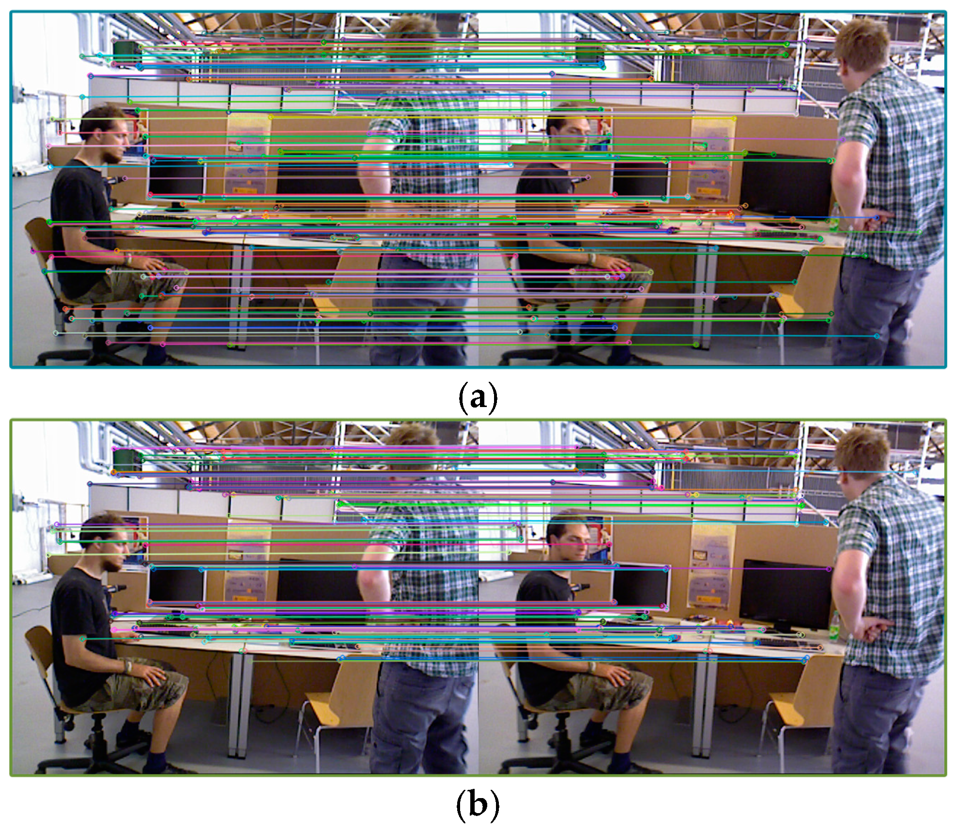
By minimizing this energy function, the GC-RANSAC algorithm effectively separates inliers and outliers [
29]. We then used the inliers to estimate the fundamental matrix
, providing accurate prior information for the epipolar constraints and enhancing the accuracy in filtering out dynamic feature points.
Figure 2 illustrates an example of inlier selection using our proposed method, with the procedure summarized in Algorithm 1.
| Algorithm 1 Feature Matching Method Based on GC-RANSAC |
| Input: | : Previous frame; : Current frame; : Reference frame. |
| Output: | : The fundamental matrix |
| 1: Match features between frames and |
| 2: Get static feature points by GC-RANSAC |
| 3: for each static feature point in do |
| 4: ← FindCorresponding3DPoint(,) |
| 5: end for |
| 6: Estimate fundamental matrix by GC-RANSAC |
| 7: return |
2.4. Epipolar Constraints
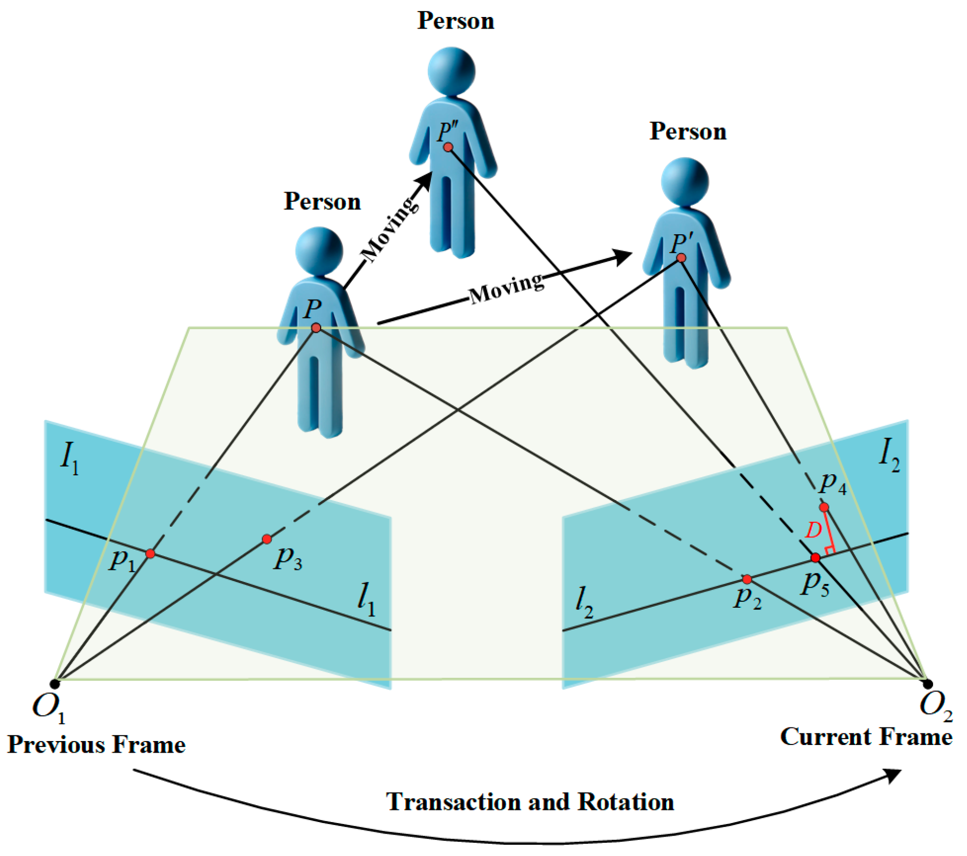
In dynamic environments, current networks can recognize object classes but cannot identify their motion status. Therefore, to eliminate dynamic points originating from static objects, we make full use of epipolar constraints to determine the motion state of feature points. The distance between the feature points and their epipolar lines is calculated, and the points that exceed a certain threshold are regarded as dynamic.
Figure 3 illustrates the optical centers of the cameras, denoted as
and
. The lines
and
represent the epipolar lines. The spatial point
corresponds to the feature points
and
observed in the previous and current frames, respectively:
The coordinate
and
of the feature points of the two frames are shown in the above equation. Their corresponding homogeneous coordinates are:
The epipolar line
can be determined as follows in the current frame:
where
,
,
represent the line vector components, and
represents the fundamental matrix. The epipolar constraints can be expressed as:
The deviation distance
of feature point
to epipolar line
is defined as follows:
The spatial point can be static or dynamic. If it is static, the corresponding feature point in the current frame is , and its deviation distance is . On the other hand, if it is dynamic, the corresponding feature point is , and its deviation distance is .
Figure 3 shows that if a point
is static, its feature point
should be on the epipolar line
. However, due to the noise in the environment, its deviation is not always zero but within the empirical threshold
. When the point moves, its distance
between the epipolar line and the feature point can be calculated. This is used to determine the dynamic state of the feature.
When point moves along the epipolar direction to , its corresponding feature point lies on epipolar line . Therefore, epipolar constraints cannot effectively identify these dynamic objects in such cases. To address this issue, we introduced multi-view geometric constraints, building on epipolar constraints, to detect further missed dynamic feature points.
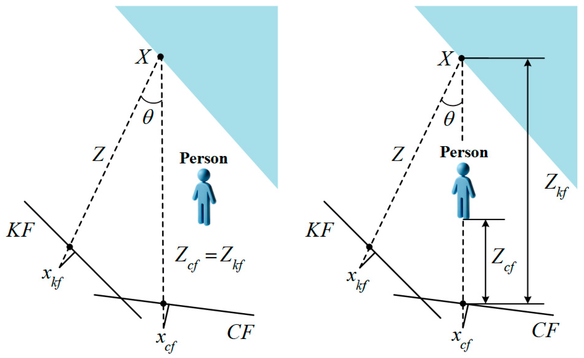
2.5. Muti-View Geometric Constraints
Dynamic scenes create significant changes in the angle and depth of the feature points in the reference frames and current scenes. Dynamic feature points can be eliminated using angular and depth information. This principle is shown in
Figure 4.
Figure 4 shows that the keyframe feature point
in the reference frame is projected onto the current frame to obtain the feature point
and its projected depth
, generating the corresponding 3D point
. The depth information is obtained by calculating the depth value
and
in the current frame. The depth difference
is defined as
. The angular deviation
is the angle between the reprojections of
and
, which is determined using the cosine rule.
By combining the depth information and angular deviation, a feature point is identified as dynamic under multi-view geometric constraints when the depth difference exceeds the threshold or the angular deviation exceeds the threshold . Here, and are the depth and angular thresholds, respectively.
2.6. Dynamic Feature Suppression Method
This paper proposed a geometric information-based dynamic feature suppression method aimed at reducing the over-reliance on depth learning. First, the target category in formation obtained through the detection module was used as prior knowledge for the system to distinguish between moving and non-moving objects. Since different object categories exhibit distinct motion characteristics, the system assigns each feature point a weight based on its object category, with values ranging from 0 to 1. Indoor objects were classified into three categories based on their motion status: active motion, passive motion, and absolutely static, with different weights assigned to each category. The classification details are shown in
Table 1.
Subsequently, epipolar constraints were used to calculate the distance between feature points and their associated epipolar lines, which was then integrated with feature weights for a more refined comparison. If the distance was below the threshold, it underwent multi-view geometric analysis to examine the angle and depth changes, further determining whether it was dynamic or static. If the distance was below the empirical threshold, the point underwent multi-view geometric analysis to examine the changes in depth and angle, further determining whether it was dynamic or static. By applying these rules, the system can accurately determine the status of all feature points in the current frame. Algorithm 2 provides a detailed explanation of the suppression strategy for dynamic feature points.
| Algorithm 2 Dynamic Feature Rejection Strategy |
| Input: | : Previous frame; : Current frame; : Previous frame’s feature points; : Current frame’s feature points; Depth image; Standard empirical thresholds;: The fundamental matrix. |
| Output: | : Static feature points in the current frame. |
| 1: ReferenceFrames ← ComputeReferenceFrames() |
| 2: for each matched pair (,) in , do: |
| 3: if dynamic object exists and is in a dynamic area then |
| if epipolar line distance and movement probability is within threshold then |
| Compute3DPointInReferenceFrames() |
| if depth and angle are within thresholds then |
| ← |
| end if |
| end if |
| else |
| if epipolar line distance is within threshold then |
| Compute3DPointInReferenceFrames() |
| if depth and angle are within thresholds then |
| ← |
| end if |
| 8: end if |
| 9: end if |
| 18: end for |
| 18: return |
3. Results
This section presents an evaluation of the performance of the system using publicly available TUM RGB-D [
30] and Bonn RGB-D [
31] datasets. Subsequently, ablation and comparative experiments were performed to validate the effectiveness of each module in the dynamic scenes. Additionally, we tested the algorithm on self-collected data. Finally, an in-depth analysis of the system’s real-time performance was carried out. We used the relative pose error (RPE) and absolute trajectory error (ATE) to evaluate the accuracy of SLAM. The optimal results for each sequence have been highlighted in bold. To address uncertainties in object detection and feature extraction, each algorithm was tested ten times per sequence, and the median value was taken as the final result. All experiments were conducted on a computer running Ubuntu 18.04, equipped with an Intel i7-9750H (2.60 GHz) CPU, an NVIDIA GeForce GTX 1660 GPU, and 16 GB of RAM.
3.1. Evaluation on the TUM RGB-D Dataset
In 2012, the TUM group released the RGB-D dataset, which has since become a standard in the SLAM sector. The dataset features various dynamic scenes, each with its own accurate ground truth trajectory. It was obtained through the use of a high-accuracy capture system. We tested EMS-SLAM by performing five dynamic scenes. Among these, the sitting sequence featured a person sitting in a chair with slight limb movement, representing a low-dynamic environment, while the walking sequence featured a person walking continuously, representing a high-dynamic environment.
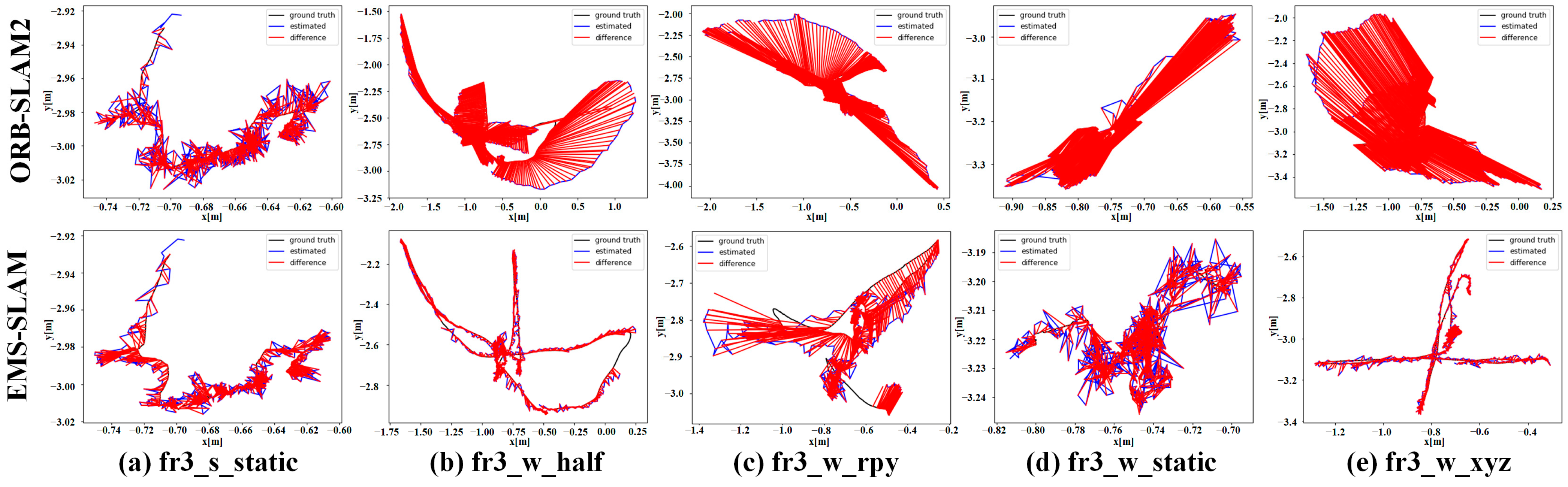
EMS-SLAM was compared with ORB-SLAM2 to assess performance improvements, as shown in
Figure 5 and
Figure 6. As indicated by the ATE results in
Table 2, in high-dynamic sequences, EMS-SLAM achieved a 96.36% improvement in average RMSE accuracy compared with ORB-SLAM2, while the improvement in low-dynamic sequences was 55.17%. This was due to the smaller size and limited movement of dynamic objects in low-dynamic sequences. The RPE results in
Table 3 and
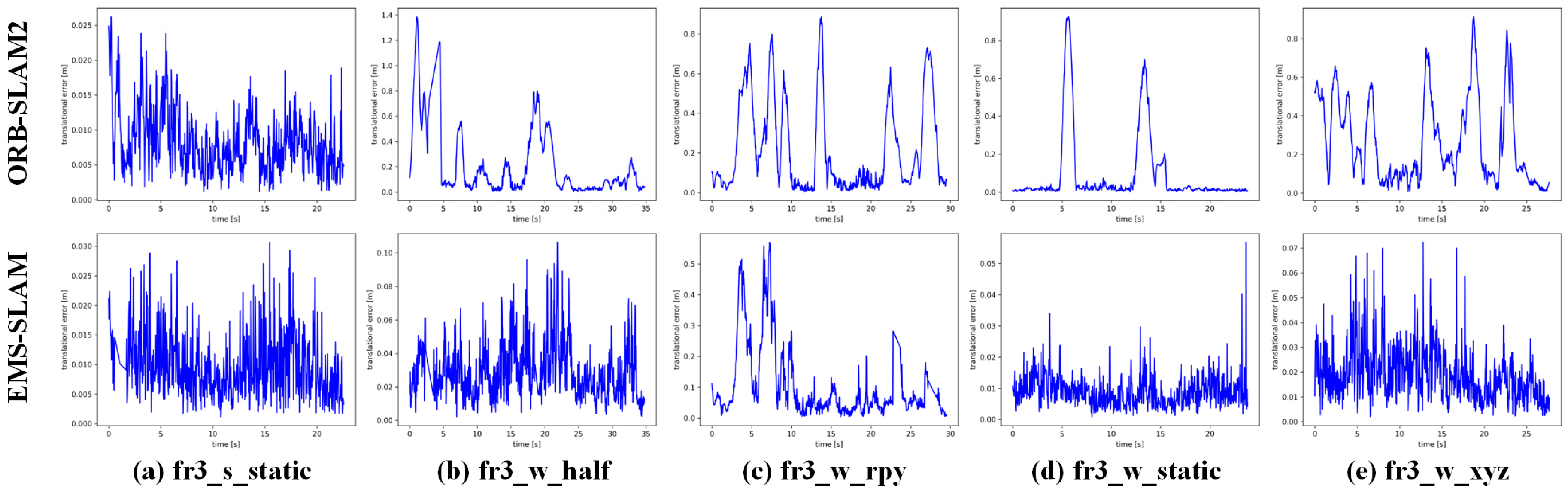
Table 4 indicate that the accuracy of the RMSE was significantly improved by EMS-SLAM compared with ORB-SLAM2. In high-dynamic sequences, the RMSE accuracy improvement was 93.07% and 86.92%, while in low-dynamic instances, it was 47.31% and 46.99%, respectively.
These findings highlight the system’s effectiveness in high-dynamic sequences, with limited improvement in low-dynamic scenarios due to the minimal impact of dynamic objects on SLAM. The ATE results presented in
Figure 5 highlight the differences between the ground-truth and estimated trajectories. EMS-SLAM significantly improved the accuracy compared with ORB-SLAM2.
Figure 6 presents the RPE results, where EMS-SLAM showed reduced errors.
The proposed algorithm was further evaluated by comparing its performance with other mainstream SLAM systems including DSLAM [
32], RS-SLAM [
33], DS-SLAM [
34], RDS-SLAM [
32], RDMO-SLAM [
35], Blitz-SLAM [
36], YOLO-SLAM [
22], and SG-SLAM [
37].
Table 5 presents the experimental results for five dynamic scene sequences. Aside from the fr3_w_static sequence, where EMS-SLAM performed slightly worse than RDMO-SLAM, it achieved a higher average accuracy than other algorithms across the remaining sequences.
3.2. Evaluation on the Bonn RGB-D Dataset
The University of Bonn’s Robotics and Photogrammetry Laboratory released the Bonn RGB-D Dynamic Dataset in 2019, which features 24 dynamic sequences that can be used for various scenarios such as walking people and moving objects. These sequences were recorded using ground-truth camera trajectories from OptiTrack Prime 13. Nine representative sequences were selected to evaluate the system performance. In the crowd sequence, three people were simulated walking randomly indoors, while the moving_no_box sequence depicted the process of moving a box from the ground to a table without obstructing the line of sight. In the person_tracking sequence, the camera followed a slow-moving individual, and in the synchronous sequence, two people were shown moving at the same speed and in the same direction. These highly dynamic scenes present significant challenges for traditional SLAM systems.
The EMS-SLAM system was compared with three standard SLAM systems to verify its robustness and accuracy: ORB-SLAM2, SG-SLAM, and YOLO-SLAM. The evaluation results of the nine scene sequences are presented in
Table 6. In the crowd3 sequence, frequent mutual occlusions, overlapping actions, and changing viewpoints among people in the scene led to false positives and missed detections, affecting the overall performance of the algorithm. In the synchronous2 sequence, the dynamic objects moved synchronously at similar speeds and in the same direction, causing the motion differences relied upon by the epipolar constraints to become indistinct, which in turn affected the accuracy of the motion estimation. Although EMS-SLAM’s performance was slightly inferior to other algorithms on the crowd3 and synchronous2 sequences, EMS-SLAM significantly outperformed the other algorithms in the remaining sequences. These results not only further highlight the EMS-SLAM system’s exceptional accuracy and robustness in dynamic environments, but also showcase its generalization ability across various complex dynamic scenarios.
3.3. Effectiveness Validation of Each Module
3.3.1. Ablation Experiments
The experiments were performed to evaluate the performance of the multi-view geometric and feature matching modules in the TUM RGB-D dataset. Trajectory estimation results were compared across three configurations: EMS-SLAM without the improved feature matching module, EMS-SLAM without the multi-view geometric module, and the complete EMS-SLAM system.
The results of the ablation procedures presented in
Table 7 are shown in detail. The system’s performance in highly dynamic sequences was 36.37% higher than that of the configuration without GC-RANSAC. In contrast, in low-dynamic sequences, the performance was 30.23% lower. Compared with the system without the multi-view geometric algorithm, the complete system achieved an average improvement of 24.68% in highly dynamic sequences and 10.23% in low-dynamic sequences. The main reason is that the smaller dynamic areas and magnitudes reduced the impact of geometric constraints in low-dynamic sequences.
3.3.2. Comparative Experiments
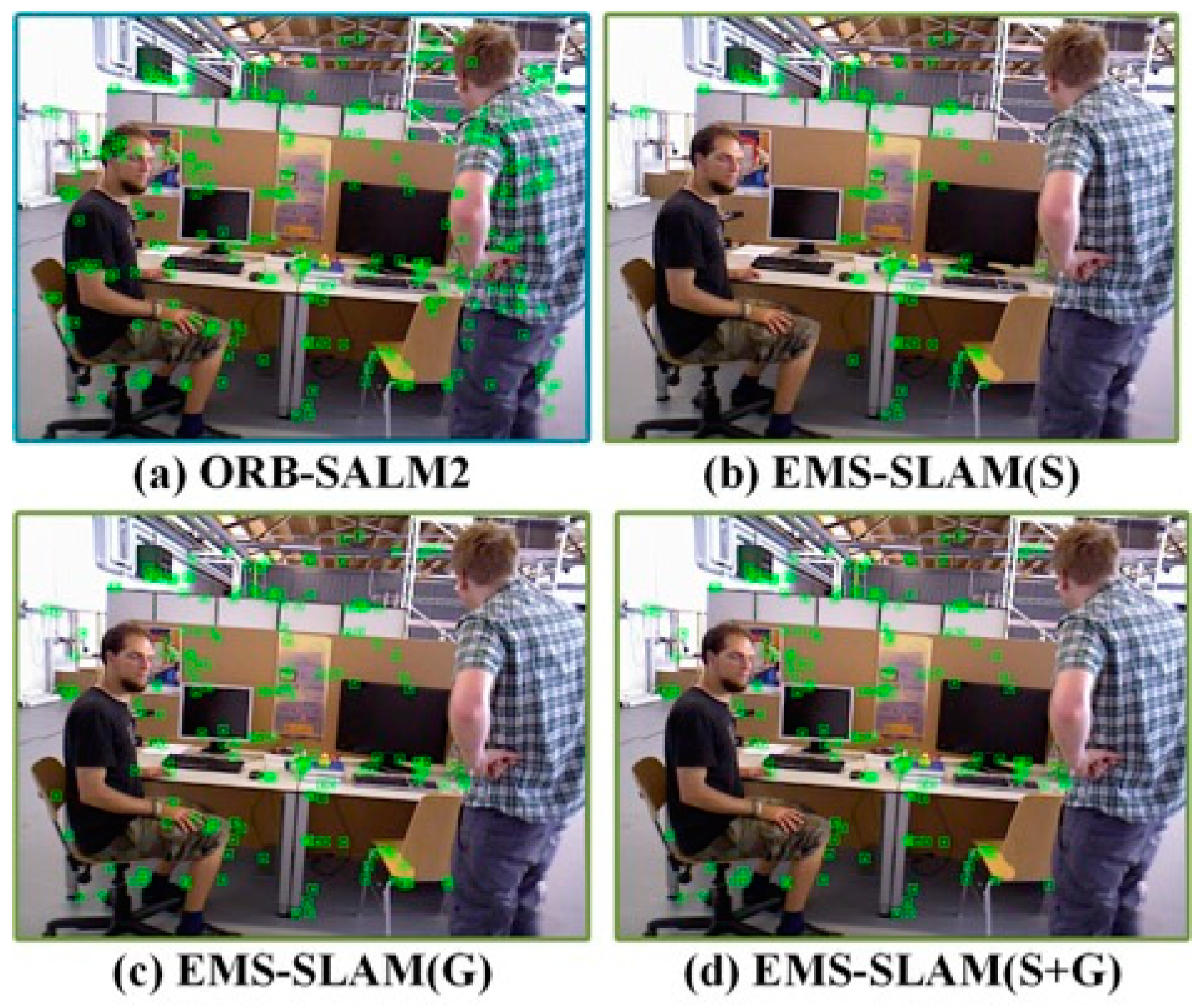
The experiments were conducted to evaluate the effectiveness of the dynamic feature suppression strategy. Three different approaches were used: a geometric algorithm, a semantic algorithm, and a combined algorithm. The results of the experiments are shown in
Figure 7 and show the effectiveness of the different approaches in detecting dynamic points.
- (1)
EMS-SLAM (S): Removes dynamic feature points only using semantic information.
- (2)
EMS-SLAM (G): Removes dynamic feature points only using geometric information.
- (3)
EMS-SLAM (S+G): Removes dynamic feature points by combining semantic and geometric information.
The results, shown in
Figure 7 and
Table 8, demonstrate the comparative performance of each method. ORB-SLAM2, which does not handle dynamic features, indiscriminately extracted feature points in dynamic areas. EMS-SLAM (S), using only semantic information, misclassified many static feature points as dynamic such as those on a computer monitor. EMS-SLAM (G), relying on geometric information, still misidentified some dynamic features as static such as those on a person’s knee while seated. In contrast, EMS-SLAM (S+G), combining semantic and geometric information, effectively removed all dynamic features associated with moving objects while retaining the static object features, outperforming both of the other algorithms.
The two algorithms based on individual information had different strengths and weaknesses across sequences. In contrast, the algorithm delivered the best results in all test sequences by combining the geometric and semantic information. However, in the fr3_w_rpy sequence, complex camera movements caused dynamic objects to blur, resulting in the geometric algorithm having significantly lower errors than the semantic and combined algorithms. Based on the experimental results in
Table 8, in high-dynamic scenes, the combination of semantic and geometric methods improved the RMSE accuracy by 79.17% and 8.70%, respectively, when compared with the semantic or geometric methods individually. In low-dynamic scenes, the combined method yielded results that were nearly identical to those obtained using semantic or geometric methods alone. This suggests that the integration of semantic and geometric information effectively compensates for the limitations of each method, thereby enhancing the overall performance of the system.
3.4. Evaluation Using Our Collected Dataset
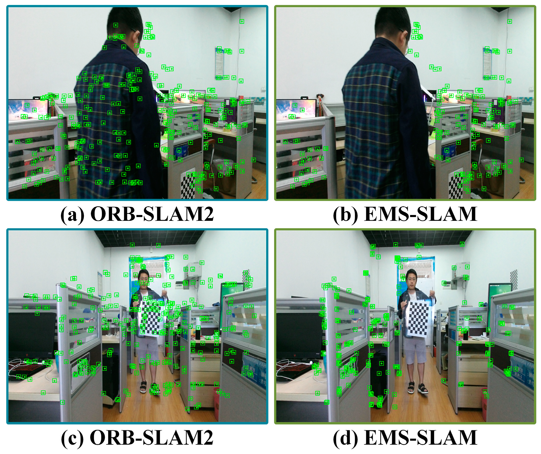
EMS-SLAM was tested on the dynamic scene data collected with a Kinect v2 camera to validate its performance in complex dynamic scenarios. The data, collected in a laboratory setting with people walking, included two dynamic environments named sdjz_w_static_01 and sdjz_w_static_02. The datasets contained color and depth images at a resolution of 640 × 480. The trajectories of the EMS-SLAM and ORB-SLAM2 were evaluated by keeping the Kinect v2 stationary while collecting data. As a result, the Kinect v2 sensor’s actual trajectory was a fixed point in space, and the error was computed as the distance between its estimated and actual trajectory.
The extraction of feature points for the various sequences presented in
Figure 8 was performed for the two different systems: ORB-SLAM2 and EMS-SLAM. Compared with ORB-SLAM2, EMS-SLAM effectively removed all feature points on dynamic objects. As shown in
Table 9, the RMSE accuracy of the ATE improved by 94.45% and 96.25% for the sdjz_w_static_01 and sdjz_w_static_02 sequences, respectively.
3.5. Timing Analysis
The performance of EMS-SLAM was compared with that of other systems by measuring the average time it took for each frame on the TUM dataset, as shown in
Table 10. Systems such as DS-SLAM, YS-SLA [
38], and RDS-SLAM utilize pixel-level semantic segmentation networks, significantly increasing their average frame processing time. While YOLO-SLAM employs an object detection algorithm, its real-time performance is limited by hardware constraints. In contrast, EMS-SLAM uses a lightweight object detection network, greatly enhancing the inference efficiency and processing speed on resource-constrained devices. The average frame processing time for EMS-SLAM increased by only 6.22 milliseconds compared with ORB-SLAM2, fully satisfying the real-time performance requirements of SLAM.
4. Discussion
The EMS-SLAM algorithm proposed in this paper has made significant progress in the field of real-time SLAM, particularly in dynamic environments. By integrating a feature matching method based on GC-RANSAC, we enhanced the initial camera pose estimation, which is crucial for achieving accurate localization in complex scenarios. Additionally, our degeneracy-resistant geometric constraint method, which combines epipolar constraints with multi-view geometric constraints, further strengthens the robustness of the algorithm, addressing common limitations faced by traditional SLAM methods. The inclusion of a parallel object detection thread ensures that the system can handle dynamic objects in real-time, making it suitable for a wide range of practical applications.
However, during the experiments, we observed that the performance of EMS-SLAM may be compromised when images are blurred, particularly in the extraction of semantic information. This issue is particularly pronounced when the camera experiences significant motion or operates in low-light conditions, both of which are common challenges in real-world applications. In these scenarios, feature extraction and matching become unreliable, potentially leading to reduced accuracy in the final pose estimation.
Future improvements will focus on addressing this limitation by enhancing the semantic information extraction process. This could involve integrating more advanced image processing techniques, such as deep learning-based feature extraction methods, which are better equipped to handle blurry or low-quality images.

 ,
, 


