Abstract
Reliable forecasts of large-scale chlorophyll-a (Chl-a) levels one week ahead in the Murray–Darling Basin are essential for water resources management, as increasing Chl-a levels in water bodies indicate possible harmful algal blooms, a serious threat for freshwater security. A lack of high-resolution data in space and time is a major constraint for delivering early warnings. To address data scarcity, we developed a forecasting model integrating remote sensing data and time-series modelling. Using in situ Chl-a measurements from Murray–Darling Basin water bodies, we locally recalibrated a two-band ratio algorithm, namely the Normalized Difference Chlorophyll Index (NDCI), from Sentinel-2 data to derive Chl-a levels. The recalibrated model significantly improved the accuracy of high Chl-a estimates in our dataset after mitigating data heteroscedasticity. Building on these improved satellite-derived Chl-a estimates, we developed a time-series model for forecasting weekly Chl-a levels including quantification of forecast uncertainty through prediction intervals. The developed model, validated at eight sites for 2021–2022 data, performed well at shorter lead times, showing R2 = 0.41 and RMSE = 8.1 μg/L for overall performance at a one-week lead time. The prediction intervals generally aligned well with nominal levels, demonstrating their reliability. This study provides a valuable tool for the water managers/decision-makers to issue early warnings of algal blooms in the Murray–Darling Basin.
1. Introduction
The Murray–Darling Basin is the largest and most complex river system in Australia, providing a multitude of ecosystem services [1,2]. Covering 14% of mainland Australia’s area, it supports over 2.4 million residents [3], including the provision of drinking water. The basin also sustains a rich biodiversity of plant and animal species [4] and serves as a crucial water source for irrigation, fisheries, and recreational activities [5,6,7].
Ensuring good water quality in the basin is essential for these functions, prompting a long-term water quality monitoring program initiated in 1978 across multiple sites on the Murray River and its tributaries [8]. Regular monitoring of blue-green algae (BGA) is a critical component of this program, attracting significant interest from various stakeholders [9]. Prior to 2000, BGA blooms in the Murray River were relatively rare. However, they have become increasingly common in recent years, with extensive blooms recorded in 2009, 2010, 2016, and 2021 [10] covering hundreds of river kilometres over several weeks to months [11]. Some BGA species produce toxins, rendering affected water unsafe for drinking, swimming, and boating. These toxins can also poison wildlife, livestock, and pets, posing significant challenges to the basin communities, farmers, and the tourism industry. Effective water management necessitates reducing and mitigating the risk of BGA events.
Chlorophyll-a (Chl-a), a proxy for algal biomass concentration, is a standard water quality parameter measured in various inland and coastal waters worldwide. Chl-a is a green pigment found in plants and algae that facilitates the conversion of light into energy through photosynthesis [12]. Measuring Chl-a is a cost-effective alternative to estimating phytoplankton abundance and biomass through cell counts [13], which require labour-intensive laboratory analysis. Increasing Chl-a levels typically signal excessive algal growth and the potential of a harmful algal bloom [14]. The purpose of this study is to forecast the large-scale Chl-a concentration one week ahead in the Murray–Darling Basin for water management so that one can issue early warnings and implement timely interventions.
In recent times, various models have been developed to forecast Chl-a levels in water bodies. Some models are physics-based, integrating physical, chemical, and biological processes at an ecosystem scale and describing the spatio-temporal dynamics of Chl-a through complex simulations [15,16,17]. Other models are data-driven, using empirical relationships between Chl-a and a set of predictor variables. Several statistical and machine learning data-driven models have also been applied for forecasting Chl-a, including autoregressive integrated moving average (ARIMA) [18], wavelet neural network [19], wavelet-based fuzzy model [20], wavelet nonlinear autoregressive network [21], artificial neural networks [22], wavelet transform with artificial neural network [23], random forest [24], and support vector regression [25]. With advancements in computational power, neural network-based deep learning approaches, such as Long Short-Term Memory (LSTM) networks, have gained increasing attention for forecasting Chl-a [26,27,28,29,30,31].
Data scarcity has been a primary challenge in forecasting Chl-a concentrations in the Murray–Darling Basin. In situ Chl-a measurements require collecting grab samples in the field in accordance with standard methods and analysing them in the laboratory. While this method is well recognized and widely applied, lab-based Chl-a measurements are labour-intensive and time-consuming, limiting them to periodic intervals and important but limited spots [32,33,34]. In situ Chl-a measurements in the Murray–Darling River systems are only available at most weekly and at less than 20 sites (see Section 2 for more details). Recently, a few optical sensors have been deployed for continuously monitoring Chl-a levels in the Murray–Darling River systems, although there may be a potential loss of accuracy [35,36]. Nevertheless, in situ Chl-a measurements (lab-based or sensor-based) do not allow researchers to map Chl-a concentrations on a large spatial scale and use them directly for forecasting Chl-a beyond localised sampling sites.
Remote sensing has emerged as an effective tool for large-scale Chl-a estimation in various aquatic environments. As Chl-a has distinct absorption and reflection properties in the visible spectrum, particularly in the blue and red wavelengths [37,38], space-borne remote sensing technology can relate the spectral water-leaving signal from the water surface to Chl-a levels. Since the 1970s, research has been undertaken to develop algorithms to estimate Chl-a levels from remote sensing data for different optical types of waters (see, for example, [39] for a comprehensive review). The basic principle of these algorithms is to build a strong linkage between the reflectance of sensitive bands and the Chl-a concentrations in water. One of the most used algorithms, also known as “band algorithms” or “index algorithms”, estimates the Chl-a directly from a combination of remote sensing reflectance bands [37,40,41,42,43,44]. However, the spatial heterogeneity of the optical properties and Chl-a concentrations of the waters makes these algorithms hard to apply universally. Further, the often empirical nature of the algorithms’ parameterizations necessitates that regional tuning should be evaluated in water bodies where they have not been previously applied [45].
Many previous studies on remote sensing estimation of Chl-a concentrations have focused on large-scale open waters, such as oceans, coastal seas, or relatively static inland water bodies like lakes, dams, and reservoirs. Few studies have explored the application of these methods or algorithms to flowing rivers [46], including the Murray–Darling River systems. River channels can be relatively narrow and may cover only a few pixels in commonly used satellite imagery, such as Sentinel-2, which can lead to greater uncertainty.
This study develops an algorithm to forecast large-scale Chl-a concentrations in the Murray–Darling River systems using remote sensing data. Two key technical contributions of this work bridge the gap in current Chl-a forecasting methods: (1) In situ Chl-a measurements were related to remote sensing data along the river centreline, and an “index algorithm” was recalibrated locally for Chl-a retrieval. (2) A time-series forecasting model was built on satellite-derived Chl-a estimates, and forecast uncertainty was quantified to provide more information for decision-making. Our methodology integrates recalibrated NDCI-based Chl-a estimation from Sentinel-2 data with SARIMA time-series forecasting. This approach offers several advantages: it leverages high-resolution satellite data for large-scale Chl-a monitoring, improves accuracy for high Chl-a events through local recalibration, and provides uncertainty quantification via prediction intervals, aiding decision-making. However, it has limitations, including dependence on satellite data quality (e.g., cloud cover), potential overestimation of low Chl-a levels due to NDCI model constraints, and reduced forecast accuracy at longer lead times or for stations with sparse data. The manuscript is organized as follows: Section 2 describes the study area and data; Section 3 outlines a practical method to preprocess remote sensing data and describes the forecasting model and corresponding uncertainty estimation; Section 4 presents the main results; and the paper ends with a discussion and conclusion.
2. Materials and Methods
2.1. Study Area and Data
The Murray River (2508 km) and the Darling River (1545 km) [47], central to the Murray–Darling Basin (MDB) in southeastern Australia, are the two longest rivers in Australia and flow across low-gradient, semi-arid landscapes. Covering around 1 million km2, the basin includes over twenty major rivers and significant groundwater systems. The Great Dividing Range to the east and southeast in the MDB forms the natural boundary of the basin, contributing the highest rainfall and most runoff. The basin’s average annual rainfall is 460 mm, and the average annual potential evapotranspiration is 1174 mm [48]. The flow rates in this lowland river vary significantly within and between years with flow velocities mostly in the range of [0.18, 0.5] m/s [49].
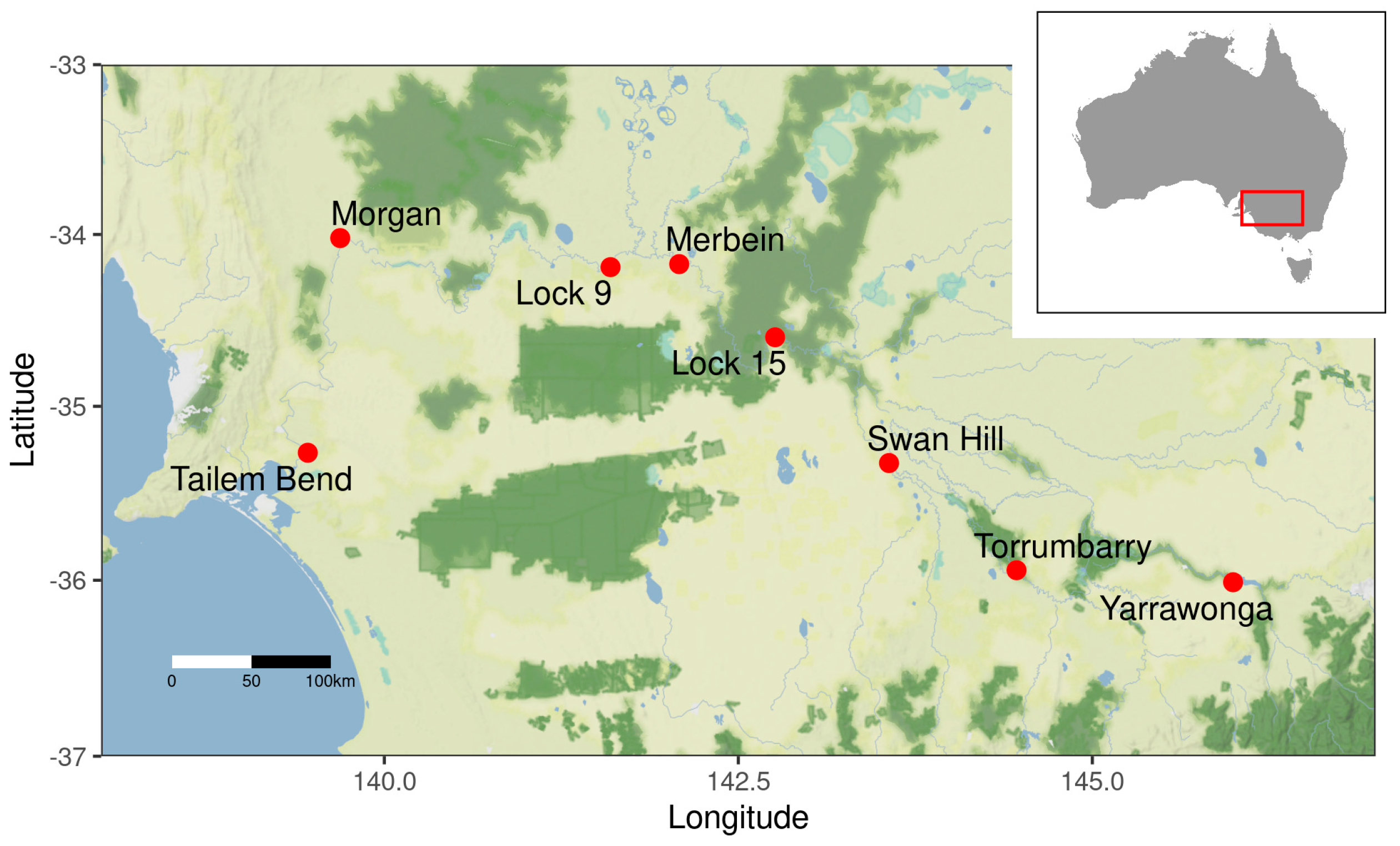
In this study, we used in situ Chl-a measurements from eight sites along the Murray River and its tributaries (Figure 1). These data are the compilation of a long-term water quality monitoring program in the Murray–Darling Basin [10], covering the study period from 2016 to 2022. This study period was chosen because Sentinel-2 imagery, used to derive Chl-a estimates and predictions, has been available since 2016, and in situ Chl-a measurements were available through the end of 2022. The selection criteria for these sites are as follows: (1) each site must have at least 90 in situ Chl-a measurements taken between 2016 and 2022, ensuring sufficient data for analysis; (2) sites located on lakes, such as the Milang Jetty site at Lake Alexandrina, were excluded to focus exclusively on the Murray River. All in situ measurements were collected weekly, though the specific day of collection varied for each sample.
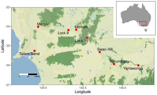
Figure 1.
Location of selected water quality stations in Murray–Darling Basin (Australia Map inside).
The remote sensing data utilized in this study consist of Sentinel-2 MultiSpectral Instrument (MSI) images, developed by the European Space Agency’s (ESA) Sentinel Data Center [50]. Sentinel-2 includes two polar-orbiting satellites, 2A (launched in June 2015) and 2B (launched in March 2017). The Sentinel-2 MSI data comprise 13 wavelength bands, ranging from visible and near-infrared to short-wave infrared, with spatial resolutions of 10 m, 20 m, and 50 m for different bands. Sentinel-2 MSI data have been widely used in various applications to estimate Chl-a levels in water bodies [51,52,53]. We obtained Sentinel-2A/B MSI Analysis Ready Data (Collection 3) from the Digital Earth Australia (DEA) platform, managed by Geoscience Australia [54,55]. This dataset includes validated, calibrated, and adjusted Sentinel-2A/B imagery tailored for Australian conditions, making it ready for analysis. These data are corrected versions of the raw remotely sensed data for atmospheric effects, variations in solar and sensor positions, and surface anisotropic conditions, achieved using Nadir-corrected Bidirectional Reflectance Distribution Function Adjusted Reflectance (NBAR) and terrain illumination adjustments [56]. These corrections ensure consistent, comparable reflectance values across different times, seasons, and locations, enabling accurate surface change detection. To address cloud cover, we applied the Sentinel Hub s2cloudless detector [57] to mask cloud-affected pixels, ensuring data quality. Other factors, such as aerosols or sun glint, were mitigated through DEA’s preprocessing pipeline, though not explicitly filtered.
To develop an algorithm for estimating Chl-a levels from MSI data, we selected “match-up” pairs of in situ measurements and concurrent MSI data based on specific spatial and temporal constraints. For spatial “match-up”, the standard approach for open water bodies (such as lakes and coastal waters) involves selecting a 3 × 3 grid of satellite pixels centred around the sampling location and taking the median value [58]. However, this method is not suitable for the Murray–Darling River systems for the following reasons: (1) many river sections are relatively narrow, and some of the selected 3 × 3 satellite pixels may include land rather than water; (2) sampling points are often near the shore and tree canopies can obstruct satellite views; (3) near-shore satellite imagery may experience interference by the reflectance from the surrounding riverbeds, such as rocks, sand, and debris, which is difficult to isolate.
To address the challenge of selecting pixels centred around the sampling point, avoid adjacency effects as far as possible, and use unmixed pixels in the analysis, we selected all pixels along the centreline of the river extending 300 m upstream of the sampling point. Given that the width of river channels in the Murray–Darling River systems is approximately 40–50 m [59], the distance from a sampling point to the corresponding satellite pixels is around 20–25 m (equivalent to 2–3 pixels). This study utilized RivWidthCloud [60], a Google Earth Engine tool, to extract river centrelines and widths from Sentinel-2 imagery (10 m resolution). RivWidthCloud applies the water classification algorithm from [61] to create a binary water mask, followed by skeletonization for one-pixel-wide centrelines. Preprocessing mitigates vegetation cover and shadows, minimizing terrain-induced errors without direct Digital Elevation Model (DEM)-based correction.
By assuming that Chl-a within this distance is highly correlated, we matched in situ measurements from near-shore locations with remote sensing measurements from the middle of the river. Large blooms often extend over hundreds of river kilometres, making a ±2-day match-up a reasonable compromise in most cases. However, as the bloom or Chl-a magnitude decreases, the extent is likely to become smaller and patchier. In such instances, this match-up approach may be less effective. This approach aligns with the objective of our study, which focuses on developing a forecasting model for Chl-a levels at a large spatial scale instead of a point scale. Given that the selected bands have a 10 m resolution, this initially results in at least 30 satellite pixels. Figure 2 illustrates an example of selected Sentinel 2A/B pixels for Yarrawonga. Further quality control is applied to remove cloudy pixels using cloud masks [57] and non-water pixels using the Modified Normalized Difference Water Index (MNDWI) [62]. The number of remaining valid pixels must be at least 9. Sentinel-2A/B satellites generally have a revisiting period of 5 days. This leads to a total of 850 Sentinel-2A/B images available for the study period (2016–2022). The number of MSI data points is significantly reduced from a maximum of 850 after quality control, as shown in Table 1 for each station. These MSI data formed the basis for estimating and forecasting Chl-a levels at the selected stations in this study. For temporal “match-up”, a window of 2 days between satellite overpass and in situ measurement sampling time was used. In the literature, match-up time windows are commonly a few hours (e.g., 3 or 6 h) [58,63,64] but some studies have chosen longer windows, up to 12 days, for large, stable water bodies [65]. The 2-day window in this study is a practical choice to balance retaining as many match-up pairs as possible while ensuring the satellite and in situ data remain as simultaneous as possible. After applying these spatial and temporal constraints, we obtained 1331 match-up pairs from the selected 8 stations. The number of match-up pairs at each station varies from 106 (Tailem Bend) to 287 (Lock 9). These match-up data were used to estimate the parameters of forecasting models.
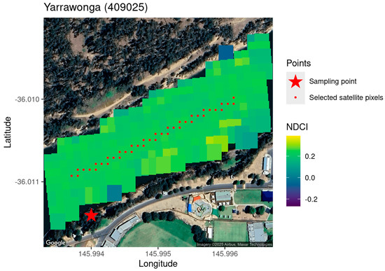
Figure 2.
The NDCI derived from Sentinel-2 imagery on 14 March 2016, for a section of the Murray River near Yarrawonga (409025). Red dots represent the selected pixels used to align with in situ measurements collected at the sampling location, marked by a red star.

Table 1.
Details of water quality stations in Murray River, sorted from upstream to downstream (dataset sizes calculated for period 2016–2022).
2.2. Estimate Chl-a Level from Sentinel MSI Data
To address data scarcity in forecasting Chl-a levels, we estimated Chl-a concentrations from Sentinel MSI data for data augmentation. Specifically, we employed a two-band ratio algorithm based on the Normalized Difference Chlorophyll Index (NDCI) [43] for satellite-derived Chl-a estimates. Originally proposed for use in estuarine and coastal turbid productive waters, the NDCI has been successfully applied to inland freshwater lakes [66,67]. Notably, the NDCI is operationally used for qualitative Chl-a mapping and bloom detection with Sentinel-2 data in Australian waterbodies, including the Murray–Darling River systems, by Geoscience Australia [68].
The NDCI utilizes MSI spectral bands at 705 nm (Band 5) and 665 nm (Band 4), which are highly sensitive to Chl-a absorption and backscattering-induced reflectance, respectively. The NDCI, denoted by , is calculated as the difference in reflectance between these bands, denoted by and , normalized by their sum:
The NDCI has shown a strong relationship with in situ Chl-a measurements in numerous studies [66,67,69,70]. To model the empirical relationship between the NDCI and in situ Chl-a measurements, we used a quadratic function, originally proposed by [43]:
where is the satellite-derived Chl-a estimate at a specific time , and are the parameters in the fitted function. Additionally, an exponential function has been used as an alternative to model the NDCI and Chl-a relationship [71,72]. We tested various alternative functional forms, including higher-order polynomials and exponential functions, to determine the best fit for the relationship. Our analysis indicated that the quadratic function provided a marginally better fit for our data compared to other forms (the results are not included in this manuscript). Consequently, we retained the quadratic function as proposed by [43], but recalibrated the model parameters. Specifically, we refitted the quadratic model with our data (denoted by “recalibrated quadratic model”) and compared it with the original fitted model provided by [43] (denoted by “Mishra quadratic model”).
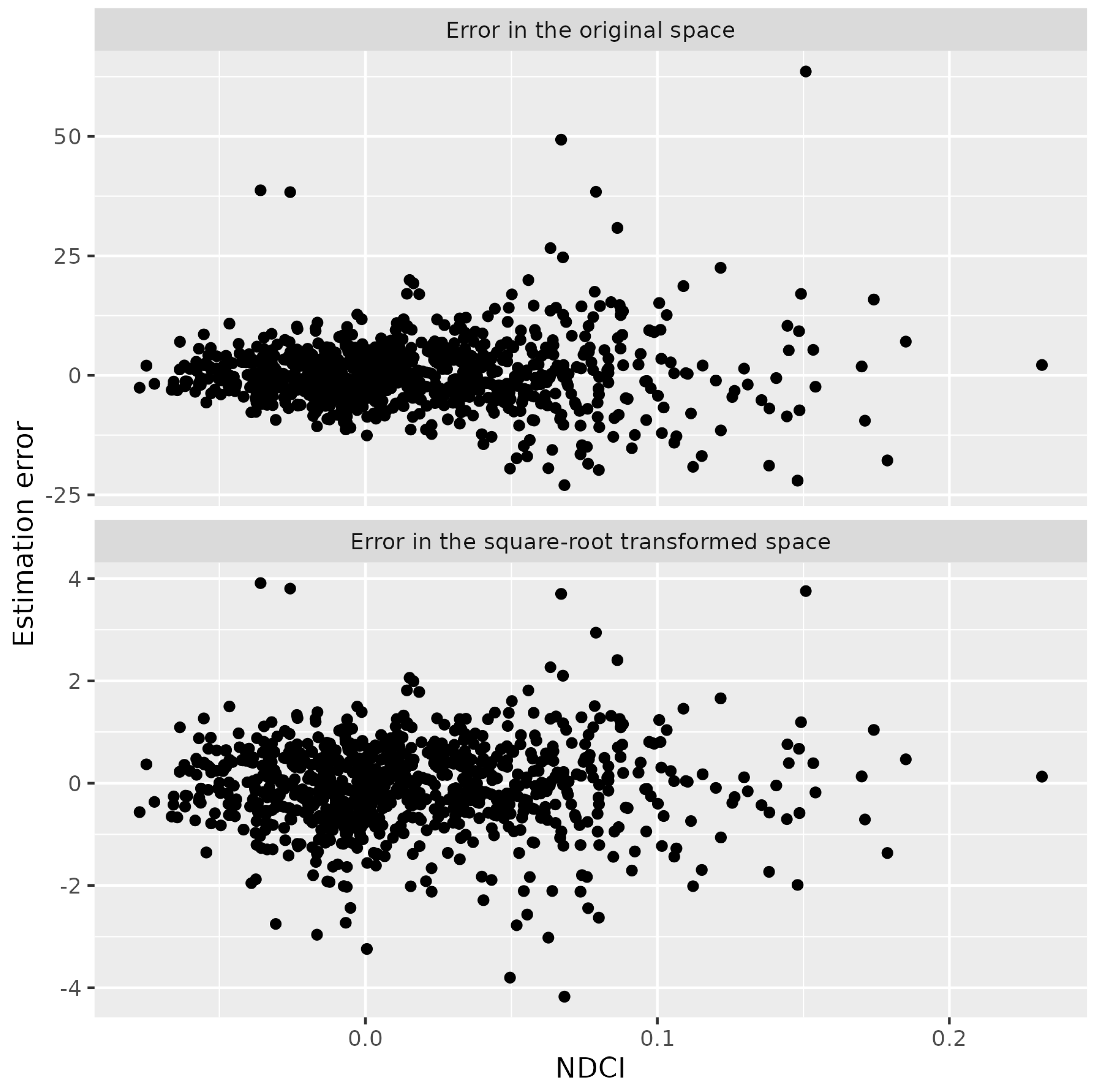
We have observed that the estimation error increases with the NDCI value (Figure 3). To address this heterogeneity for reliable uncertainty quantification, we assumed that the estimation error, after applying a square-root transformation, follows a normal distribution with constant variance. Specifically, we model this as follows:
where is the in situ Chl-a measurement (ground truth) and is the variance parameter. Comparing the two panels in Figure 3, we can see that the square-root transformation is an effective tool to reduce heterogeneity. In the upper panel of Figure 3, the error range in the original space is from −12.5 to 12.5 when the NDCI is less than 0.05 but suddenly increases to −25 to 25 when the NDCI is above 0.05, indicating clear heteroscedasticity. Conversely, in the lower panel of Figure 3, the error range in the transformed space remains more stable across different NDCI ranges. This suggests that the heteroscedasticity issue is significantly reduced after applying a square-root transformation. Equation (3) can then be used to quantify the uncertainty of the satellite-derived Chl-a estimate in Equation (2) in addition to point estimates. The two-sided prediction interval of the satellite-derived Chl-a estimate can be calculated by
where is the quantile of a standard normal distribution. The parameters and are estimated by maximizing the following likelihood function:
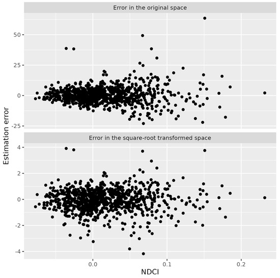
Figure 3.
The error in satellite-derived Chl-a estimates as a function of the NDCI. The top panel shows the estimation error in the original space, while the bottom panel presents the estimation error in the square-root-transformed space (note that the y-axis uses different scales for the top and bottom panels).
2.3. Seasonal Autoregressive Integrated Moving Average Model for Forecasting Chl-a Level from Sentinel MSI Data
We undertook time-series forecasting of the satellite-derived Chl-a levels based on the Box–Jenkins approach [73]. As Chl-a levels exhibit a seasonal pattern, we used the seasonal autoregressive integrated moving average (SARIMA) model to model the weekly time series of satellite-derived Chl-a levels. The SARIMA model is a widely used time-series forecasting tool that extends the classical ARIMA model to accommodate seasonal patterns in data. By combining autoregressive, integrated, and moving average components with seasonal elements, SARIMA provides a robust approach for forecasting time-series data with seasonal fluctuation A based on a time series is given by
where:
- , and are polynomials of the order , and , respectively;
- is the backward shift operator and ;
- is the backward shift operator for the seasonal term and ;
- are the order of integrated and seasonal integrated components;
- is the seasonal period;
- is the white noise error term at time .
To match up the time step of in situ Chl-a measurements, we considered weekly time series of satellite-derived Chl-a. If more than one satellite-derived Chl-a estimate is available in a week, we used the average value to represent the weekly value. As a result, we took the seasonal period parameter as based on the advice from Hyndman [74]. This treatment can overcome the issue that the total number of weeks can be different (either 52 or 53) for different years. The other parameters of the SARIMA model were optimized using the Akaike information criterion (AIC) from the “forecast” [75] package in the R environment. To address the difference in stations, we calibrated the SARIMA model parameters for each station individually.
To quantify forecast uncertainty, we compared the forecast Chl-a levels at time with lead time , denoted by , with the ground truth (i.e., the corresponding in situ measurement ). To identify the increasing forecast uncertainty with an increasing value of , we, similar to in Section 3.1, assumed that the forecast error after a square-root transformation follows a normal distribution and the variance is constant. Similar to Equation (3),
where is the variance parameter for the forecast with lead time and was estimated separately from SARIMA model parameters. Analogous to Equation (4), we can derive the two-sided prediction interval of the Chl-a forecast by
2.4. Model Validation
To test model performance, we divided the entire dataset into two parts: a calibration set from 2016 to 2020 and a validation set from 2021 to 2022. In terms of data volume (i.e., “match-up” pairs of in situ measurements and satellite-derived estimates), the calibration set comprises 67% of the total data, while the validation set comprises 33%. We measured the accuracy of Chl-a point-value forecasts using three validation metrics, the coefficient of determination (R2), the root mean square error (RMSE), and the bias, which are defined below:
R2, also known as Nash–Sutcliffe efficiency in hydrology [76], ranges from negative infinity to 1. An R2 of 1 corresponds to a perfect forecast, where the forecast and in situ Chl-a values are identical at all times. A negative R2 suggests that the mean of historical Chl-a data outperforms the forecasts. RMSE quantifies the magnitude of forecast errors, while forecast bias indicates the direction of these errors. Bias represents the systematic difference between forecast and in situ Chl-a values. An ideal Chl-a forecast is expected to be unbiased. To evaluate the forecast prediction intervals alongside point-value forecasts, we calculated the coverage probability, or simply coverage for short, which is the percentage of in situ Chl-a values that fall within the proposed prediction intervals. The same validation metrics were used to evaluate the performance of satellite-derived Chl-a estimates.
3. Results
3.1. Satellite-Derived Chl-a Estimates
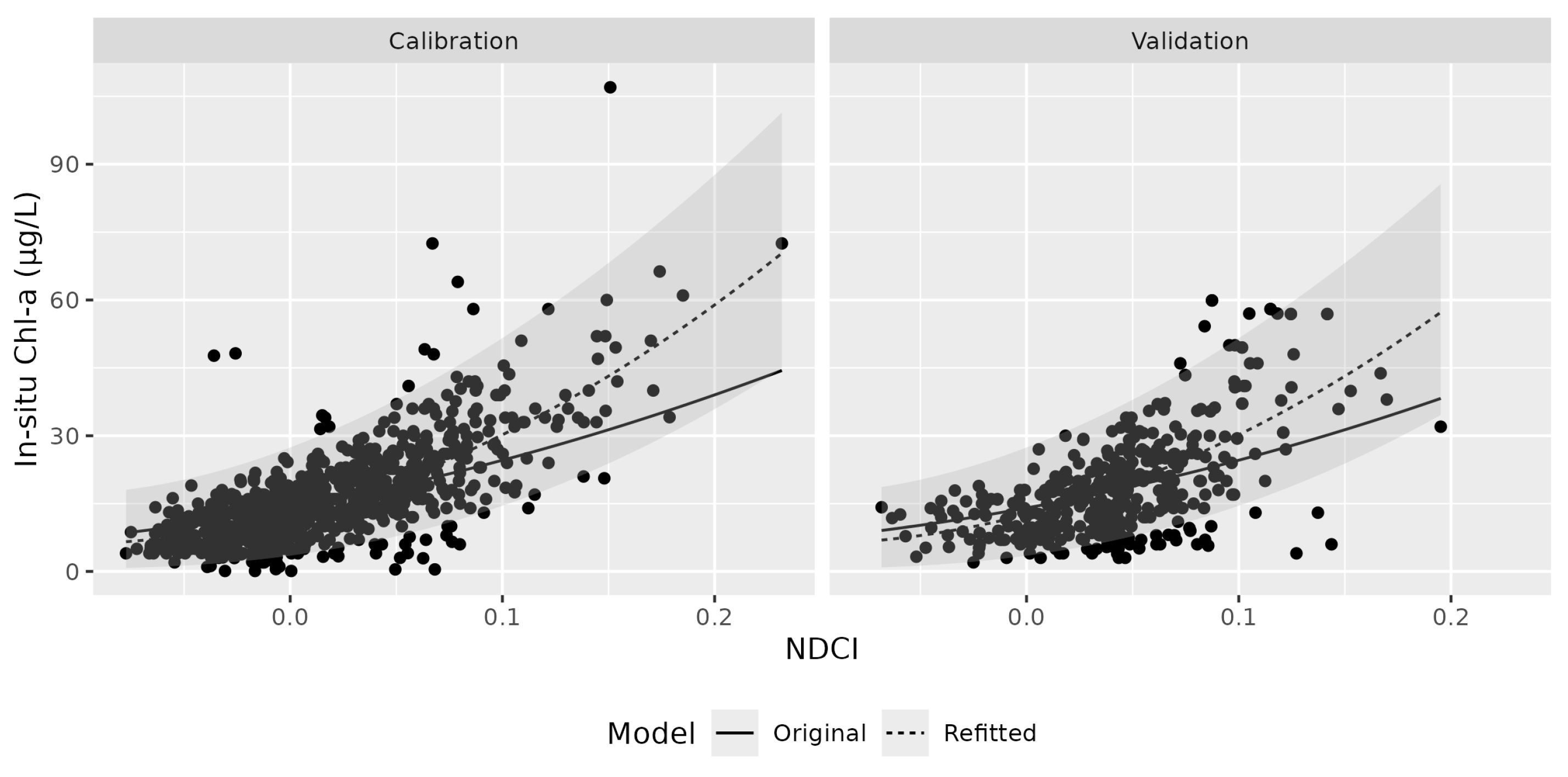
Figure 4 shows the relationship between in situ Chl-a measurements and corresponding NDCI values, as described in Section 3.1. This relationship is an increasing upward concave, a pattern captured by both the original and refitted estimation models (the model parameter values are presented in Table 2). The most notable difference is that the original model is flatter than the refitted one, leading to an underestimation of high Chl-a events, particularly when NDCI values exceed 0.1. The refitted model re-optimizes the parameters based on the calibration data to correct this issue, significantly improving accuracy for high Chl-a events. The 95% prediction intervals for larger NDCI values account for increased estimation error. The patterns observed in the calibration and validation datasets are largely similar, though the goodness-of-fit is slightly better for the calibration data.
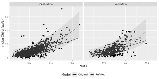
Figure 4.
The relationship between the NDCI and in situ Chl-a is shown with the original model from Mishra and Mishra (2012) (solid line) and the refitted model (dashed line). The shaded area represents the 95% prediction intervals based on the refitted quadratic linear regression. The left and right panels represent the results for the calibration and validation datasets.
Table 2.
The parameter values in the original and refitted model for satellite-derived Chl-a estimates.
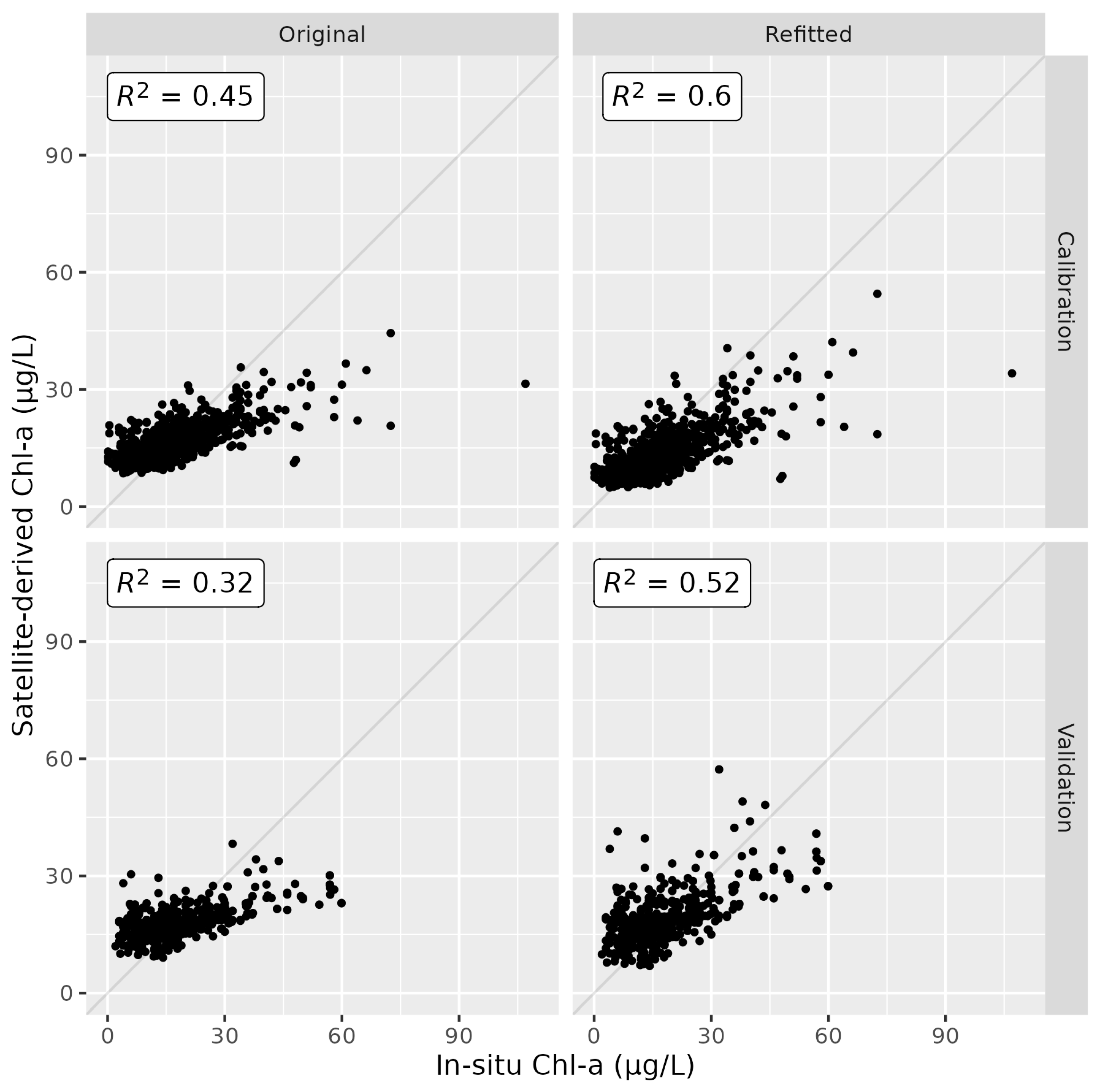
Figure 5 compares the satellite-derived Chl-a estimates with corresponding in situ Chl-a measurements. The original model shows a clear tendency to overestimate low Chl-a events while underestimating high Chl-a events. In contrast, the refitted model mitigates this bias, with scatter points more evenly distributed along the 1:1 line. Nevertheless, there is an outlier where an extremely high Chl-a event was recorded, with an in situ measurement of 107 μg/L on 14 January 2019, at the Lock 9 station. Both models significantly underestimate this event by approximately half. This underestimation may be due to the spatial patchiness of Chl-a, which is not always captured by satellite imagery, especially when the satellite’s overpass time is near the boundary of the ±2-day window from the sampling time, as was the case here.
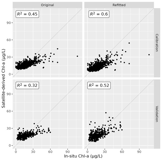
Figure 5.
A comparison of in situ Chl-a measurements and the corresponding satellite-derived Chl-a estimates for the original (left) and refitted (right) quadratic linear regression models based on the calibration (upper) and validation (lower) datasets.
Table 3 supplements Figure 5 by comparing key validation metrics for the two models. The refitted model achieves a higher R2 and lower RMSE than the original model, confirming its overall superior performance. While the original model exhibits slightly less bias for the calibration data, this advantage does not extend to the validation data. Since the primary goal of this study is to effectively forecast algae blooms, we are particularly focused on the model’s performance in predicting high Chl-a events. We adopt a threshold of 30 μg/L, following several studies [77,78,79] that define rivers with Chl-a levels above 30 μg/L as eutrophic. Notably, when focusing on high Chl-a events, the refitted model demonstrates significantly a lower bias and RMSE. This better performance of the refitted model over the original model is consistent for both calibration and validation data. Table 4 presents the coverage of the prediction intervals based on the satellite-derived Chl-a estimate. The observed coverage is close to the nominal levels of 90% and 95%.
Table 3.
Error statistics for original and refitted satellite-derived Chl-a estimates in calibration and validation datasets. For example, R2 is 0.32 for validating original satellite-derived Chl-a estimates.
Table 4.
Error statistics for two satellite-derived Chl-a estimates (original and refitted quadratic linear regression).
3.2. Chl-a Forecasts
Figure 6 presents various error statistics for Chl-a forecasts with lead times ranging from 1 to 4 weeks. The first column of Figure 6 shows the overall performance, calculated by pooling data from all stations. As expected, the overall forecast performance generally deteriorates with increasing lead time, as indicated by the worsening of all error statistics. This trend reflects the intrinsic increase in uncertainty for Chl-a levels as the lead time extends. Compared with the Chl-a estimation statistics (validation data) in Table 3, the overall forecast performance is limited by the accuracy of the satellite-derived Chl-a estimates. Nonetheless, the R2 value remains positive even at a lead time of four weeks, suggesting that the Chl-a forecasts outperform a naïve forecast based on the long-term average. The overall RMSE ranges from 8.1 μg/L at a 1-week lead time to 10.3 μg/L at 4 weeks. The RMSE for high Chl-a events is nearly double that of the overall RMSE. The trend of overall bias increases only slightly with longer lead times, but the negative bias for high Chl-a events becomes more pronounced.
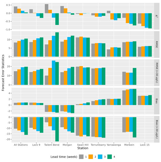
Figure 6.
Forecast error statistics of the proposed Chl-a forecasts as a function of lead time (ranging from 1 to 4 weeks, labelled by different colours) for all stations combined (leftmost column) and each individual station (subsequent columns).
The second to ninth columns of Figure 6 display station-wise forecast performance, which varies across stations. At four stations (Lock 9, Tailem Bend, Morgan, and Yarrawonga), the forecasts yield positive R2 values at shorter lead times (e.g., 0.44 at Morgan for 1-week lead time), indicating reasonable accuracy. Conversely, the other four stations (Swan Hill, Torrumbarry, Merbein, and Lock 15) exhibit negative R2 values across all lead times (e.g., −0.64 at Lock 15 for 1-week lead time), suggesting that forecasts underperform compared to the simple average of the validation data. This performance variation is mainly caused by two key factors: (1) Inaccurate satellite-derived Chl-a estimates compromise SARIMA model performance, particularly at Yarrawonga and Lock 15, where most in situ Chl-a measurements are below 30 μg/L, often under 10 μg/L. For instance, the RMSE at Lock 15 reaches 12.5 μg/L at a 1-week lead time. NDCI-based estimates tend to overestimate low Chl-a levels, exacerbated by our quadratic model’s natural lower bound. (2) The SARIMA model assumes time-series persistence, which may not hold at stations influenced by upstream biomass transport, a factor not included in our model. Future studies could explore incorporating upstream or tributary Chl-a levels to improve forecast accuracy.
Table 4 shows that the observed coverage values of the prediction intervals are generally close to the nominal levels but slightly lower (e.g., 86.2% vs. 90% at 1-week lead time), indicating that the forecast prediction intervals perform well overall but are conservative. For high-Chl-a events (>30 μg/L), coverage drops (e.g., 85% at 2-week lead time), indicating narrower intervals for sporadic peaks. Coverage improves at longer lead times (e.g., 92.8% at 4-week lead time), reflecting wider intervals that better capture variability.
Figure 7 and Figure 8 present the time series of 1-week-ahead Chl-a forecasts for Morgan and Lock 15, representing strong and weak performance, respectively (see Supplementary Materials for other stations). The first example is Morgan (Figure 7), where the 1-week-ahead Chl-a forecast has an R2 of 0.44 (as shown in Figure 5). The Chl-a forecast is highly accurate for 2021, effectively capturing the high peak of 40 μg/L in August 2021. However, the forecast for 2022 is generally less accurate in terms of missing smaller fluctuations (<15 μg/L), possibly due to more random variations in Chl-a levels, which pose a greater challenge for time-series forecasting. The forecast prediction intervals are reasonable, with most in situ measurements falling within them. Figure 7 also shows that the satellite-derived Chl-a estimates provide a good approximation during the calibration period, and the prediction intervals based on these estimates have good coverage. We also note that the prediction interval width for satellite-derived Chl-a estimates is a little bit narrower than that for the Chl-a forecast. The second example is Lock 15 (Figure 8), where the 1-week-ahead Chl-a forecast has an R2 of 0.64 (as shown in Figure 4). The primary issue here is that the algorithm does not predict any values below 10 μg/L, with a mean bias of 8 μg/L, due to the NDCI’s lower-bound issue. Despite this limitation, the proposed forecast algorithm remains effective in providing timely warnings for algal blooms related to high Chl-a events (>30 μg/L), which are of greater importance for decision-making.
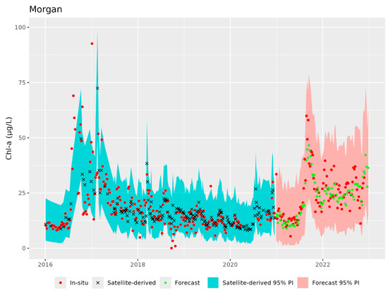
Figure 7.
Time series of Chl-a levels at Morgan. Satellite-derived estimates and corresponding 95% prediction intervals (PI) are used for calibration period (before 1 January 2021) and 1-week ahead Chl-a forecasts are used for validation period (from 1 January 2021).
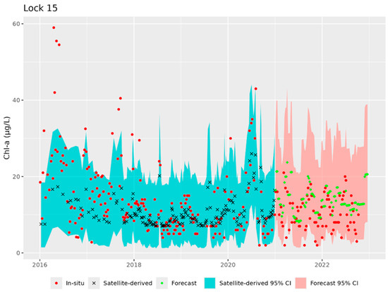
Figure 8.
Time series of Chl-a levels at Lock 15. Satellite-derived estimates and corresponding 95% prediction intervals are used for calibration period (before 1 January 2021) and Chl-a forecasts are used for validation period (from 1 January 2021).
4. Discussion
Cyanobacterial harmful algal blooms in freshwater can also be measured by the abundance of phycocyanin, a photosynthetic pigment unique to cyanobacteria [80]. In certain circumstances, phycocyanin can be a more specific indicator of cyanobacterial abundance than Chl-a [81]. In this study, Chl-a was chosen as a proxy for algal biomass concentrations primarily for two reasons: (1) Remote sensing measurement of phycocyanin is less common compared to Chl-a, as most operational satellites lack sensor bands that uniquely identify the reflectance signal of phycocyanin [82,83]. (2) There is a lack of phycocyanin data collected in the Murray–Darling River system, making it challenging to test model performance. In the future, advanced remote sensing and more in situ measurements could enable phycocyanin and Chl-a forecasting, improving harmful blue-green algae monitoring in the Murray–Darling Basin.
Achieving accurate inversion of high Chl-a concentrations using satellite imagery alone is challenging. The empirical formula may be affected by local water body optical parameters, increasing errors in satellite-derived Chl-a estimates for high Chl-a levels (Figure 5). Additional information on typical species characteristics and suspended particulates in local water bodies would be beneficial to improve accuracy for high Chl-a levels. Similarly, the NDCI algorithm’s natural lower-bound issue causes overestimation of low Chl-a concentrations (<10 μg/L), as seen at Lock 15 (Figure 8), reducing forecast accuracy at low Chl-a sites. Segmented modelling, using distinct NDCI calibrations for low and high Chl-a ranges, could mitigate low-Chl-a bias. However, this study is limited by the availability of data, as no other optically active parameters were available for the local water bodies beyond Chl-a levels. The prediction intervals, as a measure of estimation uncertainty, reflect the high uncertainty for high and low Chl-a levels and are considered a good complement to point estimates for better decision-making. Although the actual Chl-a concentrations may be subject to errors, identifying rapidly changing trends or changes in relative quantity can still serve as good indicators for algal blooms.
Algal blooms are generally more likely to occur when temperatures and radiation rise, such as during summer, but seasonality is not the primary cause of algal blooms in the Murray–Darling River systems, and distinct seasonal patterns are not observed in the study region. For example, a significant algal bloom event in 2016 occurred in the Murray River system, stretching across 2360 km of river length, lasting from February (summer) to June (winter) [11]. Therefore, training the empirical inversion formula separately for different seasons may be effective in improving accuracy. A broader training dataset could improve satellite Chl-a estimation accuracy, especially for underrepresented high-Chl-a events. Finally, it is important to emphasize that the empirical inversion formula calibrated in this study may not be accurate for other freshwater river systems, as optical properties can vary significantly between river systems. Further validation and calibration are required for implementation in other regions.
ARIMA models were applied for time-series forecasting primarily due to the limited available data for training. Forecasting models need to be calibrated for each site individually to account for site-specific characteristics, resulting in relatively small training datasets for each site (see Table 1). ARIMA models generally perform more stably with small sample sizes compared to deep learning-based models such as LSTM [26] or LSTM combined with random forest [28]. In the literature, these deep learning-based models generally require more than 1000 samples for model training. In the future, it is promising to extend this work with more sophisticated forecasting models as more in situ measurements become available.
5. Conclusions
There is an increasing need from water resources managers and water utilities for real-time monitoring and forecasting of harmful algal blooms in times of climate change. Many of the blooms can be toxin-producing, threatening limited freshwater resources. This study demonstrates the effectiveness of forecasting Chl-a levels based on satellite-derived Chl-a estimates for the Murray–Darling River systems. We achieved an improved accuracy over classical Chl-a estimates based on the NDCI by refitting the model with measurements from local grab samples. Hence, the Chl-a forecasting model developed is based on the improved satellite-derived Chl-a estimates, providing useful point forecasts as well as prediction intervals. The point measurements based Chl-a forecast perform well at shorter lead times and show positive R2 values for overall forecast performance up to four weeks, although performance varies across stations. Prediction intervals for these forecasts generally work well and align with nominal levels, though they may be sometimes narrow for sporadic extremely high-Chl-a events. Therefore, we provided some evidence that the proposed Chl-a forecasting model can be used for early warnings of algal blooms in rivers of the Murray–Darling Basin.
Supplementary Materials
The following supporting information can be downloaded at https://www.mdpi.com/article/10.3390/rs17101684/s1.
Author Contributions
Conceptualization, M.L. and K.J.; methodology, M.L.; software, M.L. and L.R.G.; validation, M.L.; formal analysis, M.L.; investigation, M.L, K.J., P.T., T.K.B. and H.J.; resources, P.T. and L.R.G.; data curation, M.L. and K.J.; writing—original draft preparation, M.L.; writing—review and editing, K.J., P.T., L.R.G., T.K.B. and H.J.; supervision, K.J. and P.T.; funding acquisition, K.J. and P.T. All authors have read and agreed to the published version of the manuscript.
Funding
This work was supported by Digital Water and Landscapes and AquaWatch projects from the CSIRO Environment Research Unit.
Data Availability Statement
The Sentinel-2A/B MSI datasets are available from the following source: https://knowledge.dea.ga.gov.au/data/product/dea-surface-reflectance-sentinel-2a-msi/ (accessed on 6 November 2024). Chl-a data are available on request from Australian state agencies (Victoria’s Water Measurement Information System (https://data.water.vic.gov.au/victorias-water-measurement-information-system/) (accessed on 8 May 2025), WaterNSW Waterinsights (https://waterinsights.waternsw.com.au/) (accessed on 8 May 2025), and Water Data SA (https://water.data.sa.gov.au/) (accessed on 8 May 2025).
Acknowledgments
We gratefully acknowledge the constructive comments from the four reviewers and the academic editor which significantly improved the presentation of this manuscript.
Conflicts of Interest
The authors declare no conflicts of interest.
References
- Liu, S.; Crossman, N.D.; Nolan, M.; Ghirmay, H. Bringing ecosystem services into integrated water resources management. J. Environ. Manag. 2013, 129, 92–102. [Google Scholar] [CrossRef]
- MacDonald, D.H.; Bark, R.H.; Coggan, A. Is ecosystem service research used by decision-makers? A case study of the Murray-Darling Basin, Australia. Landsc. Ecol. 2014, 29, 1447–1460. [Google Scholar] [CrossRef]
- MDBA. Why the Murray–Darling Basin Matters. Available online: https://www.mdba.gov.au/basin/why-murray-darling-basin-matters (accessed on 22 July 2024).
- MDBA. Plants and Wildlife. Available online: https://www.mdba.gov.au/basin/plants-and-wildlife (accessed on 20 March 2024).
- Swirepik, J.L.; Burns, I.C.; Dyer, F.J.; Neave, I.A.; O’Brien, M.G.; Pryde, G.M.; Thompson, R.M. Establishing Environmental Water Requirements for the Murray-Darling Basin, Australia’s Largest Developed River System. River Res. Appl. 2016, 32, 1153–1165. [Google Scholar] [CrossRef]
- Beare, S.; Heaney, A. Irrigation, Water Quality and Water Rights in the Murray Darling Basin, Australia. Nat. Res. Manag. Policy 2006, 29, 177–198. [Google Scholar] [CrossRef]
- Grafton, R.Q.; Wheeler, S.A. Economics of Water Recovery in the Murray-Darling Basin, Australia. Annu. Rev. Resour. Econ. 2018, 10, 487–510. [Google Scholar] [CrossRef]
- Biswas, T.; Lawrence, B. Revision of the River Murray Water Quality Monitoring Program; Internal MDBA Report 18/15; 2013; p. 29. Available online: https://www.researchgate.net/publication/323571660_Revision_of_the_River_Murray_Water_Quality_Monitoring_Program?channel=doi&linkId=5a9e0ad6aca272cd09c229f7&showFulltext=true (accessed on 8 May 2025).
- Holland, A.; Gionfriddo, C.; McPhan, L.; Lewis, S.; Shackleton, M.; Silvester, E. Synthesis of Blue Green Algae (Cyanobacteria) Bloom Knowledge and Analysis of Recent Trends in the Murray Darling Basin; 1; La Trobe Biogeochemistry and Ecotoxicology Group: 2023. Available online: https://www.mdba.gov.au/sites/default/files/publications/synthesis-blue-green-algae-bloom-knowledge-analysis-recent-trends-mdb.pdf (accessed on 8 May 2025).
- Biswas, T.; Mosley, L.M. From Mountain Ranges to Sweeping Plains, in Droughts and Flooding Rains; River Murray Water Quality over the Last Four Decades. Water Resour. Manag. 2019, 33, 1087–1101. [Google Scholar] [CrossRef]
- Bowling, L.; Baldwin, D.; Merrick, C.; Brayan, J.; Panther, J. Possible drivers of a Chrysosporum ovalisporum bloom in the Murray River, Australia, in 2016. Mar. Freshw. Res. 2018, 69, 1649–1662. [Google Scholar] [CrossRef]
- Krause, G.H.; Weis, E. Chlorophyll Fluorescence and Photosynthesis—The Basics. Annu. Rev. Plant Phys. 1991, 42, 313–349. [Google Scholar] [CrossRef]
- Rowan, K.S. Photosynthetic Pigments of Algae; Cambridge University Press: Cambridge, UK; New York, NY, USA, 1989; p. 334. [Google Scholar]
- Wetzel, R.G. Limnology: Lake and River Ecosystems, 3rd ed.; Academic Press: San Diego, CA, USA, 2001. [Google Scholar]
- Arnold, J.G.; Moriasi, D.N.; Gassman, P.W.; Abbaspour, K.C.; White, M.J.; Srinivasan, R.; Santhi, C.; Harmel, R.D.; van Griensven, A.; Van Liew, M.W.; et al. Swat: Model Use, Calibration, and Validation. Trans. ASABE 2012, 55, 1491–1508. [Google Scholar] [CrossRef]
- Hamilton, D.P.; Schladow, S.G. Prediction of water quality in lakes and reservoirs.1. Model description. Ecol. Model. 1997, 96, 91–110. [Google Scholar] [CrossRef]
- Benndorf, J.; Recknagel, F. Problems of Application of the Ecological Model Salmo to Lakes and Reservoirs Having Various Trophic States. Ecol. Model. 1982, 17, 129–145. [Google Scholar] [CrossRef]
- Chen, Q.W.; Guan, T.S.; Yun, L.; Li, R.N.; Recknagel, F. Online forecasting chlorophyll a concentrations by an auto-regressive integrated moving average model: Feasibilities and potentials. Harmful Algae 2015, 43, 58–65. [Google Scholar] [CrossRef]
- Xiao, X.; He, J.Y.; Huang, H.M.; Miller, T.R.; Christakos, G.; Reichwaldt, E.S.; Ghadouani, A.; Lin, S.P.; Xu, X.H.; Shi, J.Y. A novel single-parameter approach for forecasting algal blooms. Water Res. 2017, 108, 222–231. [Google Scholar] [CrossRef]
- Kim, Y.; Shin, H.S.; Plummer, J.D. A wavelet-based autoregressive fuzzy model for forecasting algal blooms. Environ. Model. Softw. 2014, 62, 1–10. [Google Scholar] [CrossRef]
- Du, Z.H.; Qin, M.J.; Zhang, F.; Liu, R.Y. Multistep-ahead forecasting of chlorophyll a using a wavelet nonlinear autoregressive network. Knowl.-Based Syst. 2018, 160, 61–70. [Google Scholar] [CrossRef]
- Lee, J.H.W.; Huang, Y.; Dickman, M.; Jayawardena, A.W. Neural network modelling of coastal algal blooms. Ecol. Model. 2003, 159, 179–201. [Google Scholar] [CrossRef]
- Kim, M.E.; Shon, T.S.; Shin, H.S. Forecasting algal bloom (chl-a) on the basis of coupled wavelet transform and artificial neural networks at a large lake. Desalin. Water Treat. 2013, 51, 4118–4128. [Google Scholar] [CrossRef]
- Yajima, H.; Derot, J. Application of the Random Forest model for chlorophyll-a forecasts in fresh and brackish water bodies in Japan, using multivariate long-term databases. J. Hydroinform 2018, 20, 206–220. [Google Scholar] [CrossRef]
- Rajaee, T.; Boroumand, A. Forecasting of chlorophyll-a concentrations in South San Francisco Bay using five different models. Appl. Ocean. Res. 2015, 53, 208–217. [Google Scholar] [CrossRef]
- Abbas, A.; Park, M.; Baek, S.S.; Cho, K.H. Deep learning-based algorithms for long-term prediction of chlorophyll-a in catchment streams. J. Hydrol. 2023, 626, 130240. [Google Scholar] [CrossRef]
- Yao, L.L.; Wang, X.P.; Zhang, J.H.; Yu, X.; Zhang, S.C.; Li, Q. Prediction of Sea Surface Chlorophyll-a Concentrations Based on Deep Learning and Time-Series Remote Sensing Data. Remote Sens. 2023, 15, 4486. [Google Scholar] [CrossRef]
- Cen, H.B.; Jiang, J.H.; Han, G.Q.; Lin, X.Y.; Liu, Y.; Jia, X.Y.; Ji, Q.Y.; Li, B. Applying Deep Learning in the Prediction of Chlorophyll-a in the East China Sea. Remote Sens. 2022, 14, 5461. [Google Scholar] [CrossRef]
- Shin, Y.; Kim, T.; Hong, S.; Lee, S.; Lee, E.; Hong, S.; Lee, C.; Kim, T.; Park, M.S.; Park, J.; et al. Prediction of Chlorophyll-a Concentrations in the Nakdong River Using Machine Learning Methods. Water 2020, 12, 1822. [Google Scholar] [CrossRef]
- Liu, N.; Chen, S.Y.; Cheng, Z.Y.; Wang, X.; Xiao, Y.; Xiao, L.; Gong, Y.W.; Wang, T.T.; Zhang, X.F.; Liu, S.Q. Long-term prediction of sea surface chlorophyll-a concentration based on the combination of spatio-temporal features. Water Res. 2022, 211, 118040. [Google Scholar] [CrossRef]
- Chen, C.; Chen, Q.W.; Yao, S.Y.; He, M.N.; Zhang, J.Y.; Li, G.; Lin, Y.Q. Combining physical-based model and machine learning to forecast chlorophyll-a concentration in freshwater lakes. Sci. Total Environ. 2024, 907, 168097. [Google Scholar] [CrossRef] [PubMed]
- An, Y.J.; Kampbell, D.H. Monitoring chlorophyll-a as a measure of algae in Lake Texoma marinas. Bull. Environ. Contam. Toxicol. 2003, 70, 606–611. [Google Scholar] [CrossRef]
- Davies, C.H.; Ajani, P.; Armbrecht, L.; Atkins, N.; Baird, M.E.; Beard, J.; Bonham, P.; Burford, M.; Clementson, L.; Coad, P.; et al. A database of chlorophyll a in Australian waters. Sci. Data 2018, 5, 180018. [Google Scholar] [CrossRef]
- Filazzola, A.; Mahdiyan, O.; Shuvo, A.; Ewins, C.; Moslenko, L.; Sadid, T.; Blagrave, K.; Imrit, M.A.; Gray, D.K.; Quinlan, R.; et al. A database of chlorophyll and water chemistry in freshwater lakes. Sci. Data 2020, 7, 310. [Google Scholar] [CrossRef] [PubMed]
- Chowdhury, R.I.; Wahid, K.A.; Nugent, K.; Baulch, H. Design and Development of Low-Cost, Portable, and Smart Chlorophyll-A Sensor. IEEE Sens. J. 2020, 20, 7362–7371. [Google Scholar] [CrossRef]
- Zeng, L.H.; Li, D.L. Development of Sensors for Chlorophyll Concentration Measurement. J. Sens. 2015, 2015, 903509. [Google Scholar] [CrossRef]
- O’Reilly, J.E.; Werdell, P.J. Chlorophyll algorithms for ocean color sensors-OC4, OC5 & OC6. Remote Sens. Environ. 2019, 229, 32–47. [Google Scholar] [CrossRef]
- Gitelson, A. The Peak near 700 Nm on Radiance Spectra of Algae and Water—Relationships of Its Magnitude and Position with Chlorophyll Concentration. Int. J. Remote Sens. 1992, 13, 3367–3373. [Google Scholar] [CrossRef]
- Gholizadeh, M.H.; Melesse, A.M.; Reddi, L. A Comprehensive Review on Water Quality Parameters Estimation Using Remote Sensing Techniques. Sensors 2016, 16, 1298. [Google Scholar] [CrossRef] [PubMed]
- Hu, C.M.; Lee, Z.; Franz, B. Chlorophyll a algorithms for oligotrophic oceans: A novel approach based on three-band reflectance difference. J. Geophys. Res.-Ocean. 2012, 117, C01011. [Google Scholar] [CrossRef]
- Moses, W.J.; Gitelson, A.A.; Berdnikov, S.; Saprygin, V.; Povazhnyi, V. Operational MERIS-based NIR-red algorithms for estimating chlorophyll-a concentrations in coastal waters—The Azov Sea case study. Remote Sens. Environ. 2012, 121, 118–124. [Google Scholar] [CrossRef]
- Smith, M.E.; Lain, L.R.; Bernard, S. An optimized Chlorophyll-a switching algorithm for MERIS and OLCI in phytoplankton-dominated waters. Remote Sens. Environ. 2018, 215, 217–227. [Google Scholar] [CrossRef]
- Mishra, S.; Mishra, D.R. Normalized difference chlorophyll index: A novel model for remote estimation of chlorophyll-a concentration in turbid productive waters. Remote Sens. Environ. 2012, 117, 394–406. [Google Scholar] [CrossRef]
- Moses, W.J.; Gitelson, A.A.; Berdnikov, S.; Povazhnyy, V. Satellite estimation of chlorophyll-a concentration using the red and NIR bands of MERIS—The Azov sea case study. IEEE Geosci. Remote Sens. Lett. 2009, 6, 845–849. [Google Scholar] [CrossRef]
- Dogliotti, A.I.; Gossn, J.I.; Gonzalez, C.; Yema, L.; Sanchez, M.; Farrell, I.L.O. Evaluation of Multi- and Hyper- Spectral Chl-A Algorithms in the RÍo De La Plata Turbid Waters During a Cyanobacteria Bloom. In Proceedings of the 2021 IEEE International Geoscience and Remote Sensing Symposium IGARSS, Brussels, Belgium, 11–16 July 2021; pp. 7442–7445. [Google Scholar]
- Ma, Y.X.; Sun, D.Q.; Liu, W.H.; You, Y.F.; Wang, S.Y.; Sun, Z.C.; Wang, S.H. Using a Remote-Sensing-Based Piecewise Retrieval Algorithm to Map Chlorophyll-a Concentration in a Highland River System. Remote Sens. 2022, 14, 6119. [Google Scholar] [CrossRef]
- Geoscience Australia. Longest Rivers. Available online: https://www.ga.gov.au/scientific-topics/national-location-information/landforms/longest-rivers (accessed on 25 September 2024).
- MDBA. Climate—The Murray–Darling Basin. Available online: https://www.mdba.gov.au/climate-and-river-health/climate (accessed on 7 May 2024).
- Mallen-Cooper, M.; Zampatti, B.; Hillman, T.; King, A.; Koehn, J.; Saddlier, S.; Sharpe, C.; Stuart, I. Managing the Chowilla Creek Environmental Regulator for Fish Species at Risk. South Australian Murray-Darling Basin Natural Resources Management Technical Report. 2011. Available online: https://www.researchgate.net/publication/287841440_Managing_the_Chowilla_creek_environmental_regulator_for_fish_species_at_risk?channel=doi&linkId=567a146808ae40c0e27dfa97&showFulltext=true (accessed on 8 May 2025).
- Drusch, M.; Del Bello, U.; Carlier, S.; Colin, O.; Fernandez, V.; Gascon, F.; Hoersch, B.; Isola, C.; Laberinti, P.; Martimort, P.; et al. Sentinel-2: ESA’s Optical High-Resolution Mission for GMES Operational Services. Remote Sens. Environ. 2012, 120, 25–36. [Google Scholar] [CrossRef]
- Gohin, F.; Van der Zande, D.; Tilstone, G.; Eleveld, M.A.; Lefebvre, M.; Andrieux-Loyer, F.; Blauw, A.N.; Bryère, P.; Devreker, D.; Gamesson, P.; et al. Twenty years of satellite and observations of surface chlorophyll-a from the northern Bay of Biscay to the eastern English Channel. Is the water quality improving? Remote Sens. Environ. 2019, 233, 111343. [Google Scholar] [CrossRef]
- Neil, C.; Spyrakos, E.; Hunter, P.D.; Tyler, A.N. A global approach for chlorophyll-a retrieval across optically complex inland waters based on optical water types. Remote Sens. Environ. 2019, 229, 159–178. [Google Scholar] [CrossRef]
- Ogashawara, I.; Kiel, C.; Jechow, A.; Kohnert, K.; Ruhtz, T.; Grossart, H.P.; Hölker, F.; Nejstgaard, J.C.; Berger, S.A.; Wollrab, S. The Use of Sentinel-2 for Chlorophyll-a Spatial Dynamics Assessment: A Comparative Study on Different Lakes in Northern Germany. Remote Sens. 2021, 13, 1542. [Google Scholar] [CrossRef]
- Geoscience Australia. Geoscience Australia Sentinel-2A MSI Analysis Ready Data Collection 3—DEA Surface Reflectance (Sentinel-2A MSI). Available online: https://ecat.ga.gov.au/geonetwork/srv/eng/catalog.search#/metadata/146552 (accessed on 8 May 2024).
- Geoscience Australia. Geoscience Australia Sentinel-2B MSI Analysis Ready Data Collection 3—DEA Surface Reflectance (Sentinel-2B MSI). Available online: https://ecat.ga.gov.au/geonetwork/srv/eng/catalog.search#/metadata/146551 (accessed on 8 May 2024).
- Li, F.Q.; Jupp, D.L.B.; Reddy, S.; Lymburner, L.; Mueller, N.; Tan, P.; Islam, A. An Evaluation of the Use of Atmospheric and BRDF Correction to Standardize Landsat Data. IEEE J.-Stars. 2010, 3, 257–270. [Google Scholar] [CrossRef]
- Skakun, S.; Wevers, J.; Brockmann, C.; Doxani, G.; Aleksandrov, M.; Batic, M.; Frantz, D.; Gascon, F.; Gómez-Chova, L.; Hagolle, O.; et al. Cloud Mask Intercomparison eXercise (CMIX): An evaluation of cloud masking algorithms for Landsat 8 and Sentinel-2. Remote Sens. Environ. 2022, 274, 112990. [Google Scholar] [CrossRef]
- Pahlevan, N.; Smith, B.; Schalles, J.; Binding, C.; Cao, Z.G.; Ma, R.H.; Alikas, K.; Kangro, K.; Gurlin, D.; Hà, N.; et al. Seamless retrievals of chlorophyll-a from Sentinel-2 (MSI) and Sentinel-3 (OLCI) in inland and coastal waters: A machine-learning approach. Remote Sens. Environ. 2020, 240, 111604. [Google Scholar] [CrossRef]
- Victorian Fisheries Authority. The Murray River. Available online: https://vfa.vic.gov.au/recreational-fishing/fishing-locations/inland-angling-guide/special-articles/the-murray-river#:~:text=The%20river%20is%2040%2D50,pools%204%2D5%20m%20deep. (accessed on 31 January 2025).
- Yang, X.; Pavelsky, T.M.; Allen, G.H.; Donchyts, G. RivWidthCloud: An Automated Google Earth Engine Algorithm for River Width Extraction From Remotely Sensed Imagery. IEEE Geosci. Remote Sens. Lett. 2020, 17, 217–221. [Google Scholar] [CrossRef]
- Jones, J.W. Improved Automated Detection of Subpixel-Scale Inundation—Revised Dynamic Surface Water Extent (DSWE) Partial Surface Water Tests. Remote Sens. 2019, 11, 374. [Google Scholar] [CrossRef]
- Xu, H.Q. Modification of normalised difference water index (NDWI) to enhance open water features in remotely sensed imagery. Int. J. Remote Sens. 2006, 27, 3025–3033. [Google Scholar] [CrossRef]
- Cao, Z.G.; Ma, R.H.; Duan, H.T.; Pahlevan, N.; Melack, J.; Shen, M.; Xue, K. A machine learning approach to estimate chlorophyll-a from Landsat-8 measurements in inland lakes. Remote Sens. Environ. 2020, 248, 111974. [Google Scholar] [CrossRef]
- Werther, M.; Odermatt, D.; Simis, S.G.H.; Gurlin, D.; Lehmann, M.K.; Kutser, T.; Gupana, R.; Varley, A.; Hunter, P.D.; Tyler, A.N.; et al. A Bayesian approach for remote sensing of chlorophyll-a and associated retrieval uncertainty in oligotrophic and mesotrophic lakes. Remote Sens. Environ. 2022, 283, 113295. [Google Scholar] [CrossRef]
- Li, S.J.; Song, K.S.; Wang, S.; Liu, G.; Wen, Z.D.; Shang, Y.X.; Lyu, L.L.; Chen, F.F.; Xu, S.Q.; Tao, H.; et al. Quantification of chlorophyll-a in typical lakes across China using Sentinel-2 MSI imagery with machine learning algorithm. Sci. Total Environ. 2021, 778, 146271. [Google Scholar] [CrossRef]
- Zhang, F.F.; Li, J.S.; Shen, Q.; Zhang, B.; Wu, C.Q.; Wu, Y.F.; Wang, G.L.; Wang, S.L.; Lu, Z.Y. Algorithms and Schemes for Chlorophyll a Estimation by Remote Sensing and Optical Classification for Turbid Lake Taihu, China. IEEE J.-Stars. 2015, 8, 350–364. [Google Scholar] [CrossRef]
- Buma, W.G.; Lee, S.I. Evaluation of Sentinel-2 and Landsat 8 Images for Estimating Chlorophyll-a Concentrations in Lake Chad, Africa. Remote Sens. 2020, 12, 2437. [Google Scholar] [CrossRef]
- Geoscience Australia. Monitoring Chlorophyll-a in Australian Waterbodies. Available online: https://knowledge.dea.ga.gov.au/notebooks/Real_world_examples/Chlorophyll_monitoring/ (accessed on 9 August 2024).
- Beck, R.; Zhan, S.G.; Liu, H.X.; Tong, S.; Yang, B.; Xu, M.; Ye, Z.X.; Huang, Y.; Shu, S.; Wu, Q.S.; et al. Comparison of satellite reflectance algorithms for estimating chlorophyll-a in a temperate reservoir using coincident hyperspectral aircraft imagery and dense coincident surface observations. Remote Sens. Environ. 2016, 178, 15–30. [Google Scholar] [CrossRef]
- Mishra, D.R.; Schaeffer, B.A.; Keith, D. Performance evaluation of normalized difference chlorophyll index in northern Gulf of Mexico estuaries using the Hyperspectral Imager for the Coastal Ocean. Gisci Remote Sens. 2014, 51, 175–198. [Google Scholar] [CrossRef]
- Kravitz, J.; Matthews, M. Chlorophyll-a for Cyanobacteria Blooms from Sentinel-2. Available online: https://custom-scripts.sentinel-hub.com/custom-scripts/sentinel-2/cyanobacteria_chla_ndci_l1c/ (accessed on 9 August 2024).
- Manuel, A.; Blanco, A.C. Transformation of the normalized difference chlorophyll index to retrieve chlorophyll-a concentrations in Manila Bay. Int. Arch. Photogramm. Remote Sens. Spat. Inf. Sci. 2023, XLVIII-4/W6-2022, 217–221. [Google Scholar] [CrossRef]
- Makridakis, S.; Hibon, M. ARMA models and the Box-Jenkins methodology. J. Forecast. 1997, 16, 147–163. [Google Scholar] [CrossRef]
- Hyndman, R. Forecasting Weekly Data. Available online: https://robjhyndman.com/hyndsight/forecasting-weekly-data/ (accessed on 19 August 2024).
- Hyndman, R.; Athanasopoulos, G.; Bergmeir, C.; Caceres, G.; Chhay, L.; O’Hara-Wild, M.; Petropoulos, F.; Razbash, S.; Wang, E.; Yasmeen, F. Forecast: Forecasting Functions for Time Series and Linear Models, R package version 8.23.0; 2024. Available online: https://github.com/robjhyndman/forecast (accessed on 8 May 2025).
- Nash, J.E.; Sutcliffe, J.V. River flow forecasting through conceptual models part I—A discussion of principles. J. Hydrol. 1970, 10, 282–290. [Google Scholar] [CrossRef]
- Wei, Z.; Yu, Y.X.; Yi, Y.J. Spatial distribution of nutrient loads and thresholds in large shallow lakes: The case of Chaohu Lake, China. J. Hydrol. 2022, 613, 128466. [Google Scholar] [CrossRef]
- Bruns, N.E.; Heffernan, J.B.; Ross, M.R.V.; Doyle, M. A simple metric for predicting the timing of river phytoplankton blooms. Ecosphere 2022, 13, e4348. [Google Scholar] [CrossRef]
- Graham, J.L.; Dubrovsky, N.M.; Foster, G.M.; King, L.R.; Loftin, K.A.; Rosen, B.H.; Stelzer, E.A. Cyanotoxin occurrence in large rivers of the United States. Inland. Waters 2020, 10, 109–117. [Google Scholar] [CrossRef]
- Stauffer, B.A.; Bowers, H.A.; Buckley, E.; Davis, T.W.; Johengen, T.H.; Kudela, R.; McManus, M.A.; Purcell, H.; Smith, G.J.; Vander Woude, A.; et al. Considerations in Harmful Algal Bloom Research and Monitoring: Perspectives From a Consensus-Building Workshop and Technology Testing. Front. Mar. Sci. 2019, 6, 399. [Google Scholar] [CrossRef]
- Wozniak, M.; Bradtke, K.M.; Darecki, M.; Krezel, A. Empirical Model for Phycocyanin Concentration Estimation as an Indicator of Cyanobacterial Bloom in the Optically Complex Coastal Waters of the Baltic Sea. Remote Sens. 2016, 8, 212. [Google Scholar] [CrossRef]
- Mishra, S.; Stumpf, R.P.; Schaeffer, B.A.; Werdell, P.J.; Loftin, K.A.; Meredith, A. Measurement of Cyanobacterial Bloom Magnitude using Satellite Remote Sensing. Sci. Rep. 2019, 9, 18310. [Google Scholar] [CrossRef]
- Stumpf, R.P.; Davis, T.W.; Wynne, T.T.; Graham, J.L.; Loftin, K.A.; Johengen, T.H.; Gossiaux, D.; Palladino, D.; Burtner, A. Challenges for mapping cyanotoxin patterns from remote sensing of cyanobacteria. Harmful Algae 2016, 54, 160–173. [Google Scholar] [CrossRef]


Disclaimer/Publisher’s Note: The statements, opinions and data contained in all publications are solely those of the individual author(s) and contributor(s) and not of MDPI and/or the editor(s). MDPI and/or the editor(s) disclaim responsibility for any injury to people or property resulting from any ideas, methods, instructions or products referred to in the content. |
© 2025 by the authors. Licensee MDPI, Basel, Switzerland. This article is an open access article distributed under the terms and conditions of the Creative Commons Attribution (CC BY) license (https://creativecommons.org/licenses/by/4.0/).