
A Novel Sea Surface Temperature Prediction Model Using DBN-SVR and Spatiotemporal Secondary Calibration


Abstract

1. Introduction
2. Materials and Methods
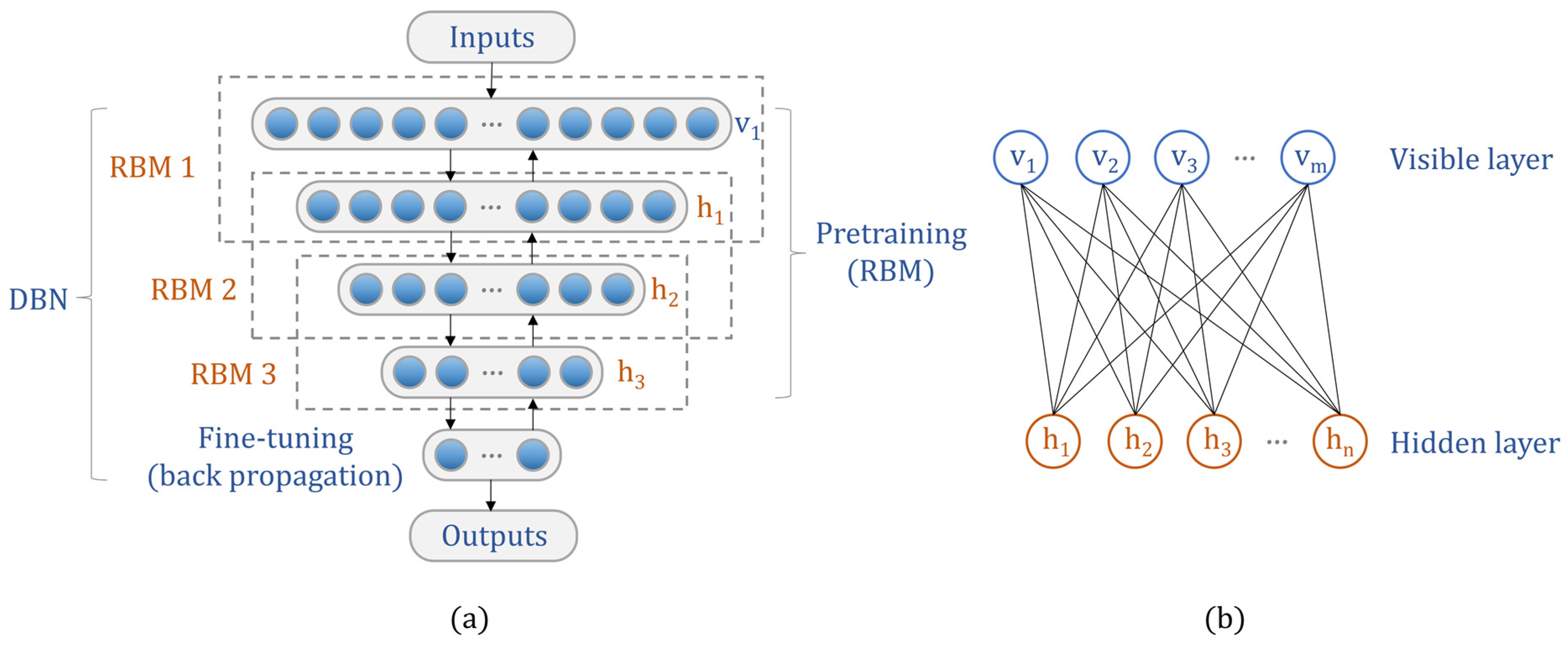
2.1. DBN
2.2. SVR
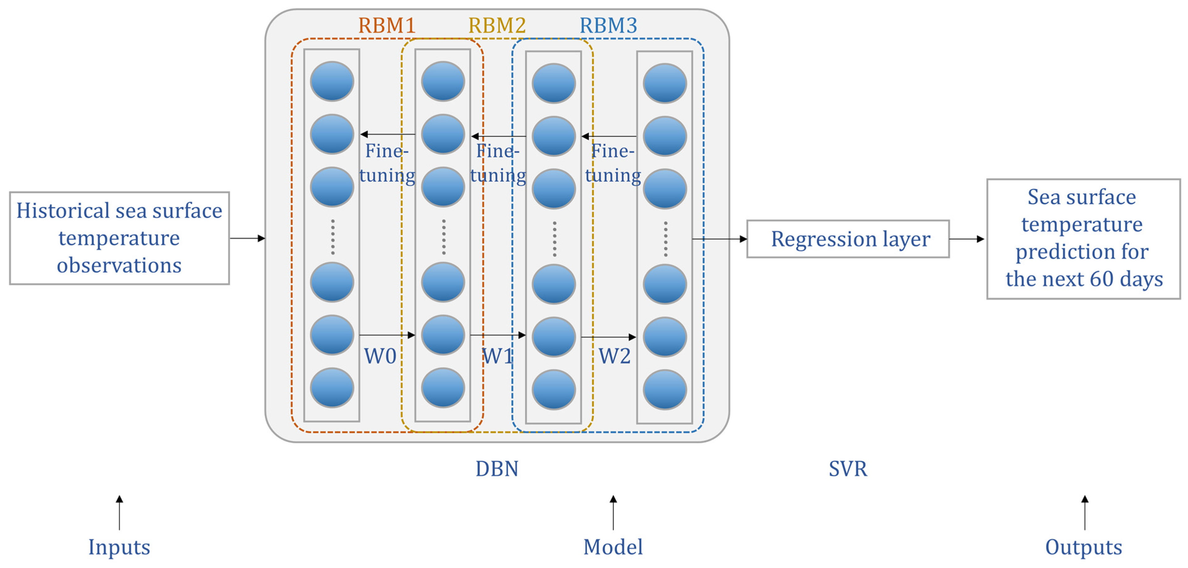
2.3. DBN-SVR
2.4. SSC
| Algorithm 1 Spatiotemporal secondary calibration algorithm |
| Input: |
| Output: |
2.5. Data
2.6. Experimental Design
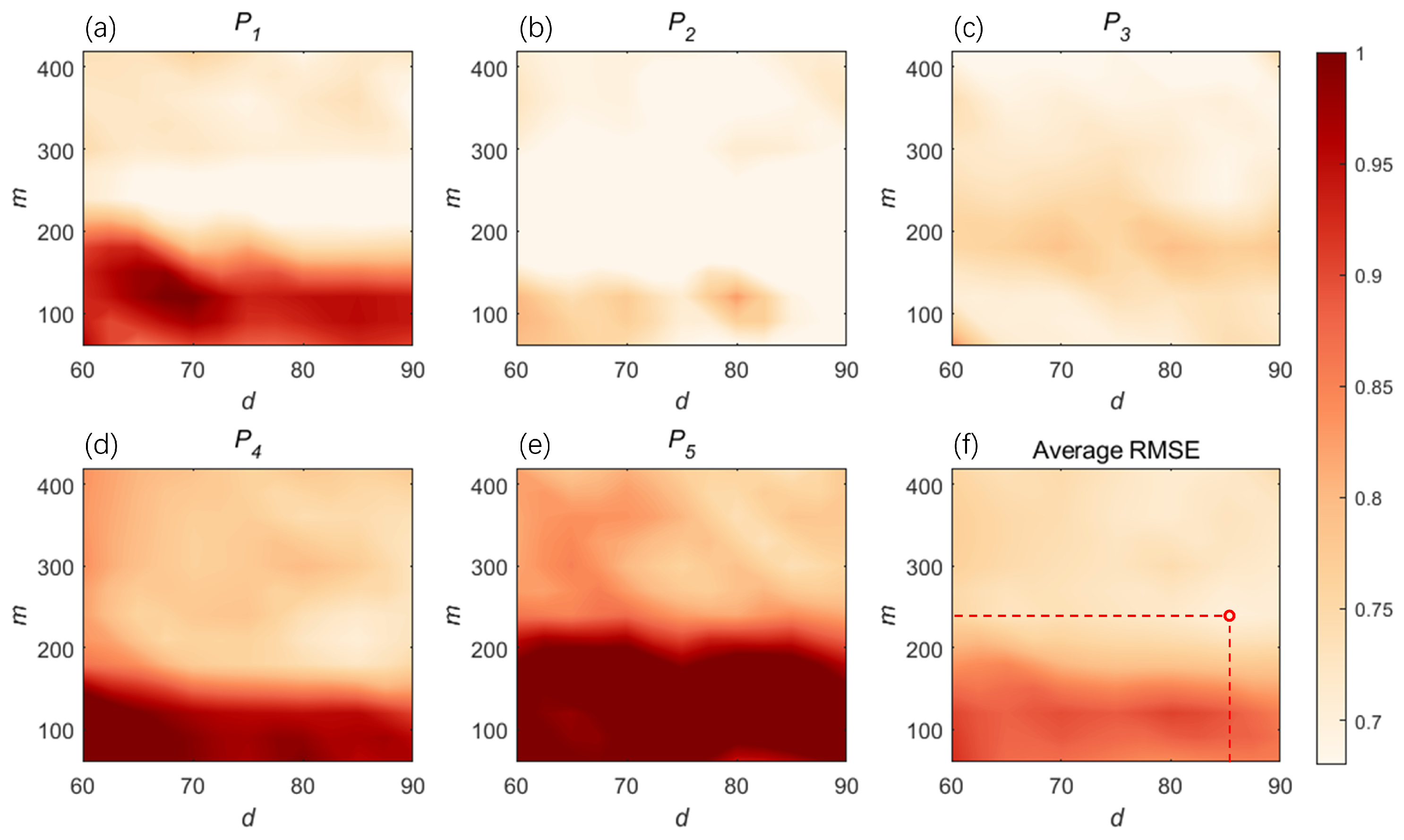
2.7. Parameter Determination
3. Results
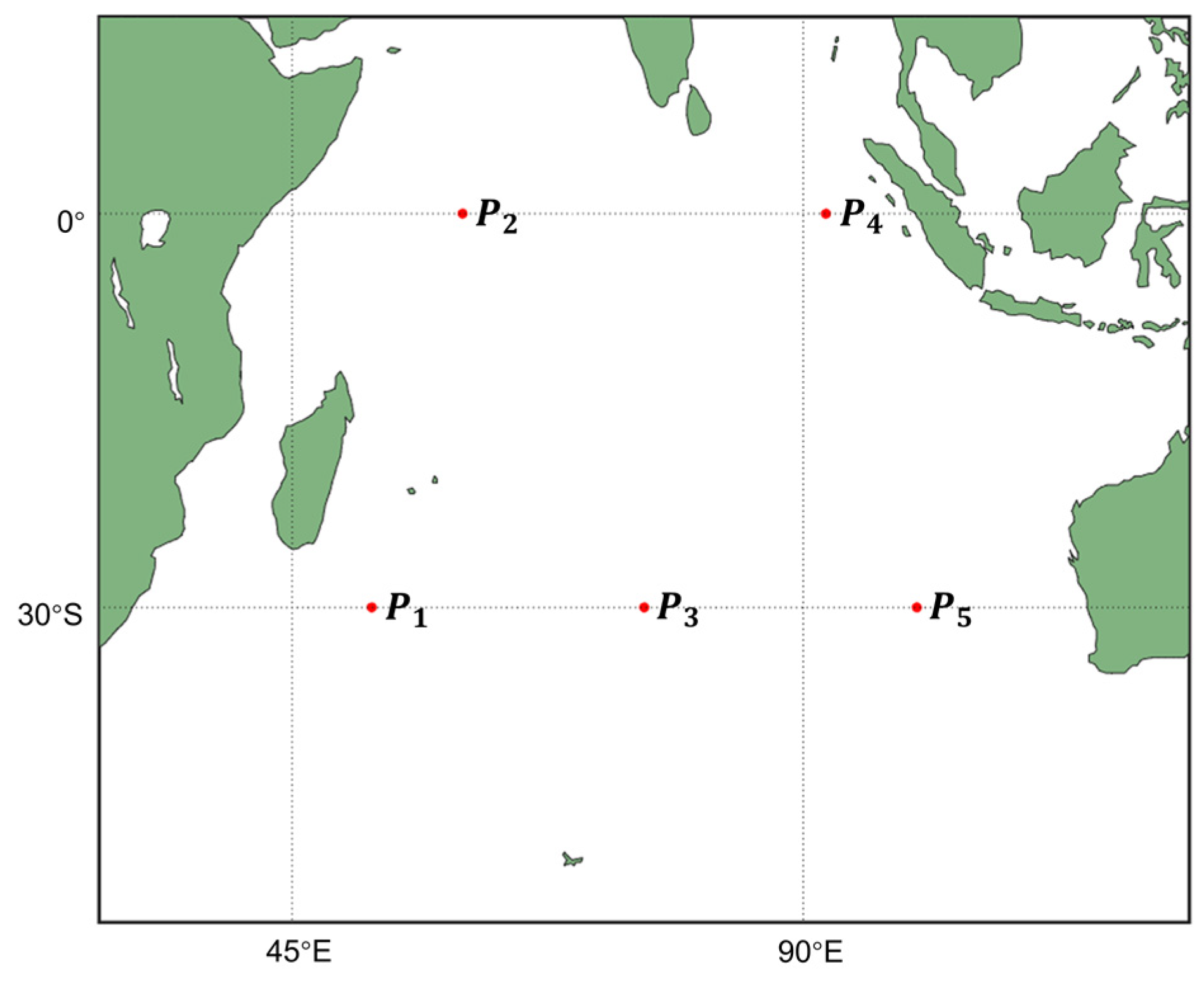
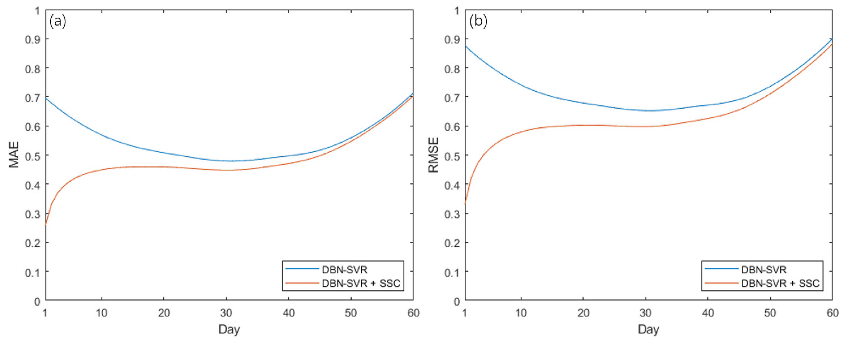
3.1. Results of SSC
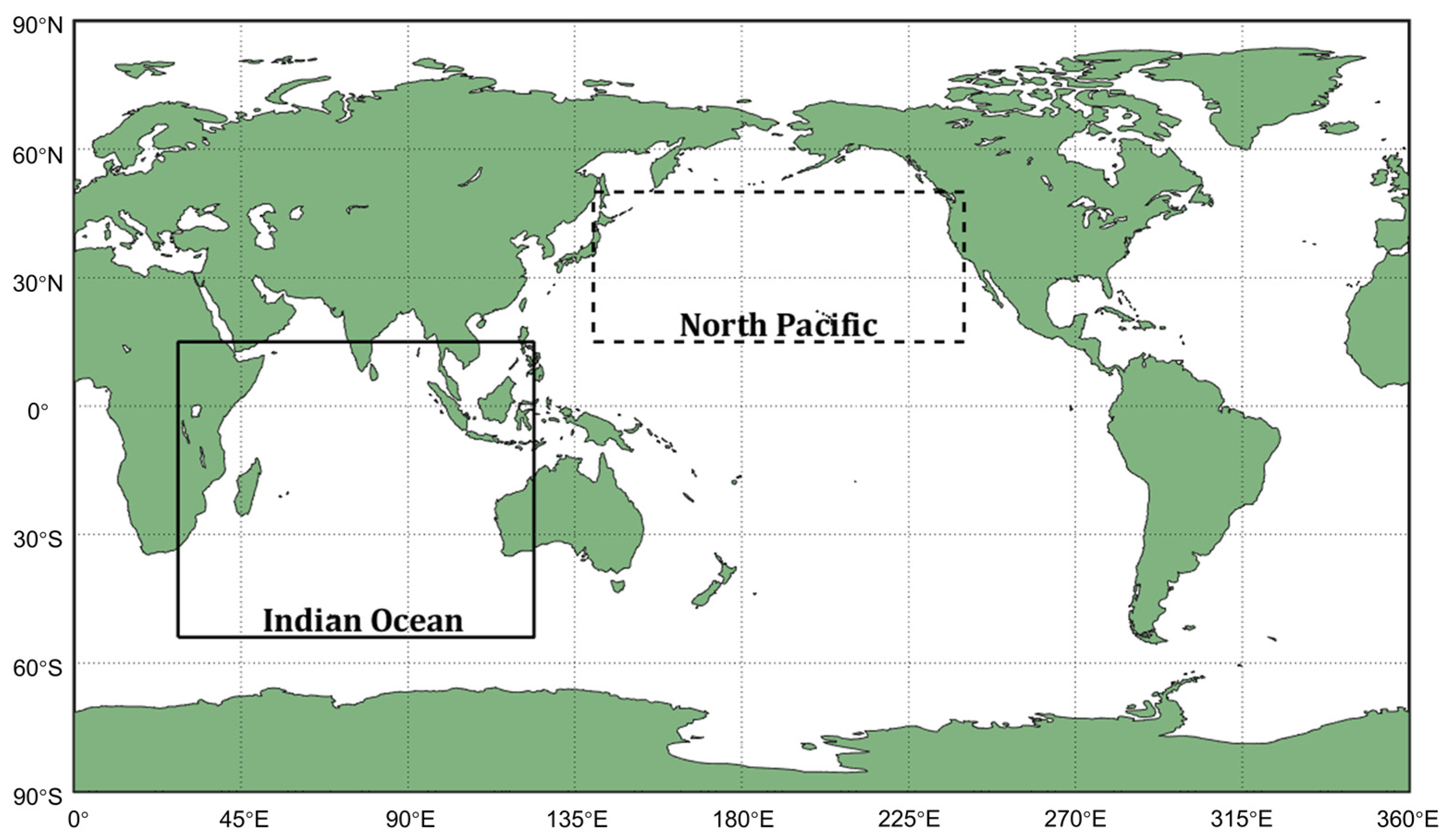
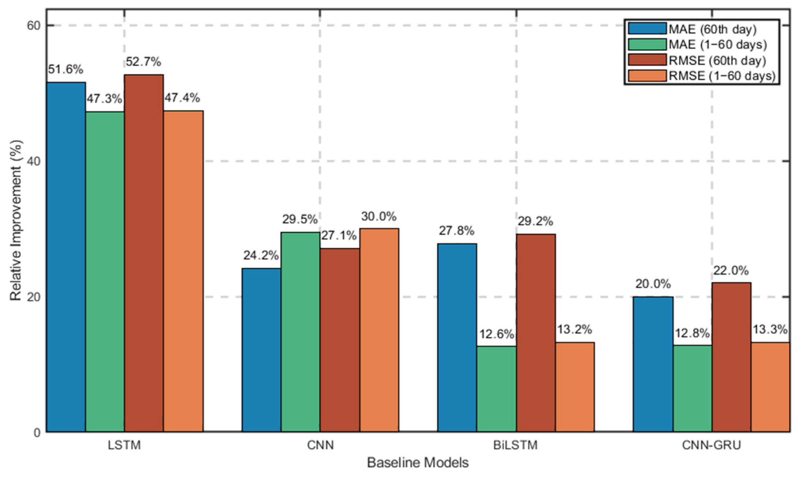
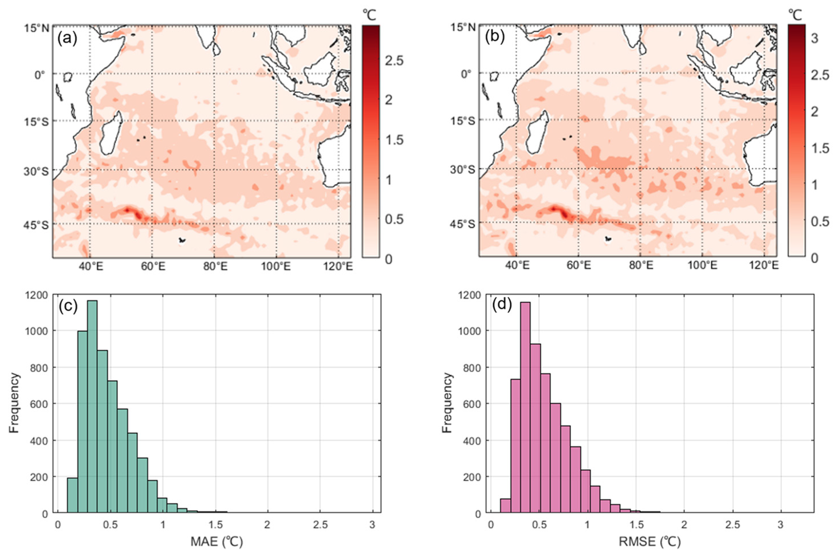
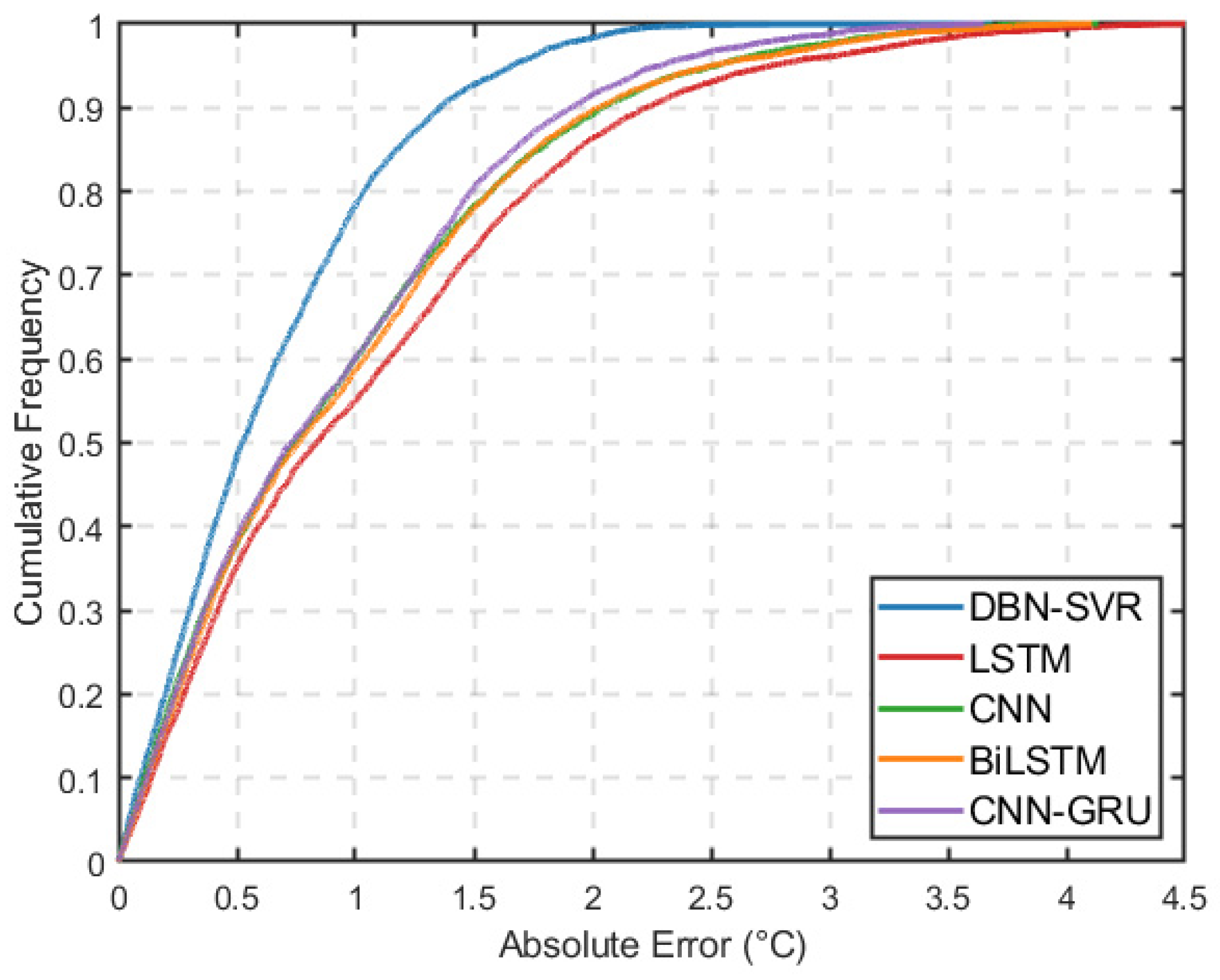
3.2. Results in the Indian Ocean Region
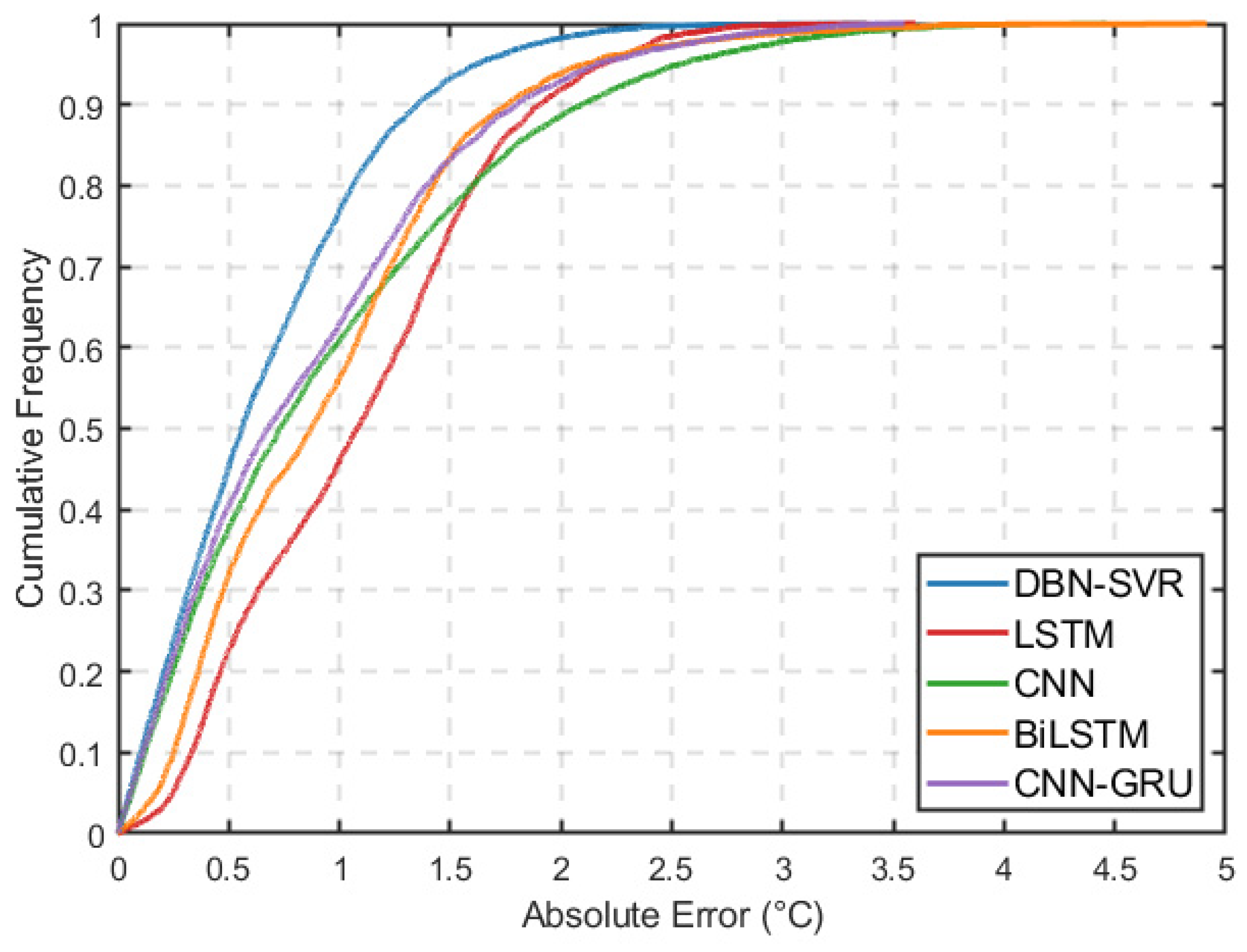
3.3. Results in the North Pacific Region
4. Discussion
5. Conclusions
Author Contributions
Funding
Data Availability Statement
Acknowledgments
Conflicts of Interest
Abbreviations
| SST | Sea surface temperature |
| DBN | Deep belief network |
| SVR | Support vector regression |
| SSC | Spatiotemporal secondary calibration |
| RMSE | Root mean square error |
| MAE | Mean absolute error |
| BP | Back propagation |
| LSTM | Long short-term memory |
| CNN | Convolutional neural networks |
| BiLSTM | Bidirectional long short-term memory |
| TransDtSt-Part | Transformer with temporal embedding, attention distilling, and stacked connection in part |
| RBM | Restricted Boltzmann machine |
| CD | Contrastive divergence |
| RBF | Radial basis function |
| OISSTv2.1 | Optimum Interpolation Sea Surface Temperature version 2.1 |
| AVHRR | Advanced Very High-Resolution Radiometer |
| NOAA | National Oceanic and Atmospheric Administration |
| CNN-GRU | Convolutional neural networks and gated recurrent unit |
| SSA | Sparrow search algorithm |
| CDF | Cumulative distribution function |
Appendix A

| Regions | Metrics | Prediction Duration | |
|---|---|---|---|
| The 60th Day | 1–60 Days Average | ||
| Indian Ocean | MAE (°C) | 0.704 | 0.483 |
| RMSE (°C) | 0.883 | 0.629 | |
| North Pacific Ocean | MAE (°C) | 0.650 | 0.445 |
| RMSE (°C) | 0.853 | 0.608 | |
| South Pacific Ocean | MAE (°C) | 0.772 | 0.460 |
| RMSE (°C) | 0.945 | 0.576 | |
| North Atlantic Ocean | MAE (°C) | 0.870 | 0.571 |
| RMSE (°C) | 1.056 | 0.756 | |
| South Atlantic Ocean | MAE (°C) | 0.812 | 0.443 |
| RMSE (°C) | 0.959 | 0.564 | |
| Arctic Ocean | MAE (°C) | 0.404 | 0.284 |
| RMSE (°C) | 0.721 | 0.513 | |
| Southern Ocean | MAE (°C) | 0.393 | 0.260 |
| RMSE (°C) | 0.628 | 0.387 | |
References
- Bronselaer, B.; Zanna, L. Heat and Carbon Coupling Reveals Ocean Warming Due to Circulation Changes. Nature 2020, 584, 227–233. [Google Scholar] [CrossRef]
- Levitus, S.; Antonov, J.; Boyer, T. Warming of the World Ocean, 1955–2003. Geophys. Res. Lett. 2005, 32, 2004GL021592. [Google Scholar] [CrossRef]
- Chen, Z.; Wen, Z.; Wu, R.; Lin, X.; Wang, J. Relative Importance of Tropical SST Anomalies in Maintaining the Western North Pacific Anomalous Anticyclone during El Niño to La Niña Transition Years. Clim. Dyn. 2016, 46, 1027–1041. [Google Scholar] [CrossRef]
- Kerry, A.E. The Dependence of Hurricane Intensity on Climate. Nature 1987, 326, 483–485. [Google Scholar] [CrossRef]
- Emanuel, K.; Sobel, A. Response of Tropical Sea Surface Temperature, Precipitation, and Tropical Cyclone-Related Variables to Changes in Global and Local Forcing. J. Adv. Model. Earth Syst. 2013, 5, 447–458. [Google Scholar] [CrossRef]
- Vecchi, G.A.; Soden, B.J. Effect of Remote Sea Surface Temperature Change on Tropical Cyclone Potential Intensity. Nature 2007, 450, 1066–1070. [Google Scholar] [CrossRef]
- Holbrook, N.J.; Scannell, H.A.; Sen Gupta, A.; Benthuysen, J.A.; Feng, M.; Oliver, E.C.J.; Alexander, L.V.; Burrows, M.T.; Donat, M.G.; Hobday, A.J.; et al. A Global Assessment of Marine Heatwaves and Their Drivers. Nat. Commun. 2019, 10, 2624. [Google Scholar] [CrossRef]
- TAN, H.-J.; CAI, R.-S.; BAI, D.-P. Causes of 2022 Summer Marine Heatwave in the East China Seas. Adv. Clim. Change Res. 2023, 14, 633–641. [Google Scholar] [CrossRef]
- Xu, T.; Zhou, Z.; Li, Y.; Wang, C.; Liu, Y.; Rong, T. Short-Term Prediction of Global Sea Surface Temperature Using Deep Learning Networks. J. Mar. Sci. Eng. 2023, 11, 1352. [Google Scholar] [CrossRef]
- Hosoda, K. Empirical Method of Diurnal Correction for Estimating Sea Surface Temperature at Dawn and Noon. J. Oceanogr. 2013, 69, 631–646. [Google Scholar] [CrossRef]
- Goela, P.C.; Cordeiro, C.; Danchenko, S.; Icely, J.; Cristina, S.; Newton, A. Time Series Analysis of Data for Sea Surface Temperature and Upwelling Components from the Southwest Coast of Portugal. J. Mar. Syst. 2016, 163, 12–22. [Google Scholar] [CrossRef]
- Majumder, S.; Kanjilal, P.P. Application of Singular Spectrum Analysis for Investigating Chaos in Sea Surface Temperature. Pure Appl. Geophys. 2019, 176, 3769–3786. [Google Scholar] [CrossRef]
- Wei, J.; Liu, X.; Jiang, G. Parameterizing Sea Surface Temperature Cooling Induced by Tropical Cyclones Using a Multivariate Linear Regression Model. Acta Oceanol. Sin. 2018, 37, 1–10. [Google Scholar] [CrossRef]
- Chen, P.; Sun, B. Improving the Dynamical Seasonal Prediction of Western Pacific Warm Pool Sea Surface Temperatures Using a Physical–Empirical Model. Int. J. Climatol. 2020, 40, 4657–4675. [Google Scholar] [CrossRef]
- Zhang, M.; Han, G.; Wu, X.; Li, C.; Shao, Q.; Li, W.; Cao, L.; Wang, X.; Dong, W.; Ji, Z. SST Forecast Skills Based on Hybrid Deep Learning Models: With Applications to the South China Sea. Remote Sens. 2024, 16, 1034. [Google Scholar] [CrossRef]
- Kuang, X.; Wang, Z.; Zhang, M.; He, E.; Deng, X. An interpretation scheme of numerical near-shore sea-water temperature forecast based on bpnn. Oceanol. Limnol. Sin. 2016, 47, 1107–1115. [Google Scholar] [CrossRef]
- Zhang, Q.; Wang, H.; Dong, J.; Zhong, G.; Sun, X. Prediction of Sea Surface Temperature Using Long Short-Term Memory. IEEE Geosci. Remote Sens. Lett. 2017, 14, 1745–1749. [Google Scholar] [CrossRef]
- Yang, Y.; Dong, J.; Sun, X.; Lima, E.; Mu, Q.; Wang, X. A CFCC-LSTM Model for Sea Surface Temperature Prediction. IEEE Geosci. Remote Sens. Lett. 2018, 15, 207–211. [Google Scholar] [CrossRef]
- Zhang, K.; Geng, X.; Yan, X.-H. Prediction of 3-D Ocean Temperature by Multilayer Convolutional LSTM. IEEE Geosci. Remote Sens. Lett. 2020, 17, 1303–1307. [Google Scholar] [CrossRef]
- Weng, S.; Cai, J.; Peng, Y.; Luo, R. Application of convolutional neural networks in nearshore surface sea temperature forecasting. J. Trop. Oceanogr. 2024, 43, 40–47. [Google Scholar] [CrossRef]
- Zrira, N.; Kamal-Idrissi, A.; Farssi, R.; Khan, H.A. Time Series Prediction of Sea Surface Temperature Based on BiLSTM Model with Attention Mechanism. J. Sea Res. 2024, 198, 102472. [Google Scholar] [CrossRef]
- Dai, H.; He, Z.; Wei, G.; Lei, F.; Zhang, X.; Zhang, W.; Shang, S. Long-Term Prediction of Sea Surface Temperature by Temporal Embedding Transformer With Attention Distilling and Partial Stacked Connection. IEEE J. Sel. Top. Appl. Earth Obs. Remote Sens. 2024, 17, 4280–4293. [Google Scholar] [CrossRef]
- Fu, Y.; Song, J.; Guo, J.; Fu, Y.; Cai, Y. Prediction and Analysis of Sea Surface Temperature Based on LSTM-Transformer Model. Reg. Stud. Mar. Sci. 2024, 78, 103726. [Google Scholar] [CrossRef]
- Zhang, G.; Kang, X.; Luo, Y.; Wang, Q.; Song, H.; Yin, X. A Transformer-Based Method for Correcting Daily SST Numerical Forecasting Products. Front. Earth Sci. 2025, 13, 1530475. [Google Scholar] [CrossRef]
- Shi, B.; Ge, C.; Lin, H.; Xu, Y.; Tan, Q.; Peng, Y.; He, H. Sea Surface Temperature Prediction Using ConvLSTM-Based Model with Deformable Attention. Remote Sens. 2024, 16, 4126. [Google Scholar] [CrossRef]
- Ren, J.; Wang, C.; Sun, L.; Huang, B.; Zhang, D.; Mu, J.; Wu, J. Prediction of Sea Surface Temperature Using U-Net Based Model. Remote Sens. 2024, 16, 1205. [Google Scholar] [CrossRef]
- Naskath, J.; Sivakamasundari, G.; Begum, A.A.S. A Study on Different Deep Learning Algorithms Used in Deep Neural Nets: MLP SOM and DBN. Wirel. Pers. Commun. 2023, 128, 2913–2936. [Google Scholar] [CrossRef] [PubMed]
- Balabin, R.M.; Lomakina, E.I. Support Vector Machine Regression (SVR/LS-SVM)—An Alternative to Neural Networks (ANN) for Analytical Chemistry? Comparison of Nonlinear Methods on near Infrared (NIR) Spectroscopy Data. The Analyst 2011, 136, 1703. [Google Scholar] [CrossRef]
- Liu, Y.; Fan, Y.; Chen, J. Flame Images for Oxygen Content Prediction of Combustion Systems Using DBN. Energy Fuels 2017, 31, 8776–8783. [Google Scholar] [CrossRef]
- Li, Z.; Ge, X. Prediction And Analysis Of Road Traffic Efficiency Based on DBN-SVR. In Proceedings of the 2019 1st International Conference on Industrial Artificial Intelligence (IAI), Shenyang, China, 23–27 July 2019; pp. 1–6. [Google Scholar]
- Smith, T.; Reynolds, R.; Peterson, T.; Lawrimore, J. Improvements to NOAA’s Historical Merged Land–Ocean Surface Temperature Analysis (1880–2006). J. Clim. 2008, 21, 2283–2296. [Google Scholar] [CrossRef]
- Yan, J.; Gao, Y.; Yu, Y.; Xu, H.; Xu, Z. A Prediction Model Based on Deep Belief Network and Least Squares SVR Applied to Cross-Section Water Quality. Water 2020, 12, 1929. [Google Scholar] [CrossRef]
- Hinton, G.E.; Osindero, S.; Teh, Y.-W. A Fast Learning Algorithm for Deep Belief Nets. Neural Comput. 2006, 18, 1527–1554. [Google Scholar] [CrossRef] [PubMed]
- Tao, H.; Sulaiman, S.O.; Yaseen, Z.M.; Asadi, H.; Meshram, S.G.; Ghorbani, M.A. What Is the Potential of Integrating Phase Space Reconstruction with SVM-FFA Data-Intelligence Model? Application of Rainfall Forecasting over Regional Scale. Water Resour. Manag. 2018, 32, 3935–3959. [Google Scholar] [CrossRef]
- Sun, Y.; Ding, S.; Zhang, Z.; Jia, W. An Improved Grid Search Algorithm to Optimize SVR for Prediction. Soft Comput. 2021, 25, 5633–5644. [Google Scholar] [CrossRef]
- Wang, G.; Fan, H. Prediction Model of Blood Pressure during Hemodialysis Base on Deep Learning. In Proceedings of the 2021 7th International Conference on Computing and Artificial Intelligence, Tianjin, China, 23–26 April 2021; pp. 431–436. [Google Scholar] [CrossRef]
- Le Grix, N.; Zscheischler, J.; Rodgers, K.B.; Yamaguchi, R.; Frölicher, T.L. Hotspots and Drivers of Compound Marine Heatwaves and Low Net Primary Production Extremes. Biogeosciences 2022, 19, 5807–5835. [Google Scholar] [CrossRef]
- Lu, Z.; Dong, W.; Lu, B.; Yuan, N.; Ma, Z.; Bogachev, M.I.; Kurths, J. Early Warning of the Indian Ocean Dipole Using Climate Network Analysis. Proc. Natl. Acad. Sci. USA 2022, 119, e2109089119. [Google Scholar] [CrossRef]
- Gunnarson, J.L.; Stuecker, M.F.; Zhao, S. Drivers of Future Extratropical Sea Surface Temperature Variability Changes in the North Pacific. Npj Clim. Atmos. Sci. 2024, 7, 164. [Google Scholar] [CrossRef]
- Pan, X.; Jiang, T.; Sun, W.; Xie, J.; Wu, P.; Zhang, Z.; Cui, T. Effective Attention Model for Global Sea Surface Temperature Prediction. Expert Syst. Appl. 2024, 254, 124411. [Google Scholar] [CrossRef]
- Schott, F.A.; Xie, S.-P.; McCreary, J.P., Jr. Indian Ocean Circulation and Climate Variability. Rev. Geophys. 2009, 47. [Google Scholar] [CrossRef]
- Di Lorenzo, E.; Cobb, K.M.; Furtado, J.C.; Schneider, N.; Anderson, B.T.; Bracco, A.; Alexander, M.A.; Vimont, D.J. Central Pacific El Niño and Decadal Climate Change in the North Pacific Ocean. Nat. Geosci. 2010, 3, 762–765. [Google Scholar] [CrossRef]
- Irrgang, C.; Saynisch-Wagner, J.; Thomas, M. Machine Learning-Based Prediction of Spatiotemporal Uncertainties in Global Wind Velocity Reanalyses. J. Adv. Model. Earth Syst. 2020, 12, e2019MS001876. [Google Scholar] [CrossRef]
- Cheng, Q.; Chen, Y.; Xiao, Y.; Yin, H.; Liu, W. A Dual-Stage Attention-Based Bi-LSTM Network for Multivariate Time Series Prediction. J. Supercomput. 2022, 78, 16214–16235. [Google Scholar] [CrossRef]
- Alizadegan, H.; Rashidi Malki, B.; Radmehr, A.; Karimi, H.; Ilani, M.A. Comparative Study of Long Short-Term Memory (LSTM), Bidirectional LSTM, and Traditional Machine Learning Approaches for Energy Consumption Prediction. Energy Explor. Exploit. 2024, 10, 3315–3334. [Google Scholar] [CrossRef]
- Wang, J.; Wang, P.; Tian, H.; Tansey, K.; Liu, J.; Quan, W. A Deep Learning Framework Combining CNN and GRU for Improving Wheat Yield Estimates Using Time Series Remotely Sensed Multi-Variables. Comput. Electron. Agric. 2023, 206, 107705. [Google Scholar] [CrossRef]
- Chen, Y.; Xu, P.; Chu, Y.; Li, W.; Wu, Y.; Ni, L.; Bao, Y.; Wang, K. Short-Term Electrical Load Forecasting Using the Support Vector Regression (SVR) Model to Calculate the Demand Response Baseline for Office Buildings. Appl. Energy 2017, 195, 659–670. [Google Scholar] [CrossRef]


| Models | Metrics | Prediction Duration | |||
|---|---|---|---|---|---|
| The 60th Day | 1–60 Days Average | 1–30 Days Average | 31–60 Days Average | ||
| DBN-SVR | MAE (°C) | 0.714 | 0.549 | 0.549 | 0.549 |
| RMSE (°C) | 0.902 | 0.724 | 0.721 | 0.726 | |
| DBN-SVR + SSC | MAE (°C) | 0.704 | 0.483 | 0.435 | 0.530 |
| RMSE (°C) | 0.883 | 0.629 | 0.567 | 0.691 | |
| Models | Metrics | Prediction Duration | |
|---|---|---|---|
| The 60th Day | 1–60 Days Average | ||
| DBN-SVR | MAE (°C) | 0.704 | 0.483 |
| RMSE (°C) | 0.883 | 0.629 | |
| LSTM | MAE (°C) | 1.456 | 0.915 |
| RMSE (°C) | 1.868 | 1.197 | |
| CNN | MAE (°C) | 0.929 | 0.689 |
| RMSE (°C) | 1.212 | 0.899 | |
| BiLSTM | MAE (°C) | 0.975 | 0.552 |
| RMSE (°C) | 1.247 | 0.725 | |
| CNN-GRU | MAE (°C) | 0.880 | 0.553 |
| RMSE (°C) | 1.132 | 0.726 | |
| Models | Metrics | Prediction Duration | |
|---|---|---|---|
| The 60th Day | 1–60 Days Average | ||
| DBN-SVR | MAE (°C) | 0.650 | 0.445 |
| RMSE (°C) | 0.853 | 0.608 | |
| LSTM | MAE (°C) | 1.306 | 0.930 |
| RMSE (°C) | 1.642 | 1.196 | |
| CNN | MAE (°C) | 0.934 | 0.627 |
| RMSE (°C) | 1.217 | 0.825 | |
| BiLSTM | MAE (°C) | 1.093 | 0.698 |
| RMSE (°C) | 1.267 | 0.917 | |
| CNN-GRU | MAE (°C) | 0.843 | 0.508 |
| RMSE (°C) | 1.085 | 0.662 | |
Disclaimer/Publisher’s Note: The statements, opinions and data contained in all publications are solely those of the individual author(s) and contributor(s) and not of MDPI and/or the editor(s). MDPI and/or the editor(s) disclaim responsibility for any injury to people or property resulting from any ideas, methods, instructions or products referred to in the content. |
© 2025 by the authors. Licensee MDPI, Basel, Switzerland. This article is an open access article distributed under the terms and conditions of the Creative Commons Attribution (CC BY) license (https://creativecommons.org/licenses/by/4.0/).
Share and Cite
Liu, Y.; Zhao, Z.; Zhang, Z.; Yang, Y. A Novel Sea Surface Temperature Prediction Model Using DBN-SVR and Spatiotemporal Secondary Calibration. Remote Sens. 2025, 17, 1681. https://doi.org/10.3390/rs17101681
Liu Y, Zhao Z, Zhang Z, Yang Y. A Novel Sea Surface Temperature Prediction Model Using DBN-SVR and Spatiotemporal Secondary Calibration. Remote Sensing. 2025; 17(10):1681. https://doi.org/10.3390/rs17101681
Chicago/Turabian StyleLiu, Yibo, Zichen Zhao, Zhe Zhang, and Yi Yang. 2025. "A Novel Sea Surface Temperature Prediction Model Using DBN-SVR and Spatiotemporal Secondary Calibration" Remote Sensing 17, no. 10: 1681. https://doi.org/10.3390/rs17101681
APA StyleLiu, Y., Zhao, Z., Zhang, Z., & Yang, Y. (2025). A Novel Sea Surface Temperature Prediction Model Using DBN-SVR and Spatiotemporal Secondary Calibration. Remote Sensing, 17(10), 1681. https://doi.org/10.3390/rs17101681