Article

Evaluating Arctic Thin Ice Thickness Retrieved from Latest Version of Multisource Satellite Products

1
College of Oceanography and Ecological Science, Shanghai Ocean University, Shanghai 201306, China
2
College of Meteorology and Oceanography, National University of Defense Technology, Changsha 410073, China
3
School for Marine Science and Technology, University of Massachusetts-Dartmouth, New Bedford, MA 02744, USA
4
School of Oceanography, Shanghai Jiao Tong University, Shanghai 200030, China
5
First Institute of Oceanography and Key Laboratory of Marine Science and Numerical Modeling, Ministry of Natural Resources, Qingdao 266061, China
*
Author to whom correspondence should be addressed.
These authors contributed equally to this work.
Remote Sens. 2025, 17(10), 1680; https://doi.org/10.3390/rs17101680 (registering DOI)
Submission received: 2 March 2025 / Revised: 30 April 2025 / Accepted: 8 May 2025 / Published: 10 May 2025

Abstract

:
Currently, the performance of sea ice thickness (SIT) data retrieved from multisource satellite products in the Arctic seasonal ice zones remains unclear. This study presented the spatiotemporal intercomparison and evaluation of satellite data, including the latest versions of Soil Moisture and Ocean Salinity (SMOS), CryoSat-2, combined CryoSat-2 and SMOS (CS2SMOS), and Ice, Cloud, and Land Elevation Satellite-2 (ICESat-2), specifically focusing on area with mean SIT below 0.5 m. Five evaluation datasets were used. During 2010–2023, SMOS had the smallest mean SIT, with CryoSat-2 showing the largest mean SIT. During 2018–2023, with the inclusion of ICESat-2, SMOS still showed the smallest mean SIT. CryoSat-2 exhibited the largest mean SIT, followed by ICESat-2, CS2SMOS ranked third. Evaluation results indicated that four satellite products generally underestimated SIT. In two periods, SMOS consistently exhibited the weakest performance, which showed a large gap from what was expected in previous studies. In contrast, CS2SMOS demonstrated the highest alignment with five evaluation datasets during 2010–2023, indicating the best overall performance. During 2018–2023, ICESat-2 exhibited the best overall performance with two evaluation datasets. This study refreshes previous knowledge about SMOS in the seasonal ice zones and contributes to further improvements in SIT retrieval.

1. Introduction

Sea ice, as a critical component of the Arctic marine system, plays a vital role in regulating the global climate system. Its high albedo contributes to the Earth’s energy balance by reflecting solar radiation and thereby limiting the amount of heat entering the Arctic Ocean [1]. Additionally, sea ice modulates the exchange of heat, moisture, and momentum between the ocean and the atmosphere, thereby influencing global climate patterns and ocean circulation [2,3]. In the past decades, Arctic sea ice thickness (SIT) has experienced significant reductions. The sea ice draft data collected by US Navy submarines decreased by 1.13 m from 1980 to 2000, equivalent to a reduction of 1.25 m in SIT [4]. In the Central Arctic Basin area, the average SIT declined from 3.59 m in 1975 to 1.25 m in 2012, indicating a 65% reduction [5]. Over the six decades between 1958 and 2018, the average SIT in most areas of the Arctic decreased by approximately 2 m at the end of the melting season [6]. From 2018 to 2021, the multi-year ice in the Arctic region thinned by approximately 0.50 m, and the average thickness of Arctic sea ice in spring decreased by about 0.28 m [7]. The reduction in Arctic sea ice has also created more opportunities for navigation in the Arctic region [8,9].
Relative to Arctic sea ice concentration, the collection of SIT data is limited. Presently, SIT observation data can be collected by various methods. For example, drilling holes to measure SIT is a direct observational method that entails drilling into the surface of the sea ice, penetrating down to the water column beneath, and then gauging the depth of the hole [10]. The U.S. Navy installed upward-looking sonars (ULSs) on naval submarines and on moorings to observe sea ice draft [11]. Richter-Menge et al. [12] developed an autonomous ice mass-balance buoy (IMB), which is equipped with sensors to measure snow accumulation and ablation and ice growth and melt. NASA Operation IceBridge mission utilized a suite of instruments, including radar and laser altimeters, to measure sea ice freeboard and snow depth data [13]. The hydrostatic balance equation was then used to calculate SIT by combining the sea ice freeboard and snow depth data. Using helicopter electromagnetics, it was possible to estimate the thickness of sea ice based on the principle of electromagnetic induction, by measuring changes in the secondary magnetic field generated by a transmitting coil [14]. However, the SIT observation data obtained by these measurement methods are limited in terms of spatiotemporal coverage. The satellite provides an opportunity to cover a large-scale area and offer high spatial resolution for observation. In recent decades, various satellites have been applied to SIT observations. The Ice, Cloud, and Land Elevation Satellite (ICESat) and its successor, the Ice, Cloud, and Land Elevation Satellite-2 (ICESat-2), both utilize laser altimeters to measure SIT [15,16]. ICESat operated from 2003 to 2008, while ICESat-2 commenced its measurements in 2018. The CryoSat-2 product, boasting a synthetic aperture radar/Interferometric Radar Altimeter, commenced its operations in 2010 [17]. The Soil Moisture and Ocean Salinity (SMOS) satellite, equipped with the Microwave Imaging Radiometer with Aperture Synthesis (MIRAS) operating at 1.4 GHz in the L-band, started its operations in 2010 [18]. The CS2SMOS product combined data from CryoSat-2 and SMOS and was developed through a collaboration between the Alfred Wegener Institute (AWI) and the University of Hamburg [19].
Due to differences in measurement techniques and data processing methods, satellite products exhibit significant discrepancies in SIT measurements. Some studies have been conducted to evaluate satellite SIT products in the Arctic region [20,21,22,23,24]. However, due to higher measurement errors in thicker ice regions, SMOS data are usually excluded from these analyses. Additionally, previous studies have focused on SIT assessments across the entire Arctic; there are relatively few studies specifically targeting seasonal ice zones (<0.5 m). SMOS data are generally considered more reliable for seasonal ice zones (<0.5 m). Tian-Kunze et al. [25] mentioned that the uncertainty of SIT obtained by SMOS is lower in the thin ice range (<0.5 m) compared to measurements from ICESat and CryoSat-2. Tietsche et al. [26] mentioned that laser and radar altimetry are not practical for measuring SIT below 0.5 m. However, the quantitative evaluation of SMOS performance for SIT retrieval below 0.5 m has not been conducted in previous studies.
Therefore, we aim to further extend and complement previous work by evaluating the performance of SMOS in zones with SIT below 0.5 m in this study. To clarify the retrieval accuracy of SMOS data in seasonal ice zones, we incorporate additional satellite data as references, including CryoSat-2, CS2SMOS, and ICESat-2, for comparative analysis. Notably, between October and December 2023, CS2SMOS, CryoSat-2, and ICESat-2 successively released the latest versions, in which the data processing algorithms were improved [27]. The performance of these updated data in seasonal ice zones compared to SMOS remains unclear. In this study, regions where the mean SIT obtained by SMOS from October to December and January to April between 2010 and 2023 is less than 0.5 m are defined as the seasonal ice zones. Four types of datasets from airborne and in situ measurements were comprehensively utilized as evaluation data. Intercomparing and evaluating multisource satellite SIT data enhances the understanding of the performance of different satellite products in seasonal ice zones.

2. Materials and Methods

2.1. Satellite Product Data

2.1.1. SMOS

Launched in November 2009, the SMOS satellite is dedicated to providing crucial data on land surface soil moisture and ocean surface salinity. In addition to its primary objectives, SMOS also serves as a valuable tool for retrieving sea ice information, including SIT. The SMOS mission provides L-band brightness temperature observations ideal for gauging the thickness of thin sea ice areas [25,28]. The SIT retrieval relies on an empirical relationship between brightness temperature and ice thickness. By modeling the emissivity of sea ice based on its temperature and salinity, and using known brightness temperatures for open water and thick ice as reference points, the ice thickness can be derived from the observed brightness temperatures. The latest version 3.3 daily SMOS SIT data, released by AWI in November 2021, was utilized. SMOS provides a spatial resolution of 12.5 km and covers the sea ice growth period from October to April of the following year. The study period spans from October 2010 to April 2023.

2.1.2. CryoSat-2

The CryoSat-2 satellite, launched by the European Space Agency (ESA) in 2010, aims to measure changes in polar ice sheets and sea ice [29]. The CryoSat-2 product primarily estimates SIT through the analysis of radar waveforms. Specifically, the surface elevation is derived using the Threshold First Maximum Retracker Algorithm (TFMRA) with corrections for atmospheric and oceanographic effects. Leads are detected based on waveform shape parameters, and sea surface elevation is calculated by subtracting a mean sea surface and interpolating sea level anomalies between leads. Snow depth is estimated using a merged climatology of Warren et al. [30] and AMSR2 data. The ice freeboard is then derived by subtracting sea surface height from the measured surface elevation. Finally, SIT is computed by converting the freeboard into thickness while accounting for snow depth under the assumption of hydrostatic equilibrium. CryoSat-2 estimates SIT by measuring the freeboard of the ice and snow cover. The latest version 2.6 monthly CryoSat-2 SIT data, released by AWI in November 2023, was utilized. CryoSat-2 covers the sea ice growth season from October to April, with a spatial resolution of 25 km. The study period spans from October 2010 to April 2023.

2.1.3. CS2SMOS

The CS2SMOS SIT product, a collaborative effort between AWI and the University of Hamburg, combines CS2 and SMOS thickness estimates [19]. CS2 uses radar altimetry to measure sea ice thickness based on hydrostatic equilibrium, effective for thicker multiyear ice. SMOS measures L-band brightness temperatures to estimate thin ice thickness during freeze-up, with an upper limit of around 1.1 m for reliable estimates. The CS2SMOS merging algorithm combines these datasets using Optimal Interpolation (OI), weighting data by uncertainties, and applying a spatial covariance model to minimize errors. The latest version, 2.6, was released in October 2023. The spatial resolution and study period for CS2SMOS align with those of CryoSat-2.

2.1.4. ICESat-2

ICESat-2, launched in 2018, aims to extend the scientific mission of ICESat by offering enhanced precision and spatial resolution in its measurements. Equipped with the Advanced Topographic Laser Altimeter System (ATLAS), ICESat-2 utilizes cutting-edge multi-beam technology to deliver more densely sampled data [31]. ICESat-2 estimates surface elevation by analyzing photon returns from its ATLAS laser altimeter. Leads are detected by identifying regions with distinct photon characteristics, and sea surface elevation is calculated from these lead measurements. Snow depth is estimated using models like NASA Eulerian Snow on Sea Ice Model (NESOSIM v1.0) [32]. The freeboard is then derived by subtracting the sea surface elevation from the measured surface elevation. Finally, SIT is computed by considering the freeboard and snow depth, effectively converting the freeboard into SIT while accounting for the impact of snow cover on the overall ice thickness. The study utilized the latest version of ICESat-2 monthly SIT data, released by the U.S. National Snow and Ice Data Center (NSIDC) in December 2023. ICESat-2 also covers the sea ice growth season from October to April. The study period ranges from November 2018 to April 2023, with a spatial resolution of 25 km.

2.2. Evaluation Data

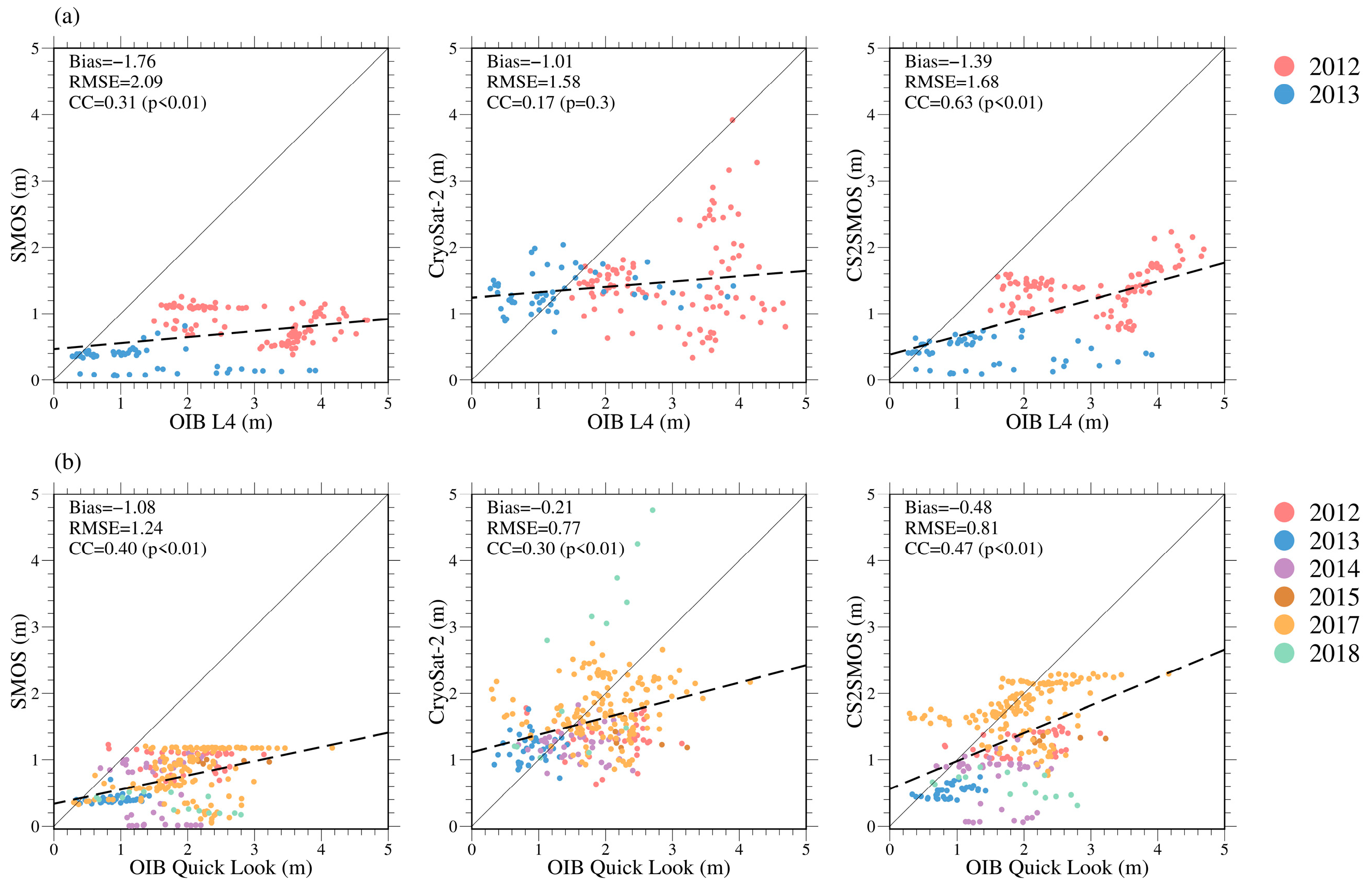
2.2.1. Operation IceBridge (OIB)

The daily OIB dataset was designed to bridge the observational gap between the end of ICESat’s scientific data collection in 2009 and the launch of ICESat-2 in late 2018, ensuring continuous monitoring of polar regions. This study utilized two versions of the data: OIB L4 [33] and OIB Quick Look [34]. The OIB L4 dataset, covering the period from 2012 to 2013, has been validated and shown to be consistent with independent datasets [13]. Although the OIB Quick Look dataset incorporates additional uncertainty, it extends the observational period, covering from 2012 to 2018. The monthly averages of the datasets used in this study represent only the averages of the valid ice record. The tracks of both the OIB L4 and OIB Quick Look datasets can be found in Figure 1.

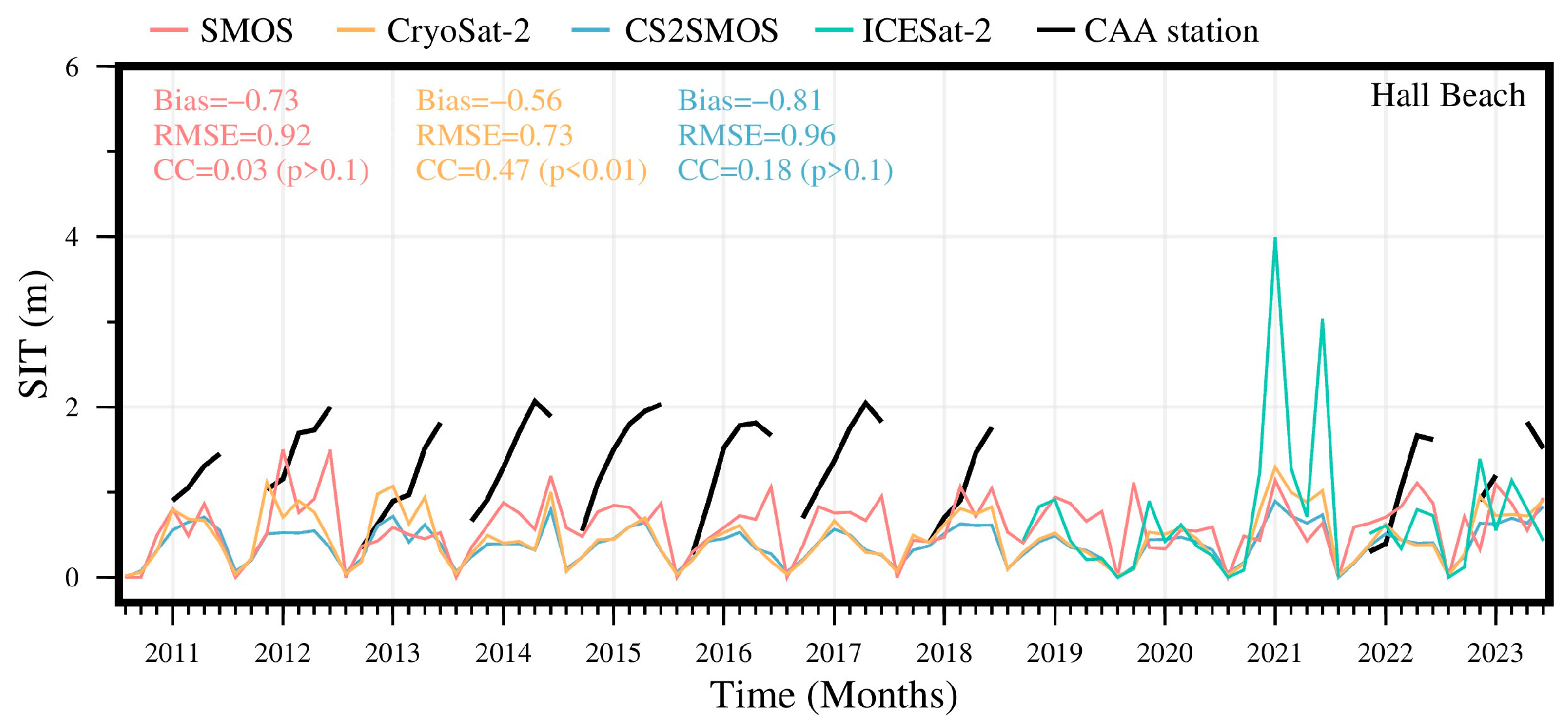
2.2.2. Canadian Arctic Archipelago Station (CAA Station)

The Canadian Ice Service provided daily in situ SIT observation data for the CAA station from 2011 to 2023. Measurements were conducted weekly by drilling holes at nearly identical locations each year. The monthly averages of the data used in this study represent only the averages of the valid ice record. In the seasonal ice zones covered by this study, only one station was available (Figure 1).

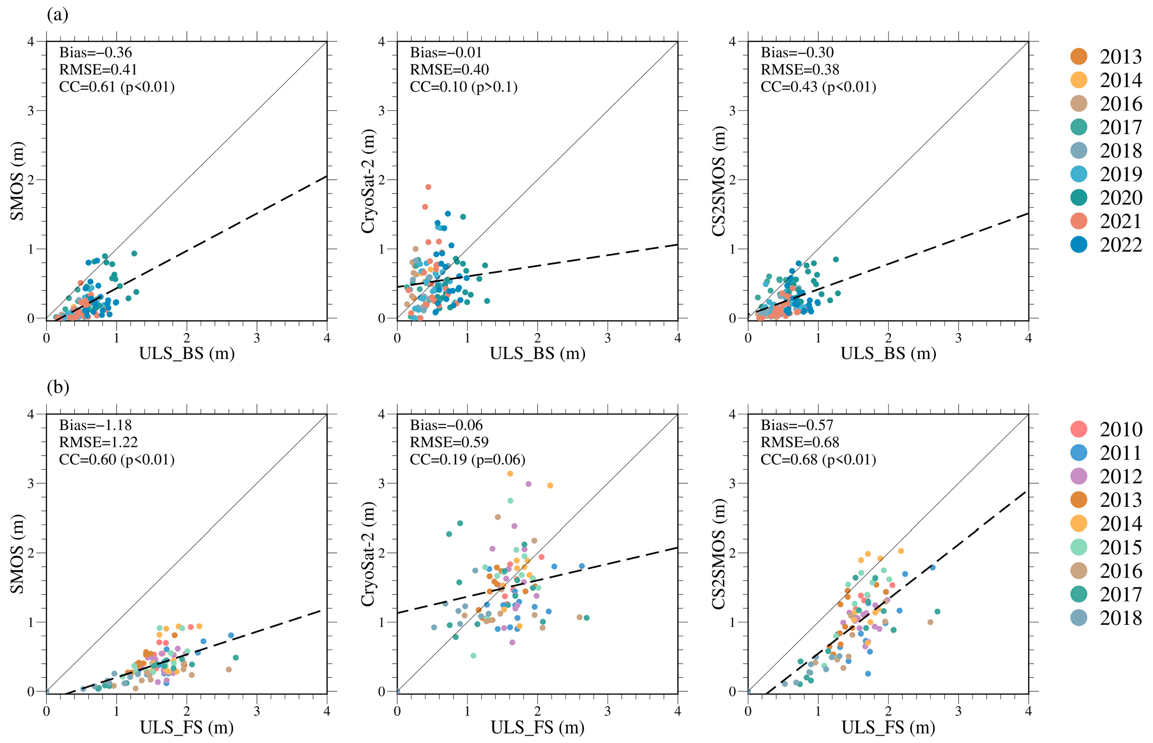
2.2.3. ULS Measurements in the Barents Sea (ULS_BS)

The daily sea ice draft measurements from moored Upward Looking Sonars (ULSs) instruments in the northwestern Barents Sea have been collected regularly since 2013 [35]. The moorings are usually retrieved and redeployed in October. These instruments are Ice Profiling Sonar 5 (IPS5) models from ASL Environmental Sciences, which measure sea ice draft every 1 s with an accuracy of ±0.05 m [36,37]. For this study, the data span from 2013 to 2022. The monthly averages of the data used in this study represent only the averages of the valid ice record. The SIT calculation method follows Fukamachi et al. [38], where the sea ice draft measurements are multiplied by 1.1 to estimate SIT. The mooring locations are shown in Figure 1.

2.2.4. ULS Measurements in Fram Strait (ULS_FS)

The dataset provides monthly mean sea ice draft from the Fram Strait Arctic Outflow Observatory since 1990 [39]. The sea ice draft is measured using ULS and IPS deployed on an east–west oriented mooring array in the western Fram Strait. For this study, the data span from 2010 to 2018. The processing method is consistent with ULS_BS. The mooring locations are shown in Figure 1.

2.3. Intercomparison Methods of Satellite Products

To ensure consistency among various satellite products, the Inverse Distance Weighting (IDW) method was employed to interpolate the area north of 65°N onto a grid with a resolution of 12.5 × 12.5 km. Given that ICESat-2 data start in 2018, this study is divided into two intercomparison periods: the first period, from 2010 to 2023, focuses on intercomparing SMOS, CryoSat-2, and CS2SMOS; the second period, from 2018 to 2023, includes intercomparisons among SMOS, CryoSat-2, CS2SMOS, and ICESat-2.
To meticulously examine the regional variations among these satellite products, the region of thin ice is partitioned into 6 distinct sub-regions: Chukchi Sea, Laptev Sea, Kara Sea, Barents Sea, Greenland Sea, and Baffin Island (as depicted in Figure 1). In the evaluation of consistency and similarity among different satellite products, metrics such as Bias, root mean squared error (RMSE), and correlation coefficient (CC) were utilized.

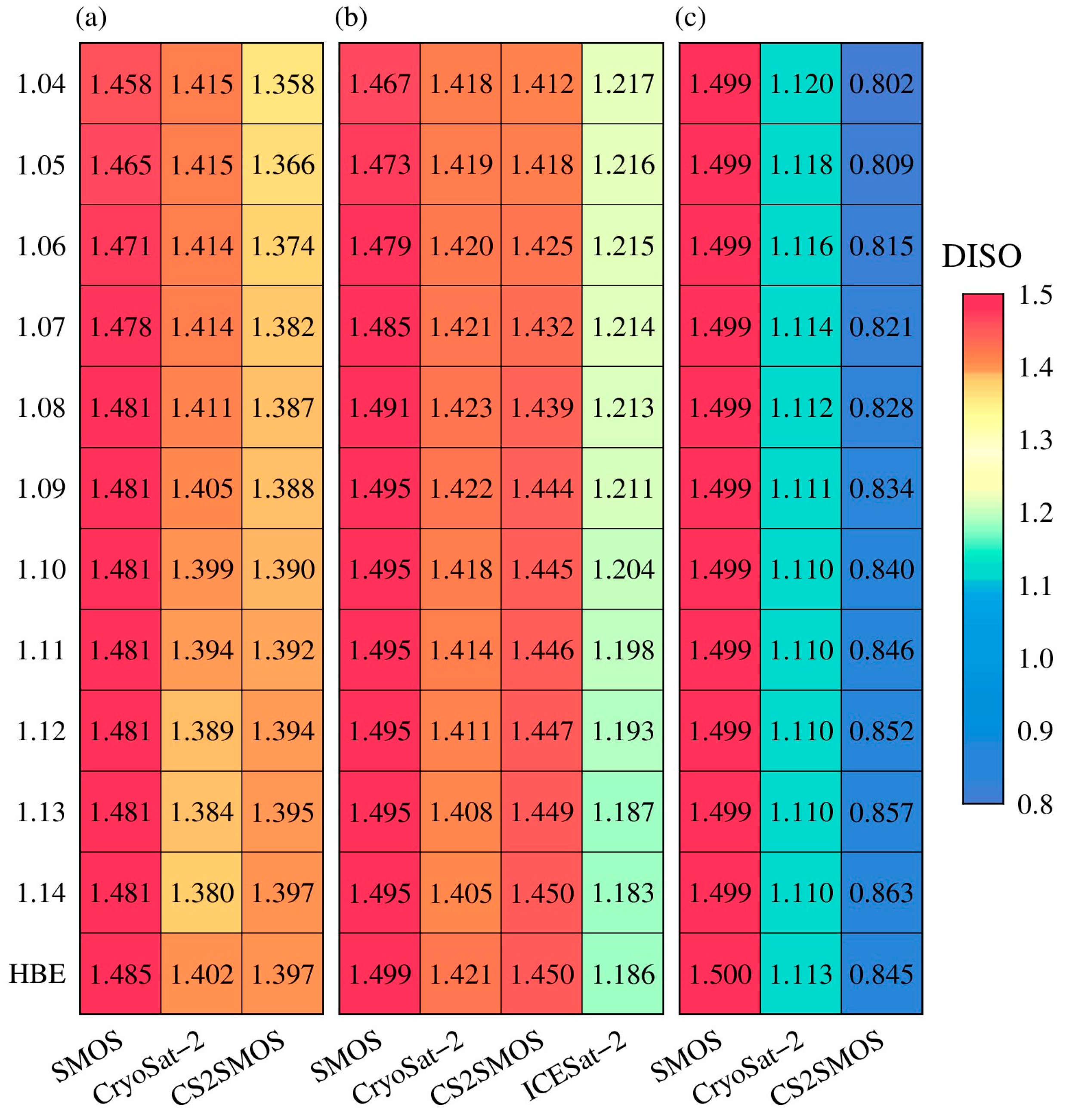
2.4. Evaluation Methods of Satellite Products

The evaluation period for satellite products is divided into two groups: 2010–2023 and 2018–2023. To evaluate multisource satellite SIT using OIB data, we adopted the approach outlined by Kwok and Cunningham [40]. This method involved aligning with the grid format of the satellite products and calculating the mean of OIB for each grid point by averaging data within a 12.5 km radius. For evaluations using CAA station and Mooring data, the IDW method was also employed to interpolate the satellite data to the locations of the station and Moorings.
In this study, the performance of satellite products was evaluated using several metrics: Bias, RMSE, and CC. Bias is defined as satellite data minus evaluation data. Additionally, we introduced a comprehensive evaluation metric known as the Distance between Indices of Simulation and Observation (DISO) [41]. DISO integrates the performance across Bias, RMSE, and CC. A lower DISO value indicates higher consistency between the satellite products and evaluation data, signifying a higher ranking in the evaluation. The calculation formula for DISO is as follows:
D I S O i = N B i a s i 2 + N R M S E i 2 + ( N C C i 1 ) 2
where i = 0, 1, …, m, 0 denotes observational data, and m signifies the total number of satellite products. NBias, NRMSE, and NCC represent the normalized metrics of Bias, RMSE, and CC, respectively. These metrics are scaled to range between 0 and 1. We followed the method from Chen et al. [27] and Zhang et al. [42], and the normalization equation is expressed as
N M i = M i m i n ( M ) max M m i n ( M )
where M represents metrics such as Bias, RMSE, and CC. When i = 0, the metrics of Bias, RMSE, and CC between observational data and itself are 0, 0, and 1, respectively. In this study, normalization is performed on an independent evaluation dataset. When the evaluation dataset changes, the normalization will be recalculated. The overall performance evaluation of satellite products is based on the DISO calculated by integrating all evaluation data.

3. Results

3.1. Intercomparisons of Multisource Satellite Data

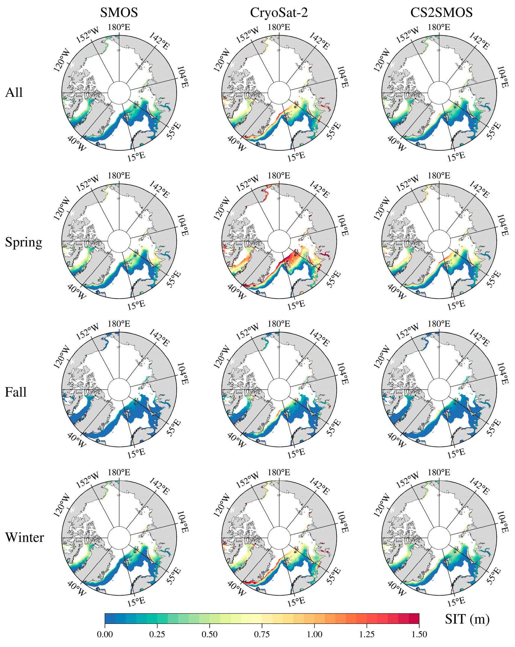
3.1.1. SMOS, CryoSat-2, and CS2SMOS over 2010–2023

During 2010–2023, the multi-year mean SIT measurements from SMOS, CryoSat-2, and CS2SMOS satellite data exhibited substantial concordance in the principal spatial distribution patterns (Figure 2). SMOS had the smallest mean SIT, with CryoSat-2 showing the largest mean SIT. Seasonal analyses further validated that the SIT rankings across spring (March–April), fall (October–November), and winter (December–February) matched the multi-year mean. In the seasonal ice zones, SMOS demonstrated better agreement with CS2SMOS than with CryoSat-2, as demonstrated by the lowest Bias, the lowest RMSE, and the highest CC observed between these two datasets (Figure 3).
During 2010–2023, the CC among the three satellite products was all very high, ranging from 0.80 to 0.94 (Figure 4). The highest CC was between SMOS and CS2SMOS, with their SIT values being the most similar. Time series analysis revealed that the mean SIT aligned with the multi-year spatial mean, confirming that SMOS had the smallest mean SIT, followed by CS2SMOS, with CryoSat-2 recording the largest SIT. The smallest SIT values for SMOS were generally observed in October, while CryoSat-2 and CS2SMOS sometimes recorded their smallest SIT in November. The largest SIT values for these three satellite products were typically observed in March and April, although occasionally the largest SIT values were observed in January or February. SMOS displayed a very slight declining trend in SIT, similar to CryoSat-2, while CS2SMOS showed a slight increasing trend, indicating minimal fluctuations in SIT within the seasonal ice zones.
The linear trend of the monthly average SIT data from October 2010 to April 2023 showed that, in terms of spatial distribution, all three satellite products revealed significant variations in SIT across the Atlantic region, particularly in regions such as the Greenland Sea, Barents Sea, and the Kara Sea (Figure 5). These variations were primarily characterized by a slight increasing trend. Notably, the SMOS product displayed more areas with pronounced SIT variations in the northern part of Baffin Bay compared to CS2 and CS2SMOS.

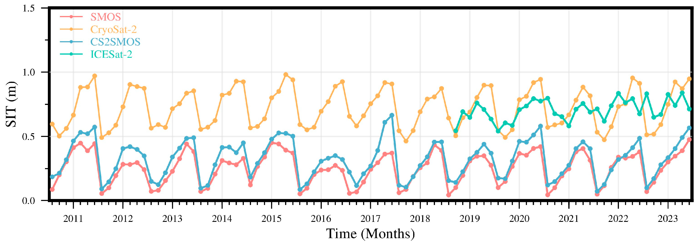
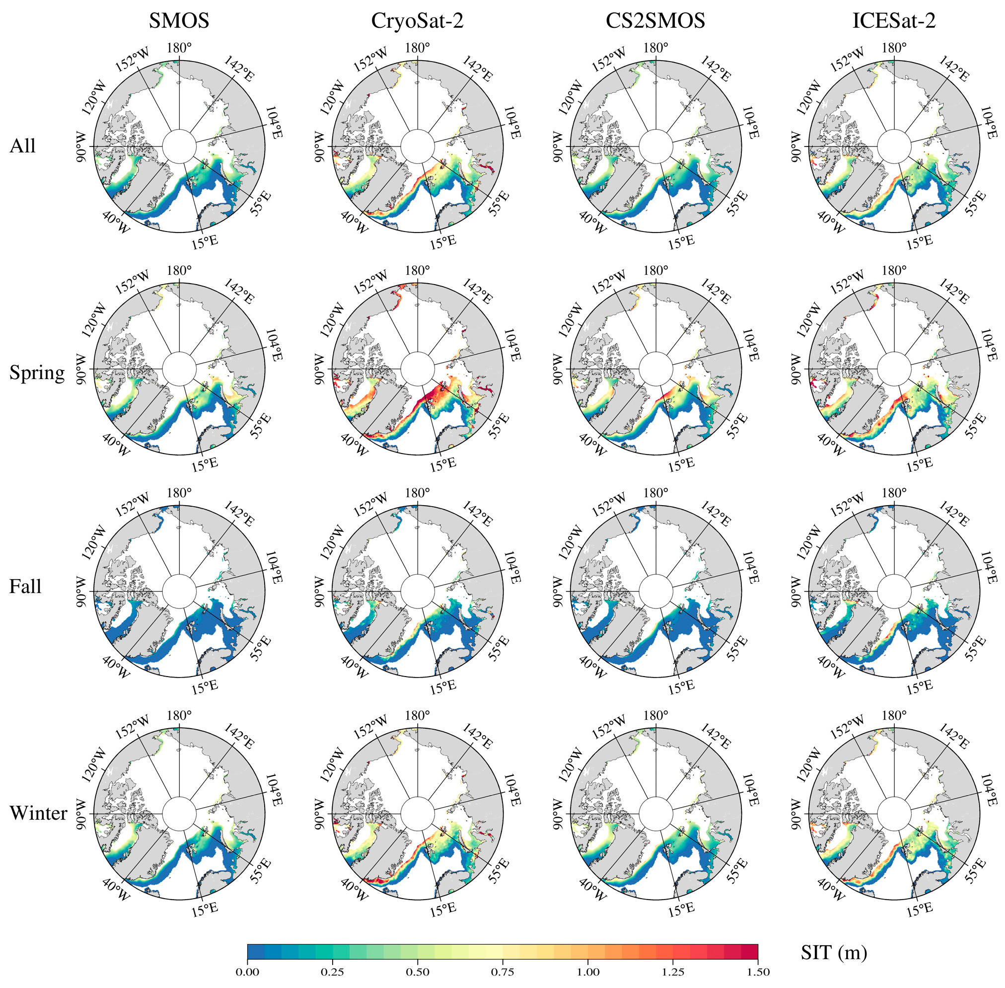
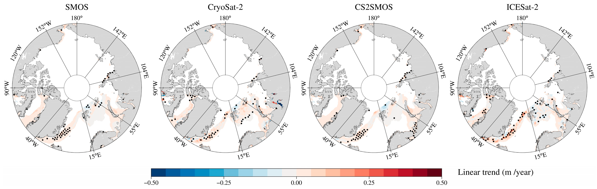
3.1.2. SMOS, CryoSat-2, CS2SMOS, and ICESat-2 over 2018–2023

Since the addition of ICESat-2 observations in 2018, intercomparisons of the multi-year mean spatial distribution of SIT revealed that SMOS had the smallest SIT values among the four sources. CryoSat-2 exhibited the largest SIT values, followed by ICESat-2 in second place and CS2SMOS in third (Figure 6). In spring and winter, the seasonal mean SIT from all four satellite products maintained the same ranking as the multi-year mean. However, in the fall, the seasonal mean SIT from ICESat-2 (0.135 m) was slightly higher than that from CryoSat-2 (0.131 m). According to the analysis of Bias, RMSE, and CC, the most significant similarity in the seasonal ice zones was between SMOS and CS2SMOS, followed by CryoSat-2 and CS2SMOS, with the consistency between ICESat-2 and CS2SMOS ranking third (Figure 3).
From 2018 to 2023, the pairwise CC between SMOS, CryoSat-2, and CS2SMOS products was relatively high (0.88–0.97), while the CC between ICESat-2 and the other three products was lower (0.37–0.46) (Figure 4). The CC between SMOS and CS2SMOS remained the highest among all products. Regarding SIT values, SMOS and CS2SMOS were closely aligned, while CryoSat-2 and ICESat-2 exhibited a similar alignment. The time series of mean SIT also indicated that SMOS recorded the smallest thickness values. CryoSat-2 exhibited the largest SIT, followed by ICESat-2 in second place and CS2SMOS in third. All four products exhibited very slight upward trends.
Further analysis of the spatial distribution of linear trends confirmed that in recent years, significant changes in SIT continued to be concentrated primarily in the Atlantic sector (Figure 7). All four satellite products indicated that slight upward trends in SIT mainly occurred in the Greenland Sea, while slight downward trends in SIT mainly occurred in the Barents Sea.

3.2. Evaluations of Multisource Satellite Data

The study of SIT intercomparisons allowed us to quantify the differences among various satellite datasets. Nevertheless, further evaluation using airborne and in situ observational data is necessary to clarify the performance of SMOS and other satellite datasets.

3.2.1. SMOS, CryoSat-2, and CS2SMOS over 2010–2023

During 2012–2013, an evaluation using OIB L4 data revealed that the three satellite products, SMOS, CryoSat-2, and CS2SMOS, generally underestimated SIT (Figure 8a). Among the three satellite products, CS2SMOS had the lowest DISO and was closest to OIB L4 (Table 1), with its CC (0.63) significantly higher than the other two products. While SMOS had the largest error with the highest DISO value due to the highest Bias and RMSE. Compared to SMOS, CryoSat-2 had a DISO closer to CS2SMOS, and it also had the lowest Bias and RMSE. Over the period 2012–2018, evaluations based on OIB Quick Look data demonstrated similarities with evaluations from OIB L4 data. Consistently, all three satellite products demonstrated a consistent tendency to underestimate the SIT when compared to the OIB Quick Look data (Figure 8b). In terms of DISO evaluation, SMOS exhibited the highest DISO value of 1.65, consistently showing the largest deviation from the OIB Quick Look (Table 1). CS2SMOS showed the lowest DISO at 1.09, closely followed by CryoSat-2 at 1.19. CS2SMOS also displayed the highest CC, indicating strong alignment with OIB Quick Look, while CryoSat-2 showed the lowest Bias and RMSE values.
Over the period 2011–2023, an evaluation was conducted on the Hall Beach station within the CAA station data. At Hall Beach, all three satellite products underestimated SIT (Figure 9). Based on DISO results, SMOS had the highest DISO of 1.64 with the lowest CC, indicating the greatest discrepancy (Table 1). In contrast, CryoSat-2 showed the lowest DISO.
Over the period 2013–2022, evaluations using ULS_BS data consistently revealed that all three satellite products underestimated SIT (Figure 10a). Regarding DISO evaluation, SMOS had the highest DISO, indicating the least accurate performance compared to CS2SMOS and CryoSat-2, which ranked first and second (Table 1). Among the three satellite products, SMOS showed the highest CC, while CryoSat-2 and CS2SMOS had the lowest Bias and RMSE, respectively. From 2010 to 2018, evaluations using ULS_FS data similarly indicated underestimations of SIT by all three satellite products (Figure 10b). CS2SMOS demonstrated the highest correlation coefficient, while CryoSat-2 exhibited the lowest Bias and RMSE. Overall, SMOS had the highest DISO, followed by CryoSat-2, while CS2SMOS had the lowest DISO (Table 1).
Based on a comprehensive evaluation spanning from 2010 to 2023 using data from OIB L4, OIB Quick Look, CAA station, ULS_BS, and ULS_FS, SMOS exhibited the weakest performance among the evaluated satellite products (Table 1), showing a large gap from what was expected in previous studies. In contrast, CS2SMOS demonstrated superior overall performance, closely followed by CryoSat-2, which exhibited performance comparable to CS2SMOS.

3.2.2. SMOS, CryoSat-2, CS2SMOS, and ICESat-2 over 2018–2023

In the evaluation incorporating ICESat-2 since 2018, only observational data from the CAA stations and ULS_BS were considered.
For the CAA station data, observations from the Hall Beach station were primarily concentrated in 2022, with smaller amounts in 2021 and 2023 (Figure 9). During the overlapping periods, SMOS had the highest DISO, while CryoSat-2 exhibited the lowest DISO (Table 1). SMOS, CS2SMOS, and ICESat-2 showed significant discrepancies compared to the CAA station data, primarily due to their higher Bias and RMSE, as well as lower CC, with correlations not being significant (p > 0.1).
From 2019 to 2022, in comparison to ULS_BS data, SMOS consistently underestimated SIT along with the other three satellite products (Figure 11). Despite SMOS showing the highest CC, it also displayed the highest Bias and RMSE values. In contrast, ICESat-2 exhibited the lowest Bias and RMSE. As a result, SMOS has the highest DISO, and ICESat-2 has the lowest DISO, indicating the consistency between ICESat-2 and ULS_BS data is closest (Table 1).
Based on a comprehensive evaluation spanning from 2018 to 2023, utilizing limited CAA station and ULS_BS data in specific locations and time frames, SMOS still displayed the largest discrepancies (Table 1). In contrast, ICESat-2 showcased the highest overall performance, followed closely by CryoSat-2, with CS2SMOS ranking third.

4. Discussion

In the evaluation of this study, the reference SIT data from ULS_BS and ULS_FS was not directly obtained but was inverted from sea ice draft. The uncertainty in the inversion method may affect the evaluation results. Currently, there are two primary methods for converting sea ice draft measurements obtained from ULS to SIT. The first method involves directly multiplying by a constant coefficient, with Fukamachi et al. [38] suggesting a coefficient range of 1.09 ± 0.05. This range reflects the potential variability in the conversion factor due to inherent uncertainties in the densities of sea ice (910 ± 20 kg/m3), snow (300 ± 100 kg/m3), and seawater (1025 kg/m3). The second method utilizes the hydrostatic balance equation (HBE) to calculate SIT [43]. Notably, the method requires snow depth and density data from the coupled product (SnowModel-LG_HS) [44] to retrieve SIT. Here, we designed a series of sensitivity experiments based on these two methods to retrieve different SIT evaluation data from two ULS datasets, and further discussed the impact of these two methods on evaluation results. Due to the time period limitations of the two ULS datasets and the data on snow depth and snow density used in the HBE, the sensitivity experiments focused on 2013–2022 for ULS_BS and 2010–2018 for ULS_FS in the evaluation of three satellite products. In the evaluation of four satellite products, the sensitivity experiments focused on 2018–2022 for ULS_BS.
The sensitivity results showed that in most cases, the rankings obtained from the two methods were consistent (Figure 12). In the evaluation of the three satellite products during the overlapping period, CS2SMOS generally performed the best, followed by CryoSat-2, with SMOS ranking third, which was consistent with the original evaluation results of this study. Only in the cases where the ULS_BS data were multiplied by 1.12–1.14, the ranking of CS2SMOS and CryoSat-2 was exchanged. In the evaluation of the four satellite products during the overlapping period, ICESat-2 always ranked first, CS2SMOS mostly second, CryoSat-2 third, and SMOS last, which was also consistent with the original evaluation result of this study. Only when the ULS_BS data were multiplied by 1.04–1.05 was the ranking of CS2SMOS and CryoSat-2 exchanged. It is important to note that the overestimation or underestimation of SIT due to the choice of conversion coefficient may result in differences in the performance of products such as CS2SMOS and CryoSat-2. However, overall, the results indicated that the thickness differences among different satellite products in seasonal ice zones are much greater than the differences derived from the evaluation data based on different coefficients. Therefore, the evaluation conclusions obtained using the original retrieval method have been shown to be robust based on the results of the sensitivity experiments.
Evaluating the SIT data from satellite products in the seasonal ice zones revealed that, despite updates to their versions, inconsistencies persisted in the SIT inversion outcomes among different satellites. These differences are mainly attributed to three factors [23,25]. Firstly, the sensor characteristics vary. SMOS measures sea ice brightness temperature using L-band microwave radiometry, which is sensitive to the dielectric properties of sea ice and can penetrate thin ice. CryoSat-2 uses a radar altimeter to measure radar freeboard. ICESat-2 utilizes a laser altimeter to measure total freeboard, which includes the thickness of snow on top of the sea ice. Secondly, the inversion algorithms used by the satellites differ. SMOS retrieves SIT based on brightness temperature, while CryoSat-2 and ICESat-2 derive SIT from freeboard data. Lastly, the determination of SIT in SMOS is influenced by the datasets used for ice salinity and sea ice concentration. In contrast, the inversion of SIT for CryoSat-2 and ICESat-2 is affected by differences in the choice of snow depth data and parameters for sea ice and snow density.
In addition, all four satellite products exhibited underestimation of SIT in seasonal ice zones, which are related to their respective uncertainties. For SMOS [28], snow cover in seasonal ice zones can insulate the ice and alter its thermal properties, leading to reduced observed brightness temperatures, which in turn results in underestimation of sea ice thickness. When sea ice concentration is below 100% or when ice salinity and temperature vary, the assumptions of uniform ice conditions and constant retrieval parameters may no longer hold. Under such conditions, the sensitivity of SMOS’s L-band signal to ice properties may decrease, thereby reducing the accuracy of SIT retrieval. For CryoSat-2 [29], surface roughness affects the leading-edge width of the radar echo, which in turn influences the accuracy of radar ranging and freeboard measurements. In seasonal ice zones, where the ice surface may be more irregular, variations in surface roughness can be more significant, further affecting measurement accuracy. Moreover, the snow depth models used for SIT estimation may not accurately reflect the actual snow conditions in seasonal ice zones, leading to uncertainties in the final SIT product. For ICESat-2 [31], laser signals can penetrate the snow layer, causing the measured freeboard height to be lower than the actual value, which results in an underestimation of sea ice thickness. The complex and variable distribution of snow in seasonal ice zones introduces further uncertainties in the estimation of snow depth and density, thereby affecting the accuracy of SIT retrieval. For CS2SMOS [19], the OI scheme helps compensate for some shortcomings of single satellite data, but limitations still remain. In seasonal ice zones, uncertainties in the background field and insufficient observational weighting constrain the accurate estimation of SIT.
It is worth noting that recent advancements in spaceborne GNSS-Reflectometry (GNSS-R) have shown promise in sea ice thickness retrieval. Recent studies utilizing Fengyun-3E (FY-3E) data have demonstrated the potential of GNSS-R to provide high-resolution, all-weather measurements [45,46], which can be particularly beneficial for sea ice thickness retrieval in seasonal ice zones where traditional microwave and radar techniques face limitations. Given the limitations of SMOS identified in this study, future research could focus on integrating GNSS-R data with current satellite missions, such as SMOS and CryoSat-2, to improve the accuracy, spatial coverage, and reliability of sea ice thickness retrievals, particularly in regions with thin ice or other challenging observational conditions.
Furthermore, the evaluation results are affected by the observation period of the satellite products and the selection of evaluation data. In this study, the evaluation results can only represent the performance of satellite products during the freezing season, as the time range of observation data is only from October to April. However, the performance of satellite products from May to September is still unclear. In addition, due to the limited evaluation data in the seasonal ice zones, the evaluation results of this study can only represent the performance of satellite products in the region where the evaluation data are available. Therefore, it is necessary to introduce more evaluation data in the future for further evaluations.

5. Conclusions

Currently, the quantified performance of SMOS retrieval accuracy in Arctic average thin ice thickness below 0.5 m compared with other satellite products is still unclear. This study provides the first evaluation of SMOS performance over the period 2010–2023. The latest versions of CryoSat-2, CS2SMOS, and ICESat-2 satellite products were incorporated for comparison as reference datasets. Given the availability of ICESat-2 satellite data since 2018, the study segments the intercomparison and evaluation of satellite data into two periods: 2010–2023 and 2018–2023.
During 2010–2023, the multi-year mean SIT data collected by SMOS, CryoSat-2, and CS2SMOS exposed similarities in the spatial distribution in the seasonal ice zones. Among these satellite products, SMOS exhibited the smallest mean SIT, while CryoSat-2 had the largest mean SIT. In the seasonal ice zones, SMOS showed greater SIT consistency with CS2SMOS compared to CryoSat-2. Monthly variations in the SIT time series between SMOS, CryoSat-2, and CS2SMOS showed strong correlations. SMOS and CryoSat-2 displayed a slight downward trend, whereas CS2SMOS indicated a slight upward trend over time.
In the period from 2018 to 2023, the mean SIT retrieved from SMOS was the smallest among the satellite products. CryoSat-2 exhibited the largest SIT values, followed by ICESat-2 in second place and CS2SMOS in third. SMOS exhibited the highest similarity with CS2SMOS, followed by CryoSat-2 and CS2SMOS, while ICESat-2 showed the lowest consistency with CS2SMOS. ICESat-2 showed lower correlation with SMOS, CryoSat-2, and CS2SMOS. Additionally, all four products demonstrated a slight upward trend over the period studied.
Based on evaluations using various datasets from airborne and in situ measurements, it was evident that the four satellite products generally underestimated SIT in the seasonal ice zones. SMOS consistently exhibited the weakest performance across both selected periods, which showed a large gap from what was expected in previous studies. In contrast, CS2SMOS showed the strongest agreement with evaluation datasets including OIB L4, OIB Quick Look, CAA-Station, ULS_BS, and ULS_FS during 2010–2023. Therefore, the overall evaluation results highlighted CS2SMOS as the satellite product with the best overall performance. Similarly, ICESat-2 showed the best overall performance from 2018 to 2023, demonstrating the closest agreement with the CAA station and ULS_BS datasets.
The previous knowledge suggested that SMOS exhibited higher accuracy in seasonal ice zones with SIT below 0.5 m. However, this study is the first to reveal a completely different conclusion, showing that SMOS demonstrates the weakest performance in seasonal ice zones compared to CryoSat-2, CS2SMOS, and ICESat-2. Additionally, this study deepens the understanding of the SIT variation in the seasonal ice zones and clarifies the performance and differences in various satellite products in this area. The findings will help improve the inversion of satellite products in the future and potentially enhance the reliability of Arctic sea ice observations.

Author Contributions

Conceptualization, Y.Z. (Yu Zhang) and C.C.; methodology, H.L., J.L. and Y.Z. (Yi Zhou); software, H.L.; validation, H.G., W.S. and D.W.; formal analysis, H.L. and J.L.; data curation, S.H.; writing—original draft preparation, H.L., J.L. and Y.Z. (Yu Zhang); writing—review and editing, H.G., C.C. and Y.Z. (Yi Zhou); visualization, H.L. and J.L.; supervision, Y.Z. (Yu Zhang) and H.G. All authors have read and agreed to the published version of the manuscript.

Funding

This work is sponsored by the National Natural Science Foundation of China (No. 42376231 and No. 42130402), National Key Research and Development Program of China (No. 2019YFA0607001), Natural Science Foundation of Shanghai (No. 22ZR1427400), and Artificial Intelligence Research Program of Shanghai Municipal Education Commission (No. A1-3405-25-000302).

Data Availability Statement

The SMOS SIT data are available at ftp://ftp.awi.de/sea_ice/product/smos/v3.3/nh/ (accessed on 7 May 2025). The CryoSat-2 SIT data can be downloaded at ftp://ftp.awi.de/sea_ice/product/cryosat2/v2p6/nh/l3c_grid/month/ (accessed on 7 May 2025). The CS2SMOS SIT data are available at ftp://ftp.awi.de/sea_ice/product/cryosat2_smos/v206/nh/ (accessed on 7 May 2025). The ICESat-2 SIT data can be collected at https://nsidc.org/data/is2sitmogr4/versions/3 (accessed on 7 May 2025). The OIB L4 SIT data can be obtained at https://nsidc.org/data/idcsi4/versions/1 (accessed on 7 May 2025). The OIB Quick Look SIT data can be downloaded at https://nsidc.org/data/nsidc-0708/versions/1 (accessed on 7 May 2025). The CAA station SIT data can be collected at https://data-donnees.az.ec.gc.ca/data/ice/products/ice-thickness-program-collection/?lang=en (accessed on 7 May 2025). The sea ice draft data in the Barents Sea is available at https://zenodo.org/records/10986370 (accessed on 7 May 2025). The sea ice draft data in Fram Strait can be downloaded at https://data.npolar.no/dataset/5b717274-2d85-4f13-a1b4-ff0517c78b4a (accessed on 7 May 2025). The snow depth and snow density data of SnowModel-LG_HS can be obtained at https://fmi.b2share.csc.fi/records/e4b0307d7dc74b449d03a41b6cae65d8 (accessed on 7 May 2025).

Acknowledgments

We thank all the scientists who contributed to the multi-source datasets used in this study. We would also like to express our sincere gratitude to the editor and anonymous reviewers for their constructive comments.

Conflicts of Interest

The authors declare no conflicts of interest.

References

  1. Serreze, M.C.; Barrett, A.P.; Slater, A.G.; Woodgate, R.A.; Aagaard, K.; Lammers, R.B.; Steele, M.; Moritz, R.; Meredith, M.; Lee, C.M. The large-scale freshwater cycle of the Arctic. J. Geophys. Res. Ocean. 2006, 111, C11010. [Google Scholar] [CrossRef]
  2. Coachman, L.K.; Aagaard, K. Transports through Bering Strait: Annual and interannual variability. J. Geophys. Res. Ocean. 1988, 93, 15535–15539. [Google Scholar] [CrossRef]
  3. Fahrbach, E.; Meincke, J.; Østerhus, S.; Rohardt, G.; Schauer, U.; Tverberg, V.; Verduin, J. Direct measurements of volume transports through Fram Strait. Polar Res. 2001, 20, 217–224. [Google Scholar] [CrossRef]
  4. Rothrock, D.A.; Percival, D.B.; Wensnahan, M. The decline in arctic sea-ice thickness: Separating the spatial, annual, and interannual variability in a quarter century of submarine data. J. Geophys. Res. Ocean. 2008, 113, C05003. [Google Scholar] [CrossRef]
  5. Lindsay, R.; Schweiger, A. Arctic sea ice thickness loss determined using subsurface, aircraft, and satellite observations. Cryosphere 2015, 9, 269–283. [Google Scholar] [CrossRef]
  6. Kwok, R. Arctic sea ice thickness, volume, and multiyear ice coverage: Losses and coupled variability (1958–2018). Environ. Res. Lett. 2018, 13, 105005. [Google Scholar] [CrossRef]
  7. Kacimi, S.; Kwok, R. Arctic snow depth, ice thickness, and volume from ICESat-2 and CryoSat-2: 2018–2021. Geophys. Res. Lett. 2022, 49, e2021GL097448. [Google Scholar] [CrossRef]
  8. Wang, K.; Zhang, Y.; Chen, C.; Song, S.; Chen, Y. Impacts of Arctic Sea Fog on the Change of Route Planning and Navigational Efficiency in the Northeast Passage during the First Two Decades of the 21st Century. J. Mar. Sci. Eng. 2023, 11, 2149. [Google Scholar] [CrossRef]
  9. Zhang, Y.; Sun, X.; Zha, Y.; Wang, K.; Chen, C. Changing arctic northern sea route and transpolar sea route: A prediction of route changes and navigation potential before Mid-21st century. J. Mar. Sci. Eng. 2023, 11, 2340. [Google Scholar] [CrossRef]
  10. Haas, C.; Gerland, S.; Eicken, H.; Miller, H. Comparison of sea-ice thickness measurements under summer and winter conditions in the Arctic using a small electromagnetic induction device. Geophysics 1997, 62, 749–757. [Google Scholar] [CrossRef]
  11. Rothrock, D.A.; Wensnahan, M. The accuracy of sea ice drafts measured from US Navy submarines. J. Atmos. Ocean. Technol. 2007, 24, 1936–1949. [Google Scholar] [CrossRef]
  12. Richter-Menge, J.A.; Perovich, D.K.; Elder, B.C.; Claffey, K.; Rigor, I.; Ortmeyer, M. Ice mass-balance buoys: A tool for measuring and attributing changes in the thickness of the Arctic sea-ice cover. Ann. Glaciol. 2006, 44, 205–210. [Google Scholar] [CrossRef]
  13. Kurtz, N.T.; Farrell, S.L.; Studinger, M.; Galin, N.; Harbeck, J.P.; Lindsay, R.; Onana, V.D.; Panzer, B.; Sonntag, J.G. Sea ice thickness, freeboard, and snow depth products from Operation IceBridge airborne data. Cryosphere 2013, 7, 1035–1056. [Google Scholar] [CrossRef]
  14. Pfaffling, A.; Haas, C.; Reid, J.E. Direct helicopter EM—Sea-ice thickness inversion assessed with synthetic and field data. Geophysics 2007, 72, F127–F137. [Google Scholar] [CrossRef]
  15. Markus, T.; Neumann, T.; Martino, A.; Abdalati, W.; Brunt, K.; Csatho, B.; Farrell, S.; Fricker, H.; Gardner, A.; Harding, D. The Ice, Cloud, and land Elevation Satellite-2 (ICESat-2): Science requirements, concept, and implementation. Remote Sens. Environ. 2017, 190, 260–273. [Google Scholar] [CrossRef]
  16. Zwally, H.J.; Schutz, B.; Abdalati, W.; Abshire, J.; Bentley, C.; Brenner, A.; Bufton, J.; Dezio, J.; Hancock, D.; Harding, D. ICESat’s laser measurements of polar ice, atmosphere, ocean, and land. J. Geodyn. 2002, 34, 405–445. [Google Scholar] [CrossRef]
  17. Laxon, S.W.; Giles, K.A.; Ridout, A.L.; Wingham, D.J.; Willatt, R.; Cullen, R.; Kwok, R.; Schweiger, A.; Zhang, J.; Haas, C. CryoSat-2 estimates of Arctic sea ice thickness and volume. Geophys. Res. Lett. 2013, 40, 732–737. [Google Scholar] [CrossRef]
  18. Mecklenburg, S.; Drusch, M.; Kerr, Y.H.; Font, J.; Martin-Neira, M.; Delwart, S.; Buenadicha, G.; Reul, N.; Daganzo-Eusebio, E.; Oliva, R. ESA’s soil moisture and ocean salinity mission: Mission performance and operations. IEEE Trans. Geosci. Remote Sens. 2012, 50, 1354–1366. [Google Scholar] [CrossRef]
  19. Ricker, R.; Hendricks, S.; Kaleschke, L.; Tian-Kunze, X.; King, J.; Haas, C. A weekly Arctic sea-ice thickness data record from merged CryoSat-2 and SMOS satellite data. Cryosphere 2017, 11, 1607–1623. [Google Scholar] [CrossRef]
  20. Li, M.; Ke, C.Q.; Xie, H.; Miao, X.; Shen, X.; Xia, W. Arctic sea ice thickness retrievals from CryoSat-2: Seasonal and interannual comparisons of three different products. Int. J. Remote Sens. 2020, 41, 152–170. [Google Scholar] [CrossRef]
  21. Petty, A.A.; Kurtz, N.T.; Kwok, R.; Markus, T.; Neumann, T.A. Winter Arctic sea ice thickness from ICESat-2 freeboards. J. Geophys. Res. Ocean. 2020, 125, e2019JC015764. [Google Scholar] [CrossRef]
  22. Sallila, H.; Farrell, S.L.; McCurry, J.; Rinne, E. Assessment of contemporary satellite sea ice thickness products for Arctic sea ice. Cryosphere 2019, 13, 1187–1213. [Google Scholar] [CrossRef]
  23. Soriot, C.; Prigent, C.; Jimenez, C.; Frappart, F. Arctic sea ice thickness estimation from passive microwave satellite observations between 1.4 and 36 GHz. Earth Space Sci. 2023, 10, e2022EA002542. [Google Scholar] [CrossRef]
  24. Zhou, Y.; Zhang, Y.; Chen, C.; Li, L.; Xu, D.; Beardsley, R.C.; Shao, W. Assessment of radar freeboard, radar penetration rate, and snow depth for potential improvements in Arctic sea ice thickness retrieved from CryoSat-2. Cold Reg. Sci. Technol. 2025, 231, 104408. [Google Scholar] [CrossRef]
  25. Tian-Kunze, X.; Kaleschke, L.; Maaß, N.; Mäkynen, M.; Serra, N.; Drusch, M.; Krumpen, T. SMOS-derived thin sea ice thickness: Algorithm baseline, product specifications and initial verification. Cryosphere 2014, 8, 997–1018. [Google Scholar] [CrossRef]
  26. Tietsche, S.; Alonso-Balmaseda, M.; Rosnay, P.; Zuo, H.; Tian-Kunze, X.; Kaleschke, L. Thin Arctic sea ice in L-band observations and an ocean reanalysis. Cryosphere 2018, 12, 2051–2072. [Google Scholar] [CrossRef]
  27. Chen, F.; Wang, D.; Zhang, Y.; Zhou, Y.; Chen, C. Intercomparisons and evaluations of satellite-derived arctic sea ice thickness products. Remote Sens. 2024, 16, 508. [Google Scholar] [CrossRef]
  28. Kaleschke, L.; Tian-Kunze, X.; Maaß, N.; Mäkynen, M.; Drusch, M. Sea ice thickness retrieval from SMOS brightness temperatures during the Arctic freeze-up period. Geophys. Res. Lett. 2012, 39, L05501. [Google Scholar] [CrossRef]
  29. Ricker, R.; Hendricks, S.; Helm, V.; Skourup, H.; Davidson, M. Sensitivity of CryoSat-2 Arctic sea-ice freeboard and thickness on radar-waveform interpretation. Cryosphere 2014, 8, 1607–1622. [Google Scholar] [CrossRef]
  30. Warren, S.G.; Rigor, I.G.; Untersteiner, N.; Radionov, V.F.; Bryazgin, N.N.; Aleksandrov, Y.I.; Colony, R. Snow depth on Arctic sea ice. J. Clim. 1999, 12, 1814–1829. [Google Scholar] [CrossRef]
  31. Petty, A.A.; Kurtz, N.T.; Kwok, R.; Markus, T.; Neumann, T.A.; Keeney, N. ICESat-2 L4 Monthly Gridded Sea Ice Thickness, Version 3; NASA National Snow and Ice Data Center Distributed Active Archive Center: Boulder, CO, USA, 2023. [Google Scholar] [CrossRef]
  32. Petty, A.A.; Webster, M.; Boisvert, L.; Markus, T. The NASA Eulerian Snow on Sea Ice Model (NESOSIM) v1. 0: Initial model development and analysis. Geosci. Model Dev. 2018, 11, 4577–4602. [Google Scholar] [CrossRef]
  33. Kurtz, N.; Studinger, M.; Harbeck, J.; Onana, V.; Yi, D. IceBridge L4 Sea Ice Freeboard, Snow Depth, and Thickness, Version 1; NASA National Snow and Ice Data Center Distributed Active Archive Center: Boulder, CO, USA, 2015. [Google Scholar] [CrossRef]
  34. Kurtz, N.; Studinger, M.; Harbeck, J.; Onana, V.; Yi, D. IceBridge Sea Ice Freeboard, Snow Depth, and Thickness Quick Look, Version 1; NASA National Snow and Ice Data Center Distributed Active Archive Center: Boulder, CO, USA, 2016. [Google Scholar] [CrossRef]
  35. Hansen, E.; Ervik, Å.; Eik, K.; Olsson, A.; Teigen, S.H. Long-term observations (2014–2020) of level ice draft, keel depth and ridge frequency in the Barents Sea. Cold Reg. Sci. Technol. 2023, 216, 103988. [Google Scholar] [CrossRef]
  36. Fissel, D.B.; Marko, J.R.; Melling, H. Advances in upward looking sonar technology for studying the processes of change in Arctic Ocean ice climate. J. Oper. Oceanogr. 2008, 1, 9–18. [Google Scholar] [CrossRef]
  37. Melling, H.; Johnston, P.H.; Riedel, D.A. Measurements of the underside topography of sea ice by moored subsea sonar. J. Atmos. Ocean. Technol. 1995, 12, 589–602. [Google Scholar] [CrossRef]
  38. Fukamachi, Y.; Simizu, D.; Ohshima, K.I.; Eicken, H.; Mahoney, A.R.; Iwamoto, K.; Moriya, E.; Nihashi, S. Sea-ice thickness in the coastal northeastern Chukchi Sea from moored ice-profiling sonar. J. Glaciol. 2017, 63, 888–898. [Google Scholar] [CrossRef]
  39. Sumata, H.; Divine, D.; de Steur, L. Monthly Mean Sea Ice Draft from the Fram Strait Arctic Outflow Observatory Since 1990; Norwegian Polar Institute: Tromsø, Norway, 2021. [Google Scholar] [CrossRef]
  40. Kwok, R.; Cunningham, G.F. Variability of Arctic sea ice thickness and volume from CryoSat-2. Philos. Trans. R. Soc. A Math. Phys. Eng. Sci. 2015, 373, 20140157. [Google Scholar] [CrossRef] [PubMed]
  41. Hu, Z.; Chen, D.; Chen, X.; Zhou, Q.; Peng, Y.; Li, J.; Sang, Y. CCHZ-DISO: A timely new assessment system for data quality or model performance from Da Dao Zhi Jian. Geophys. Res. Lett. 2022, 49, e2022GL100681. [Google Scholar] [CrossRef]
  42. Zhang, Y.; Li, G.; Li, H.; Chen, C.; Shao, W.; Zhou, Y.; Wang, D. A Spatiotemporal Comparison and Assessment of Multisource Satellite Derived Sea Ice Thickness in the Arctic Thinner Ice Region. IEEE J. Sel. Top. Appl. Earth Obs. Remote Sens. 2024, 17, 8710–8723. [Google Scholar] [CrossRef]
  43. Bourke, R.H.; Paquette, R.G. Estimating the thickness of sea ice. J. Geophys. Res. Ocean. 1989, 94, 919–923. [Google Scholar] [CrossRef]
  44. Merkouriadi, I.; Liston, G. Quantifying Pan-Arctic Snow Depth and Density Trends Caused by Snow-Ice Formation; Finnish Meteorological Institute: Helsinki, Finland, 2023. [Google Scholar] [CrossRef]
  45. Xie, Y.; Yan, Q. Stand-alone retrieval of sea ice thickness from FY-3E GNOS-R data. IEEE Geosci. Remote Sens. Lett. 2024, 21, 2000305. [Google Scholar] [CrossRef]
  46. Xie, Y.; Yan, Q. Retrieval of sea ice thickness using FY-3E/GNOS-II data. Satell. Navig. 2024, 5, 17. [Google Scholar] [CrossRef]
Figure 1. The distribution of evaluation data and the division of the Arctic seasonal ice zones into several subregions: Chukchi Sea, Laptev Sea, Kara Sea, Barents Sea, Greenland Sea, and Baffin Island. The defined seasonal ice zones are represented by blue shading.
Remotesensing 17 01680 g001
Figure 2. Spatial distribution of multi-year mean SIT and seasonal mean SIT for SMOS, CryoSat-2, and CS2SMOS during 2010–2023.
Remotesensing 17 01680 g002
Figure 3. Bias, RMSE, and CC of SIT among satellite products, based on monthly spatial samples spanning 2010–2023 and 2018–2023. Bias quantifies the discrepancy between the Y-axis and X-axis satellite products.
Remotesensing 17 01680 g003
Figure 4. Monthly variations in spatial mean SIT for SMOS, CryoSat-2, CS2SMOS, and ICESat-2 during 2010–2023.
Remotesensing 17 01680 g004
Figure 5. Linear trend of SIT for SMOS, CryoSat-2, and CS2SMOS from 2010 to 2023. The black dots represent the regression slopes with a 95% confidence interval.
Remotesensing 17 01680 g005
Figure 6. Spatial distribution of multi-year mean SIT and seasonal mean SIT for SMOS, CryoSat-2, CS2SMOS, and ICESat-2 during 2018–2023.
Remotesensing 17 01680 g006
Figure 7. Linear trend of SIT for SMOS, CryoSat-2, CS2SMOS, and ICESat-2 from 2018 to 2023. The black dots represent the regression slopes with a 95% confidence interval.
Remotesensing 17 01680 g007
Figure 8. Evaluation of satellite SIT retrieved from SMOS, CryoSat-2, and CS2SMOS using (a) OIB L4 and (b) OIB Quick Look. The solid black line indicates the best fit line, and the dashed line indicates the scatter fit line.
Remotesensing 17 01680 g008
Figure 9. Evaluation of satellite SIT retrieved from SMOS, CryoSat-2, CS2SMOS, and ICESat-2 using the CAA station data.
Remotesensing 17 01680 g009
Figure 10. Evaluation of satellite SIT retrieved from SMOS, CryoSat-2, and CS2SMOS using (a) ULS_BS and (b) ULS_FS data. The solid black line indicates the best fit line, and the dashed line indicates the scatter fit line.
Remotesensing 17 01680 g010
Figure 11. Evaluation of satellite SIT retrieved from SMOS, CryoSat-2, CS2SMOS, and ICESat-2 using ULS_BS data. The solid black line indicates the best fit line, and the dashed line indicates the scatter fit line.
Remotesensing 17 01680 g011
Figure 12. The sensitivity experiments of DISO values for (a) ULS_BS data from 2013 to 2022, (b) ULS_BS data from 2018 to 2022, and (c) ULS_FS data from 2010 to 2018.
Remotesensing 17 01680 g012
Table 1. DISO values for satellite retrieved SIT based on various evaluation datasets.
2010−20232018−2023
SMOSCryoSat-2CS2SMOSSMOSCryoSat-2CS2SMOSICESat-2
OIB L41.63851.37861.2145////
OIB Quick Look1.65731.19391.0958////
CAA station1.64781.16131.64891.65151.19061.60731.5605
ULS_BS1.48101.39911.39011.49471.41831.44501.2041
ULS_FS1.49761.12320.8227////
Overall performance1.66601.26071.20521.51271.39831.48131.3228
Disclaimer/Publisher’s Note: The statements, opinions and data contained in all publications are solely those of the individual author(s) and contributor(s) and not of MDPI and/or the editor(s). MDPI and/or the editor(s) disclaim responsibility for any injury to people or property resulting from any ideas, methods, instructions or products referred to in the content.

