Abstract
Cloud detection in satellite imagery plays a pivotal role in achieving high-accuracy retrieval of biophysical parameters and subsequent remote sensing applications. Although numerous methods have been developed and operationally deployed, their accuracy over challenging surfaces—such as snow-covered mountains, saline–alkali lands in deserts or Gobi regions, and snow-covered surfaces—remains limited. Additionally, the efficiency of collecting training samples for prevalent deep learning-based methods heavily relies on large-scale pixel-level annotations, which are both time-consuming and labor-intensive. To address these challenges, we propose a Texture-Enhanced Network that integrates an object-oriented dynamic threshold pseudo-labeling method and a texture-feature-enhanced attention module to enhance both the efficiency of deep learning methods and detection accuracy over challenging surfaces. First, an object-oriented dynamic threshold pseudo-labeling approach is developed by leveraging object-oriented principles and adaptive thresholding techniques, enabling the efficient collection of large-scale labeled samples for challenging surfaces. Second, to exploit the spatial continuity of clouds, cross-channel correlations, and their distinctive texture features, a texture-feature-enhanced attention module is designed to improve feature discrimination for challenging positive and negative samples. Extensive experiments on a Chinese GaoFen satellite imagery dataset demonstrate that the proposed method achieves state-of-the-art performance.
1. Introduction
With the development of remote sensing (RS) technology, an increasing amount of satellite data has become available, and optical RS imagery provides the most direct visual experience. Many existing studies are based on optical RS imagery, such as environmental and disaster monitoring [1], climate change research [2], agricultural production [3], and urban management planning [4]. However, according to the International Satellite Cloud Climatology Project (ISCCP) global cloud coverage data, clouds cover about 55% of land and 72% of oceans [5], making cloud pixels an inevitable component of optical RS imagery. Based on the sensor imaging mechanism, multispectral RS imagery first encounters cloud and fog information during data transmission. The ground object information beneath the clouds is often distorted due to the absorption, reflection, and re-radiation of various radiation energies by the cloud layer, leading to blurred textures or even complete loss of texture information. On one hand, clouds are important meteorological elements, and weather forecasting [6] and related climate change research require cloud data. On the other hand, cloud cover can block or reflect sunlight, potentially causing spatial discontinuities in RS data. In some regions, RS data may be difficult to acquire or of lower quality, affecting the retrieval and quality of RS imagery, and subsequently impacting further research. Therefore, accurately distinguishing cloud pixels, or cloud detection, is an indispensable part of RS data processing. It plays a decisive role in improving the quality and scope of RS data and promotes the use of RS imagery in various applications. For example, in land cover classification, regions contaminated by clouds need to be excluded in advance to obtain more accurate results [7].
The goal of cloud detection in optical RS imagery is to separate cloud pixels from background pixels. Currently, cloud detection in optical RS imagery has been widely studied, and many methods have been proposed [8]. Four primary categories of cloud detection methods exist:
- (1)
- Traditional threshold-based and texture analysis-based image processing methods, which primarily rely on analyzing the spectral characteristics of clouds and other objects in the image. These methods set different thresholds for various spectral channels in RS imagery to detect clouds. However, they face challenges with issues such as large areas of bright ground surfaces and snow being misclassified as clouds [9].
- (2)
- Machine learning methods based on handcrafted physical features use manually selected features such as image texture and brightness. These methods demonstrate good detection accuracy and robustness but exhibit lower accuracy when detecting thin clouds compared to thick clouds [10].
- (3)
- Deep learning methods based on convolutional neural networks have been widely used for cloud detection and have achieved excellent performance [8]. These methods design different network architectures to extract hierarchical features for cloud detection. However, most of these methods require large, precise, pixel-level annotated datasets, which are time-consuming and expensive to create due to the diverse types of clouds and their irregular geometric structures and uneven spectral characteristics.
- (4)
- Weakly supervised cloud detection (WDCD) methods have gained widespread attention to address the annotation burden. However, these methods’ performance based on physical properties is not ideal in complex cloud scenes and mixed ice/snow environments. Since the training samples are scarce for these challenging surfaces, the WDCD methods have low accuracy for certain specific scenes, such as snow-covered mountains, snow-covered land, deserts, saline–alkali land, and urban bright surfaces, as shown in Figure 1. As a result, weakly supervised deep learning (DL) models trained on these inaccurate datasets often produce poor predictions in such scenes.
Optical and multispectral remote sensing systems capture Earth’s surface reflectance across visible (VIS), near-infrared (NIR), and shortwave infrared (SWIR) bands, with spatial resolutions ranging from sub-meter to kilometers. Landsat 8/9 provides 11 spectral bands, including SWIR (1.57–2.29 µm) and thermal infrared, at a 30 m resolution. Sentinel-2A/B offers 13 bands at 10 m (VIS/NIR), 20 m (red-edge, SWIR), and 60 m resolutions, emphasizing red-edge (0.705–0.783 µm) for vegetation and coastal analysis. MODIS covers 36 bands (0.4–14.4 µm) at 250 m (VIS/NIR), 500 m (SWIR), and 1km resolutions, prioritizing broad-scale climate and aerosol studies. China’s GaoFen (GF) series (GF-1/2/6) features multispectral bands (2–8 m) and panchromatic sensors (0.8–2 m), with GF-6 integrating red-edge bands (0.71–0.89 µm) for agricultural monitoring. Landsat and Sentinel-2 balance spectral diversity and moderate resolution for environmental tracking, while MODIS trades spatial detail for daily global coverage. GF targets regional precision with high-resolution, application-specific bands.
Another challenge for our research on GF RS images is the absence of thermal–infrared and SWIR bands; unlike ACCA [11] and Fmask [12] algorithms designed based on Landsat and Sentinel-2, we cannot utilize temperature data to improve the accuracy of cloud detection over bare ground, artificial surfaces, or ice and snow scenes. To address these issues, we propose a novel WDCD framework based on an adaptive object-oriented method. Firstly, based on Zhong’s method [13], the framework adaptively generates rough high-confidence and low-confidence cloud masks using physical rules. By utilizing the affine invariance relationship between clouds and cloud shadows, some misdetections are effectively filtered out, resulting in RS imagery and corresponding samples that are satisfactory with sufficient quality for training. Inspired by Haar wavelet downsampling (HWD) [14], we design a plug-and-play downsampling module based on these inaccurate supervision data, which strengthens the learning of cloud texture, spatial, and channel features in the image.
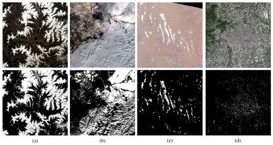
Figure 1.
The first row displays the RS imagery, and the second row presents the generated cloud masks. The cloud mask is derived from an enhanced ACCA algorithm [13]. (a) is a snow-covered mountain scene, where the bright snow-covered mountain is incorrectly classified as cloud; (b) is a snow-covered scene, where the snow-covered areas are incorrectly classified as cloud; (c) is a desert saline–alkali land scene; (d) is an urban scene, where the clearly identifiable urban area in the RS imagery is still incorrectly classified as cloud.
The contributions of this work are summarized as follows:
- (1)
- We develop an adaptive, object-oriented framework with hybrid attention mechanisms for WDCD.
- (2)
- We propose an automated method to generate large-scale pseudo-cloud annotations without human intervention, significantly improving efficiency while substantially increasing sample acquisition for the challenging surfaces.
- (3)
- A downsampling module utilizing Haar wavelet transformation is designed to strengthen multi-dimensional attention mechanisms (textural, spatial, and channel-wise) through learning complex cloud features, enabling accurate identification of thin cloud regions with subtle spectral characteristics while excluding bright backgrounds.
- (4)
- Extensive experiments using the four-band GF-1 dataset demonstrate the method’s effectiveness. The remainder of this paper is organized as follows: Section 2 reviews related work; Section 3 details the proposed framework; Section 4 presents the GF-1 dataset and experimental analysis; Section 5 concludes with a summary of key findings and discusses potential directions for future improvements.
2. Related Work
This section presents a concise overview of related work, encompassing cloud detection in RS imagery, and wavelet transform and feature enhancement methods in image processing.
2.1. Cloud Detection in RS Imagery
Physics-based methods leverage the physical characteristics of clouds for detection. Representative cloud detection algorithms include the Automated Cloud Cover Assessment (ACCA) algorithm. The ACCA algorithm establishes threshold rules based on the physical characteristics of clouds and shadows for detection, using 5 bands with 26 band-specific test rules. This method demonstrates operational efficiency and exhibits minimal systematic bias [11]. The Multi-Feature Combined (MFC) automatic cloud and shadow detection algorithm improves detection accuracy in cloud and cloud shadow edge regions by using guided filtering [15]. Zhong et al. modified the traditional ACCA method for GF-1 WFV data, converting clouds and shadows into cloud and shadow objects, and through object-oriented matching, eliminated unreasonable objects, achieving an overall accuracy of cloud detection close to 90% [13].
Traditional methods relying on manual physical feature selection and classical machine learning models (e.g., Support Vector Machines (SVMs) and Random Forests) for image block/pixel classification have been extensively utilized in cloud detection. For example, Tian et al. developed a cloud detection method that utilized a gray-level co-occurrence matrix (GLCM) to extract texture features and then trained a nonlinear SVM to segment clouds [16].
In recent years, DL methods have demonstrated significant advancements and maturation in image detection and recognition domains, leading to widespread adoption of DL techniques for RS imagery cloud detection among researchers worldwide. These approaches have progressively outperformed conventional cloud detection algorithms that rely on physical characteristics. Li et al. integrated multi-scale spectral and spatial features into a lightweight cloud detection network, using mixed-depth separable convolutions and shared and dilated residual blocks to effectively merge spectral and spatial features. This approach is computationally efficient and does not introduce additional parameters [17].
Accurate differentiation between high-reflectance snow-covered regions and cloud-covered areas continues to pose a significant challenge in cloud detection research. Zhang et al. proposed a cloud detection method based on cascaded feature attention and channel attention CNNs to enhance attention on color and texture features [18]. They employed dilated convolutions to emphasize important information in the channel dimension and used dilated convolutions with different dilation rates to capture information from multiple receptive fields. Wu et al. incorporated geographic information such as elevation, latitude, and longitude by designing a geographic information encoder to map the image’s height, latitude, and longitude into a set of auxiliary mappings [19]. To address the similar spectral features of clouds and snow in the visible spectrum, Chen et al. proposed an automatic cloud detection neural network that combines RS imagery with geographic spatial data [20]. The network includes a spectral–spatial information extraction module, a geographic information extraction module, and a cloud boundary refinement module, aiming to improve cloud detection accuracy under the coexistence of clouds and snow in high-resolution imagery. However, this approach frequently fails to detect thin cloud regions characterized by small spatial dimensions, sparse distribution patterns, and high spectral similarity to non-cloud background areas in terms of both transparency and spectral characteristics. Therefore, Li et al. incorporated global context dense blocks into the U-Net framework to achieve effective thin cloud detection [21].
In the last few years, the application of temporal change detection and super-resolution techniques in cloud detection has garnered increasing attention. By analyzing variations in data across different time series, temporal change detection technology can effectively identify dynamically changing cloud layers, particularly in complex backgrounds and overcast regions. Simultaneously, super-resolution technology enhances the spatial resolution of images, thereby further improving the accuracy and robustness of cloud detection. Zhu and Helmer introduced a time-series-based automatic cloud and cloud shadow detection method for optical satellite imagery in cloudy regions. This approach differentiates between cloud and non-cloud areas by analyzing temporal changes in image time series [22]. Buttar et al. developed a semantic segmentation framework based on the U-Net++ architecture and attention mechanisms for cloud detection in high-resolution satellite imagery. This method further improves accuracy by leveraging super-resolution technology to enhance image details [23].
In contrast to image classification and object detection tasks, semantic segmentation demands extensive pixel-level annotations that are both labor-intensive and resource-consuming. To address this challenge, researchers have increasingly focused on developing weakly supervised semantic segmentation techniques for RS imagery, leveraging readily available pseudo-masks for model training. The growing attention towards WDCD methods stems from their significant advantages in annotation efficiency and reduced labeling costs. Several mainstream methods apply the concept of inexact supervision [24], where RS imagery merely indicates the presence or absence of clouds. Another strategy involves using traditional processing methods to extract cloud masks with limited accuracy, which are then applied within the framework of inexact supervision. This improves DL networks and ultimately enhances cloud detection accuracy [25,26].
For instance, Liu et al. proposed a method employing bidirectional threshold segmentation and an adaptive gating mechanism. They annotated clouds and boundary masks with more explicit semantic categories and spatial structures. Furthermore, they designed a deformable boundary refinement module to enhance the modeling capability for spatial transformations [27].
2.2. Wavelet Transform and Feature Enhancement Methods in CNNs
Conventional downsampling operations, including max pooling and stride convolutions, are widely employed for local feature aggregation, receptive field expansion, and computational cost reduction. Nevertheless, these operations often result in the loss of critical spatial information, which adversely affects pixel-level prediction accuracy. Recent studies have investigated the integration of wavelet transforms within CNN architectures to enhance feature representations across various tasks, including classification, super-resolution, and image denoising. Wavelet-like transformations were integrated into CNNs for image compression, utilizing an update-priority boosting scheme to support multi-resolution analysis [28]. A Haar wavelet downsampling module was introduced to reduce the spatial resolution of feature maps while retaining more information, enabling the network to learn more comprehensive details [14].
Recent advancements in computer vision research have increasingly incorporated attention mechanism designs to enhance DL models’ capability in learning discriminative features and focusing on task-relevant regions. SE-Net applies an attention mechanism at the channel dimension, with a simple structure and significant effects, allowing the model to adaptively adjust the feature responses between channels through feature recalibration [29]. From the perspective of context modeling, a more general approach than SE-Net was proposed by Hu et al. with GE-Net [30], which fully leverages spatial attention to better capture the contextual relationships between features. Wang et al. introduced a spatial attention-based residual attention network using downsampling and upsampling operations [31]. A new channel attention module was proposed, followed by the introduction of a spatial attention module, showing that performing channel attention before spatial attention is more effective than using a parallel or reversed order [32].
Inspired by these works, we developed an automated method for the generation of a pseudo-cloud training dataset, which is subsequently fed into DL networks. This DL network integrates wavelet-based downsampling with attention mechanisms to enhance feature learning, improving thin cloud detection accuracy while minimizing bright surface misclassification.
3. Methodology
This study proposes a cost-effective object-oriented approach for generating pseudo-cloud pixel labels, which serve as weakly supervised training data. The developed DL framework incorporates cloud-specific attention mechanisms to effectively capture and learn discriminative features of cloud layers.
3.1. Overview
The proposed WDCD framework consists of two parts: (1) object-oriented dynamic threshold pseudo-labeling and (2) Texture-Enhanced Network (TENet).
Specifically, we develop an automated object-oriented dynamic threshold pseudo-cloud pixel labeling method based on the affine invariance between clouds and cloud shadows, which generates pseudo-cloud masks. These automatically generated cloud masks serve as reliable labels for optimizing the training process of TENet.
In the TENet architecture, as shown in Figure 2, the training data comprising RS imagery and corresponding pseudo-cloud masks are processed through a texture-enhanced encoder to extract hierarchical semantic information and generate multi-scale feature representations. Owing to the substantial variability in cloud formations and the complexity of underlying terrestrial landscapes, different cloud types exhibit intricate spectral characteristics. Under weak supervision conditions, TENet demonstrates enhanced capability in capturing detailed texture features while simultaneously learning discriminative spectral channel characteristics and spatial patterns. This enables the network to generate more precise outputs compared to conventional approaches. The framework particularly addresses challenging cloud detection scenarios, including snow-covered landscapes, mountainous regions with snow caps, bright desert environments, and saline–alkali areas, which are traditionally problematic in cloud detection tasks. To address this challenge, we propose a Texture-Enhanced Downsampling Module (TEDM) specifically designed to enhance the feature learning for both cloud regions and bright surface areas.
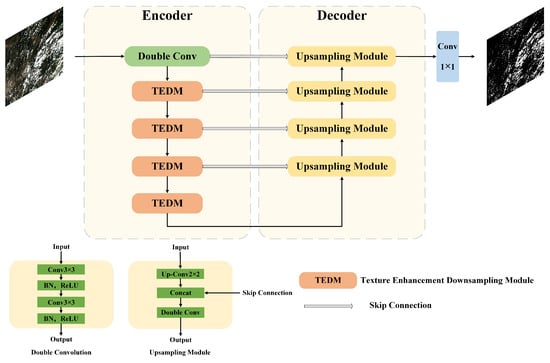
Figure 2.
The overall architecture of TENet. TENet first uses an encoder to extract features. The encoder incorporates the proposed TEDM to extract texture, channel, and spatial features. The decoder restores the spatial dimensions of the image through upsampling while reducing the number of feature channels. To facilitate multi-scale feature integration, skip connections are implemented to concatenate feature maps from corresponding encoder layers with their decoder counterparts at each stage of the decoding process.
The first layer of the encoder in the TENet is a double convolutional layer, which helps the network capture and learn richer feature representations during the downsampling process. This architecture comprises two sequential 3 × 3 convolutional layers, each followed by Batch Normalization (BN) and ReLU activation. The conventional downsampling module in U-Net is replaced by TEDM, which combines Haar wavelet transformation with the Convolutional Block Attention Module (CBAM) to facilitate more comprehensive learning of texture, channel and spatial features. The upsampling module employs a 2 × 2 transposed convolution followed by feature concatenation with corresponding-level feature maps from TEDM, subsequently processed through dual convolutional layers for feature refinement. Through the integration of skip connections and deconvolution-based feature fusion mechanisms, low-level encoder features are effectively combined with high-level decoder features to preserve detailed image information. The network generates final cloud predictions through a 1 × 1 convolutional layer, with probability values normalized to the [0, 1] range using a sigmoid activation function. Binary cloud detection results are obtained through threshold segmentation, where pixels with probability values exceeding threshold p are classified as cloud pixels. Threshold p serves as a critical hyperparameter that determines the classification boundary in the cloud detection task, governing the decision threshold for distinguishing cloud pixels from non-cloud pixels.
3.2. Object-Oriented Dynamic Threshold Pseudo-Cloud Pixel Labeling Method
Considering the variety of cloud types such as cirrus, cumulus, and stratus, which exhibit complex geometrical structures and uneven spectral reflectance, along with interference from complex land cover scenes (e.g., desert salt–alkali regions, snow-covered mountains, snowfields, and certain urban areas with high-brightness building rooftops), where the spectral characteristics of bright surfaces are highly similar to those of clouds [19], traditional cloud classification algorithms often assume a globally optimal segmentation threshold, which may lead to local errors.
To overcome this limitation, we developed a dynamic threshold cloud mask labeling approach that accounts for the spectral variability of cloud features. Conventional cloud detection algorithms are constrained by their reliance on static threshold values, which frequently lead to increased classification errors in specific regions. Additionally, these methods typically necessitate manual threshold adjustment for different geographical areas, prompting our focus on developing adaptive threshold calculation methodologies.
By initially observing a large amount of RS imagery containing clouds, we found that clouds always appear in the brighter regions of the image, while shadows are found in the darker parts. Based on the histogram of the grayscale image, we applied an improved triangular thresholding method to generate three dynamically adjustable thresholds, , , and , which represent the high-confidence cloud mask threshold, low-confidence cloud mask threshold, and shadow mask threshold, respectively.
Specifically, the algorithm flow of the triangular thresholding method can be described as follows: First, set the point (0,0) as one endpoint. Then, within the pixel brightness range of [125, 254] in the histogram, set the highest point of the most frequent brightness value as the other endpoint. Next, connect these two points with a line and calculate the distance between each brightness peak in the range [125, 254] and the drawn line. The point with the longest distance is multiplied by the pixel distance corresponding to each brightness level in the grayscale image to set the baseline threshold T. Finally, since this algorithm is fundamentally an image binarization method designed for processing positive samples during training, and based on extensive observations and empirical evidence, the gray value thresholds for thick clouds, thin clouds, and shadow regions exhibit a strong correlation with the generated thresholds T, , , and , which are set to 120%, 80%, and 30% of T, respectively. In empirical observations, clouds are often the areas with higher reflectivity in RS images. This algorithm ensures that the selected baseline threshold T will always be greater than 125, avoiding using the grayscale value of the surface with a large area and low reflectivity as the threshold T in scenes with few clouds.
After calculating these three key adaptive dynamic thresholds, we refer to Zhong’s method [13] and apply them to the improved ACCA algorithm to generate shadow masks, high-confidence cloud masks, and low-confidence cloud masks.
In the mask generation process represented in Figure 3, Band 1 (B1), Band 2 (B2), Band 3 (B3), and Band 4 (B4) represent the blue, green, red, and near-infrared bands, respectively. The ratio is utilized to differentiate vegetation from clouds, as well as shaded and non-shaded areas, while is employed to distinguish between soil and clouds. The values , , and are parameters referenced from the ACCA algorithm [11,13]. Clouds and cloud shadows exhibit an affine invariance relationship, where affine transformation, as a linear transformation, preserves the parallelism and collinearity of geometric features. Specifically, this transformation maintains properties such as parallelism preservation, single ratio invariance, and area ratio invariance. As clearly illustrated in Figure 4, during the matching process of the shadow mask and high-confidence cloud mask in the algorithmic workflow, the affine invariance relationship between clouds and cloud shadows is utilized to align the pixel counts of the two objects along the sun azimuth direction, as indicated by the green boxes in (a) and (c). This alignment enables the calculation of the center point deviation between the two boxes, which serves as the offset for a scene image, specifically represented by the red short line in (b). Since some high-brightness surfaces are included in the low-confidence mask, this offset can be employed to filter out incorrect labels, ultimately generating effective pseudo-labels suitable for deep learning training.
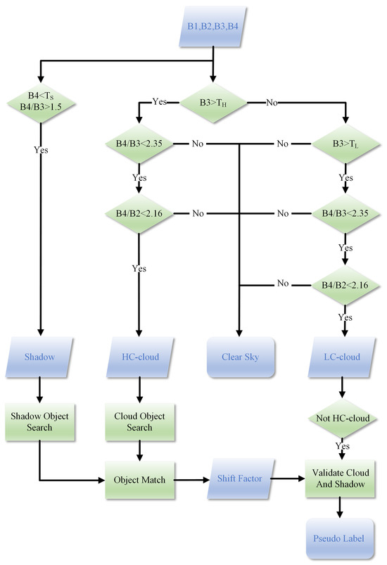
Figure 3.
The object-oriented cloud matching algorithm.
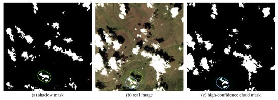
Figure 4.
Successful cases of object-oriented cloud matching algorithm.
Specifically, the process is executed in four sequential steps. First, cloud and shadow objects are identified within the generated high-confidence cloud mask and shadow mask, respectively. These objects are characterized by their center point coordinates, overall size, and the coordinates of their top, bottom, left, and right boundaries. Second, clearly separated cloud and shadow objects are searched within the image. By evaluating their relative spatial positions (top, bottom, left, right) and object sizes, successful matching is achieved when the objects fall within a strictly defined range. Third, as illustrated in the figure, the offset factor is calculated based on the center point coordinates of the matched cloud and shadow objects. Fourth, within the low-confidence cloud mask, the offset relationship is utilized to verify the correspondence between clouds and their shadows. This step effectively eliminates misclassifications caused by high-reflectivity surfaces, thereby generating accurate pseudo-labels for the clouds. If no successful match is identified, the final result defaults to the high-confidence cloud mask, ensuring the high accuracy of the training data.
3.3. Texture-Enhanced Downsampling Module
For challenging classification scenarios, such as distinguishing thin clouds and high-brightness surface environments, it is evident that easily classified thick clouds exhibit strong texture similarities with thin clouds in remote sensing images, while the textures of thick clouds and high-brightness surface environments are significantly distinct. Specifically, the brightness of thin cloud regions is lower than that of thick cloud regions, but their texture features are more pronounced. In contrast, the brightness of high-brightness surface areas is similar to that of thick cloud regions, but their textures are distinctly different. As illustrated in several cases in Figure 1, the texture of snow-covered mountains appears as fine dots along the mountain range shadows, while the texture of snow and saline–alkali land is subtle and resembles the central area of thick clouds; however, the edges of these regions differ from those of thick clouds, and the shadows of clouds are more distinct. This phenomenon is particularly evident in urban areas, where high-reflectivity surfaces on building tops are scattered and small in size. Consequently, leveraging texture feature learning emerges as a natural approach to enhance recognition accuracy. This necessitates the incorporation of an efficient texture feature learning method into the DL network. To address this issue, researchers have proposed methods such as the gray-level co-occurrence matrix and frequency domain processing techniques [33]. However, due to the fixed sampling positions in convolutional kernels, a significant amount of fine texture features can be lost. Inspired by HWD [14], this work demonstrates that features extracted using the HWD module help make texture information clearer. In practical applications, we analyze the characteristics of cloud regions under wavelet transformation. As illustrated in Figure 5, during the wavelet transform, the texture features of the cloud regions, represented by the vertical and horizontal high-frequency components in the lower left and upper right corners of the resulting image, become significantly more distinct. Additionally, all low-frequency background information is effectively filtered out, which facilitates the extraction of texture features from both vertical and horizontal directions. Observing the actual wavelet transform results inspired the design of the TEDM.
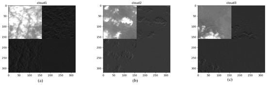
Figure 5.
Features extracted by first-level wavelet transform under different cloud amounts. (a–c) represent scenarios with high, moderate, and low cloud cover, respectively. In each image, the upper left and lower right corners correspond to low-frequency information and high-frequency information, while the lower left and upper right corners represent vertical and horizontal high-frequency components, respectively. The horizontal and vertical units represent the position of the image.
Rather than directly substituting the downsampling module of U-Net with HWD, we take into account the distinctive spectral inter-channel characteristics of clouds, snow-covered mountains, saline–alkali land, and other terrains, as well as the spatial connectivity of clouds. In the process of generating pseudo-cloud label datasets in our previous work, we incorporated the complex calculation of cloud channel characteristics, particularly the apparent reflectance data across different bands, as inspired by the traditional ACCA algorithm. During the object-oriented validation of the dataset, we observed the spatial continuity of clouds and their corresponding shadows. Consequently, when designing the downsampling module, it was natural to consider a learning module that enhances both channel and spatial features. In the downsampling module, as illustrated in Figure 6, we replace the original max pooling operation of U-Net with a wavelet transform downsampling module to better distinguish the texture features of clouds and non-cloud regions. Following two convolutional operations, a channel-space attention mechanism is applied to the resulting feature map.
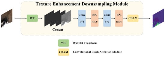
Figure 6.
The proposed TEDM process.
In our entire model, the proposed TEDM replaces the original downsampling module in U-Net, while the other model details remain unchanged. Specifically, the entire TEDM process can be described as follows:
First, the input feature map undergoes a first-level Haar wavelet transform, splitting it into four parts: the low-frequency approximation component (), the horizontal detail component (), the vertical detail component (), and the diagonal detail component ().
These four parts are then concatenated to form .
Next, undergoes two convolution operations for feature extraction. After each convolution, the resulting feature map is passed through a BN layer for normalization, reducing internal covariate shift and accelerating model convergence. Then, the normalized feature map undergoes a nonlinear transformation through the ReLU activation function to enhance the model’s expressive power. The two convolutions produce feature maps and .
For the subsequent CBAM attention mechanism, it can be split into two submodules: the channel attention mechanism (CAM) and the spatial attention mechanism (SAM). These two mechanisms enhance the features in the channel and spatial dimensions, respectively. Here, F represents the input feature map, and represent global average pooling and max pooling operations, respectively. represents a multi-layer perceptron, and is the sigmoid activation function used to output the channel attention weights. represents a convolution operation with a kernel size of .
Finally, the feature map generated by the channel attention mechanism, , is multiplied by the feature map from the previous step to generate . The feature map generated by the spatial attention mechanism, , is then multiplied by to generate the final output feature map .
3.4. Loss Function
This study defines the cloud detection task as a semantic segmentation problem, generating binary masks of clouds and background in the pixel classification task. Given the scarcity of samples in the dataset for regions such as snowy mountains, saline–alkali lands, and bright urban surfaces, Focal Loss is employed as the model’s loss function. The primary advantage of Focal Loss is its ability to reduce the impact of easily classified samples during training, allowing the model to focus more on hard-to-classify samples. This effectively addresses the issues of class imbalance between positive and negative samples and imbalance between easy and hard samples [34].
Focal Loss is an improvement on the cross-entropy loss function, and its formula is
In the above formula, y represents the pseudo-label of the cloud, which is a binary value indicating whether the sample belongs to the positive class. is the model’s predicted output, a continuous value between 0 and 1, representing the model’s confidence in predicting the pixel as a cloud. The focus parameter adjusts the model’s attention between hard-to-classify thin cloud regions and easy-to-classify thick cloud regions. By increasing the value of , the model reduces attention to the easily separable thick cloud regions, and focuses more on the hard-to-classify thin cloud regions, thus encouraging the model to improve classification accuracy for these samples. The class balance parameter addresses the issue of class imbalance in cloud data, by assigning different weights to different classes, thereby enhancing the model’s focus on minority classes. Especially in binary classification problems, an increase in results in greater penalization for misclassification of the minority class, which improves the model’s classification performance on minority categories. The range and optimal values of these two parameters should be adjusted based on the specific task and dataset, typically determined through methods such as cross-validation. Through the flexible adjustment of these two parameters, Focal Loss can effectively adapt to different data distributions and task requirements, improving the model’s performance in various scenarios.
4. Experiment and Analysis
This section evaluates the proposed framework on the GF-1 RS imagery dataset created by our team [35]. Specifically, we first introduce the motivation behind creating the dataset and the processing details, followed by a description of the experimental setup. Then, we present the ablation experiments on TENet. Finally, we provide both quantitative and qualitative analyses of the overall model performance.
4.1. Dataset
The initial goal of our work was to improve cloud detection accuracy in difficult-to-classify regions. Considering the large volume of the original data and the need to increase the proportion of difficult-to-classify surfaces in typical datasets, we ultimately decided to create a dataset with a higher proportion of challenging surfaces. We obtained 1107 Level-2 WFV scenes from the analysis-ready data (ARD) of the GF satellite data [35], covering various land types including forests, bare land, Gobi, deserts, snow-covered areas, snow-capped mountains, arable land, and urban regions. The GF-1 and GF-6 satellites are equipped solely with blue, green, red, and near-infrared bands, lacking thermal–infrared and shortwave–infrared bands. Each image has a size of pixels with four spectral bands. These selected images were produced after radiometric calibration and system correction.
After applying the object-oriented dynamic threshold cloud detection method, we observed that the accuracy in general grassland, forest, bare land, and ocean areas was very high, and thus, these images were considered suitable for training in the subsequent process. However, after reviewing the results in the more difficult regions, we found that the misdetection rate was relatively high, with many snow-capped mountains, snowfields, and deserts being mistakenly identified as clouds. Additionally, the detection rate in thin cloud regions was not very high.
After removing the images that caused difficulty in using the replacement strategy and had many missed detections, 475 images remained. In order to improve the credibility of the dataset, we employed two strategies to enhance the accuracy of labeling. The first strategy was to use low-confidence cloud masks generated by lenient thresholds instead of final masks with lower detection rates. The second strategy was to use a black mask instead of the final mask with a higher false detection rate. In Figure 7, the first row represents the first strategy, where (a) is the RS image and (b) is the final mask generated by the proposed object-oriented cloud matching algorithm. The low-confidence cloud mask in (c) clearly has higher detection rates, so it is used as the correct mask. The second row represents the second strategy, and similarly, (d) and (e) represent the RS image and final mask, respectively. There is significant false detection in (e), as the clouds in this scene are almost unobservable, so a cloud-free black mask is used as the correct mask. Specifically, 83 RS images used the two mentioned strategies, with 25 images using the first strategy and 58 images using the second strategy. This means that some challenging-to-classify positive and negative samples are added to the dataset.
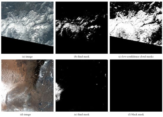
Figure 7.
Demonstration of two replacement strategies.
As shown in Table 1, the final dataset includes 475 scenes after partially using replacement strategies. The positive samples in our dataset are cloud pixels, and the negative samples are clear pixels. In our dataset, there are 173 challenging land cover scene images, including snow mountains, deserts, saline–alkali lands, and urban areas, accounting for 36.42% of the dataset. Because the false detection rate of the algorithm on the challenge image is high, the data of 58 images containing only negative samples are all from the replacement strategy. A total of 115 images contain positive and negative samples. The rest were 302 non-challenge images, including forest, grassland and crop areas. The mask generated by the algorithm has high accuracy in these areas, and only some use the replacement strategy. Among them, 28 images only contain negative samples, and 274 images contain positive and negative samples. In contrast, the WHU GF-1 WFV dataset [15], which consists of 108 complete images, contains challenging land cover scenes in 14 images, representing 12.96% of the total data volume. Our dataset has significantly increased in both the total volume and the proportion of challenging scenes, which facilitates the subsequent extraction of features under bright surface conditions and the completion of DL training. In accordance with standard practices, this experiment used an 8:8:3 ratio for training, validation, and testing. The division of the dataset is entirely random, without regard to the time of day when the images were acquired or their actual geographic locations. The original images were cropped into pixel tiles from left to right and top to bottom to accommodate limited computational resources.

Table 1.
The composition of positive and negative components of the GF-1 ARD dataset in challenge and non-challenge images.
During the testing phase, all cropped images were stitched back together to their original size for both quantitative and qualitative analyses and evaluation. It is worth noting that all the labels of our data were generated using the proposed object-oriented dynamic threshold pseudo-cloud pixel labeling method during the training phase, and the evaluation metrics were calculated based on the test set. Since the actual amount of ARD data from GF satellites is much larger than the scale of our dataset (475 images), and the pseudo-cloud labels generated in our WDCD framework are not entirely reliable, we also used some GF ARD data that were not included in the dataset for qualitative analysis. The actual locations were mainly selected in China, including desert saline–alkali lands in Northwest China, snow-capped mountains in Southwest China, forests and farmlands in Central China, grasslands and perennial snow-covered areas in North China, some marine areas, parts of Hainan Island where land and sea are connected, and some urban areas.
4.2. Evaluation Metrics
We use overall accuracy (), score, mean Intersection over Union (), and kappa coefficient () as quantitative metrics to evaluate the performance of TENet. All quantitative scores are calculated using the pixel-level references provided by the dataset. Note that, considering the labeling process, the accuracy of the dataset remains to be examined; however, after expert screening, the dataset roughly reflects the model’s performance. The definitions of these quantitative metrics are as follows:
In this context, , , , and represent the numbers of true positives, true negatives, false positives, and false negatives, respectively. The overall accuracy () is calculated as
where P and N are the numbers of cloud and clear sky pixels in the reference image, respectively. The expected accuracy () is calculated as
To evaluate the efficiency of the comparison methods, we assessed the number of model parameters and the number of floating-point operations (FLOPs) required to process a pixel image patch.
4.3. Implementation Details
When designing the network structure, we prioritized training efficiency, resource utilization, model simplicity, and robustness. After careful analysis, we selected a U-shaped network integrated with an attention mechanism, as it effectively combines detailed and semantic information while meeting the requirements for efficiency and stability in resource-constrained scenarios. In contrast, while DeepLabv3 and Transformer excel in large-scale data processing, their resource utilization efficiency is less optimal. Therefore, we ultimately chose U-Net as our baseline model. During the dataset creation process, we empirically set the three thresholds (, , and ) of the ACCA algorithm to 120%, 80%, and 30% of the threshold T, respectively, based on the triangular method. In the ACCA algorithm, the ratio of reflectance between , , and —specifically, and —is used to distinguish water bodies, vegetation, clouds, and cloud shadows. When , the threshold values and are used; if the ratios are below these values, the pixel is classified as cloud. When , the threshold for is applied; if the ratio exceeds this value, the pixel is classified as shadow.
During the object-oriented matching process, the number of object pixels is set within the range of [2000, 4000], the rectangle aspect ratio is within [0.95, 1.05], and the size ratio between cloud objects and shadow objects is within [0.85, 1.15]. Only when these conditions are met can the two objects be matched.
All DL experiments are implemented using the PyTorch 2.2.1 framework. The operating system used is CentOS 7, equipped with two NVIDIA Tesla P100 12G GPUs. TENet was trained for 80 epochs, with a batch size set to 8 and the learning rate set to . For comparison with classic experimental methods and ablation experiments, the same settings are applied where possible. For some methods, the batch size is set to 4 due to the network parameters and structure. In our dataset, it can be considered that the positive and negative samples are relatively balanced, based on the parameter setting experience of Focal Loss [34]; the Focal Loss parameters were set as and . During the testing phase, only one GPU was used.
4.4. Ablation Experiments
To evaluate the performance of TENet, we conducted ablation experiments on the TEDM, the CAM, and the SAM.
In this experiment, to minimize interference from extraneous factors, we used the U-Net model as the baseline and conducted the ablation on the downsampling module of the encoder. We kept other parts of the structure unchanged, with the experimental variables set to different downsampling methods, including max pooling and wavelet transformation. Another variable was the type of attention mechanism added, including the CAM and the SAM. As shown in Table 2, adding the CAM to the downsampling module resulted in a significant improvement in the accuracy of the baseline model. When combined with the SAM, the improvement from a data perspective was limited. However, from the practical prediction results, as shown in the figures, the model with CBAM exhibited lower misclassification rates on challenging surfaces and higher detection rates in thin cloud areas. Our model achieved the best performance both in terms of data and practical results.
Table 2.
Effectiveness of TEDM components on the GF-1 ARD dataset.
As shown in Figure 8d, without adding any attention mechanism, the large desert area above is recognized as a cloud. In this scenario, both CAM+U-Net and CBAM+U-Net performed well; the results of both are similar to those shown in Figure 8c. It is clearly visible that in the case of high-brightness surfaces, our model significantly reduces the misdetection rate. These results support the idea that after adding the channel attention mechanism to the model, large-scale misdetections can be reduced. With deeper feature learning along the channel dimension, the model’s accuracy is significantly improved.
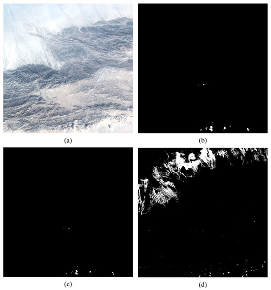
Figure 8.
Comparison of TENet and baseline results. (a) is the original image, (b) is the ground truth, (c) is the prediction result of TENet, and (d) is the prediction result of U-Net.
In some details, such as the sunlit slopes of the mountains in the above image, the spectral characteristics of the high-brightness surface under sunlight are very similar to those of clouds. As shown in the red circles in Figure 9c,d, there are many small misdetections. However, TENet, which focuses more on texture features, as shown in Figure 9b, is able to exclude some of these small misdetections.
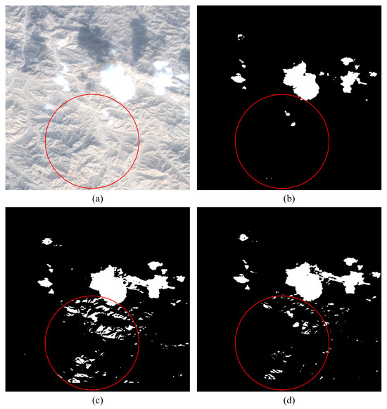
Figure 9.
Comparison of CAM, SAM, and wavelet downsampling. (a) is the original image, (b) is the prediction result of TENet, (c) is the prediction result of CBAM+U-Net, and (d) is the prediction result of CAM+U-Net.
4.5. Comparison
We evaluated our proposed model against several other methods using the GF-1 ARD satellite image dataset. As presented in Table 3, TENet demonstrates superior performance across the four selected metrics compared to the other methods. The models used in this experiment are established classics in the field of DL. Owing to its emphasis on robust texture detail extraction, TENet excels in accuracy, particularly on challenging surfaces such as snow-covered mountains, snowy regions, desert salinized land, and urban high-reflectivity areas, where it holds a significant advantage. Notably, while FCN exhibits commendable accuracy in cloud detection tasks, it still incurs higher misdetection rates on difficult-to-classify surfaces compared to our model. Furthermore, the parameter count of the FCN model is orders of magnitude greater than that of our proposed model. In practical applications, both the training time and prediction time per image for FCN are also substantially higher than those of the other models under comparison.
Table 3.
Comparative experiment on GF-1 ARD dataset.
As shown in Figure 10, in the forest area, the prediction results from all four models are quite clear, but FCN, due to its characteristics, produces results with more blurred boundaries. This scene is one of the easiest to classify in practice because the difference between the surface and the clouds is particularly significant. In our dataset, which was designed with easy-to-classify surfaces, the results are generally good.
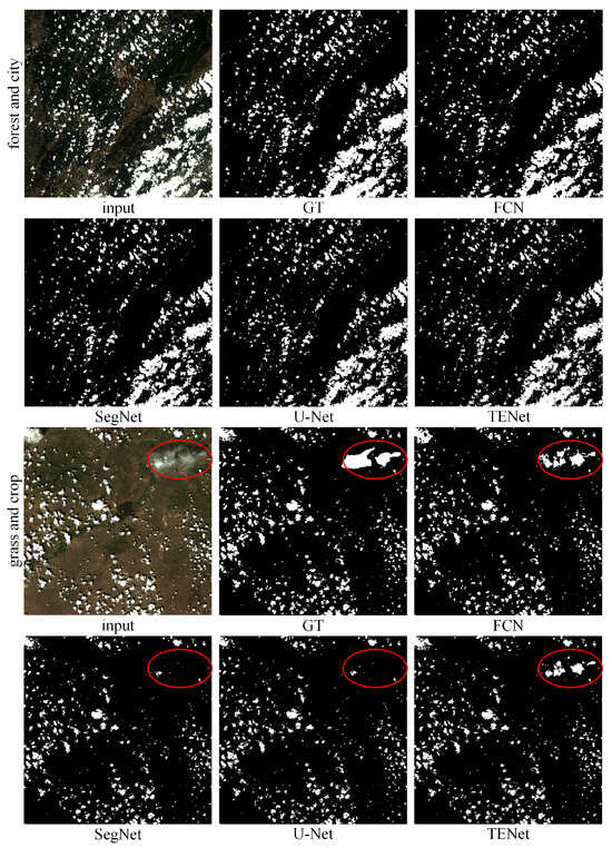
Figure 10.
Comparison of results in forest and grassland scenarios.
In the grassland and cropland prediction results, overall, all four models show very high prediction accuracy. However, there is a noticeable difference in performance in the thin cloud areas, which are marked by red circles. FCN, due to its parameter settings and learning depth, performs the best. SegNet and U-Net seem to learn less from the features of thin cloud areas. Our proposed model, TENet, focuses more on texture, channel, and spatial features, and performs slightly better than SegNet and U-Net in detecting thin cloud regions.
As shown in Figure 11, in the saline–alkaline land prediction results, the differences between the four models are more pronounced. In the top-left portion of the image, FCN shows large misclassification errors, incorrectly detecting high-brightness desert regions as thin cloud areas. In the bottom-right portion of the image, in the high-brightness saline–alkaline area, the first three models all show some degree of misclassification. Overall, our results are very successful, though a small error in prediction appears in the bottom-right portion.
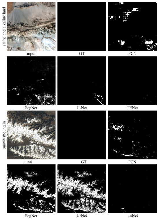
Figure 11.
Comparison of results in saline–alkaline land and snowy mountain scenarios.
In the snowy mountain region, FCN’s misdetections are mainly concentrated in the high-brightness mountain peak areas, where parts of the continuous high-brightness snow areas are incorrectly detected as thick cloud regions. SegNet and U-Net show even larger misclassification areas in this region. Our model’s error rate is very low.
4.6. Challenging Image Analysis
The most challenging task in cloud detection is identifying cloud layers in challenging surface scenes. These scenes include the snowy mountains, snowy terrain, desert saline, alkali land, and urban areas. We used 1000 surface scenes not included in the dataset for the qualitative analysis of the prediction results, which consisted of 700 challenge images and 300 non-challenge images. During the experiment, we adjusted the hyperparameters of TENet based on quantitative analysis of the dataset and qualitative analysis of additional challenging images to achieve optimal performance. The results of partial desert saline and alkaline land are shown in Figure 8c and Figure 9b. It can be clearly observed that clouds can be detected in these scenes, and the highlighted surfaces were not detected incorrectly.
In Figure 12, the first three rows show the comparison of the prediction results of the model in the scene with snow. In the first row, clouds can be clearly identified in the image. In the prediction results of TENet, the snow mountain in the lower right corner was not detected as cloud, while the thick cloud in the middle of the image was detected. In the results of SegNet and U-Net, the snow mountain in the lower right corner generally has false detection. In the upper left corner of the mixed cloud shadow and snow part, the FCN, SegNet and U-Net results have a small amount of false detection. In the second row, the clouds and snow in the middle of the image are mixed, which is difficult to classify. The cloud on the right side of the image can be detected by four methods. In the prediction results of TENet and FCN, the position marked by the red circle lacks the detection of thin clouds on the snow. In the results of SegNet and U-Net, there are many false detections in the position of the red rectangle mark. In the third row, it is obvious that the snow mountain in the upper right corner of the image is very clear and not covered by clouds. Clouds are mainly concentrated on the snow mountain in the middle and lower right corner. In the prediction results of TENet and FCN, clouds and snow mountains can also be distinguished. However, in the blue circle of the image, due to the block prediction, it can be clearly observed that there are still a small number of missing clouds in TENet. In the results of FCN, SegNet and U-Net, part of the snow mountains in the upper left corner and lower left corner were mistakenly detected as clouds. In the fourth row, the cloud layer and the highlighted reflective artificial surface of the city can be clearly distinguished. Compared with the scene in Figure 1d, it is obvious that DL methods significantly reduce the false detection rate of urban areas.
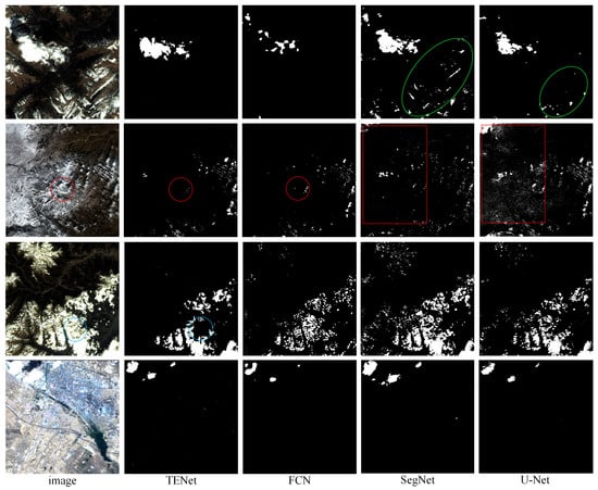
Figure 12.
Comparison of prediction results on challenging images.
5. Conclusions and Discussion
In methods for cloud detection with the GF-1 and GF-6 datasets, the accuracy on challenging surfaces—such as snow-covered mountains, saline–alkali lands within deserts or Gobi, the snow-covered surfaces—remains relatively low, and the efficiency for collecting samples to train the prevalent DL-based methods relies heavily on large amounts of pixel-level annotations, which are both time-consuming and labor-intensive. Subsequently, we propose a WDCD framework that integrates an object-oriented dynamic threshold labeling method and a DL network with TEDM to enhance both the efficiency of the DL method and the detection accuracy over challenging surfaces. On the one hand, an overall accuracy of 96.98% was achieved on the GF-1 ARD dataset. On the other hand, through the qualitative analysis of the prediction results of 1000 ARD images not in the dataset, it can be concluded that the model can reduce the false detection rate of the challenging high-brightness surface, so as to improve the quality of cloud detection.
For the first time, an object-oriented dynamic threshold labeling method leveraging object-oriented principles and dynamic thresholding techniques was developed, and a large amount of samples of challenging surfaces were effectively and efficiently collected. More precisely, this method calculates dynamic thresholds for the image and removes unreasonable results by leveraging the affine invariance relationship between clouds and cloud shadows along with an object-oriented approach, generating a training set with a large amount of samples, which provides a executable solution to quickly and effectively retrieve the training samples for the DL method. More importantly, this labeling method can effectively collect samples for challenging surfaces, such as snow-covered mountains and saline–alkali lands.
Subsequently, by considering the spatial continuity of clouds, the correlation across channels, and their distinctive texture features, a texture-feature-enhanced attention module is designed to strengthen the learning of difficult positive and negative samples on challenging surfaces. These pseudo-masks are then applied to the proposed cloud detection DL framework. Experiments show that the comprehensive attention module can better capture the features of those challenging surfaces and subsequently improve the identification accuracy. The visual comparisons show the extraordinary performance on challenging surfaces.
In summary, our model demonstrates exceptional performance on high-brightness surfaces. This can be attributed to two key factors. First, our model is backed by a dataset that comprises high-quality negative samples. These samples provide a diverse and representative range of data, enabling the model to better understand and distinguish different features. Second, our model incorporates attention mechanisms for texture, spectral, and spatial aspects. The texture attention mechanism allows the model to focus on surface details, capturing subtle variations that may be indicative of specific properties. The spectral attention mechanism enables the model to analyze and utilize information across different wavelength bands, which is crucial for accurately interpreting the interaction of light with surfaces. The spatial attention mechanism helps the model to consider the spatial relationships between different regions of the surface, providing a more comprehensive understanding of the surface structure. Together, these factors significantly enhance the model’s ability to handle high-brightness surfaces effectively.
When evaluating the generalization of our method to Sentinel-2, Landsat-8, and MODIS, it is important to note that, since our dataset lacks thermal–infrared and shortwave–infrared bands, our approach primarily focuses on distinguishing between cloud and non-cloud pixels at the image level. If the data includes thermal–infrared bands, it would enable better differentiation between clouds, deserts, saline–alkali lands, and ice-covered surfaces based on temperature. Similarly, if the data includes shortwave-infrared bands, it would facilitate improved distinction between clouds and water bodies or vegetation. These band data can enhance accuracy and improve the distinction of challenging surfaces during the automated construction of WDCD datasets. In designing the attention mechanism for the DL network, these band data can also be more effectively utilized with the CAM, offering additional opportunities to innovate new attention mechanisms, such as incorporating color and temperature attention mechanisms.
When considering the limitations of our approach, several points warrant attention, many of which are tied to our semi-automatic dataset construction process, as our ultimate goal is to achieve full automation in generating usable, high-quality datasets. First of all, although the dataset has achieved more efficient annotation efficiency, it still requires a small amount of manual review work. Secondly, the network can be optimized to further shorten the prediction time for each scene image. Thirdly, the network can be used for other RS images with little modification, and the evaluations for the other RS images can be carried out in the near future to extend the applicability of the proposed network. In addition, the samples for thin clouds are still few and the features of thin clouds are very similar to the situations with thick aerosols, so the identification accuracy remains the lowest. Thus, how to solve this issue is our next and primary mission.
In the domain of cloud detection, future research directions emphasize the integration and innovation of multi-technology approaches to enhance detection accuracy and operational efficiency. This encompasses advancements in spatiotemporal fusion, super-resolution techniques, and transfer learning methodologies. Spatiotemporal fusion technology is anticipated to augment the monitoring capabilities of dynamic cloud variations by synthesizing data with diverse temporal and spatial resolutions. A promising avenue for future research lies in enriching feature diversity through the fusion of spatiotemporal features and the aggregation of guidelines, facilitating improved differentiation between clouds and challenging surfaces based on temporal characteristics. Super-resolution fusion technology is expected to elevate the spatial resolution of imagery by integrating hyperspectral and multispectral datasets, thereby enabling more precise identification of cloud attributes. This perspective motivates further exploration into the potential of data reconstruction within the WDCD process to achieve superior texture feature learning outcomes.
We anticipate that the ongoing advancements in artificial intelligence and big data technologies will drive future research toward a more integrated approach, combining data-driven and model-driven methodologies. Deep learning techniques are expected to play a pivotal role in extracting valuable insights from multi-source datasets, while the incorporation of physical models will significantly improve the interpretability and robustness of cloud detection frameworks. This synergistic approach will enable the development of more reliable and comprehensive cloud detection systems.
Author Contributions
X.T. proposed the concept, conducted the experiments, and drafted the initial manuscript. B.Z. suggested improvements, analyzed the experimental results, and revised the initial draft. S.W. and K.A. proposed ideas for algorithm enhancements. X.L. reviewed and revised the manuscript. All authors have read and agreed to the published version of the manuscript.
Funding
This research was supported by the Hainan Provincial Natural Science Foundation of China (422QN350), the Science and Technology Fundamental Resources Investigation Program of China (2022FY100200), and the Beijing Science and Technology Plan (Z241100005424006).
Data Availability Statement
The data that support the findings of this study are available from the corresponding author on reasonable request.
Conflicts of Interest
The authors declare no conflicts of interest.
References
- Li, J.; Pei, Y.; Zhao, S.; Xiao, R.; Sang, X.; Zhang, C. A review of remote sensing for environmental monitoring in China. Remote Sens. 2020, 12, 1130. [Google Scholar] [CrossRef]
- Wang, X. Remote sensing applications to climate change. Remote Sens. 2023, 15, 747. [Google Scholar] [CrossRef]
- Weiss, M.; Jacob, F.; Duveiller, G. Remote sensing for agricultural applications: A meta-review. Remote Sens. Environ. 2020, 236, 111402. [Google Scholar]
- Wellmann, T.; Lausch, A.; Andersson, E.; Knapp, S.; Cortinovis, C.; Jache, J.; Scheuer, S.; Kremer, P.; Mascarenhas, A.; Kraemer, R.; et al. Remote sensing in urban planning: Contributions towards ecologically sound policies? Landsc. Urban Plan. 2020, 204, 103921. [Google Scholar]
- Simpson, J.J.; Stitt, J.R. A procedure for the detection and removal of cloud shadow from AVHRR data over land. IEEE Trans. Geosci. Remote Sens. 1998, 36, 880–897. [Google Scholar] [CrossRef]
- Chen, Y.; Tao, F. Potential of remote sensing data-crop model assimilation and seasonal weather forecasts for early-season crop yield forecasting over a large area. Field Crop. Res. 2022, 276, 108398. [Google Scholar]
- Gawlikowski, J.; Ebel, P.; Schmitt, M.; Zhu, X.X. Explaining the effects of clouds on remote sensing scene classification. IEEE J. Sel. Top. Appl. Earth Obs. Remote Sens. 2022, 15, 9976–9986. [Google Scholar]
- Mahajan, S.; Fataniya, B. Cloud detection methodologies: Variants and development—A review. Complex Intell. Syst. 2020, 6, 251–261. [Google Scholar]
- Liu, J.; Wang, X.; Guo, M.; Feng, R.; Wang, Y. Shadow Detection in Remote Sensing Images Based on Spectral Radiance Separability Enhancement. IEEE Trans. Pattern Anal. Mach. Intell. 2023, 46, 3438–3449. [Google Scholar]
- Wang, Z.; Zhao, L.; Meng, J.; Han, Y.; Li, X.; Jiang, R.; Chen, J.; Li, H. Deep learning-based cloud detection for optical remote sensing images: A Survey. Remote Sen. 2024, 16, 4583. [Google Scholar]
- Irish, R.R.; Barker, J.L.; Goward, S.N.; Arvidson, T. Characterization of the Landsat-7 ETM+ automated cloud-cover assessment (ACCA) algorithm. Photogramm. Eng. Remote Sens. 2006, 72, 1179–1188. [Google Scholar]
- Zhu, Z.; Wang, S.; Woodcock, C. Improvement and expansion of the Fmask algorithm: Cloud, cloud shadow, and snow detection for Landsats 4–7, 8, and Sentinel 2 images. Remote. Sens. Environ. 2015, 159, 269–277. [Google Scholar]
- Zhong, B.; Chen, W.; Wu, S.; Hu, L.; Luo, X.; Liu, Q. A cloud detection method based on relationship between objects of cloud and cloud-shadow for Chinese moderate to high resolution satellite imagery. IEEE J. Sel. Top. Appl. Earth Obs. Remote Sens. 2017, 10, 4898–4908. [Google Scholar]
- Xu, G.; Liao, W.; Zhang, X.; Li, C.; He, X.; Wu, X. Haar wavelet downsampling: A simple but effective downsampling module for semantic segmentation. Pattern Recognit. 2023, 143, 109819. [Google Scholar]
- Li, Z.; Shen, H.; Li, H.; Xia, G.; Gamba, P.; Zhang, L. Multi-feature combined cloud and cloud shadow detection in GaoFen-1 wide field of view imagery. Remote Sens. Environ. 2017, 191, 342–358. [Google Scholar]
- Tian, M.; Chen, H.; Liu, G. Cloud detection and classification for S-NPP FSR CRIS data using supervised machine learning. In Proceedings of the IGARSS 2019-2019 IEEE International Geoscience and Remote Sensing Symposium, Yokohama, Japan, 28 July–2 August 2019; IEEE: New York, NY, USA, 2019; pp. 9827–9830. [Google Scholar]
- Li, J.; Wu, Z.; Hu, Z.; Jian, C.; Luo, S.; Mou, L.; Zhu, X.X.; Molinier, M. A lightweight deep learning-based cloud detection method for Sentinel-2A imagery fusing multiscale spectral and spatial features. IEEE Trans. Geosci. Remote Sens. 2021, 60, 1–19. [Google Scholar]
- Zhang, J.; Wu, J.; Wang, H.; Wang, Y.; Li, Y. Cloud detection method using CNN based on cascaded feature attention and channel attention. IEEE Trans. Geosci. Remote Sens. 2021, 60, 1–17. [Google Scholar]
- Wu, X.; Shi, Z.; Zou, Z. A geographic information-driven method and a new large scale dataset for remote sensing cloud/snow detection. ISPRS J. Photogramm. Remote Sens. 2021, 174, 87–104. [Google Scholar]
- Chen, Y.; Weng, Q.; Tang, L.; Liu, Q.; Fan, R. An automatic cloud detection neural network for high-resolution remote sensing imagery with cloud–snow coexistence. IEEE Geosci. Remote Sens. Lett. 2021, 19, 1–5. [Google Scholar]
- Li, X.; Yang, X.; Li, X.; Lu, S.; Ye, Y.; Ban, Y. GCDB-UNet: A novel robust cloud detection approach for remote sensing images. Knowl.-Based Syst. 2022, 238, 107890. [Google Scholar]
- Zhu, X.; Helmer, E.H. An automatic method for screening clouds and cloud shadows in optical satellite image time series in cloudy regions. Remote Sens. Environ. 2018, 214, 135–153. [Google Scholar] [CrossRef]
- Buttar, P.K.; Sachan, M.K. Semantic segmentation of clouds in satellite images based on U-Net++ architecture and attention mechanism. Expert Syst. Appl. 2022, 209, 118380. [Google Scholar] [CrossRef]
- Chan, L.; Hosseini, M.S.; Plataniotis, K.N. A comprehensive analysis of weakly-supervised semantic segmentation in different image domains. Int. J. Comput. Vis. 2021, 129, 361–384. [Google Scholar] [CrossRef]
- Wang, S.; Chen, W.; Xie, S.M.; Azzari, G.; Lobell, D.B. Weakly supervised deep learning for segmentation of remote sensing imagery. Remote Sens. 2020, 12, 207. [Google Scholar] [CrossRef]
- Zhou, Y.; Wang, H.; Yang, R.; Yao, G.; Xu, Q.; Zhang, X. A novel weakly supervised remote sensing landslide semantic segmentation method: Combining CAM and cycleGAN algorithms. Remote Sens. 2022, 14, 3650. [Google Scholar] [CrossRef]
- Liu, Y.; Li, Q.; Li, X.; He, S.; Liang, F.; Yao, Z.; Jiang, J.; Wang, W. Leveraging physical rules for weakly supervised cloud detection in remote sensing images. IEEE Trans. Geosci. Remote. Sens. 2023, 61, 1–18. [Google Scholar] [CrossRef]
- Ma, H.; Liu, D.; Xiong, R.; Wu, F. iWave: CNN-based wavelet-like transform for image compression. IEEE Trans. Multimed. 2019, 22, 1667–1679. [Google Scholar] [CrossRef]
- Hu, J.; Shen, L.; Sun, G. Squeeze-and-excitation networks. In Proceedings of the IEEE Conference on Computer Vision and Pattern Recognition, Salt Lake City, UT, USA, 18–23 June 2018; pp. 7132–7141. [Google Scholar]
- Hu, J.; Shen, L.; Albanie, S.; Sun, G.; Vedaldi, A. Gather-excite: Exploiting feature context in convolutional neural networks. arXiv 2018, arXiv:1810.12348. [Google Scholar]
- Wang, F.; Jiang, M.; Qian, C.; Yang, S.; Li, C.; Zhang, H.; Wang, X.; Tang, X. Residual attention network for image classification. In Proceedings of the IEEE Conference on Computer Vision and Pattern Recognition, Honolulu, HI, USA, 21–26 July 2017; pp. 3156–3164. [Google Scholar]
- Woo, S.; Park, J.; Lee, J.Y.; Kweon, I.S. Cbam: Convolutional block attention module. In Proceedings of the European Conference on Computer Vision (ECCV), Munich, Germany, 8–14 September 2018; pp. 3–19. [Google Scholar]
- Baaziz, N.; Abahmane, O.; Missaoui, R. Texture feature extraction in the spatial-frequency domain for content-based image retrieval. arXiv 2010, arXiv:1012.5208. [Google Scholar]
- Ross, T.Y.; Dollár, G. Focal loss for dense object detection. In Proceedings of the IEEE Conference on Computer Vision and Pattern Recognition, Honolulu, HI, USA, 21–26 July 2017; pp. 2980–2988. [Google Scholar]
- Zhong, B.; Yang, A.; Liu, Q.; Wu, S.; Shan, X.; Mu, X.; Hu, L.; Wu, J. Analysis ready data of the Chinese GaoFen satellite data. Remote Sens. 2021, 13, 1709. [Google Scholar] [CrossRef]
Disclaimer/Publisher’s Note: The statements, opinions and data contained in all publications are solely those of the individual author(s) and contributor(s) and not of MDPI and/or the editor(s). MDPI and/or the editor(s) disclaim responsibility for any injury to people or property resulting from any ideas, methods, instructions or products referred to in the content. |
© 2025 by the authors. Licensee MDPI, Basel, Switzerland. This article is an open access article distributed under the terms and conditions of the Creative Commons Attribution (CC BY) license (https://creativecommons.org/licenses/by/4.0/).