
Pressure-Related Discrepancies in Landsat 8 Level 2 Collection 2 Surface Reflectance Products and Their Correction


Abstract
1. Introduction
1.1. Background
1.2. Issues in Surface Reflectance Products
1.3. Challenges
1.4. Research Objective
2. Materials
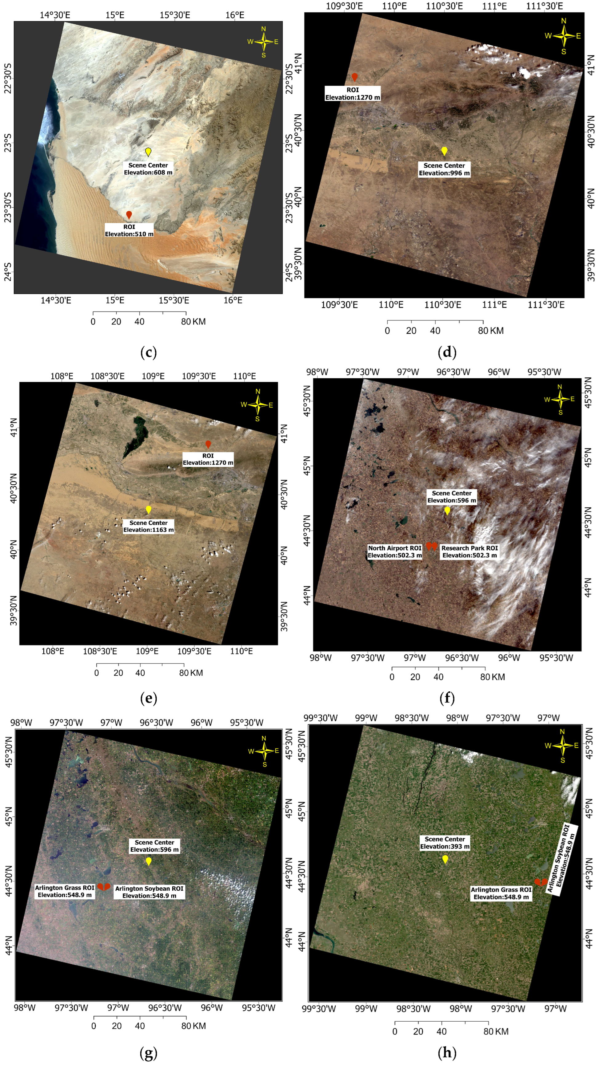
2.1. Study Areas
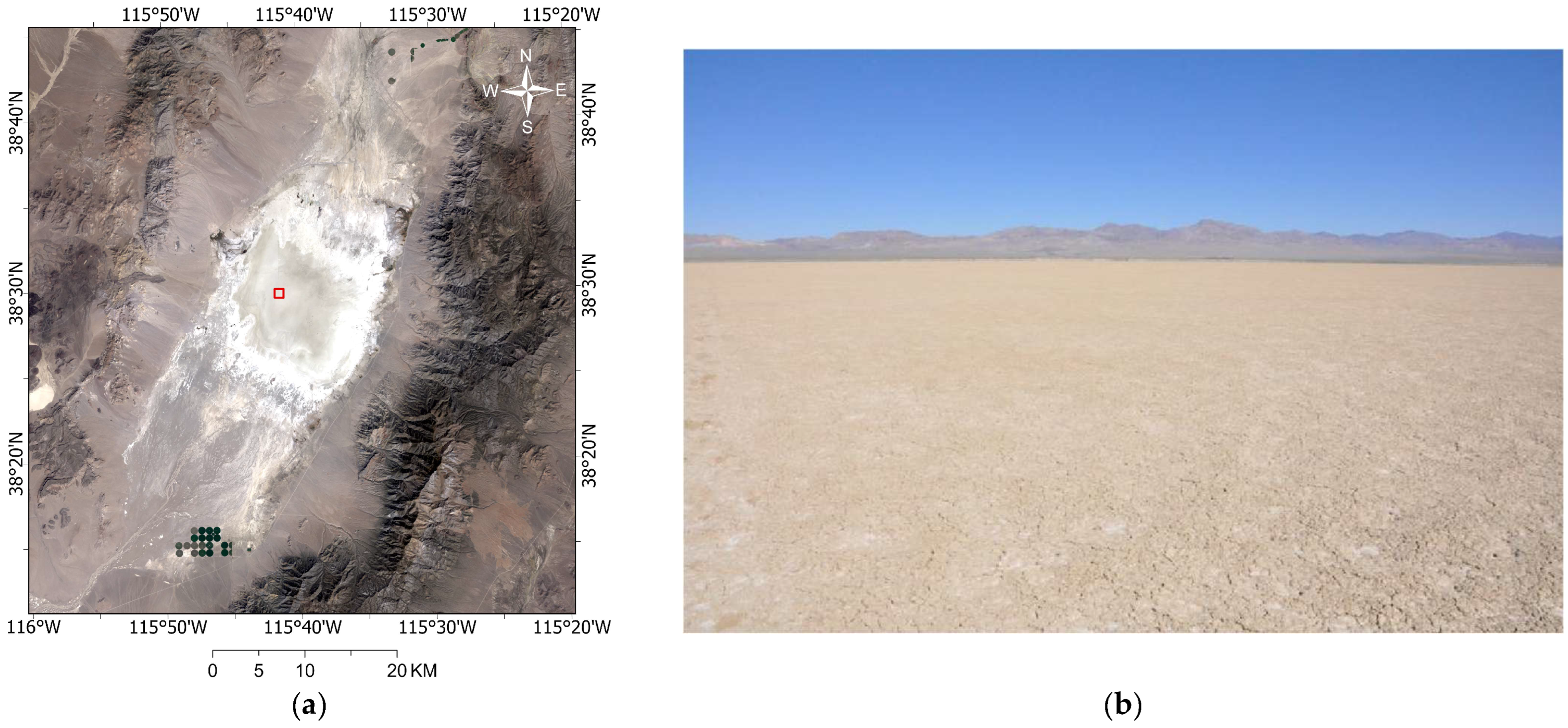
2.1.1. RadCalNet Site—Railroad Valley Playa
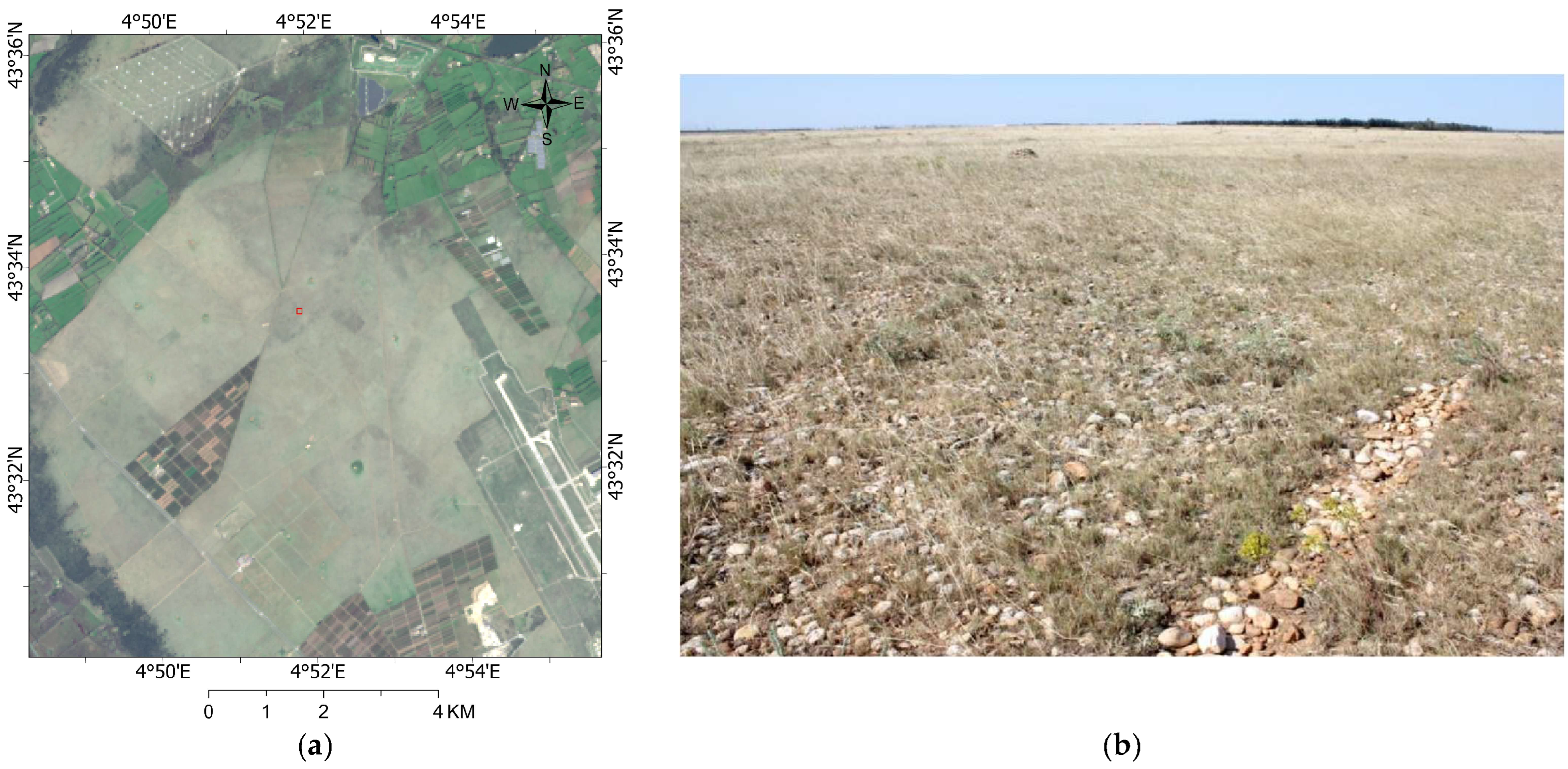
2.1.2. RadCalNet Site—La Crau
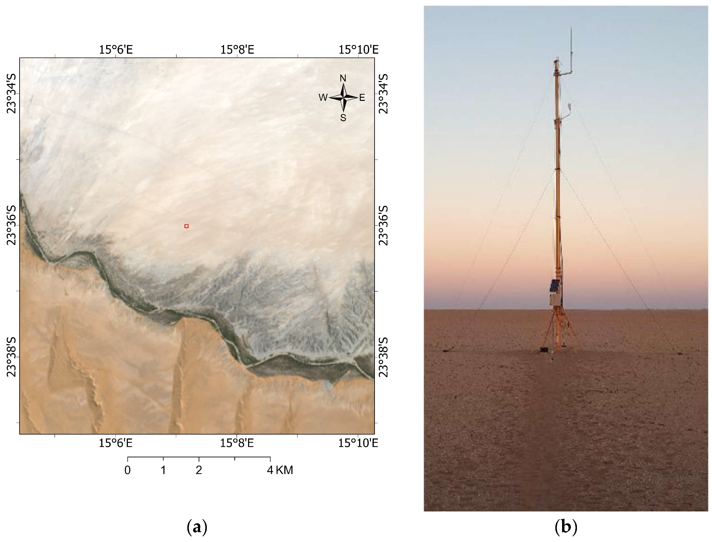
2.1.3. RadCalNet Site—Gobabeb
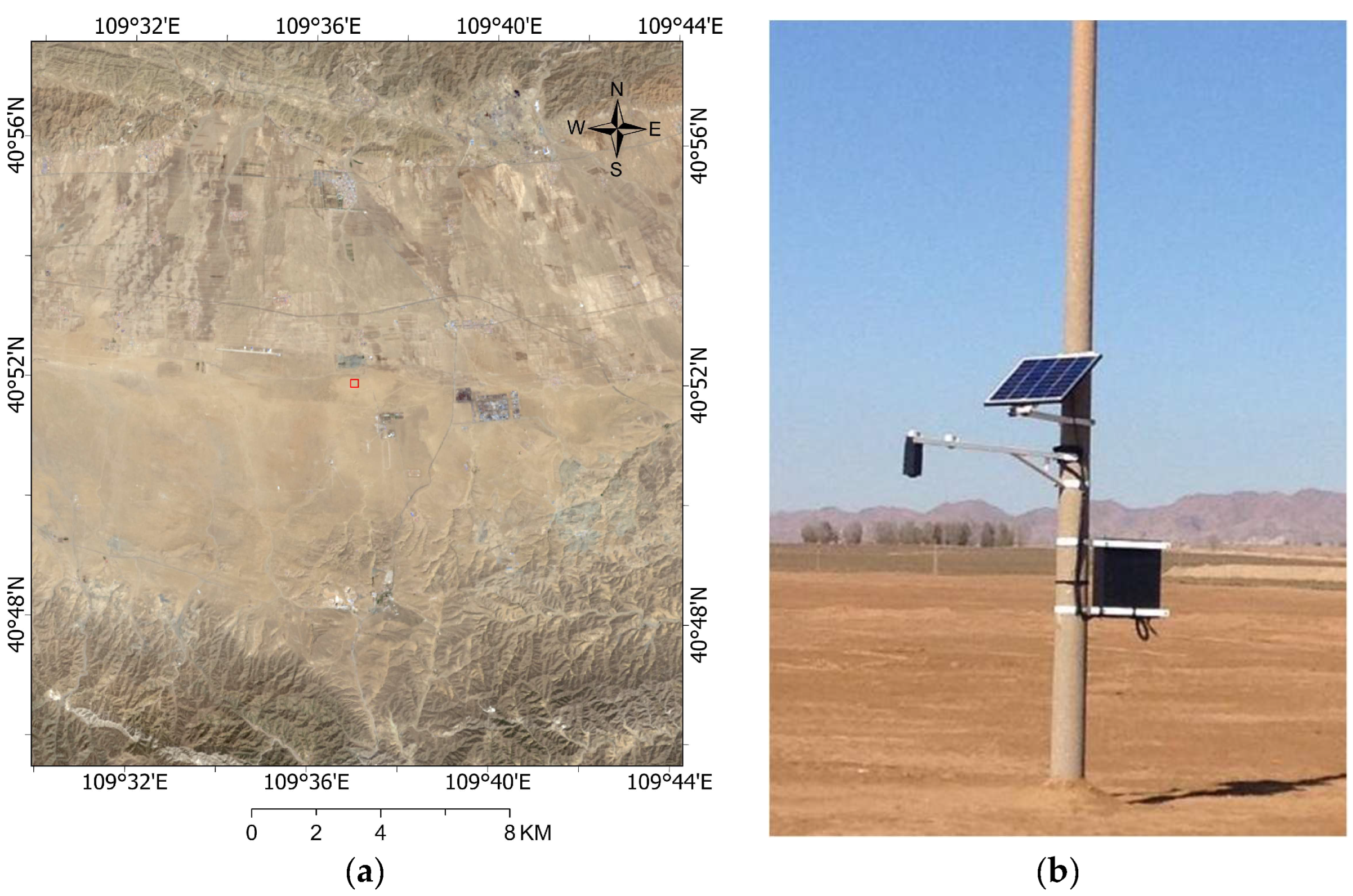
2.1.4. RadCalNet Site—Baotao Sand
2.1.5. South Dakota State University—SDSU Sites
2.2. Atmospheric Parameters
2.2.1. Aerosols
2.2.2. Absorbing Gases
2.2.3. Rayleigh Scattering
2.2.4. Surface Pressure
2.3. Landsat 8
2.4. Arable Mark 2 Sensor
3. Methodology
3.1. Land Surface Reflectance Code
3.1.1. Surface Reflectance Inversion in LaSRC
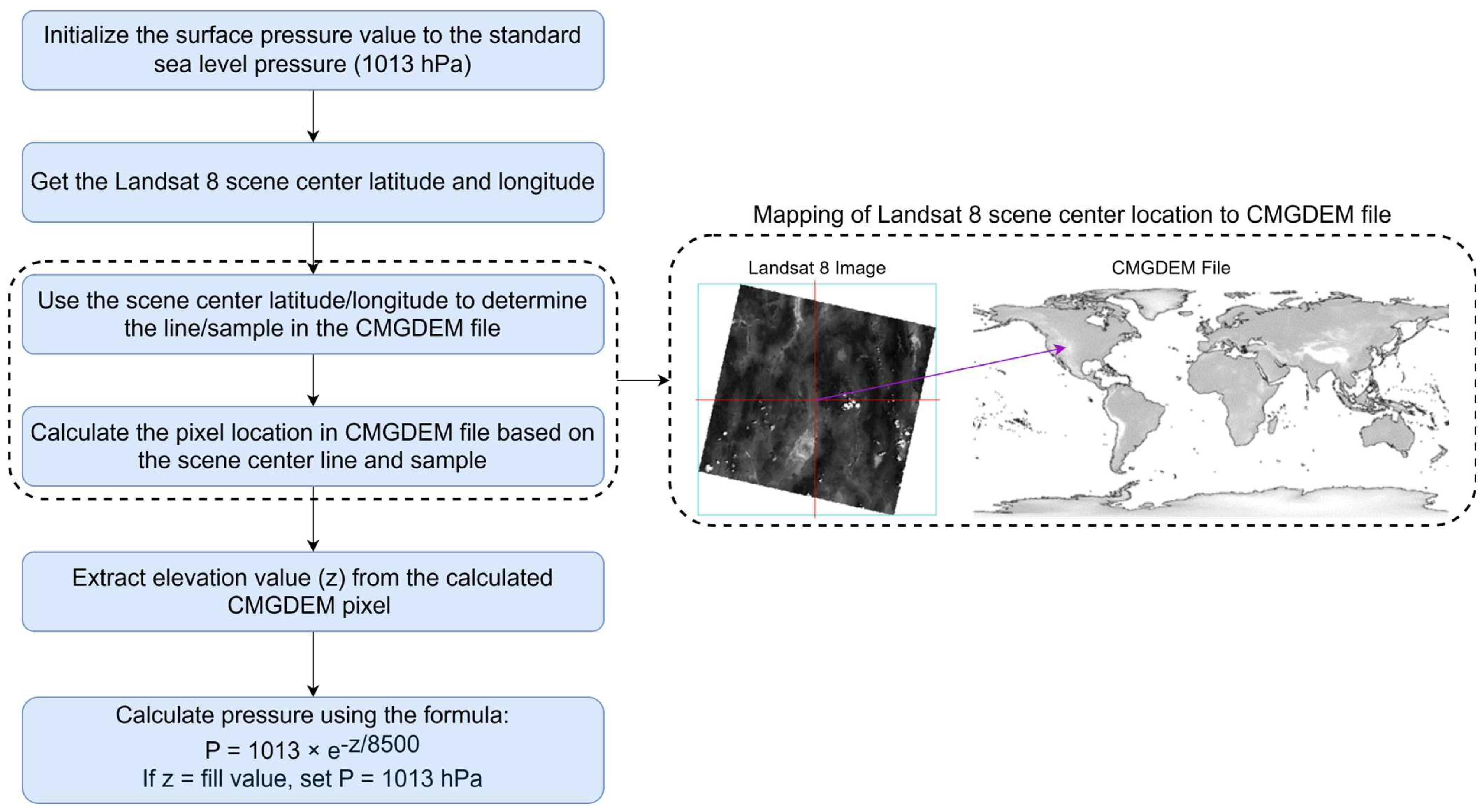
3.1.2. Calculation of LaSRC Surface Pressure for Landsat 8 Scene
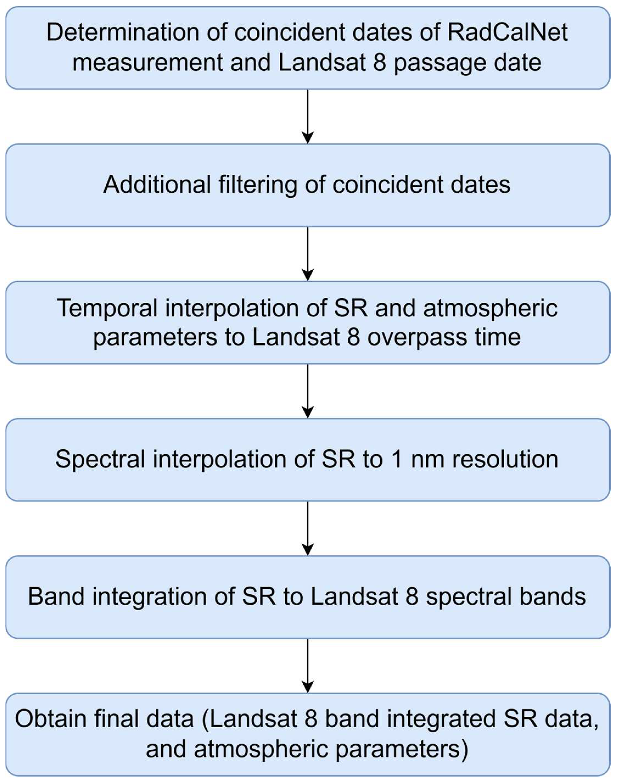
3.2. Data Processing for RadCalNet Sites
- There must be at least one RadCalNet measurement within one hour before the satellite overpass.
- There must be at least one RadCalNet measurement within one hour after the satellite overpass.
- A minimum of four RadCalNet measurements out of 13 available measurements throughout the day (from 17:00 to 23:00 UTC) must be present.
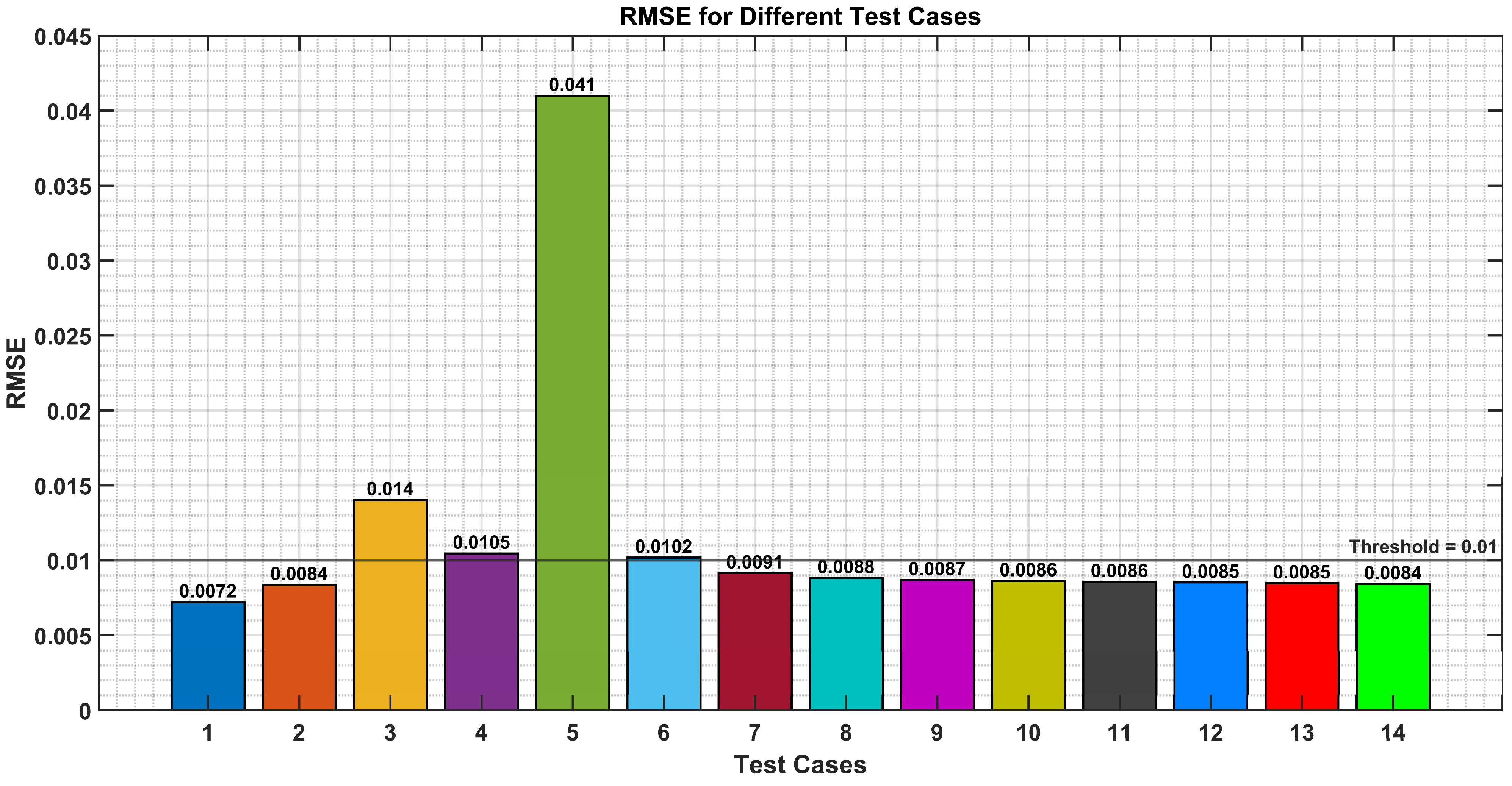
- Test case 1—All 13 RadCalNet measurements were included.
- Test case 2—The RadCalNet measurement at 18:30 was removed.
- Test case 3—Criterion 1 was removed (RadCalNet measurements at 17:30 and 18:00 were excluded).
- Test case 4—Criterion 2 was removed (RadCalNet measurements at 19:00 and 19:30 were excluded).
- Test case 5—Both Criteria 1 and 2 were removed (RadCalNet measurements from 17:30 to 19:00 were excluded).
- Test case 6—Criteria 1 and 2 were retained, but Criterion 3 was removed, leaving only three RadCalNet measurements.
- Test cases 7 to 14—Criteria 1, 2, and 3 were retained, and the number of RadCalNet measurements varied between 4 and 11, incrementing by one RadCalNet measurement for each test case.
3.3. Data Processing for Arable Mark 2 Sites
3.4. Landsat 8 Surface Reflectance Calculation
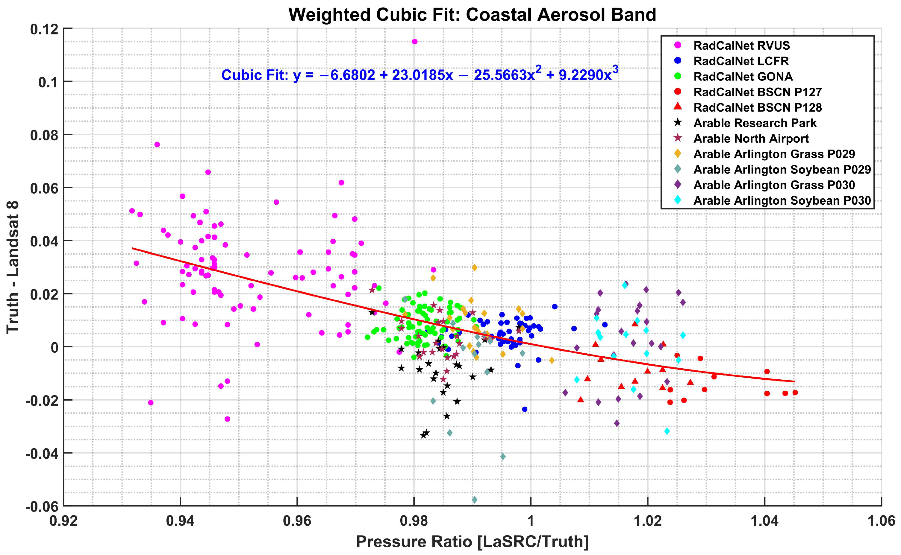
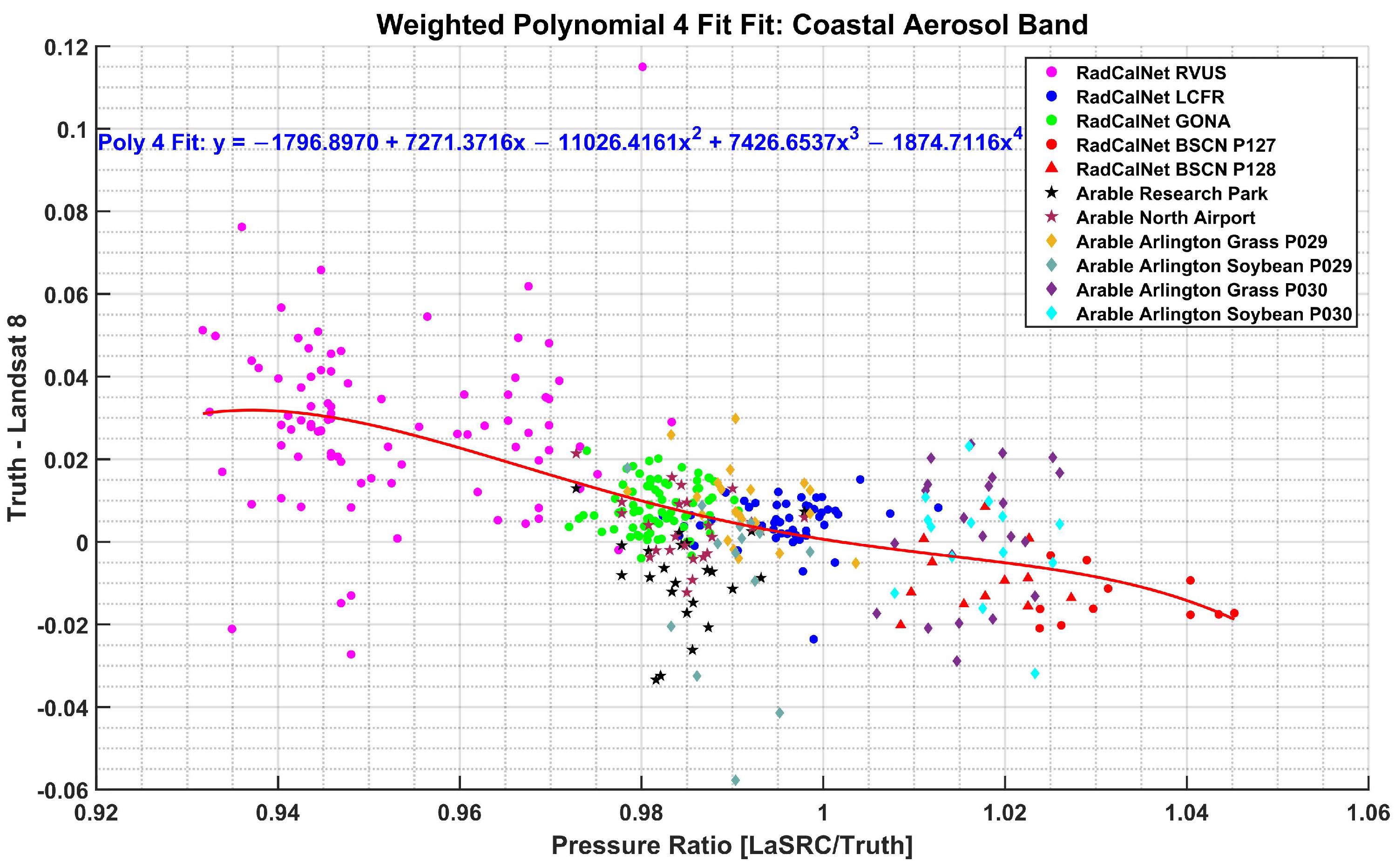
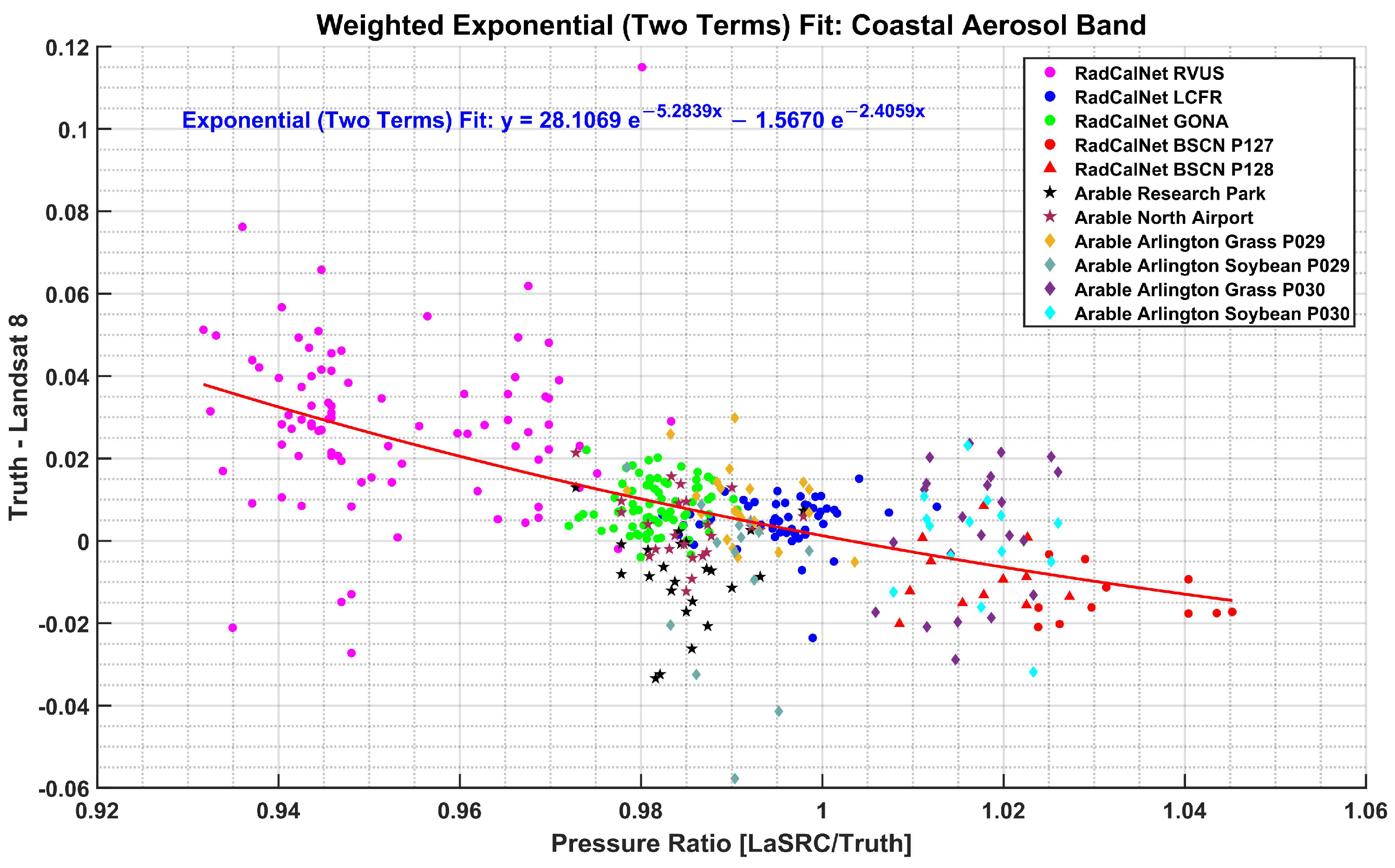
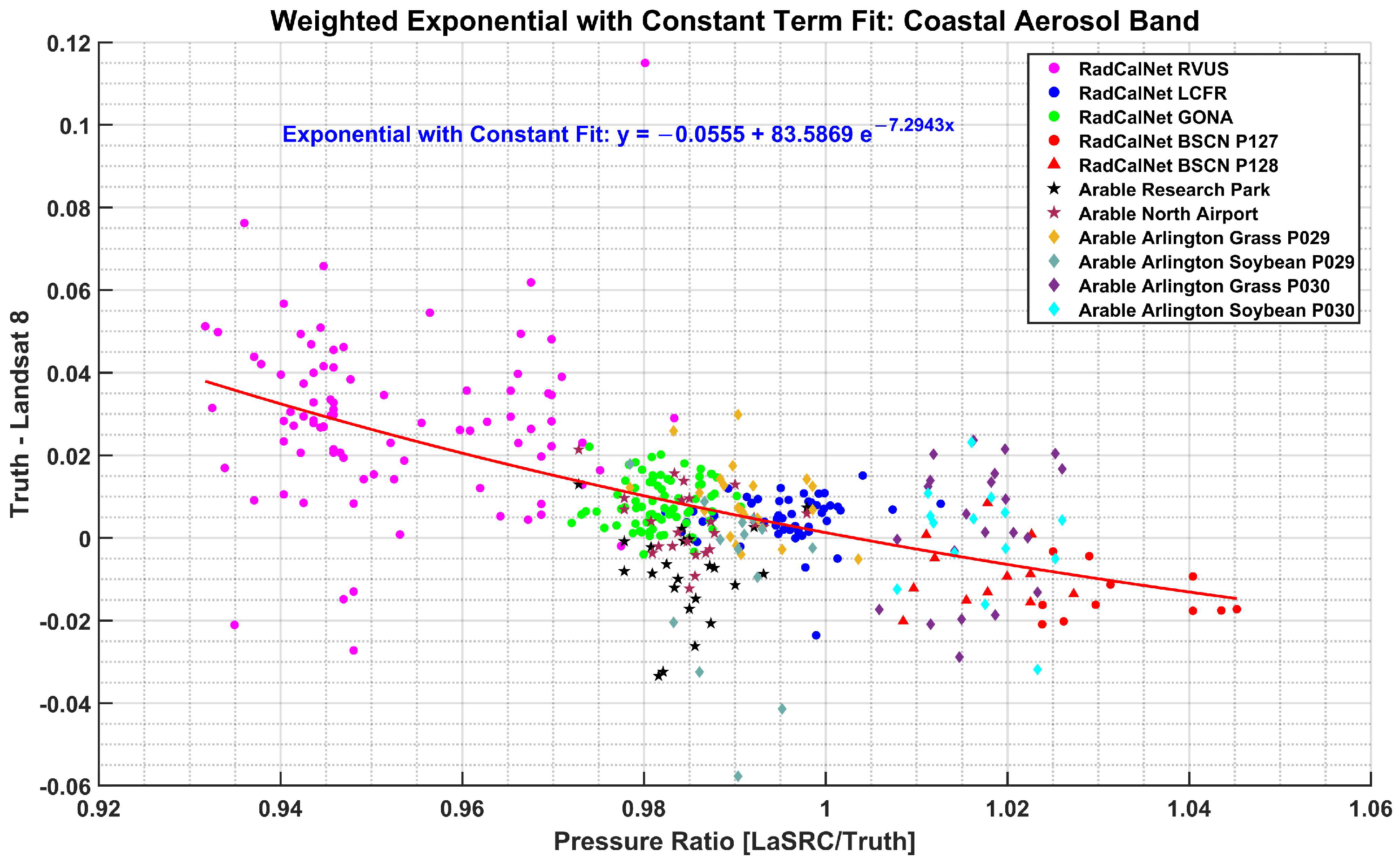
3.5. Comparison of Surface Reflectance Difference with Surface Pressure Ratio
3.6. Selection of Fit
3.7. Validation
3.7.1. Root Mean Square Deviation
3.7.2. Mean Error
3.7.3. Mean Absolute Error
4. Results
4.1. Land Surface Reflectance Code
4.1.1. Surface Reflectance Inversion
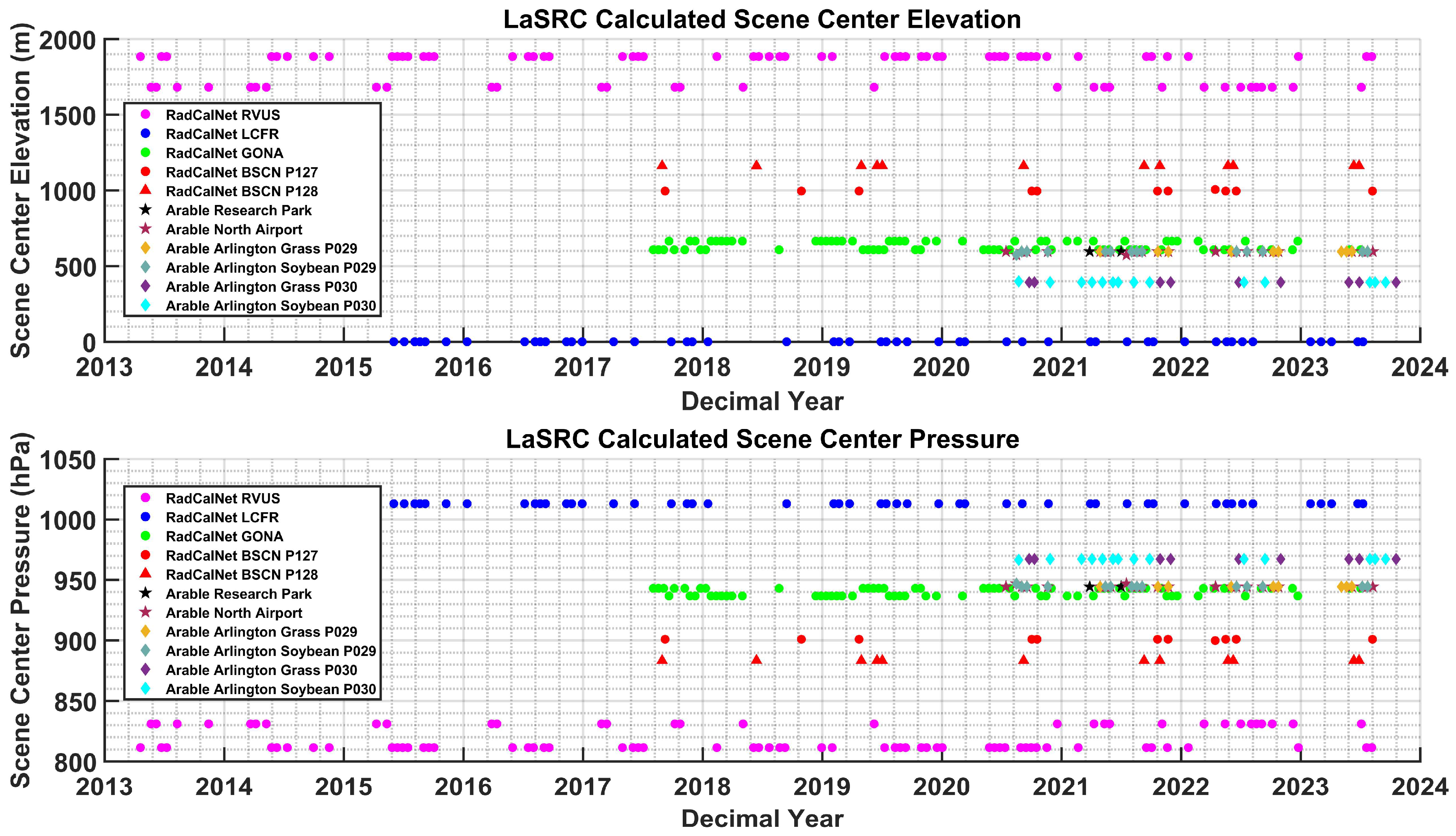
4.1.2. Calculation of LaSRC Surface Pressure for Landsat 8 Scene
4.2. Data Processing for RadCalNet Sites
4.3. Data Processing for Arable Mark 2 Sites
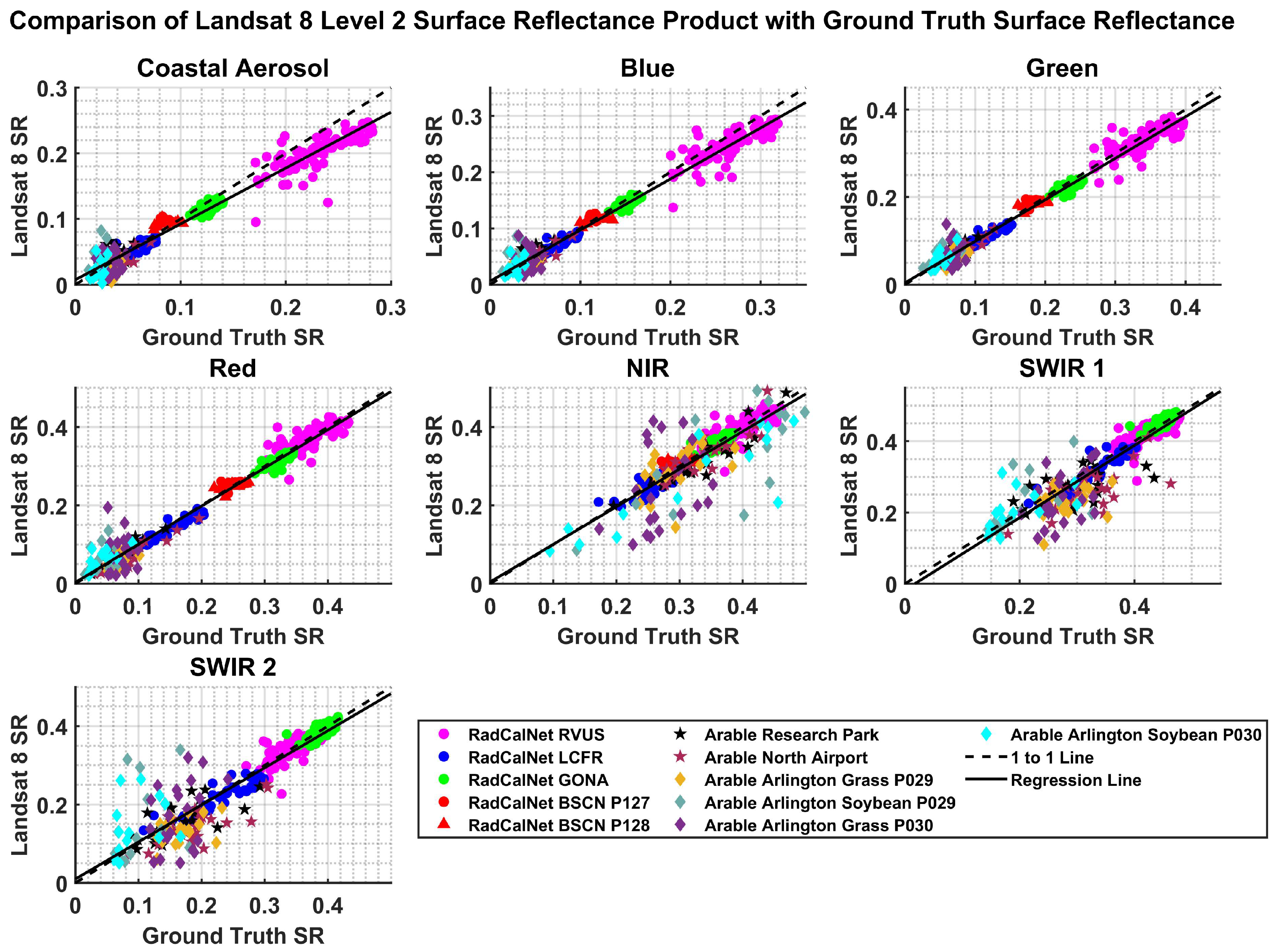
4.4. Comparison of Landsat 8 Surface Reflectance with Ground Truth Surface Reflectance
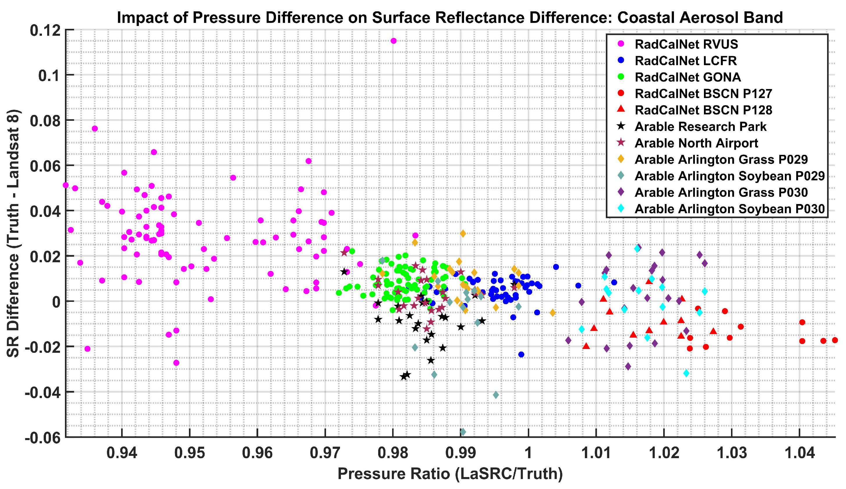
4.5. Comparison of Surface Reflectance Difference with Surface Pressure Ratio
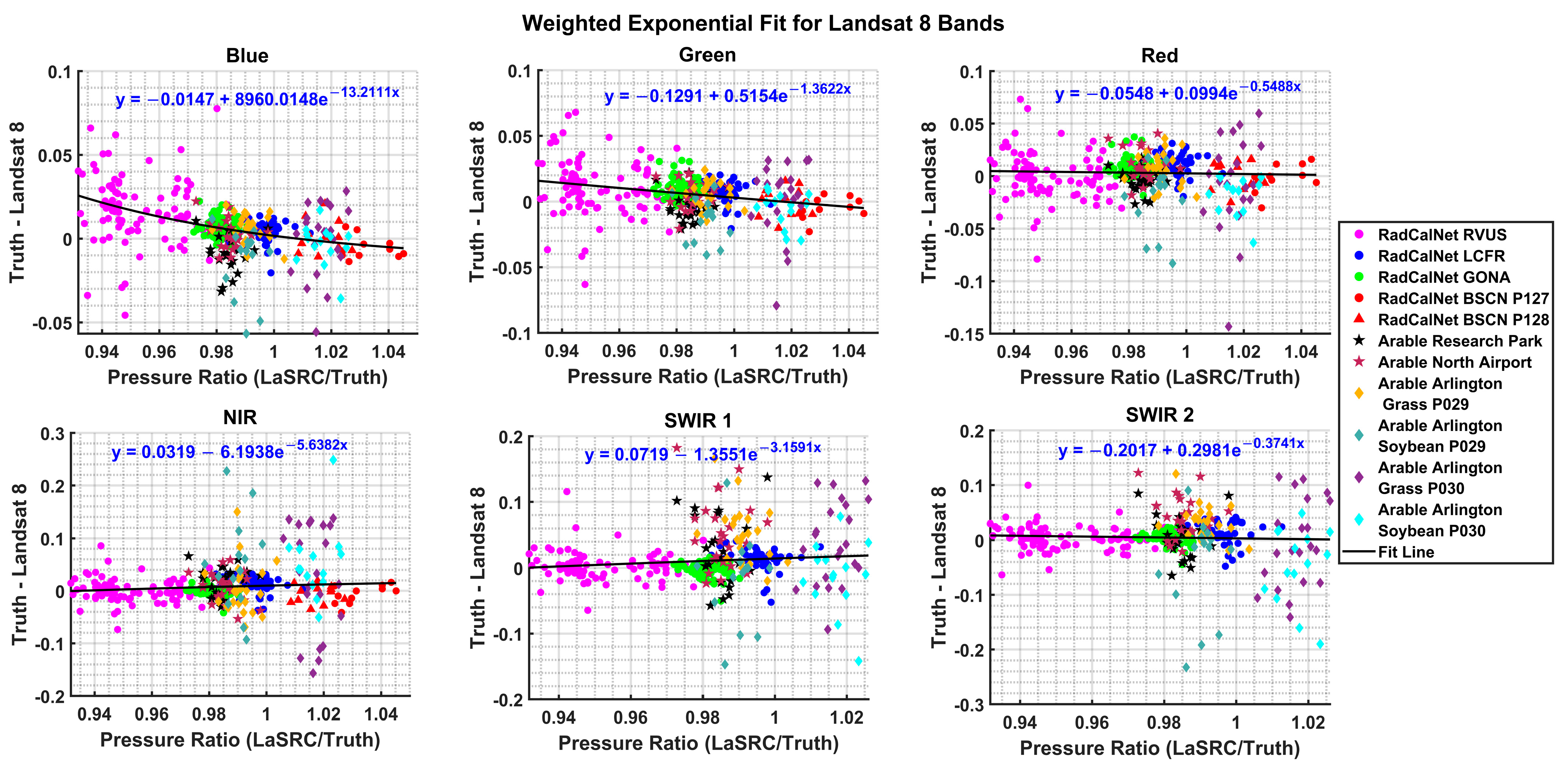
4.6. Selection of Fit
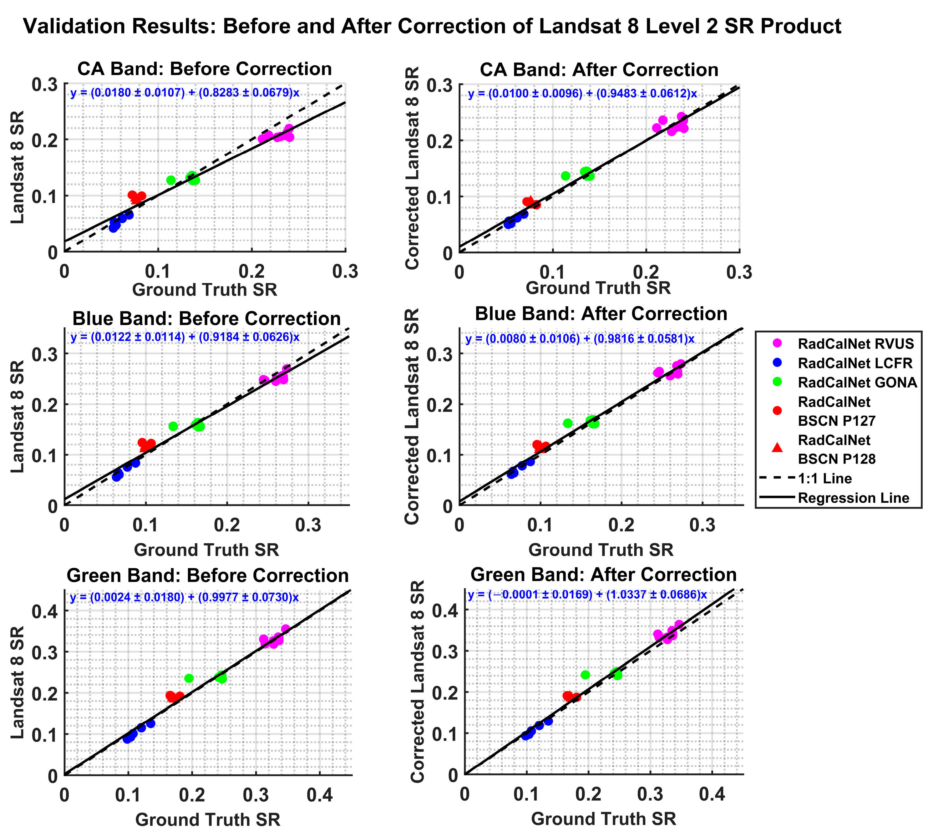
4.7. Validation
5. Discussion
5.1. Impact of Inaccurate Estimation of Surface Pressure on Landsat 8 Surface Reflectance Discrepancies
5.2. Implications and Applications of the Findings
5.3. Limitations and Future Research Directions
5.4. Long-Term Fix to the Problem
6. Conclusions
Author Contributions
Funding
Data Availability Statement
Acknowledgments
Conflicts of Interest
Appendix A

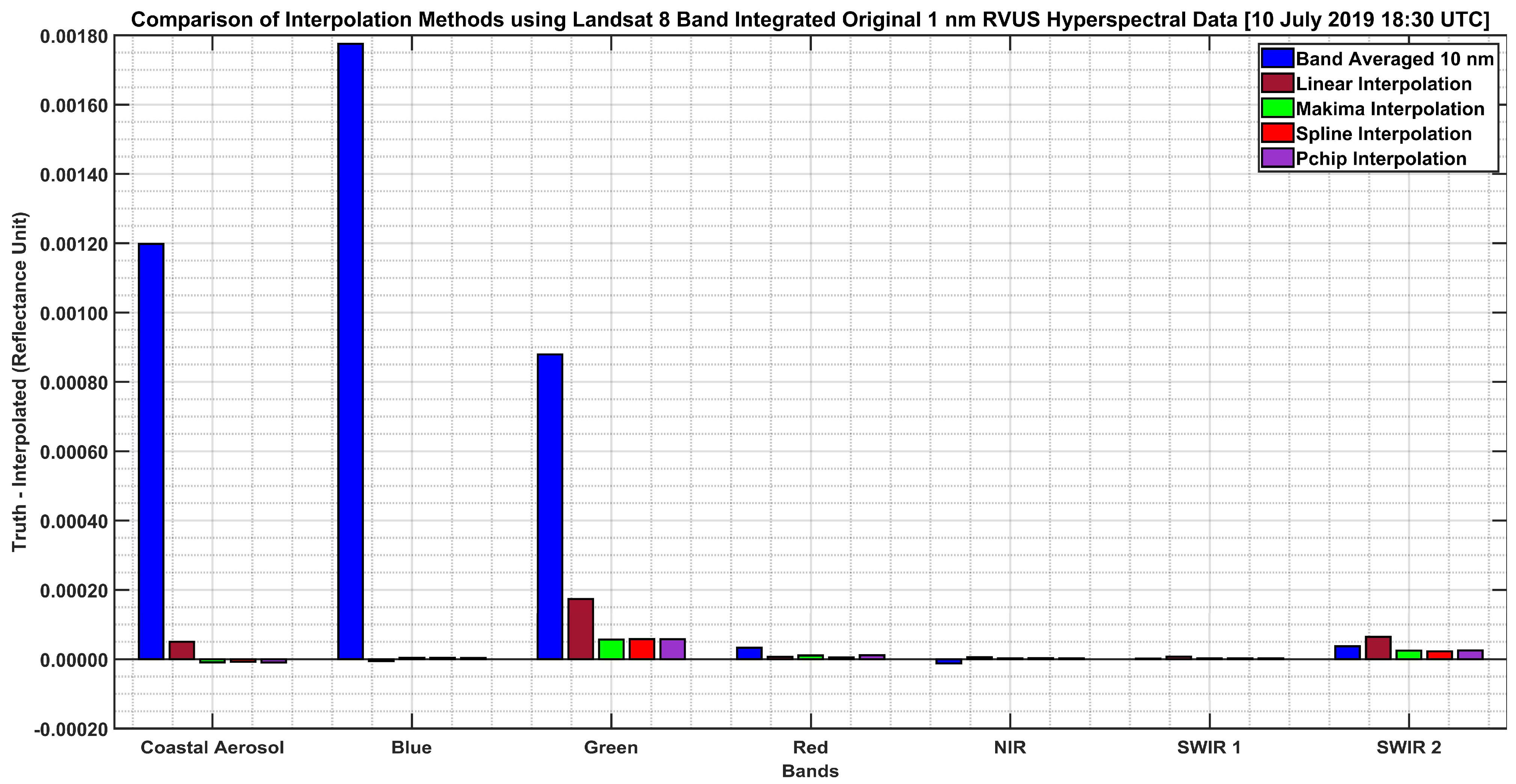
| Bands | Band-Integrated Band Averaged (10 nm) | Band-Integrated Linear (1 nm) | Band-Integrated Makima (1 nm) | Band-Integrated Spline (1 nm) | Band-Integrated PCHIP (1 nm) |
|---|---|---|---|---|---|
| Coastal Aerosol | 0.001198 | 0.000050 | −0.000009 | −0.000007 | −0.000010 |
| Blue | 0.001775 | −0.000006 | 0.000004 | 0.000004 | 0.000004 |
| Green | 0.000879 | 0.000174 | 0.000057 | 0.000058 | 0.000058 |
| Red | 0.000033 | 0.000007 | 0.000011 | 0.000005 | 0.000011 |
| NIR | −0.000012 | 0.000006 | 0.000003 | 0.000003 | 0.000003 |
| SWIR 1 | 0.000002 | 0.000007 | 0.000003 | 0.000003 | 0.000003 |
| SWIR 2 | 0.000037 | 0.000065 | 0.000025 | 0.000023 | 0.000025 |


References
- Eyre, J.; Bell, W.; Cotton, J.; English, S.; Forsythe, M.; Healy, S.; Pavelin, E. Assimilation of satellite data in numerical weather prediction. Part II: Recent years. Q. J. R. Meteorol. Soc. 2022, 148, 521–556. [Google Scholar] [CrossRef]
- Maimaitijiang, M.; Sagan, V.; Sidike, P.; Daloye, A.M.; Erkbol, H.; Fritschi, F.B. Crop Monitoring Using Satellite/UAV Data Fusion and Machine Learning. Remote Sens. 2020, 12, 1357. [Google Scholar] [CrossRef]
- Hatfield, P.; Pinter, P., Jr. Remote sensing for crop protection. Crop Prot. 1993, 12, 403–413. [Google Scholar] [CrossRef]
- Wooster, M.J.; Roberts, G.J.; Giglio, L.; Roy, D.P.; Freeborn, P.H.; Boschetti, L.; Justice, C.; Ichoku, C.; Schroeder, W.; Davies, D. Satellite remote sensing of active fires: History and current status, applications and future requirements. Remote Sens. Environ. 2021, 267, 112694. [Google Scholar] [CrossRef]
- Poland, M.P.; Lopez, T.; Wright, R.; Pavolonis, M.J. Forecasting, detecting, and tracking volcanic eruptions from space. Remote Sens. Earth Syst. Sci. 2020, 3, 55–94. [Google Scholar] [CrossRef]
- Martin, R.V. Satellite remote sensing of surface air quality. Atmos. Environ. 2008, 42, 7823–7843. [Google Scholar] [CrossRef]
- U.S. Geological Survey. Landsat 8-9 Operational Land Imager (OLI)—Thermal Infrared Sensor (TIRS) Collection 2 Level 1 (L1) Data Format Control Book (DFCB); U.S. Geological Survey: Reston, VA, USA, 2020. [Google Scholar]
- U.S. Geological Survey. Landsat 8-9 Operational Land Imager (OLI)—Thermal Infrared Sensor (TIRS) Collection 2 (C2) Level 2 (L2) Data Format Control Book (DFCB); U.S. Geological Survey: Reston, VA, USA, 2022. [Google Scholar]
- Vermote, E.; Justice, C.; Claverie, M.; Franch, B. Preliminary analysis of the performance of the Landsat 8/OLI land surface reflectance product. Remote Sens. Environ. 2016, 185, 46–56. [Google Scholar] [CrossRef]
- Wu, Z.; Snyder, G.; Vadnais, C.; Arora, R.; Babcock, M.; Stensaas, G.; Doucette, P.; Newman, T. User needs for future Landsat missions. Remote Sens. Environ. 2019, 231, 111214. [Google Scholar] [CrossRef]
- Teixeira Pinto, C.; Jing, X.; Leigh, L. Evaluation Analysis of Landsat Level-1 and Level-2 Data Products Using In Situ Measurements. Remote Sens. 2020, 12, 2597. [Google Scholar] [CrossRef]
- Badawi, M.; Helder, D.; Leigh, L.; Jing, X. Methods for Earth-Observing Satellite Surface Reflectance Validation. Remote Sens. 2019, 11, 1543. [Google Scholar] [CrossRef]
- U.S. Geological Survey. Landsat Next 2024-3005; U.S. Geological Survey: Reston, VA, USA, 2024; p. 2. [Google Scholar]
- Nazeer, M.; Ilori, C.O.; Bilal, M.; Nichol, J.E.; Wu, W.; Qiu, Z.; Gayene, B.K. Evaluation of atmospheric correction methods for low to high resolutions satellite remote sensing data. Atmos. Res. 2021, 249, 105308. [Google Scholar] [CrossRef]
- Kotchenova, S.Y.; Vermote, E.F.; Matarrese, R.; Klemm, F.J., Jr. Validation of a vector version of the 6S radiative transfer code for atmospheric correction of satellite data. Part I: Path radiance. Appl. Opt. 2006, 45, 6762–6774. [Google Scholar] [CrossRef]
- Kotchenova, S.Y.; Vermote, E.F. Validation of a vector version of the 6S radiative transfer code for atmospheric correction of satellite data. Part II. Homogeneous Lambertian and anisotropic surfaces. Appl. Opt. 2007, 46, 4455–4464. [Google Scholar] [CrossRef]
- Tanré, D.; Deroo, C.; Duhaut, P.; Herman, M.; Morcrette, J.; Perbos, J.; Deschamps, P. Technical note Description of a computer code to simulate the satellite signal in the solar spectrum: The 5S code. Int. J. Remote Sens. 1990, 11, 659–668. [Google Scholar] [CrossRef]
- Berk, A.; Anderson, G.P.; Acharya, P.K.; Bernstein, L.S.; Muratov, L.; Lee, J.; Fox, M.; Adler-Golden, S.M.; Chetwynd, J.H., Jr.; Hoke, M.L. MODTRAN5: 2006 update. In Proceedings of the Algorithms and Technologies for Multispectral, Hyperspectral, and Ultraspectral Imagery XII, Orlando, FL, USA, 8 May 2006; pp. 508–515. [Google Scholar]
- Kneizys, F.X. Users Guide to LOWTRAN 7; Air Force Geophysics Laboratory: Bedford, MA, USA, 1988; Volume 88. [Google Scholar]
- Masek, J.G.; Vermote, E.F.; Saleous, N.E.; Wolfe, R.; Hall, F.G.; Huemmrich, K.F.; Gao, F.; Kutler, J.; Lim, T.K. A Landsat Surface Reflectance Dataset for North America, 1990–2000. IEEE Geosci. Remote Sens. Lett. 2006, 3, 68–72. [Google Scholar] [CrossRef]
- Wilson, R.T. Py6S: A Python interface to the 6S radiative transfer model. Comput. Geosci. 2013, 51, 166–171. [Google Scholar] [CrossRef]
- Frantz, D. FORCE—Landsat + Sentinel-2 Analysis Ready Data and Beyond. Remote Sens. 2019, 11, 1124. [Google Scholar] [CrossRef]
- Sterckx, S.; Knaeps, E.; Adriaensen, S.; Reusen, I.; De Keukelaere, L.; Hunter, P.; Giardino, C.; Odermatt, D. OPERA: An atmospheric correction for land and water. In Proceedings of the Sentinel-3 for Science Workshop, Venice, Italy, 2–5 June 2015; pp. 3–6. [Google Scholar]
- Anderson, G.P.; Felde, G.W.; Hoke, M.L.; Ratkowski, A.J.; Cooley, T.W.; Chetwynd, J.H., Jr.; Gardner, J.; Adler-Golden, S.M.; Matthew, M.W.; Berk, A. MODTRAN4-based atmospheric correction algorithm: FLAASH (fast line-of-sight atmospheric analysis of spectral hypercubes). In Proceedings of the Algorithms and Technologies for Multispectral, Hyperspectral, and Ultraspectral Imagery VIII, Orlando, FL, USA, 2 August 2002; pp. 65–71. [Google Scholar]
- Nazeer, M.; Nichol, J.E.; Yung, Y.K. Evaluation of atmospheric correction models and Landsat surface reflectance product in an urban coastal environment. Int. J. Remote Sens. 2014, 35, 6271–6291. [Google Scholar] [CrossRef]
- KC, M.; Leigh, L.; Pinto, C.T.; Kaewmanee, M. Method of Validating Satellite Surface Reflectance Product Using Empirical Line Method. Remote Sens. 2023, 15, 2240. [Google Scholar] [CrossRef]
- Chavez, P.S., Jr. An improved dark-object subtraction technique for atmospheric scattering correction of multispectral data. Remote Sens. Environ. 1988, 24, 459–479. [Google Scholar] [CrossRef]
- Richter, R. A spatially adaptive fast atmospheric correction algorithm. Int. J. Remote Sens. 1996, 17, 1201–1214. [Google Scholar] [CrossRef]
- Hsu, N.C.; Tsay, S.C.; King, M.D.; Herman, J.R. Deep Blue Retrievals of Asian Aerosol Properties During ACE-Asia. IEEE Trans. Geosci. Remote Sens. 2006, 44, 3180–3195. [Google Scholar] [CrossRef]
- Hsu, N.C.; Jeong, M.J.; Bettenhausen, C.; Sayer, A.M.; Hansell, R.; Seftor, C.S.; Huang, J.; Tsay, S.C. Enhanced Deep Blue aerosol retrieval algorithm: The second generation. J. Geophys. Res. Atmos. 2013, 118, 9296–9315. [Google Scholar] [CrossRef]
- Kaufman, Y.J.; Wald, A.E.; Remer, L.A.; Gao, B.C.; Li, R.R.; Flynn, L. The MODIS 2.1-/spl mu/m channel-correlation with visible reflectance for use in remote sensing of aerosol. IEEE Trans. Geosci. Remote Sens. 1997, 35, 1286–1298. [Google Scholar] [CrossRef]
- Tanré, D.; Kaufman, Y.; Herman, M.; Mattoo, S. Remote sensing of aerosol properties over oceans using the MODIS/EOS spectral radiances. J. Geophys. Res. Atmos. 1997, 102, 16971–16988. [Google Scholar] [CrossRef]
- Remer, L.A.; Levy, R.C.; Mattoo, S.; Tanré, D.; Gupta, P.; Shi, Y.; Sawyer, V.; Munchak, L.A.; Zhou, Y.; Kim, M.; et al. The Dark Target Algorithm for Observing the Global Aerosol System: Past, Present, and Future. Remote Sens. 2020, 12, 2900. [Google Scholar] [CrossRef]
- Bouvet, M.; Thome, K.; Berthelot, B.; Bialek, A.; Czapla-Myers, J.; Fox, N.; Goryl, P.; Henry, P.; Ma, L.; Marcq, S.; et al. RadCalNet: A Radiometric Calibration Network for Earth Observing Imagers Operating in the Visible to Shortwave Infrared Spectral Range. Remote Sens. 2019, 11, 2401. [Google Scholar] [CrossRef]
- RadCalNet. Available online: https://www.radcalnet.org (accessed on 10 December 2024).
- Czapla-Myers, J. RadCalNet Site Description, CEOS Reference: QA4EO-WGCV-RadCalNet-RVUS-Q-v2; University of Arizona: Tucson, AZ, USA, 2022. [Google Scholar]
- Shrestha, M.; Helder, D.; Christopherson, J. DLR Earth Sensing Imaging Spectrometer (DESIS) Level 1 Product Evaluation Using RadCalNet Measurements. Remote Sens. 2021, 13, 2420. [Google Scholar] [CrossRef]
- Landier, L. RadCalNet Site Description, CEOS Reference: QA4EO-WGCV-RadCalNet-LCFR-Q-v3; CNES, Physics for Optical Measurement Service: Belin, France, 2022. [Google Scholar]
- Bialek, A.; Sinclair, M. RadCalNet Site Description, CEOS Reference: QA4EO-WGCV-RadCalNet-GONA-Q-v2; National Physical Laboratory: Hampton Road, UK, 2022. [Google Scholar]
- Marcq, S.; Meygret, A.; Bouvet, M.; Fox, N.; Greenwell, C.; Scott, B.; Berthelot, B.; Besson, B.; Guilleminot, N.; Damiri, B. New RadCalNet site at Gobabeb, Namibia: Installation of the instrumentation and first satellite calibration results. In Proceedings of the IGARSS 2018-2018 IEEE International Geoscience and Remote Sensing Symposium, Valencia, Spain, 22–27 July 2018; pp. 6444–6447. [Google Scholar]
- Ma, L. RadCalNet Site Description, CEOS Reference: QA4EO-WGCV-RadCalNet-BSCN-Q-v3; Aerospace Information Research Institute, Chinese Academy of Science: Beijing, China, 2022. [Google Scholar]
- Image Processing Lab. Available online: https://www.sdstate.edu/mccomish-electrical-engineering-computer-science/image-processing-lab (accessed on 15 December 2024).
- Pathiranage, D.S.; Leigh, L.; Pinto, C.T. Evaluation of Low-Cost Radiometer for Surface Reflectance Retrieval and Orbital Sensor’s Validation. Remote Sens. 2023, 15, 2444. [Google Scholar] [CrossRef]
- Kaufman, Y.J.; Sendra, C. Algorithm for automatic atmospheric corrections to visible and near-IR satellite imagery. Int. J. Remote Sens. 1988, 9, 1357–1381. [Google Scholar] [CrossRef]
- Crawford, C.J.; Roy, D.P.; Arab, S.; Barnes, C.; Vermote, E.; Hulley, G.; Gerace, A.; Choate, M.; Engebretson, C.; Micijevic, E. The 50-year Landsat collection 2 archive. Sci. Remote Sens. 2023, 8, 100103. [Google Scholar] [CrossRef]
- Arable Mark 2 Product Specifications. Available online: https://www.arable.com/wp-content/uploads/2021/10/Arable-Mark-2-w_-Solar-Product-Specifications-20_10.pdf (accessed on 15 December 2024).
- Arable Mark 2 Measurements. Available online: https://www.arable.com/wp-content/uploads/2021/10/Arable-Mark-2-Measurements-21_05.pdf (accessed on 15 December 2024).
- U.S. Geological Survey. Landsat 8-9 Collection 2 (C2) Level 2 Science Product (L2SP) Guide; U.S. Geological Survey: Reston, VA, USA, 2024. [Google Scholar]
- Landsat Collection 2 Atmospheric Auxiliary Data. Available online: https://www.usgs.gov/landsat-missions/landsat-collection-2-atmospheric-auxiliary-data (accessed on 13 December 2024).
- Vermote, E.F.; Tanré, D.; Deuze, J.L.; Herman, M.; Morcette, J.J. Second simulation of the satellite signal in the solar spectrum, 6S: An overview. IEEE Trans. Geosci. Remote Sens. 1997, 35, 675–686. [Google Scholar] [CrossRef]
- Earth Resources Observation and Science (EROS) Center. MODIS Fused, Collection 2 [Dataset]; U.S. Geological Survey: Reston, VA, USA, 2021. [Google Scholar] [CrossRef]
- Earth Resources Observation and Science (EROS) Center. VIIRS, Collection 2 [Dataset]; U.S. Geological Survey: Reston, VA, USA, 2023. [Google Scholar] [CrossRef]
- Kaufman, Y.J.; Tanré, D.; Remer, L.A.; Vermote, E.F.; Chu, A.; Holben, B.N. Operational remote sensing of tropospheric aerosol over land from EOS moderate resolution imaging spectroradiometer. J. Geophys. Res. Atmos. 1997, 102, 17051–17067. [Google Scholar] [CrossRef]
- Menne, M.J.; Noone, S.; Casey, N.W.; Dunn, R.H.; McNeill, S.; Kantor, D.; Thorne, P.W.; Orcutt, K.; Cunningham, S.; Risavi, N. Global Historical Climatology Network-Hourly (GHCNh), Version 1; NOAA National Centers for Environmental Information: New Orleans, LA, USA, 12–16 January 2025. [Google Scholar] [CrossRef]
- U.S. Geological Survey. Landsat 8-9 Calibration and Validation (Cal/Val) Algorithm Description Document (ADD); U.S. Geological Survey: Reston, VA, USA, 2021. [Google Scholar]
- Ott, R.; Longnecker, M. An Introduction to Statistical Methods and Data Analysis; Cengage Learning Inc.: Boston, MA, USA, 2010; p. 687. [Google Scholar]
- Concha, J.A.; Schott, J.R. Retrieval of color producing agents in Case 2 waters using Landsat 8. Remote Sens. Environ. 2016, 185, 95–107. [Google Scholar] [CrossRef]
- Algae Bloom on Lake Erie. Available online: https://earthobservatory.nasa.gov/images/84125/algae-bloom-on-lake-erie (accessed on 10 April 2025).
- Jagalingam, P.; Akshaya, B.; Hegde, A.V. Bathymetry mapping using Landsat 8 satellite imagery. Procedia Eng. 2015, 116, 560–566. [Google Scholar] [CrossRef]
- What Are the Best Landsat Spectral Bands for Use in My Research? Available online: https://www.usgs.gov/faqs/what-are-best-landsat-spectral-bands-use-my-research (accessed on 11 April 2025).


| Arable Mark 2 Sites | Center Latitude/Longitude | Land Cover | ROI Size (m) |
|---|---|---|---|
| Research Park | 44°19′16.21″N 96°45′43.08″W | Alfalfa | 60 × 90 |
| North Airport | 44°19′26.78″N 96°49′25.43″W | Grass | 90 × 60 |
| Arlington | 44°24′37.42″N 97°7′39.40″W | Grass | 90 × 30 |
| Arlington | 44°24′38.76″N 97°7′31.90″W | Soybean/Corn | 60 × 60 |
| Site | Date | LaSRC Elevation (m)/ Pressure (hPa) | Actual Elevation (m)/ Pressure (hPa) | Difference of Actual Pressure and LaSRC Pressure (hPa) |
|---|---|---|---|---|
| RVUS | 27 August 2019 | 1885/811.52 | 1435/859.00 | 47.48 |
| LCFR | 16 August 2019 | 0/1013.00 | 20/1014.92 | 1.92 |
| GONA | 27 June 2021 | 608/943.07 | 510/955.01 | 11.94 |
| BSCN Path 127 | 18 June 2022 | 996/900.99 | 1270/862.00 | −38.99 |
| BSCN Path 128 | 17 June 2022 | 1163/883.46 | 1270/864.00 | −19.46 |
| Arable Research Park | 23 November 2021 | 596/944.40 | 502.3/946.38 | 1.98 |
| Arable North Airport | 23 November 2021 | 596/944.40 | 502.3/946.38 | 1.98 |
| Arable Arlington Grass Path 029 | 7 September 2022 | 596/944.40 | 548.9/957.19 | 12.79 |
| Arable Arlington Soybean Path 029 | 7 September 2022 | 596/944.40 | 548.9/957.19 | 12.79 |
| Arable Arlington Grass Path 030 | 12 July 2022 | 393/967.23 | 548.9/953.72 | −13.51 |
| Arable Arlington Soybean Path 030 | 12 July 2022 | 393/967.23 | 548.9/953.72 | −13.51 |
| Site | Mean Difference Between Actual Pressure and LaSRC Pressure (hPa) | Mean Difference Between Actual SR and Landsat 8 SR (Reflectance Unit) |
|---|---|---|
| RVUS | 41.12 ± 11.12 | 0.0285 ± 0.0202 |
| LCFR | 4.55 ± 6.01 | 0.0048 ± 0.0060 |
| GONA | 17.37 ± 3.81 | 0.0084 ± 0.0059 |
| BSCN Path 127 | −28.38 ± 6.93 | −0.0140 ± 0.0061 |
| BSCN Path 128 | −14.97 ± 5.13 | −0.0085 ± 0.0083 |
| Arable Research Park | 14.68 ± 5.26 | −0.0088 ± 0.0116 |
| Arable North Airport | 14.18 ± 5.21 | 0.0034 ± 0.0079 |
| Arable Arlington Grass Path 029 | 8.39 ± 5.12 | 0.0084 ± 0.0088 |
| Arable Arlington Soybean Path 029 | 9.80 ± 4.86 | −0.0092 ± 0.0213 |
| Arable Arlington Grass Path 030 | −15.78 ± 4.99 | 0.0024 ± 0.0160 |
| Arable Arlington Soybean Path 030 | −16.19 ± 5.11 | −0.0003 ± 0.0134 |
| Fit Type | Residual Mean Error (Reflectance Unit) | Residual Standard Deviation (Reflectance Unit) |
|---|---|---|
| Linear | −0.0007 | 0.0150 |
| Quadratic | −0.0005 | 0.0149 |
| Cubic | −0.0005 | 0.0149 |
| Polynomial 4 | −0.0004 | 0.0148 |
| Logarithmic | −0.0006 | 0.0150 |
| Two Exponential Terms | −0.0005 | 0.0149 |
| Exponential with Constant | −0.0005 | 0.0149 |
| Landsat 8 Bands | F-Statistic | p-Value | Significance at α = 0.01 |
|---|---|---|---|
| Coastal Aerosol | 124 | 1.79 × 10−41 | Significant |
| Blue | 97.6 | 1.68 × 10⁻²⁰ | Significant |
| Green | 15.7 | 3.02 × 10⁻⁷ | Significant |
| Red | 0.311 | 0.733 | Not significant |
| NIR | 1.46 | 0.234 | Not significant |
| SWIR 1 | 2.12 | 0.122 | Not significant |
| SWIR 2 | 0.376 | 0.687 | Not significant |
| Landsat 8 Bands | a | b | c |
|---|---|---|---|
| Coastal Aerosol | −0.0555 | 83.5869 | −7.2943 |
| Blue | −0.0147 | 8960.0148 | −13.2111 |
| Green | −0.1291 | 0.5154 | −1.3622 |
| Landsat 8 Bands | Before Correction | After Correction | ||||
|---|---|---|---|---|---|---|
| RMSD | ME | MAE | RMSD | ME | MAE | |
| Coastal Aerosol | 0.0203 | 0.0087 | 0.0145 | 0.0149 | −0.0005 | 0.0101 |
| Blue | 0.0169 | 0.0057 | 0.0120 | 0.0145 | −0.0009 | 0.0095 |
| Green | 0.0172 | 0.0054 | 0.0128 | 0.0158 | −0.0005 | 0.0111 |
| Landsat 8 Bands | RadCalNet Sites | RMSD | ME | MAE |
|---|---|---|---|---|
| Coastal Aerosol Band (Before Correction) | RVUS | 0.0241 | 0.0226 | 0.0226 |
| LCFR | 0.0060 | 0.0049 | 0.0049 | |
| GONA | 0.0086 | 0.0022 | 0.0067 | |
| BSCN P127 | 0.0235 | −0.0228 | 0.0228 | |
| BSCN P128 | 0.0162 | −0.0159 | 0.0159 | |
| All Sites Combined | 0.0173 | 0.0061 | 0.0140 | |
| Coastal Aerosol Band (After Correction) | RVUS | 0.0122 | 0.0029 | 0.0111 |
| LCFR | 0.0022 | 0.0006 | 0.0017 | |
| GONA | 0.0113 | −0.0075 | 0.0089 | |
| BSCN P127 | 0.0129 | −0.0103 | 0.0103 | |
| BSCN P128 | 0.0115 | −0.0110 | 0.0110 | |
| All Sites Combined | 0.0106 | −0.0027 | 0.0084 | |
| Blue Band (Before Correction) | RVUS | 0.0123 | 0.0095 | 0.0103 |
| LCFR | 0.0051 | 0.0044 | 0.0044 | |
| GONA | 0.0110 | 0.0007 | 0.0081 | |
| BSCN P127 | 0.0228 | −0.0219 | 0.0219 | |
| BSCN P128 | 0.0148 | −0.0147 | 0.0147 | |
| All Sites Combined | 0.0124 | 0.0013 | 0.0098 | |
| Blue Band (After Correction) | RVUS | 0.0104 | −0.0032 | 0.0090 |
| LCFR | 0.0020 | 0.0012 | 0.0017 | |
| GONA | 0.0124 | −0.0056 | 0.0088 | |
| BSCN P127 | 0.0185 | −0.0171 | 0.0171 | |
| BSCN P128 | 0.0134 | −0.0132 | 0.0132 | |
| All Sites Combined | 0.0111 | −0.0050 | 0.0084 | |
| Green Band (Before Correction) | RVUS | 0.0086 | −0.0014 | 0.0067 |
| LCFR | 0.0087 | 0.0084 | 0.0084 | |
| GONA | 0.0183 | −0.0007 | 0.0127 | |
| BSCN P127 | 0.0214 | −0.0196 | 0.0196 | |
| BSCN P128 | 0.0154 | −0.0151 | 0.0151 | |
| All Sites Combined | 0.0138 | −0.0019 | 0.0105 | |
| Green Band (After Correction) | RVUS | 0.0147 | −0.0114 | 0.0115 |
| LCFR | 0.0046 | 0.0042 | 0.0042 | |
| GONA | 0.0196 | −0.0071 | 0.0119 | |
| BSCN P127 | 0.0186 | −0.0159 | 0.0159 | |
| BSCN P128 | 0.0155 | −0.0152 | 0.0152 | |
| All Sites Combined | 0.0152 | −0.0076 | 0.0107 |
Disclaimer/Publisher’s Note: The statements, opinions and data contained in all publications are solely those of the individual author(s) and contributor(s) and not of MDPI and/or the editor(s). MDPI and/or the editor(s) disclaim responsibility for any injury to people or property resulting from any ideas, methods, instructions or products referred to in the content. |
© 2025 by the authors. Licensee MDPI, Basel, Switzerland. This article is an open access article distributed under the terms and conditions of the Creative Commons Attribution (CC BY) license (https://creativecommons.org/licenses/by/4.0/).
Share and Cite
Adhikari, S.; Leigh, L.; Pathiranage, D.S. Pressure-Related Discrepancies in Landsat 8 Level 2 Collection 2 Surface Reflectance Products and Their Correction. Remote Sens. 2025, 17, 1676. https://doi.org/10.3390/rs17101676
Adhikari S, Leigh L, Pathiranage DS. Pressure-Related Discrepancies in Landsat 8 Level 2 Collection 2 Surface Reflectance Products and Their Correction. Remote Sensing. 2025; 17(10):1676. https://doi.org/10.3390/rs17101676
Chicago/Turabian StyleAdhikari, Santosh, Larry Leigh, and Dinithi Siriwardana Pathiranage. 2025. "Pressure-Related Discrepancies in Landsat 8 Level 2 Collection 2 Surface Reflectance Products and Their Correction" Remote Sensing 17, no. 10: 1676. https://doi.org/10.3390/rs17101676
APA StyleAdhikari, S., Leigh, L., & Pathiranage, D. S. (2025). Pressure-Related Discrepancies in Landsat 8 Level 2 Collection 2 Surface Reflectance Products and Their Correction. Remote Sensing, 17(10), 1676. https://doi.org/10.3390/rs17101676