Article

GNSS Precipitable Water Vapor Prediction for Hong Kong Based on ICEEMDAN-SE-LSTM-ARIMA Hybrid Model

1
State Key Laboratory of Geohazard Prevention and Geoenvironment Protection, Chengdu 610059, China
2
College of Earth and Planetary Science, Chengdu University of Technology, Chengdu 610059, China
*
Author to whom correspondence should be addressed.
Remote Sens. 2025, 17(10), 1675; https://doi.org/10.3390/rs17101675
Submission received: 25 March 2025 / Revised: 30 April 2025 / Accepted: 8 May 2025 / Published: 9 May 2025

Abstract

:
Accurate prediction of Global Navigation Satellite System-derived precipitable water vapor (GNSS-PWV), which is a crucial indicator for climate change monitoring, holds significant scientific value for climate disaster prevention and mitigation. In the study of GNSS-PWV prediction, the complete ensemble empirical mode decomposition with adaptive noise (CEEMDAN) algorithm within a decomposition–integration framework effectively addresses the non-stationarity and complexity of PWV sequences, enhancing prediction accuracy. However, residual noise and pseudo-modes from decomposition can distort signals, reducing the predictor system’s reliability. Additionally, independent modeling of all decomposed components decreases computational efficiency. To address these challenges, this paper proposes a hybrid model combining the improved complete ensemble empirical mode decomposition with adaptive noise (ICEEMDAN), autoregressive integrated moving average (ARIMA), and long short-term memory (LSTM) networks. Enhanced by local mean optimization and adaptive noise regulation, the ICEEMDAN algorithm effectively suppresses pseudo-modes and minimizes residual noise, enabling its decomposed intrinsic mode functions (IMFs) to more accurately capture the multi-scale features of GNSS-PWV. Sample entropy (SE) is used to quantify the complexity of IMFs, and components with similar entropy values are reconstructed into the following three sub-sequences: high-frequency, low-frequency, and trend. This process significantly reduces modeling complexity and improves computational efficiency. We propose different modeling strategies tailored to the dynamics of various subsequences. For the nonlinear and non-stationary high-frequency components, the LSTM network is used to effectively capture their complex patterns. The LSTM’s gating mechanism and memory cell design proficiently address the long-term dependency issue. For the stationary and weakly nonlinear low-frequency and trend components, linear patterns are extracted using ARIMA. Differencing eliminates trends and moving average operations capture random fluctuations, effectively addressing periodicity and trends in the time series. Finally, the prediction results of the three components are linearly combined to obtain the final prediction value. To validate the model performance, experiments were conducted using measured GNSS-PWV data from several stations in Hong Kong. The results demonstrate that the proposed model reduces the root mean square error by 56.81%, 37.91%, and 13.58% at the 1 h scale compared to the LSTM, EMD-LSTM, and ICEEMDAN-SE-LSTM benchmark models, respectively. Furthermore, it exhibits strong robustness in cross-month forecasts (accounting for seasonal influences) and multi-step predictions over the 1–6 h period. By improving the accuracy and efficiency of PWV predictions, this model provides reliable technical support for the real-time monitoring and early warning of extreme weather events in Hong Kong while offering a universal methodological reference for multi-scale modeling of geophysical parameters.

1. Introduction

Precipitable water vapor (PWV) is the sum of the mass of water vapor in the vertical atmospheric column from the ground to the top of the atmosphere, and as one of the key parameters for measuring extreme weather events such as typhoons, heavy rains, and droughts it plays a crucial role in the evolution of the climate system and the process of energy transfer [1,2,3]. Compared with traditional observation methods, GNSS-PWV has several advantages as it is all-weather, highly accurate, and low-cost. These advantages contribute to better monitoring and assessment of changes in weather systems and ultimately improve the quality of data used in regional climate studies [4,5]. In addition, Hong Kong’s geographical location is unique in that it is subject to the southeast monsoon from the Pacific Ocean in summer and the dry northeast monsoon from inland areas in winter. This alternation of monsoon winds leads to unique and complex characteristics of PWV in terms of spatial distribution and temporal changes, which in turn increases the risk of extreme weather events [6]. GNSS-PWV is an effective tool for studying extreme weather, revealing multi-scale coupling information of weather systems in its time series [7]. High-precision modeling predictions utilizing GNSS-PWV time series have become crucial for disaster prevention and mitigation in urban areas like Hong Kong. Accurate predictions significantly impact climate research and weather forecasting [8].
Several complex environmental factors contribute to the instability, multi-scale nature, and nonlinear characteristics of GNSS-PWV, making accurate predictions challenging. GNSS-PWV prediction models are categorized into the following three main types: traditional linear, deep learning, and combinatorial [9]. Although the traditional linear model can fit the linear part of the PWV series better [10,11,12], it is difficult to deal with the nonlinear relationship of PWV, which affects the prediction accuracy [13]. The rapid advancement of computer technology and the rise in high-performance GPUs have led to increased interest from researchers, both domestically and internationally, in using data-driven deep learning methods for predicting PWV [14,15,16,17]. Data-driven deep learning models have greatly enhanced predictive capabilities compared to traditional linear models [18,19]. However, GNSS-PWV sequences are highly complex and typically consist of multiple components, including trends, seasonal variations, and random fluctuations. Capturing this intricate, multi-component nature poses a significant challenge that limits further advancements in the accuracy of GNSS-PWV predictions [20].
Researchers have introduced an innovative strategy called decomposition integration, which has become a mainstream approach to enhancing the accuracy of GNSS-PWV predictions. This method involves extracting multi-scale subsequences through signal decomposition algorithms and constructing a hybrid prediction framework for targeted modeling [21,22,23]. It is important to note that the effectiveness of the decomposition–integration strategy largely relies on the performance of the signal decomposition algorithm used. Existing decomposition algorithms such as VMD, WT, and EMD have deficiencies such as a sensitivity to initial values, difficulty in adapting to non-stationary characteristics [24,25,26], and endpoint effects. While CEEMDAN solves the endpoint effect problem to a certain extent, research has indicated that the CEEMDAN can accumulate residual noise and interference from pseudo-modes during its iterative process [27]. This accumulation may distort the modal information and reduce the signal-to-noise ratio, ultimately compromising the generalization ability of subsequent prediction models. More importantly, the existing decomposition–integration framework faces the “accuracy–efficiency” trade-off paradox. On the one hand, the independent prediction and weighted superposition of decomposed components guarantees the prediction accuracy but significantly increases the model training time, which leads to inefficiency [28]; on the other hand, only combining decomposed components into high-frequency and low-frequency terms without modeling and estimating the trend terms, which contain the characteristics of the data’s long-term evolution, improves the prediction efficiency but limits the prediction accuracy [29]. Ultimately, these phenomena are due to the lack of noise robust adaptive GNSS-PWV decomposition algorithms and physically meaningful subsequence reconstruction criteria. Therefore, solving the pseudo-modal and residual noise problems of the CEEMDAN algorithm while improving the prediction efficiency and accuracy of GNSS-PWV remains an important challenge to be overcome.
To this end, we construct a hybrid ICEEMDAN-sample entropy (SE)-LSTM-ARIMA (IS-LA) model. By decomposing the data, reconstructing the features, and integrating the results, effective modeling of complex sequences is achieved. Its innovative contributions are reflected in the following three aspects: (1) This paper innovatively proposes the IS-LA hybrid model applied to GNSS-PWV prediction, which solves the pseudo-modal and residual noise problems when the CEEMDAN algorithm decomposes the complex PWV data through the optimization of the local mean estimation and the dynamic adjustment mechanism of the noise energy and improves the physical fidelity of the decomposition of PWV signals. (2) Based on the SE to quantize the subsequence complexity, the threshold method is used to reconstruct the isomorphic modes into high-frequency, low-frequency, and trend components, which, on the one hand, reduces the number of prediction times and improves the prediction efficiency, and on the other hand distinguishes the components of different complexity and subsequently establishes a more targeted and reasonable prediction model to help improve the prediction accuracy. (3) The LSTM-ARIMA parallel prediction framework is constructed, and based on the results of the augmented Dickey–Fuller test (ADF) and the Brock–Dechert–Scheinkman test (BDS), LSTM deep learning is used to model the non-stationary high-frequency components while ARIMA is used to parametrically estimate the low-frequency terms with a low degree of nonlinearity and the trend terms, so as to realize the synergistic optimization of “data-driven + model-driven”.

2. Materials and Methods

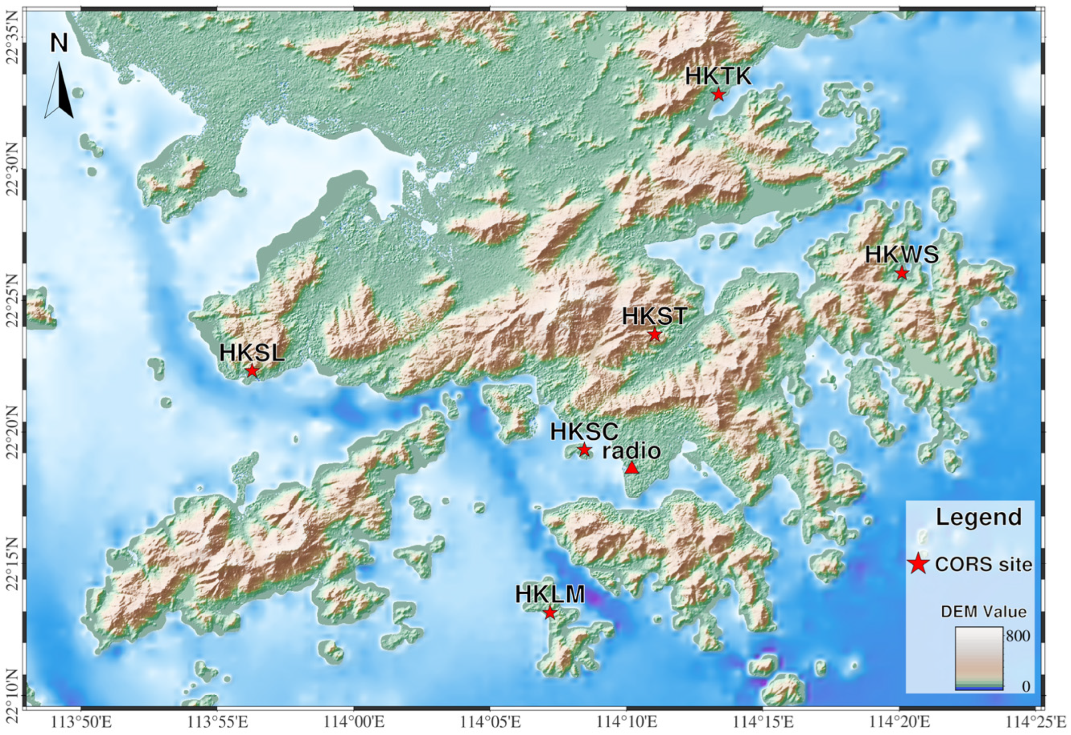
2.1. Study Area and Data Description

With the rapid development of GNSS, many cities have established dense networks of continuously operating reference stations (CORSs). These networks provide a rich data source for GNSS water vapor remote sensing. In this study, we selected the observation data from 1 January to 31 December 2022 from the Hong Kong positioning reference station network (https://www.geodetic.gov.hk, accessed on 1 April 2024). We focus on six CORSs (HKLM, HKSC, HKSL, HKST, HKTK, and HKWS) in Hong Kong with different orientations and the least missing data, and their specific missing data rates are shown in Appendix A Table A1. These stations generally cover the whole Hong Kong region and help us understand the overall distribution of GNSS-PWV in the region. The sounding station observations were provided by the University of Wyoming, USA (http://weather.uwyo.edu/upperair/, accessed on 20 April 2024). Figure 1 illustrates the distribution of the selected CORSs and sounding stations.
In advance, GNSS observation files of 6 stations in 2022 are processed into hourly GNSS PWV data by GAMIT. GNSS signals are affected by the atmosphere, which can result in signal delay including ionospheric delay and tropospheric delay. zenith tropospheric delay (ZTD) consists of two components: zenith hydrostatic delay (ZHD) and zenith wet delay (ZWD). ZHD, which is caused by dry air in the atmosphere, accounts for approximately 90% of ZTD The zenith wet delay, resulting from atmospheric water vapor, makes up 10% of the total zenith delay. The transformation relationship between PWV and ZWD is as follows [30]:
Z T D = Z H D + Z W D
P W V = π × Z W D
π = 10 6 ρ W × R V × K 3 T m + K 2
where π represents the dimensionless conversion factor of GNSS-PWV, ρ w denotes the liquid water density (unit: kg / m 3 ), R v denotes the water vapor gas constant (unit: J / ( kg K ) ), k 2 is an atmospheric humidity constant with a value of 71.98 (unit: K / hpa ), k 3 represents the atmospheric refraction parameters with empirical values of 3.754 × 10 5 (unit: K 2 / hpa ), and T m denotes the weighted average temperature (unit: K ).

2.2. Data Preprocessing

This paper evaluates and verifies the accuracy and usability of inverse PWV from GNSS data based on the distribution characteristics of the sounding stations in Hong Kong. The HKSC station, which is only 2 km away from the sounding station, is selected for the accuracy analysis, but due to the inconsistency in the temporal resolution of the two data sources, the values of GNSS-PWV and Radio-PWV at 00:00 and 12:00 UTC in which the time span is the same, are compared with those at the time of acquisition of the sounding data to ensure the consistency of the observation time between the two data. Time coordinated (UTC), the values of GNSS-PWV and Radio-PWV at time 0 and 12 are compared to ensure that the observation time between the two data is the same and there is no precision deviation due to the time span. The precision statistics of the two are shown in Table 1.
According to the data in Table 1, it can be seen that the measurements of GNSS-PWV and Radio-PWV from HKSC stations show high accuracy and consistency at both 12 and 0 moments. Most of the Radio-PWV is slightly lower than the GNSS-PWV, but there is a slight bias in individual places due to the end effect of obtaining CORS data and the inconsistency in the location and elevation of the sounding station and the CORS. Although there are some deviations, the maximum and minimum deviations are within reasonable ranges and the average deviations are small, with the root mean square errors all less than 3.1 mm and the correlation coefficients greater than 0.98, which indicates that the measurements of the two methods are in good agreement. In addition, the average deviation at 12 moments is slightly higher than that at 0 moments, which may be related to the change in atmospheric conditions at different moments of the day, such as the strongest solar radiation at noon which promotes evaporation and atmospheric convective activities, and the solar radiation at midnight which is almost zero and weakens the convective activities. To visualize the correlation between GNSS-PWV and Radio-PWV, the scatter plot of the two is shown in Figure 2.
Figure 2 shows the correlation between GNSS-PWV and Radio-PWV at different moments, and the data are primarily distributed on both sides of the fitted straight line and the correlation coefficients between Radio-PWV and GNSS-PWV at the moments of 0 and 12 are both greater than 0.95. It should be noted that although the airborne observation data and the observation results of the CORS are adjusted to the same height in the elevation direction there are still spatial differences in the horizontal position, which may lead to the inconsistency of the precipitable water vapor content obtained by the two techniques. There are still spatial differences in the horizontal position, which may lead to inconsistency in the precipitable water vapor content obtained by the two techniques. In general, the GNSS-PWV and Radio-PWV detected by two independent means have a high consistency in changes, and the reliability and accuracy of the GNSS-PWV data are high enough to be used in the next PWV prediction study.

3. Methodology

3.1. IS-LA Model Construction

This paper introduces an innovative hybrid prediction model, IS-LA, which combines the methods of ICEEMDAN, SE, LSTM, and ARIMA. The goal is to address the limitations of existing GNSS-PWV prediction models, thereby enhancing both the accuracy and efficiency of GNSS-PWV predictions. This model enables precise modeling and forecasting of water vapor data through the synergistic effects of the incorporated methods.
To address the issues of residual noise and pseudo-modal problems in the CEEMDAN algorithm used for decomposing GNSS-PWV sequences, this paper introduces the ICEEMDAN method [31]. This approach enhances CEEMDAN by effectively reducing modal aliasing and minimizing the occurrence of pseudo-modals. It accomplishes this through a dynamic injection mechanism for adaptive noise and an optimization strategy based on local mean estimation. Additionally, it features the adaptive adjustment of noise energy as the order increases. Specifically, for the extraction process of each order mode, the local mean estimation of the adaptive noise is performed for the adaptive noise containing, and the K order mode I M F K is defined as follows:
I M F K = E i M k 1 i t M ˜ k t
where M k 1 i t is the result of the k 1 decomposition of the i order residuals with the addition of Gaussian white noise, M ˜ k t is the local mean ensemble averaging, and E denotes the expectation operation under multiple realizations. This strategy significantly suppresses mode aliasing and pseudo-modal generation through dynamic noise injection and mean value optimization.
By introducing an adaptive coefficient β k , which increases the noise energy with the decomposition order, the separation efficiency of the high-frequency noise from the low-frequency trend is equalized as follows:
β k = σ r k 1 ε k 1
where σ r k 1 represents the standard deviation of the residual from the previous decomposition stage and ε is a decay factor introduced to control the noise energy increment across decomposition stages.
Although the ICEEMDAN algorithm significantly improves the decomposition accuracy of the GNSS-PWV data through local mean optimization and adaptive noise adjustment, each component is modeled separately, which significantly increases the arithmetic burden; for this reason, this paper uses the sample entropy algorithm to accurately quantify the degree of complexity and irregularity of the time series, according to the value of the SE and the characteristics of the data presented by each component. Based on the SE value and the characteristics of each data component, we categorize the components as follows: Those with an SE value greater than 1 are classified as high-frequency terms with high complexity and low amplitude. Components with an SE value close to 0 and showing a clear trend are classified as trend terms. The remaining components are categorized as low-frequency terms. Using reconstructed data for modeling and prediction, rather than separately modeling each component, can enhance prediction accuracy and efficiency. The corresponding formula for this process is as follows:
S a m p E n m , r = ln A m r B m r
where m denotes the embedding dimension used to reconstruct the phase space of the time series, r is the similarity tolerance threshold that determines the maximum distance between template vectors for them to be considered similar, and A m r and B m r are the counts of template vector pairs meeting the distance threshold in m + 1-dimensional and m-dimensional spaces, respectively. This reduces the modeling times from X to only 3, significantly improving computational efficiency and establishing a foundation for targeted model selection.
The reconstructed high-frequency, low-frequency, and trend components show significant differences in their characteristics. These distinct features make it challenging for a single model to accurately capture the dynamic behavior of all components simultaneously. Therefore, choosing the right prediction models for the different components enhances prediction accuracy. In this paper, we quantitatively analyze the statistical characteristics of each element using the ADF and the BDS. This analysis aims to provide a scientific basis for selecting appropriate models. Specifically, the ADF is applied to each reconstructed component to assess its stationarity and the data are basically distributed on both sides of the fitted straight line. If the ADF statistic is smaller than the critical value at the specified significance level (5%) then we reject the null hypothesis and conclude that the series is smooth, otherwise it is considered non-smooth. Meanwhile, the BDS was used to quantify the nonlinear characteristics of the components, whose statistics W B D S obey the χ 2 distribution and when W B D S > χ 1 α 2 m they indicate a significant nonlinear structure in the sequence. Based on the above test results, the model selection strategy is as follows: for the high-frequency components that pass the BDS and the ADF shows non-stationarity, the LSTM model is used for modeling; while for the low-frequency and trend components that pass the ADF and fail the BDS, the ARIMA (p,d,q) model is used. The LSTM dynamically modulates the information flow through the gating mechanism of the input gate, the forgetting gate, and the output gate. Information flow is mathematically expressed as follows:
f t = σ ( W f [ h t 1 , x t ] + b f ) i t = σ ( W i [ h t 1 , x t ] + b i ) C ˜ t = tanh ( W C [ h t 1 , x t ] + b C ) C t = f t C t 1 + i t C ˜ t o t = σ ( W o [ h t 1 , x t ] + b o ) h t = o t tanh ( C t )
where w represents the weights and σ represents the sigmoid function. The structure maintains long-term dependencies using a memory unit and identifies key features through a gating unit. This approach effectively captures chaotic fluctuations and nonlinear characteristics of high-frequency components while preventing the gradient vanishing problem commonly found in traditional recurrent neural networks (RNNs) [32]. During the optimization process of the LSTM model, the Adam algorithm is used to adjust the internal training parameters, and a dropout layer is incorporated to mitigate overfitting. The maximum number of training epochs is 169, the output window size is 1, and a gradient threshold constraint of 1 is applied to prevent gradient explosion. The initial learning rate is set to 0.0064, and if the validation loss does not decrease over 15 consecutive epochs the learning rate will dynamically decay to 20% of its original value.
The ARIMA model is employed for low-frequency and trend components that pass the ADF but fail the BDS. Its generalized form is as follows:
( 1 i = 1 p ϕ i L i ) ( 1 L ) d X t = ( 1 + j = 1 q θ j L j ) ϵ t
where L is the lag operator; d is the difference order; ϕ i and θ j are the autoregressive and moving average coefficients, respectively. ARIMA eliminates the nonstationary trend term through the difference operation and utilizes the AR term to mine the lagged correlation. In contrast, the MA term smooths the short-term noise, which can accurately extract the cyclic patterns of the low-frequency components and the monotonic evolutionary characteristics of the trend term.
For low-frequency terms, which are smooth, exhibit weak nonlinearity, and show relatively stable periodicity, a grid search using the Akaike information criterion (AIC) and Bayesian information criterion (BIC) is performed to determine the optimal ARIMA order. For the trend term series, which is nonstationary and weakly nonlinear, first-order differencing is performed to smooth the data and then the optimal ARIMA model is determined based on the AIC and BIC. Finally, we linearly superimpose the predictions of the high-frequency, low-frequency, and trend terms to obtain an overall optimal estimate. This parallel modeling scheme not only reduces the complexity of a single model but also makes full use of the characteristics of the subsequence and achieves a balanced optimization of accuracy and efficiency through the superposition of prediction results.
In summary, the IS-LA model creates a comprehensive and efficient system for predicting PWV by effectively integrating ICEEMDAN, sample entropy, LSTM, and ARIMA. This approach leverages the strengths of each method. For a detailed model structure, please refer to Figure 3.
The specific steps are as follows:
Step 1: Perform ICEEMDAN to obtain PWV multidimensional information features. Determine the white noise standard deviation, the maximum number of iterations, and the number of noise-addition key parameters of the ICEEMDAN algorithm. Decompose the interpolated PWV data to obtain n modal components with more regularity and different frequency scales, which is shown as follows:
y t = i m f 1 + i m f 2 + i m f 3 + + i m f n
Step 2: Reconstruct the decomposed sequence using sample entropy. After determining the embedding dimension and similarity tolerance parameter of the SE, the complexity of each IMF component is evaluated and the modal component IMF with similar complexity is reconstructed into a high-frequency term h ^ t , a low-frequency term m ^ t , and a trend term t ^ t using the following threshold method:
y t = h ^ t + m ^ t + t ^ t
Step 3: The reconstructed PWV is input into the LSTM and ARIMA models to predict the PWV. The LSTM network model and the ARIMA model are trained for m ^ t and t ^ t , respectively. During the training process, the optimal solution is achieved by optimizing the autoregressive order (p), the differencing order (d), and the moving average (q) using the AIC and BIC criteria. Finally, the prediction results from the two models are combined through linear superposition to obtain the final results.

3.2. Evaluation Indicators

To thoroughly verify the validity and stability of the proposed model for predicting GNSS-PWV and to accurately assess its prediction accuracy, it is essential to recognize the limitations of evaluating PWV inversion results using a single metric. To address this, several representative assessment metrics are introduced, including the mean absolute error (MAE), the root mean square error (RMSE), and the mean absolute percentage error (MAPE). These metrics are calculated using the following formulas:
M A E = 1 N i = 1 N y i y ^ i
R M S E = i = 1 N y i y ^ i 2 N
M A P E = 1 N i = 1 N y i y ^ i y i × 100 %
where y i is the actual observed value; y ^ i the model predicted value; and N the total number of samples. By considering these three indicators together, MAE can intuitively reflect the average magnitude of the deviation between the predicted value and the true value and measure the average deviation of the model prediction; RMSE focuses on highlighting the squared mean value of the error, which is more sensitive to larger errors and can effectively test the degree of dispersion of the model prediction value; and MAPE presents the error in the form of a percentage, which eliminates the influence of magnitude and makes it easy to compare the model prediction accuracy among different quantitative data levels. They are used to quantitatively analyze the model prediction results from multiple dimensions so as to systematically and deeply investigate the performance of the proposed model in the GNSS-PWV prediction task.

4. Results

In this section, we compare the prediction results of the IS-LA model with those of three other models: the LSTM, EMD-LSTM, and ICEEMDAN-SE-LSTM. We set up experimental comparisons at different sites and in different months to evaluate the ability of each model to predict the GNSS-PWV time series up to one hour in advance. In addition, we evaluate the performance of the IS-LA hybrid model in multi-step forecasting.

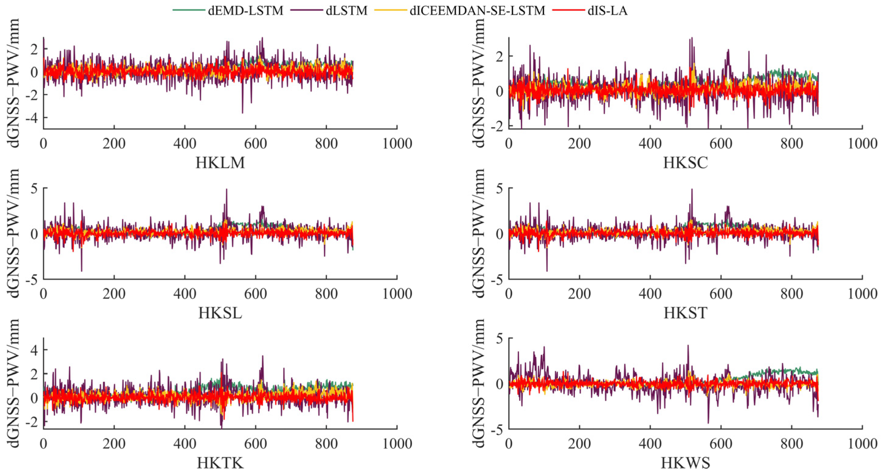
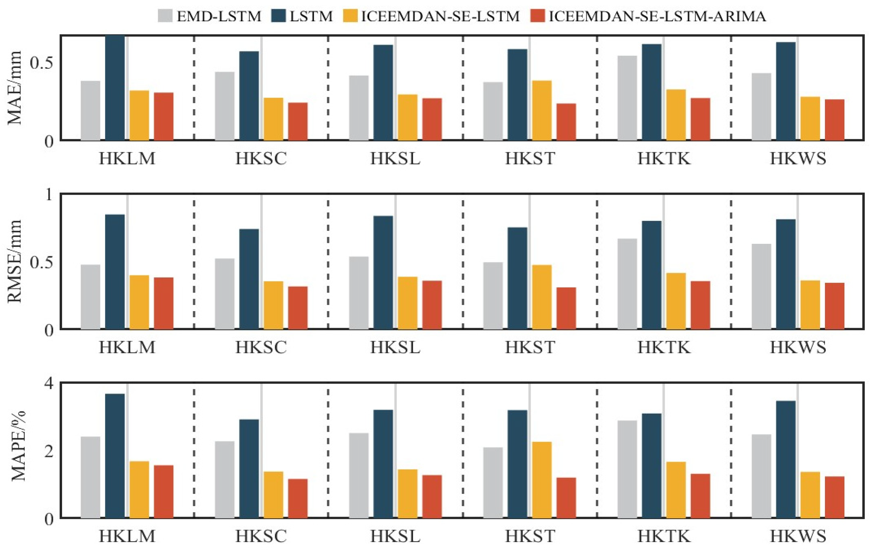
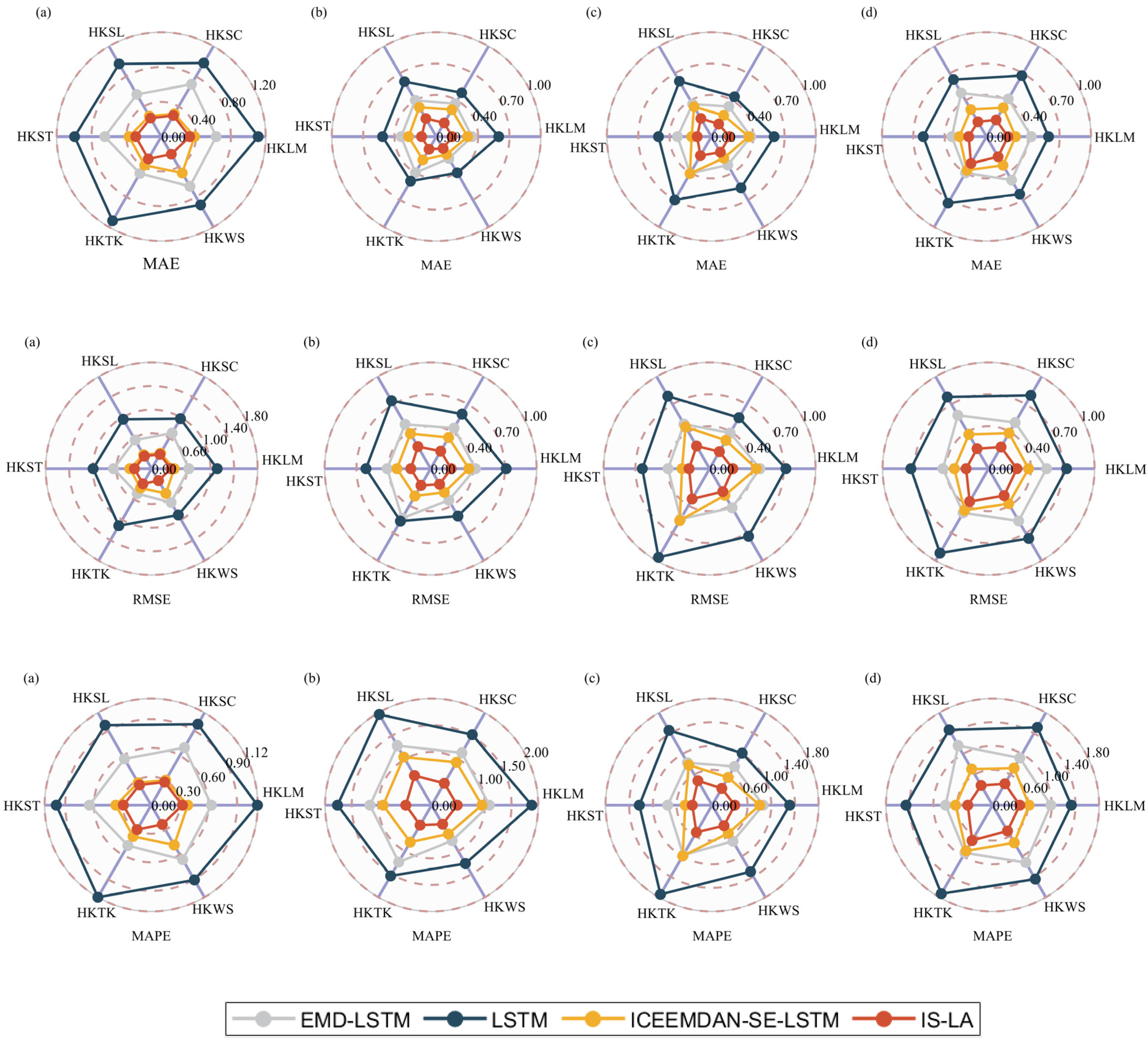
4.1. GNSS-PWV Forecasts for Different Sites

This experiment aims to verify the universality and spatial stability of the IS-LA model under the influence of geographic heterogeneity through multi-site comparative analysis. The comparison experiments at six sites can systematically test whether the model has the ability to predict water vapor across regions and environments, and if it can avoid overfitting or local optimization problems due to the specificity of the data at a single site. For the GNSS-PWV data of the six sites, the first 90% of the GNSS-PWV data with 1 h resolution at each site in 2022 is selected as the training set for the initial training of the model, and the last 10% is used as the test set for evaluating the final performance of the model. Firstly, the GNSS-PWV data are decomposed using the ICEEMDAN method and the white noise standard deviation (0.15) is chosen from a range of 0.05–0.25 to balance modal aliasing suppression and signal fidelity. Values below 0.15 preserved pseudo-modalities while values above 0.25 over-smoothed fluctuations: a value of 0.15 maximized the preservation of multiscale features. The maximum number of iterations (50) and noise addition (200) is performed to ensure convergence of the decomposition. Taking the HKLM site as an example, the decomposition process of ICEEMDAN generates a large number of patterns, and the decomposition results of the HKLM site are given in the graph in Figure 4.
As shown in Figure 4, the ICEEMDAN method generates an 11th-order pattern. As the order increases, the fluctuations in the decomposed components become progressively smaller, resulting in a change pattern that is more intuitive compared to the original PWV data. This allows the overall trend to become more apparent. The initial high-frequency components exhibit a disordered state, capturing the detailed feature information of the original sequence and highlighting the complex changes in the data over a short period. In contrast, the middle components display some regularity, enabling a more accurate representation of the significant fluctuations in the original PWV. Finally, the last components reflect the overall changes in the GNSS-PWV for Hong Kong in 2022.
The self-similarity of the components is analyzed using the sample entropy as an index and the IMF components with similar sample entropy values are merged. The embedding dimension (m = 2) follows the time-series convention for phase space reconstruction. The similarity tolerance R of 0.2 times the standard deviation of the original PWV sequence is empirically calibrated. According to Figure 5, it can be seen that the sample entropy values of IMF1 and IMF2 subsequences are higher than 1, indicating high complexity and sequence volatility, so these two types of sequences are merged as high-frequency components and IMF3~IMF8 components with values between 1 and 0.01 are merged into low-frequency components, Components close to 0 are incorporated into trend components. The sample entropy values for the HKLM site are shown in Figure 5 below.
The residuals of each model with the original values of different sites are shown in Figure 6. The IS-LA model outperforms the other models in predicting PWV, which is mainly manifested in smaller and more concentrated residuals. Notably, the IS-LA model outperforms the others in predicting PWV. This is primarily evidenced by smaller and more centralized residuals, leading to higher prediction accuracy. The substantial prediction errors associated with the combined EMD sequence decomposition algorithm are mainly due to severe modal aliasing within the frequency components derived from decomposing the PWV sequence. When predicted individually, increasing the number of decomposed components results in error accumulation, ultimately producing excessive prediction errors. Additionally, the ICEEMDAN-SE-LSTM model does not adequately separate random noise from the various elements within the linear or nonlinear trends of the PWV data, which may negatively impact its prediction results. In contrast, the ICEEMDAN algorithm employed in our model effectively suppresses modal aliasing and allows for the extraction of distinct feature components from the PWV sequence. Therefore, the reconstructed components are then predicted separately using both linear and nonlinear models, leading to improved accuracy compared to the ICEEMDAN-SE-LSTM model.
Figure 7 presents the statistics of three different accuracy metrics for six stations. The improvement in PWV prediction accuracy with our constructed IS-LA model varies across the stations; however, it consistently outperforms the other three models at all locations. This result indicates that the IS-LA model has superior generalization ability and robustness. In addition, as can be seen in Figure 7, there is a small improvement in the prediction accuracy of the model constructed in this paper compared to the ICEEMDAN-SE-LSTM model, which employs the same decomposition and reconstruction strategy but uses only a single neural network model for prediction, and the difference in performance can be attributed to the different characteristics of the models. For the low-frequency and trend components, ARIMA shows an advantage due to its ability to accurately capture linear patterns, whereas LSTM has limitations in handling linear patterns compared to ARIMA. Our analysis suggests that ARIMA’s strengths in modeling linear trends and seasonal patterns, in combination with the other components in the IS-LA model, help to close the performance gap. The IS-LA model leverages the strengths of both ARIMA and LSTM by assigning the different types of components to the most appropriate models, thereby improving the overall prediction accuracy.
From Table 2, it can be concluded that the average prediction results of the four models at the six stations show good prediction accuracy. In particular, the accuracy of the IS-LA hybrid model demonstrates significant enhancement compared to the traditional LSTM neural network prediction model. Specifically, the MAE is reduced by 56.81%, the RMSE is decreased by 56.78%, and the MAPE is lowered by 60.34%. Compared to the EMD-LSTM prediction model, which utilizes the EMD decomposition strategy and a single neural network for item-by-item prediction, our proposed model achieves significant improvements: the average MAE, the average RMSE, and the average MAPE are reduced by 38.41%, 37.91%, and 47.08%, respectively. Additionally, when compared to the ICEEMDAN-SE-LSTM prediction model, which also employs a single neural network with the same decomposition and reconstruction strategy, our model shows a reduction of 15.16% in the average MAE, a 13.58% reduction in the average RMSE, and an 11.91% decrease in the average MAPE. Overall, the IS-LA hybrid model demonstrates the best performance and highest stability in predicting results across different states.

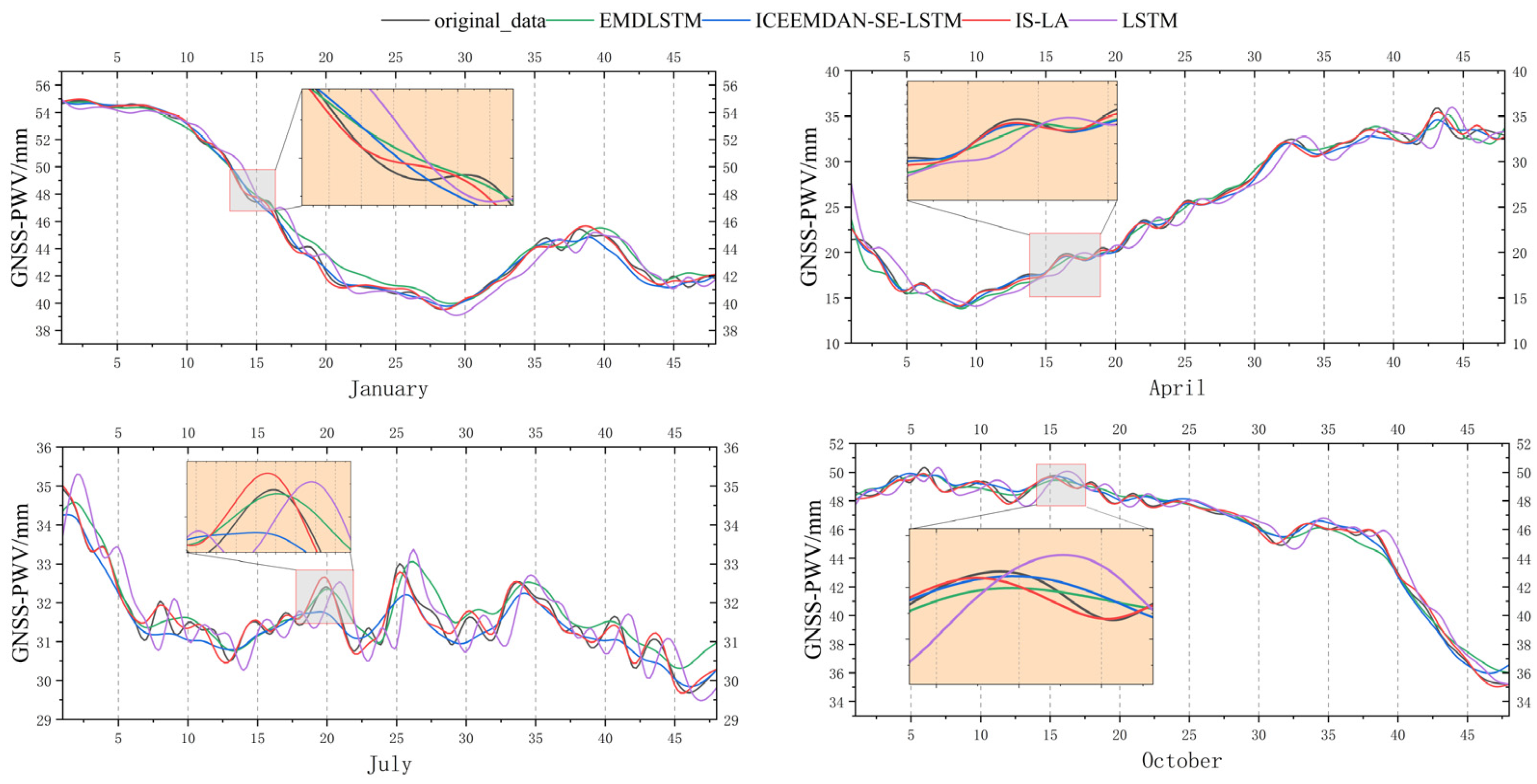
4.2. GNSS-PWV Forecasts for Different Months

Typical months of different seasons are selected for comparative analysis in this experiment, aiming to verify the generalization ability and seasonal adaptability of the IS-LA model under variable meteorological conditions. Considering the large sea level fluctuations of GNSS-PWV, the cross-seasonal comparison experiment can test whether the model can accurately capture the nonlinear patterns of water vapor changes under different climatic backgrounds and avoid the risk of the model losing its generalizability due to over-adaptation to a single season. In this section, we use the mid-season months (January, April, July, and October) of HKLM stations as the experiments, which can not only avoid the interference of sudden changes in meteorological elements during the seasonal transition period, but also obtain seasonally typical and stable data samples so as to systematically evaluate the prediction accuracy of the model under four typical climate scenarios, namely spring, summer, autumn, and winter, and provide a multidimensional performance validation of the model for practical application. In this experiment, the GNSS-PWV data of the first 29 days of each mid-season month are selected as the training set, the GNSS-PWV data of the last 48 h of each month are used as the test set, and the predictions of different models are shown in Figure 8.
Figure 8 shows the GNSS-PWV results for four months. It is clear that the red solid line representing the IS-LA model predictions follows closely the black line representing the original sequence. It is worth noting that the GNSS-PWV variations in January, April, and October are relatively smooth. In contrast, July has the most volatile GNSS-PWV. This drastic fluctuation is mainly due to the high sea surface temperature around Hong Kong during the summer months of July. The high specific heat capacity of seawater causes a large amount of water vapor to evaporate into the atmosphere in summer, which affects the fluctuation of GNSS-PWV [33]. In addition, as Hong Kong is a densely populated city, the urban heat island effect increases the local air temperature, which further enhances the convective activities and promotes the accumulation and release of GNSS-PWV. The specific accuracy metrics of different models are shown in Table 3.
Table 3 presents the prediction index of PWV at the HKLM site over four months. The prediction accuracy of the IS-LA model shows a descending order of performance for July, October, January, and April. The RMSE ranges from 0.19 mm to 0.43 mm, while the MAE ranges from 0.15 mm to 0.33 mm. When PWV experiences significant fluctuations in July, complex meteorological factors cause the linear and nonlinear components to interact. The IS-LA model effectively separates the prediction of these two components, resulting in a better performance with an RMSE of 0.22 mm. January is a transitional month in terms of climate, characterized by frequent shifts between warm, humid air and cold air. These fluctuations complicate water vapor transport and atmospheric circulation. Additionally, January features various precipitation patterns, with localized strong convection and rainfall events leading to an irregular distribution of water vapor. This complexity increases the uncertainty of model predictions. Although all comparison models exhibited lower prediction accuracy in January, the IS-LA model still outperforms them by achieving a maximum RMSE of 0.43 mm.
Scientific and reliable performance evaluation is a crucial prerequisite for models in real prediction applications. In order to visualize the differences between models in different months and different stations, radargrams are plotted as shown in Figure 9 to compare the MAE, RMSE, and MAPE values of different models in GNSS-PWV predictions at different stations. Specifically, each axis in the plot represents a station, and the length of the axis represents the size of the accuracy index. Due to seasonal factors, there are large prediction differences among the models at different stations. One reason for this phenomenon may be that the stations HKTK, HKSL, HKSC, and HKLM are located at the seashore and their tropospheric delays are affected by the interaction between oceanic water vapor and the complex boundary layer. The complex vertical distribution of water vapor leads to difficulty in estimating the GNSS-PWV, which makes the average prediction accuracies of the four months lower than those of the four months that are mainly dependent on the inland stations of HKST and HKWS as these mainly rely on local evaporation and atmospheric circulation to transport water vapor and have a relatively simple vertical distribution of water vapor. Overall, the model has a good prediction performance with high accuracy in predicting the GNSS-PWV of most of the stations in Hong Kong for the four different months. This indicates that the IS-LA model has some regional applicability and shows stability in the application in Hong Kong.

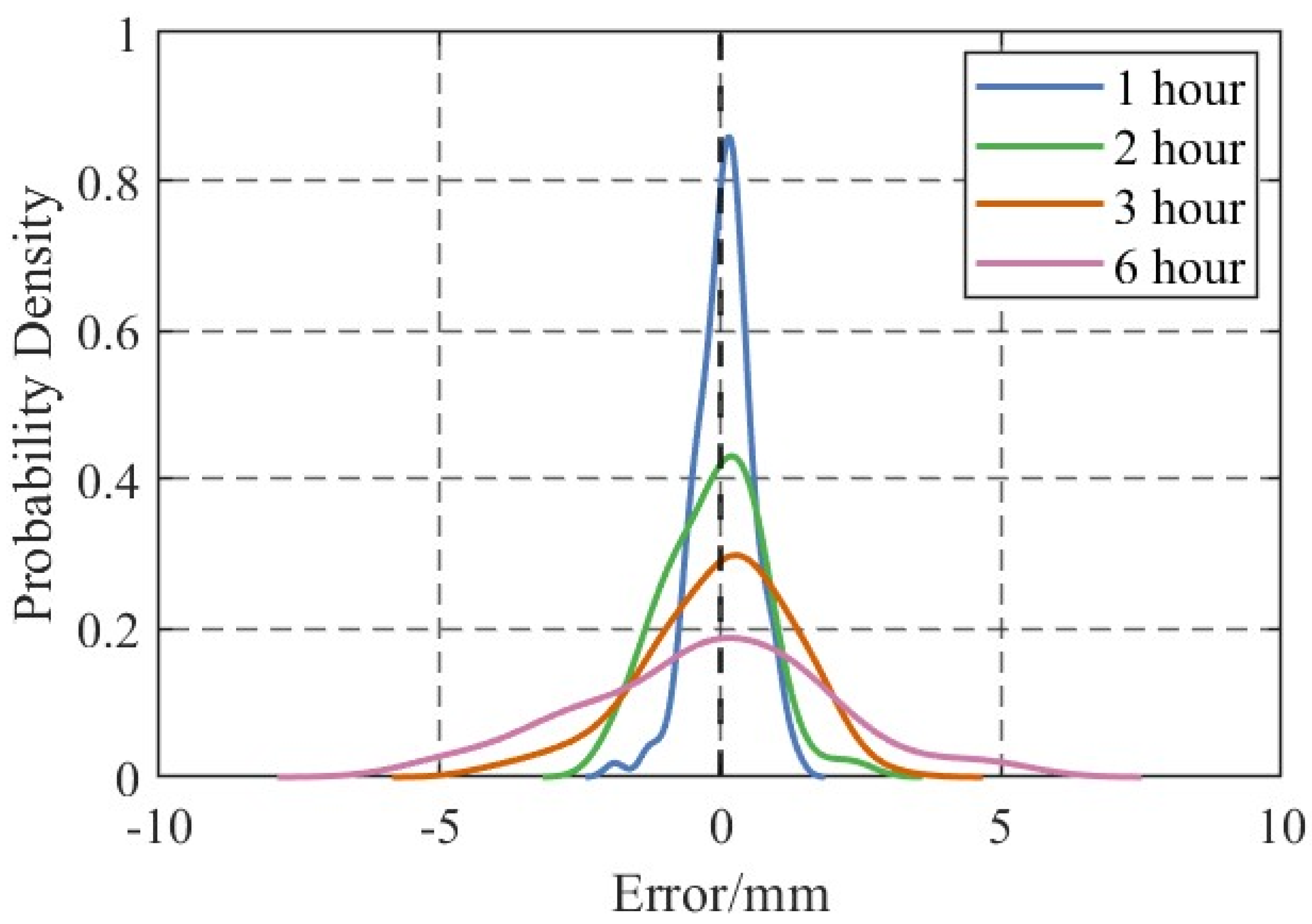
4.3. GNSS-PWV Forecasts for Different Steps

The advantages of the proposed IS-LA hybrid model for the single-step prediction of GNSS-PWV data have been demonstrated in the previous subsections. While predicting a single unknown value is straightforward, multi-step prediction—where multiple unknown values are predicted simultaneously based on their temporal relationships—presents more significant challenges and holds more promising applications. In this section, we conduct experiments with varying prediction intervals of 1 h, 2 h, 3 h, and 6 h. We utilize hourly GNSS-PWV data from six stations in Hong Kong, collected from December 1 to December 31, totaling 744 data points. The time step size is set to 24 while all other parameters remain constant, allowing us to examine the impact of different prediction intervals on the performance of the proposed model. The accuracy for the six stations at various prediction step sizes during December is presented in Table 4.
The results indicate that the six stations’ RMSE, MAE, and MAPE gradually increase as the prediction step increases. In December, for a prediction step of 1 h, the RMSE for the stations ranged from 0.45 to 0.53 mm, with an average of 0.51 mm. The MAE ranged from 0.37 to 0.42 mm, with an average of 0.40 mm, while the MAPE varied from 1.75% to 1.91%, with an average of 1.85%. When the prediction step was extended to 6 h, the RMSE increased to a range of 2.12 to 2.25 mm, with a mean of 2.19 mm. The MAE increased to between 1.64 and 1.80 mm, averaging 1.73 mm, and the MAPE rose to between 7.53% and 8.37%, with an average of 7.74%.
Figure 10 shows the standardized distribution of the errors of the IS-LA hybrid model when four different step sizes are used on the December test set of Hong Kong waters. It is obvious from the figure that as the prediction step size increases, the peak of the error distribution gradually decreases and the range of the distribution becomes wider. Specifically, the error distribution curve of 1 h prediction has the highest peak value and the error is highly concentrated near the 0 value, indicating that the model has the smallest error in short-time prediction and optimal stability and accuracy. Furthermore, with the extension of the prediction step lengths to 2, 3, and 6 h, the peak value of the error distribution decreases significantly and the distribution interval widens continuously. This trend suggests that the uncertainty of the measurement error increases with the extension of the prediction step. In conclusion, the IS-LA hybrid model shows high reliability and accuracy in predicting GNSS-PWV at 3 h steps. However, when the prediction time was extended to 6 h, the accuracy of the model decreased, although it still provided reasonably feasible predictions.

5. Discussion

Accurate prediction of GNSS-PWV is of great significance for improving GNSS positioning accuracy, meteorological monitoring, and climate research. The IS-LA hybrid model proposed in this paper demonstrates superior prediction performance in different stations at different months, and in multi-step prediction effectively solves the pseudo-modal and residual noise problems in the traditional decomposition methods, improves the physical fidelity of the signal decomposition, and reduces the number of modeling times and computational complexity. The model innovatively integrates ICEEMDAN decomposition and SE and LSTM-ARIMA parallel prediction framework, providing a new and effective method for GNSS-PWV prediction. Moreover, it promotes the development of the application of GNSS technology in multiple fields such as meteorology, oceanography, and environment. Future research can further optimize the model parameter settings, introduce more external factors and data sources to enrich the model input information, and explore the combination of more advanced deep learning architectures and algorithms with the existing model frameworks to further enhance the model’s modeling and forecasting capabilities for complex time series data as well as to expand the application of GNSS-PWV forecasting techniques in practical scenarios such as drought monitoring and extreme weather forecasting.

6. Conclusions

In this paper, we validate the accuracy of GNSS-PWV in Hong Kong and provide a comprehensive analysis of its characteristics. We propose a hybrid prediction model called IS-LA, which integrates the ICEEMDAN decomposition method and sample entropy along with a parallel-driven prediction module that consists of a data-driven LSTM and a model-driven ARIMA functional model. To efficiently extract the potential multidimensional features of GNSS-PWV sequences, we utilize the ICEEMDAN decomposition algorithm. This method significantly reduces the uncertainty associated with the complexity of the original data series. It addresses the issues related to pseudo-patterns and residual noise commonly generated by the CEEMDAN method. This creates optimal conditions for an in-depth examination of the internal characteristics of the time series. We reconstruct multiple components into high-frequency, low-frequency, and trend terms to optimize the balance between prediction accuracy and model efficiency. This strategy decreases the training time required for the model and minimizes the cumulative errors that may occur from making predictions item-by-item after decomposition. Following the results of static and nonlinear tests on the reconstructed components, we selected the most appropriate and scientifically validated prediction model. This ultimately led to a more accurate hybrid prediction model for GNSS-PWV in Hong Kong.
We analyzed the correlation between the GNSS-PWV data obtained using GAMIT10.71 software and the Radio-PWV data derived from sounding measurements. The correlation coefficient exceeded 0.95 and the RMSE was less than 3.10 mm, indicating that the prediction data are high quality. To assess the stability of our model, we conducted GNSS-PWV prediction experiments at various sites. The results of our quantitative analysis demonstrated that our algorithm significantly reduced the average RMSE, average MAE, and average MAPE metrics. Compared to the LSTM, EMD-LSTM, and ICEEMDAM-SE-LSTM models, our algorithm reduced average RMSE by 56.78%, 37.91%, and 13.58%, respectively, across different sites. In the experiments predicting GNSS-PWV across different months while accounting for seasonal variations, the RMSEs of our IS-LA model were as follows: January—0.43 mm, April—0.19 mm, July—0.22 mm, and October—0.27 mm. Overall, the IS-LA model developed in this study demonstrates higher prediction accuracy than other models. Our findings also revealed that the IS-LA model maintains high reliability and accuracy when predicting GNSS-PWV within 3 h. However, extending the prediction time to 6 h significantly decreases accuracy, although the model still delivers usable prediction outcomes. Specifically, the six stations’ RMSE, MAE, and MAPE increased as the prediction step lengthened. For instance, the RMSE for the June stations with a 1 h prediction step ranged from 0.45 mm to 0.53 mm, averaging 0.51 mm. In contrast, when the prediction step was extended to 6 h, the RMSE rose to between 2.12 mm and 2.25 mm, with an average of 2.19 mm. These results suggest that while the IS-LA model shows promise for short-term forecasting, further optimization is needed to enhance its performance for medium- and long-term predictions.
Overall, we demonstrate that the IS-LA model is highly accurate and efficient for predicting GNSS-PWV. It effectively predicts GNSS-PWV in the complex climatic environment of the Hong Kong region and can provide accurate predictions of the PWV for different months and various training durations. This capability is significant for advancing research in GNSS meteorology. We plan to incorporate external factors into the modeling system and establish a multivariate input prediction mechanism for future work. This approach aims to enhance the interpretability of the results while maintaining a focus on prediction accuracy. Additionally, we will fuse PWV derived from multi-system GNSS with other multi-source PWV. By expanding our experiments to include more stations, we aim to improve the model’s applicability and provide robust data support for further meteorological research.

Author Contributions

Conceptualization, X.L. and J.Z. (Jie Zhao); methodology, J.Z. (Jie Zhao), Z.Y. and Y.X.; software, J.Z. (Jie Zhao); validation, J.Z. (Jie Zhao), X.C. and N.D.; formal analysis, J.Z. (Jie Zhao); investigation, J.Z. (Jie Zhao) and C.Y.; resources, J.Z. (Jie Zhao) and C.Y.; data curation, J.Z. (Jie Zhao) and J.Z. (Jun Zhao); writing—original draft preparation, J.Z. (Jie Zhao); writing—review and editing, J.Z. (Jie Zhao), N.D. and X.C.; visualization, J.Z. (Jie Zhao); supervision, J.Z. (Jie Zhao) and C.Y.; project administration, L.Z.; funding acquisition, J.Z. (Jie Zhao). All authors have read and agreed to the published version of the manuscript.

Funding

This research was funded by the National Natural Fund of China grants (grant number 42271461), the Natural Science Foundation of Sichuan Province (grant numbers 2024NSFSC0070) and the State Key Laboratory of Geohazard Prevention and Geoenvironment Protection Independent Research Project (SKLGP2021Z022).

Data Availability Statement

RINEX data for IGS stations were provided by the IGS Data Centre at Wuhan University (gnsswhu.cn, accessed on 1 April 2024). RINEX data for the Hong Kong CORSs were provided by the Geodetic Services Department of Hong Kong (geodetic.gov.hk, accessed on 1 April 2024). The sounding station observations were provided by the University of Wyoming, USA (http://weather.uwyo.edu/upperair/, accessed on accessed on 20 April 2024). We thank the Hong Kong Geodetic Service and the University of Wyoming for providing relevant data and products, and the Department of Earth Atmospheric and Planetary Sciences of the Massachusetts Institute of Technology for providing the GAMIT/GLOBK10.71 software.

Acknowledgments

The authors would like to thank the reviewers for their careful reading of our paper and for their valuable suggestions for revision which have improved its presentation.

Conflicts of Interest

The authors declare no conflicts of interest.

Abbreviations

The following abbreviations are used in this manuscript:
PWVPrecipitable Water Vapor
GNSSGlobal Navigation Satellite System
CORSsContinuously Operating Reference Stations
EMDEmpirical Mode Decomposition
CEEMDANComplete Ensemble Empirical Mode Decomposition with Adaptive Noise
ICEEMDANImproved Complete Ensemble Empirical Mode Decomposition with Adaptive Noise
SESample Entropy
LSTMLong Short-Term Memory
ARIMAAutoregressive Integrated Moving Average model
MAEMean Absolute Error
RMSERoot Mean Square Error
MAPEMean Absolute Percentage Error
ZTDZenith Tropospheric delay
ZHDZenith Hydrostatic Delay
ZWDZenith Wet Delay
IMFIntrinsic Mode Function
AICAkaike Information Criterion
BICBayesian Information Criterion
ADFAugmented Dickey–Fuller Test
BDSBinary Decision Diagrams Test

Appendix A. Appendix Information and Missing Data Rates for Seven Sites in the Hong Kong Region

In this study, the Hong Kong region (22°9′N to 22°37′N, 113°52′E to 114°30′E) was selected as the test area for predicting GNSS-PWV. We selected six CORSs and one sounding station in the area which are in different directions and have a low data missing rate. However, there are still a few missing data in the solved GNSS-PWV and Radio-PWV time series due to receiver failures or poor observing conditions, and the station information and missing data rates are shown in the following table. In this paper, we use cubic spline interpolation with a sliding window of 72 h to interpolate the small amount of missing data.
Table A1. Information and data missing rate of selected sites in Hong Kong region.
StationsLatitudeLongitudeElevation (m)Missing Data Rates
HKLM22.219114.12011.2450.27%
HKSC22.322114.14123.1190.27%
HKSL22.372113.93899.2640.27%
HKST22.395114.184261.5340.58%
HKTK22.547114.22325.4620.82%
HKWS22.434114.33566.1070.58%
Radio22.310114.17066.0000.19%

References

  1. Liu, Z.; Fan, Q.; Lv, Q.; Wang, M.; Wu, J.; Liu, Y.; Xu, C. A Novel Linear Rainfall Forecast Model Based on GNSS Observations and CAPE. IEEE Trans. Geosci. Remote Sens. 2024, 62, 1–9. [Google Scholar] [CrossRef]
  2. Zhao, Q.; Ma, X.; Yao, W.; Liu, Y.; Yao, Y. A Drought Monitoring Method Based on Precipitable Water Vapor and Precipitation. J. Clim. 2020, 33, 10727–10741. [Google Scholar] [CrossRef]
  3. Zhao, Q.; Yao, Y.; Yao, W. GPS-based PWV for precipitation forecasting and its application to a typhoon event. J. Atmos. Sol.-Terr. Phys. 2018, 167, 124–133. [Google Scholar] [CrossRef]
  4. Wu, Z.; Lu, C.; Han, X.; Zheng, Y.; Wang, B.; Wang, J.; Liu, Y.; Liu, Y. Real-time shipborne multi-GNSS atmospheric water vapor retrieval over the South China Sea. GPS Solut. 2023, 27, 179. [Google Scholar] [CrossRef]
  5. Jiang, P.; Liu, R.; Huo, Y.; Wu, Y.; Ye, S.; Wang, S.; Mu, X.; Zhu, L. Retrieving the Atmospheric Water Vapor Profile Combining FY-4A/GIIRS and Ground-Based GNSS PWV in Hong Kong Region. IEEE Trans. Geosci. Remote Sens. 2024, 63, 1–9. [Google Scholar] [CrossRef]
  6. He, Q.; Zhang, K.; Wu, S.; Zhao, Q.; Wang, X.; Shen, Z.; Li, L.; Wan, M.; Liu, X. Real-Time GNSS-Derived PWV for Typhoon Characterizations: A Case Study for Super Typhoon Mangkhut in Hong Kong. Remote Sens. 2020, 12, 104. [Google Scholar] [CrossRef]
  7. Lian, D.; He, Q.; Li, L.; Fu, E.; Zhang, K. Accuracy Assessment of ERA5-ZTD/PWV and Response of Typhoon Events in China. J. Catastrophology 2024, 39, 23–28. [Google Scholar]
  8. Li, H.B.; Wang, X.M.; Wu, S.Q.; Zhang, K.F.; Chen, X.L.; Qiu, C.; Zhang, S.T.; Zhang, J.L.; Xie, M.Q.; Li, L. Development of an Improved Model for Prediction of Short-Term Heavy Precipitation Based on GNSS-Derived PWV. Remote Sens. 2020, 12, 4101. [Google Scholar] [CrossRef]
  9. Yan, X.; Yang, W.; Gao, M.; Ding, N.; Zhang, W.; Li, L.; Hou, Y.; Zhang, K. The WOA-CNN-LSTM-Attention Model for Predicting GNSS Water Vapor. IEEE Trans. Geosci. Remote Sens. 2024, 62, 1–15. [Google Scholar] [CrossRef]
  10. Sharifi, M.A.; Souri, A.H. A hybrid LS-HE and LS-SVM model to predict time series of precipitable water vapor derived from GPS measurements. Arab. J. Geosci. 2015, 8, 7257–7272. [Google Scholar] [CrossRef]
  11. Ghaffari-Razin, S.R.; Majd, R.D.; Hooshangi, N. Regional modeling and forecasting of precipitable water vapor using least square support vector regression. Adv. Space Res. 2023, 71, 4725–4738. [Google Scholar] [CrossRef]
  12. Acheampong, A.; Obeng, K. Application of GNSS derived precipitable water vapour prediction in West Africa. J. Geod. Sci. 2019, 9, 41–47. [Google Scholar] [CrossRef]
  13. Ghaffari Razin, M.-R.; Voosoghi, B. Modeling of precipitable water vapor from GPS observations using machine learning and tomography methods. Adv. Space Res. 2022, 69, 2671–2681. [Google Scholar] [CrossRef]
  14. Du, Z.; Yao, Y.; Zhang, B.; Zhao, Q. Precipitable water vapor estimation from Himawari-8/AHI observations using a stacking machine learning model. Atmos. Res. 2024, 301, 107281. [Google Scholar] [CrossRef]
  15. Yue, Y.; Ye, T. Predicting precipitable water vapor by using ANN from GPS ZTD data at Antarctic Zhongshan Station. J. Atmos. Sol.-Terr. Phys. 2019, 191, 105059. [Google Scholar] [CrossRef]
  16. Senkal, O.; Yildiz, B.Y.; Sahin, M.; Pestemalci, V. Precipitable water modelling using artificial neural network in Cukurova region. Environ. Monit. Assess. 2012, 184, 141–147. [Google Scholar] [CrossRef]
  17. Ghaffari-Razin, S.R.; Davari Majd, R.; Hooshangi, N. Estimation of precipitable water vapor (PWV) using generalized regression neural network (GRNN) and comparison against tomography, ECMWF, Saastamoinen, GPT3 and ANN models. J. Water Health 2023, 49, 243–264. [Google Scholar] [CrossRef]
  18. Jain, M.; Manandhar, S.; Lee, Y.H.; Winkler, S.; Dev, S. Forecasting Precipitable Water Vapor Using LSTMs. In Proceedings of the IEEE AP-S Symposium on Antennas and Propagation and CNC/USNC-URSI Joint Meeting, Montréal, QC, Canada, 5–10 July 2020. [Google Scholar]
  19. Huang, Y.; Wei, G.; Ren, R. Improved BP neural network model for prediction of atmospheric precipitable water vapor. J. Navig. Position. 2020, 8, 63–67, 110. [Google Scholar]
  20. Kou, M.; Zhang, K.; Zhang, W.; Ma, J.; Ren, J.; Wang, G. Application research of combined model based on VMD and MOHHO in precipitable water vapor Prediction. Atmos. Res. 2023, 292, 106841. [Google Scholar] [CrossRef]
  21. Liu, Y.P.; Wang, Y.; Wang, Z. RBF Prediction Model Based on EMD for Forecasting GPS Precipitable Water Vapor and Annual Precipitation. Adv. Mater. Res. 2013, 765–767, 2830–2834. [Google Scholar] [CrossRef]
  22. Shangguan, M.; Dang, M.; Yue, Y.; Zou, R. A Combined Model to Predict GNSS Precipitable Water Vapor Based on Deep Learning. IEEE J. Sel. Top. Appl. Earth Obs. Remote Sens. 2023, 16, 4713–4723. [Google Scholar] [CrossRef]
  23. Yuan, Z.D.; Lin, X.; Xu, Y.S.; Dai, R.T.; Yang, C.; Zhao, L.W.; Han, Y.K. The VMD-Informer-BiLSTM-EAA Hybrid Model for Predicting Zenith Tropospheric Delay. Remote Sens. 2025, 17, 672. [Google Scholar] [CrossRef]
  24. Wu, J.; Wu, L.; Sun, M.; Lu, Y.N.; Han, Y.H. Application of Boundary Local Feature Scale Adaptive Matching Extension EMD Endpoint Effect Suppression Method in Blasting Seismic Wave Signal Processing. Shock Vib. 2021, 2021, 2804539. [Google Scholar] [CrossRef]
  25. Yang, H.; Liu, S.; Zhang, H. Adaptive estimation of VMD modes number based on cross correlation coefficient. J. Vibroengineering 2017, 19, 1185–1196. [Google Scholar] [CrossRef]
  26. Ren, Y.; Suganthan, P.N.; Srikanth, N. A Comparative Study of Empirical Mode Decomposition-Based Short-Term Wind Speed Forecasting Methods. IEEE Trans. Sustain. Energy 2015, 6, 236–244. [Google Scholar] [CrossRef]
  27. Liang, Y.; Lin, Y.; Lu, Q. Forecasting gold price using a novel hybrid model with ICEEMDAN and LSTM-CNN-CBAM. Expert Syst. Appl. 2022, 206, 117847. [Google Scholar] [CrossRef]
  28. Kou, M.; Zhang, W.; Ren, J.; Zhang, X. A combined model based on data decomposition and multi-model weighted optimization for precipitable water vapor forecasting. Earth Sci. Inform. 2022, 15, 2213–2230. [Google Scholar] [CrossRef]
  29. Xiao, X.; Lv, W.; Han, Y.; Lu, F.; Liu, J. Prediction of CORS Water Vapor Values Based on the CEEMDAN and ARIMA-LSTM Combination Model. Atmosphere 2022, 13, 1453. [Google Scholar] [CrossRef]
  30. Bevis, M.; Businger, S.; Herring, T.A.; Rocken, C.; Anthes, R.A.; Ware, R.H. GPS Meteorology: Remote Sensing of Atmospheric Water Vapor Using the Global Positioning System. J. Geophys. Res. Atmos. 1992, 97, 15787–15801. [Google Scholar] [CrossRef]
  31. Colominas, M.A.; Schlotthauer, G.; Torres, M.E. Improved complete ensemble EMD: A suitable tool for biomedical signal processing. Biomed. Signal Process. Control 2014, 14, 19–29. [Google Scholar] [CrossRef]
  32. Graves, A.; Schmidhuber, J. Framewise phoneme classification with bidirectional LSTM and other neural network architectures. Neural Netw. 2005, 18, 602–610. [Google Scholar] [CrossRef] [PubMed]
  33. He, Q.M.; Shen, Z.; Wan, M.F.; Li, L.J. Precipitable Water Vapor Converted from GNSS-ZTD and ERA5 Datasets for the Monitoring of Tropical Cyclones. IEEE Access 2020, 8, 87275–87290. [Google Scholar] [CrossRef]
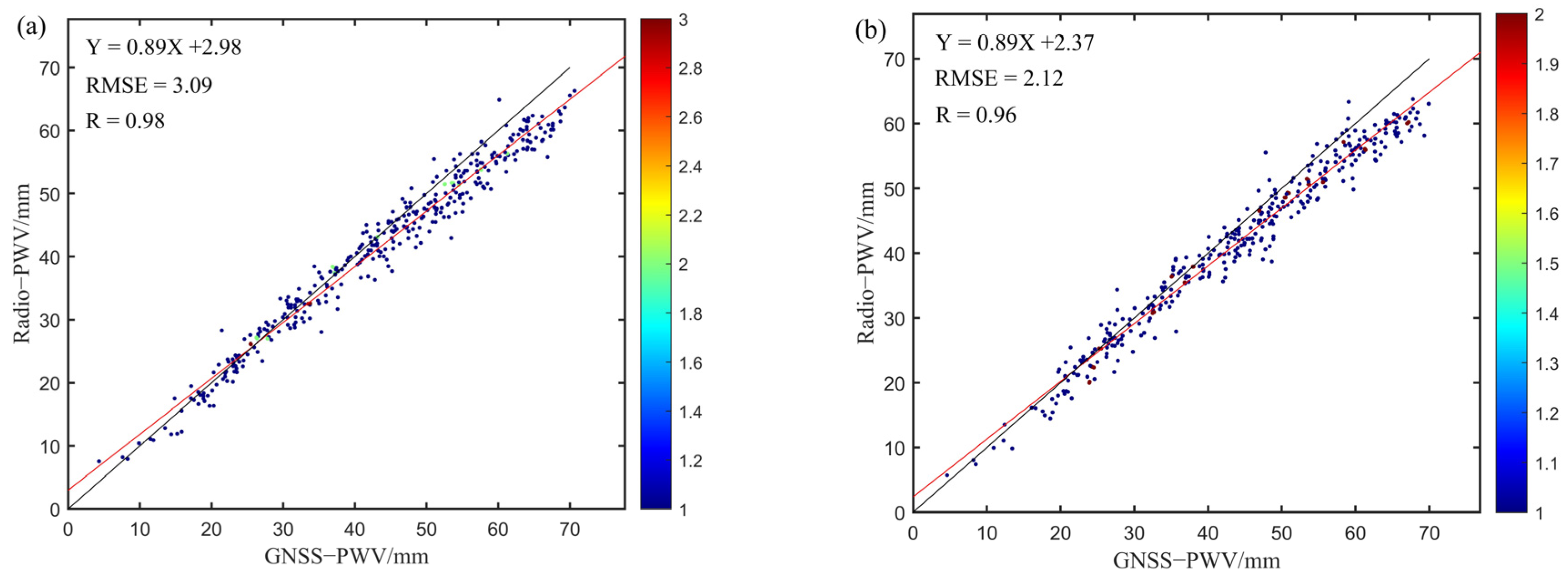
Figure 1. Distribution of sites.
Remotesensing 17 01675 g001
Figure 2. Correlation analysis of GNSS-PWV and Radio-PWV corresponding moments. (a) GNSS-PWV correlation with sounding PWV at moment 12 in 2022; (b) GNSS-PWV correlation with sounding PWV at moment 0 in 2022.
Remotesensing 17 01675 g002
Figure 3. IS-LA hybrid model flowchart.
Remotesensing 17 01675 g003
Figure 4. HKLM site PWV decomposition chart.
Remotesensing 17 01675 g004
Figure 5. SE values for the IMF component of the HKLM site.
Remotesensing 17 01675 g005
Figure 6. Residual plots for different models at each site.
Remotesensing 17 01675 g006
Figure 7. Three accuracy metrics for different models in six stations.
Remotesensing 17 01675 g007
Figure 8. Projected effect charts for different months.
Remotesensing 17 01675 g008
Figure 9. Radar charts of the model’s predictive indicators (a) for January; (b) for April; (c) for July; and (d) for October.
Remotesensing 17 01675 g009
Figure 10. Plot of normal distribution of errors for different prediction steps.
Remotesensing 17 01675 g010
Table 1. Comparison of GNSS-PWV and Radio-PWV accuracy at HKSC stations.
TimeBIAS/mmRMSE/mm
MaximumMinimumAverage
12 moments11.05−6.861.983.09
0 moment11.21−7.701.162.12
Table 2. Average accuracy metrics for different models.
ModelsMean-MAE/mmMean-RMSE/mmMean-MAPE/%
LSTM0.610.803.25%
EMD-LSTM0.430.552.43%
ICEEMDAN-SE-LSTM0.310.401.46%
IS-LA0.260.341.29%
Table 3. HKLM site prediction indicators for different months.
ModelsJanuaryAprilJulyOctober
MAERMSEMAPEMAERMSEMAPEMAERMSEMAPEMAERMSEMAPE
LSTM1.111.524.83%0.600.711.88%0.600.721.31%0.590.741.33%
EMD-LSTM0.630.842.72%0.340.421.08%0.380.480.86%0.430.550.98%
ICEEMDAN-SE-LSTM0.380.501.53%0.300.360.94%0.330.440.80%0.280.380.62%
IS-LA0.330.431.37%0.150.190.48%0.170.220.38%0.210.270.46%
Table 4. IS-LA hybrid modeling using different prediction step accuracy metrics.
Predicted StepsMean-MAE/mmMean-RMSE/mmMean-MAPE/%
1 h0.400.511.85%
2 h0.770.983.67%
3 h0.921.164.31%
6 h1.732.197.74%
Disclaimer/Publisher’s Note: The statements, opinions and data contained in all publications are solely those of the individual author(s) and contributor(s) and not of MDPI and/or the editor(s). MDPI and/or the editor(s) disclaim responsibility for any injury to people or property resulting from any ideas, methods, instructions or products referred to in the content.

