Using Geodetic Data to Monitor Hydrological Drought at Different Spatial Scales: A Case Study of Brazil and the Amazon Basin

Abstract

Geodetic data, especially from the Global Navigation Satellite System (GNSS) and Gravity Recovery and Climate Experiment (GRACE)/GRACE Follow-On (GFO), are extensively employed in hydrological drought monitoring across various spatial scales due to their unique spatial resolution. In recent years, Brazil has experienced some of the most severe drought events in decades. This study focuses on Brazil and its northeastern Amazon Plain, investigates the spatiotemporal characteristics of terrestrial water storage (TWS) changes, and calculates the hydrological drought severity index (DSI) and meteorological drought index for comprehensive analysis of drought conditions. The results indicate that the time series of TWS changes derived from different data sources are highly correlated, with correlation coefficients exceeding 0.85, and are consistent with the trend of precipitation variation, reflecting notable seasonal fluctuations, i.e., an increase in precipitation during the spring and summer seasons leads to a rise in TWS, while a decrease in precipitation during the autumn and winter seasons triggers a reduction in TWS. In terms of spatial distribution, the annual amplitude of TWS variation is most pronounced in the northeastern Amazon Plain. The highest amplitude, approximately 800 mm, is observed near the Amazon River Basin, and this amplitude gradually weakens from northeast to southwest. GNSS and GRACE/GFO data reveal four hydrological drought events in Brazil from 2013 to 2024, with two of these events detected using GRACE/GFO data. The most severe droughts occurred between 2023 and 2024, primarily driven by prolonged precipitation deficits and the El Niño phenomenon, lasting up to nine months. Additionally, three distinct drought events were identified in the Amazon Plain, suggesting that its hydrological dynamics significantly influenced Brazil’s drought conditions. These results demonstrate the capability of geodetic data to effectively monitor water deficit and drought duration on both small spatial scales and short timeframes, thereby providing crucial support for timely responses to and the management of hydrological drought events.

1. Introduction

In the context of global warming, droughts have become more frequent and severe in many regions, leading to substantial economic and social losses [1,2]. Consequently, it is imperative to enhance our understanding of current drought and flood risks by comprehensively analyzing their spatiotemporal characteristics. Researchers typically classify drought into several essential types: meteorological drought, soil drought, hydrological drought, vegetation drought, socioeconomic drought, and ecological drought [3]. Among them, the formation mechanism of hydrological drought is particularly complex. It is not only affected by atmospheric conditions but also involves the processes of moisture transport within the atmosphere, which significantly impact both precipitation accumulation and runoff changes. Hydrological drought, characterized by its gradual onset and complexity, can persist even after precipitation and other related factors return to normal [4,5].

Numerous studies have shown that terrestrial water storage (TWS) changes are closely related to hydrological drought events [2,6,7]. TWS encompasses surface water and groundwater [8], and its fluctuations reflect the supply and demand of water resources, with long-term declines typically signaling the onset of drought. By monitoring TWS changes, researchers can effectively predict the occurrence and severity of droughts, as decreases in TWS are commonly associated with reduced precipitation, increased evaporation, and declining groundwater levels. Integrating TWS changes with hydrological drought models can help improve early warning capabilities and subsequently support the development of scientific drought response strategies.

TWS changes lead to some extent to alterations in the Earth’s gravity field, a phenomenon that the Gravity Recovery and Climate Experiment (GRACE) satellite and its successor GRACE Follow-On (GFO) effectively monitor. Additionally, Global Navigation Satellite System (GNSS) stations deployed on the Earth’s surface can detect surface deformations resulting from dynamic fluctuations in water storage. As space geodesy technologies continue to advance, they have substantially accelerated the development of hydrogeodesy. Notably, the quantification of TWS changes using GRACE/GFO data, alongside the inversion of TWS through GNSS-derived hydrological load displacement, has emerged as a prominent research focus for the study of surface mass changes and hydrological drought events [9], providing a critical scientific basis for global hydrological drought assessment and water resource management.

At large spatial scales, researchers primarily employ GRACE/GFO to quantify TWS changes [10,11,12], and it has been widely applied in monitoring hydrological drought [13,14]. However, since GRACE and GFO occur after nearly a one-year gap and the spatial resolution of GRACE/GFO remains between 300 and 500 km, these limitations constrain the ability of GRACE/GFO to monitor TWS changes in small-scale regions over short time scales. In contrast, in regions with relatively dense GNSS station distribution, hydrological loading displacements derived from GNSS have been demonstrated to effectively monitor daily TWS changes at small scales with a spatial resolution of 50–100 km, and it has been widely applied in various regions worldwide, including California [15,16,17], Washington and Oregon [18], Australia [19,20], Southwest China [21,22,23], and the Yellow River Basin in China [3,24]. Two primary methods exist for the GNSS inversion of regional TWS changes: one is Green’s function method based on the spatial domain [15,25,26], and the other is the Slepian basis function method based on the frequency domain [19]. Jiang et al. (2021) [27] calculated the drought severity index (DSI) using GNSS-TWS to assess drought conditions in Yunnan, China. Since then, GNSS-DSI has been increasingly used as a hydrological drought index to monitor drought conditions worldwide [28,29,30,31].

Brazil’s diverse terrain and climate are exemplified by the Amazon Plain (AMP), which encompasses the Amazon Basin in the north and accounts for about one-third of the country’s total area. In the past decade, Brazil has suffered several drought events due to extreme changes in precipitation and the recurring occurrence of El Niño [5,28]. Therefore, this study focuses on Brazil, with particular emphasis on northern Brazil (including the Amazon Basin), and employs geodetic techniques to investigate the spatiotemporal characteristics of TWS changes at different spatial scales and quantify their drought conditions. The details are as follows: (a) Inversion of daily and monthly TWS changes using GRACE/GFO data and GNSS vertical displacement time series and comparison with the results obtained from meteorological and hydrological data to identify the spatiotemporal patterns of TWS changes in Brazil; (b) Quantification of drought events in Brazil between August 2013 and August 2024 by integrating the drought severity index (GRACE-DSI and GNSS-DSI) calculated from geodetic data with the meteorological drought indices (SPI and SPEI); (c) Spatiotemporal analysis of TWS changes at small spatial scales in the AMP as an example and to explore the advantages and disadvantages of geodesy techniques for inverting TWS changes at different spatial scales. The results demonstrate that geodetic techniques effectively monitor regional TWS changes and drought events at large and small spatial scales.

2. Study Area and Datasets

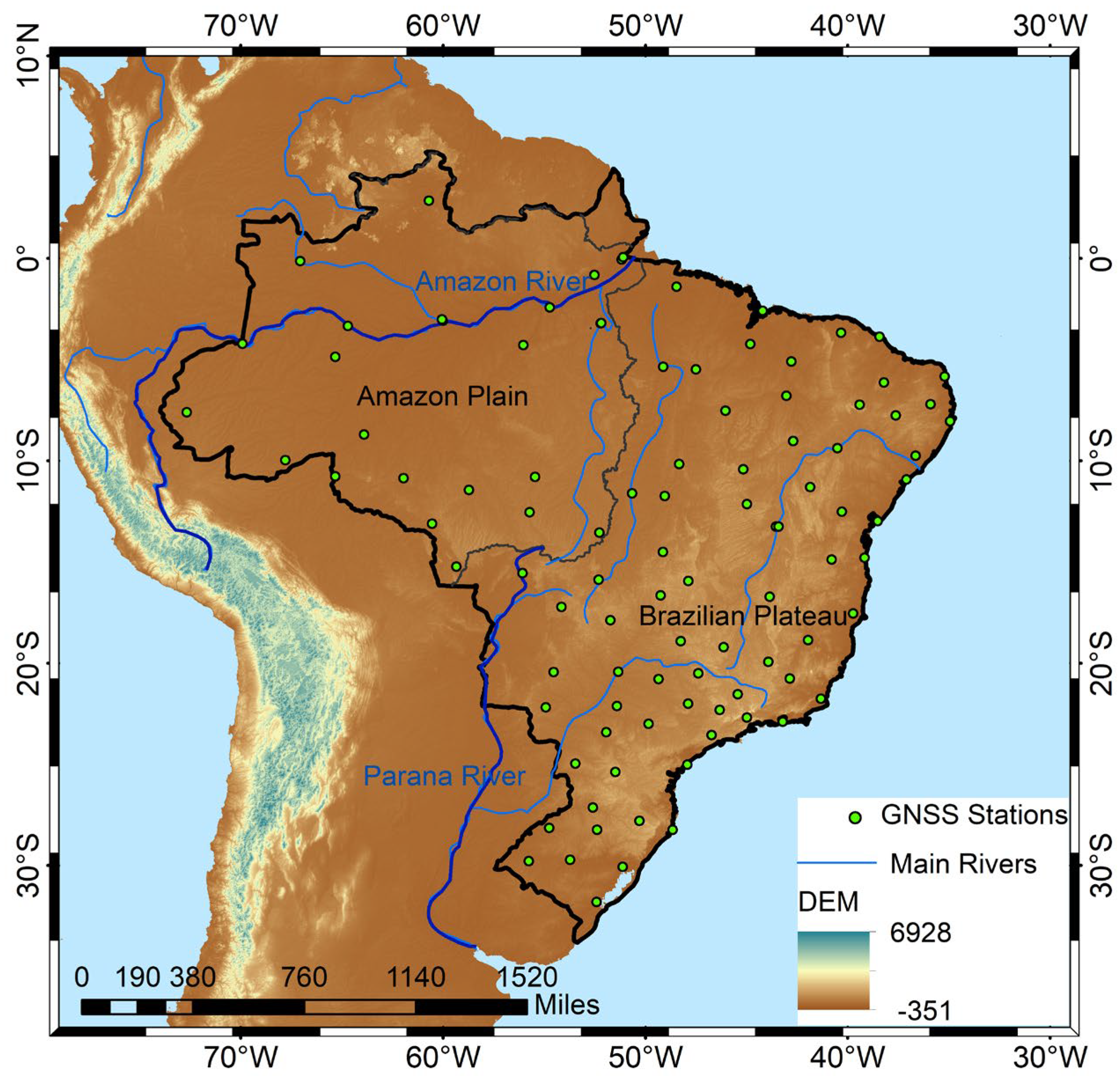
2.1. Study Area

Brazil is in the eastern part of South America and covers an area of about 8.5 million square kilometers. It has distinct north–south topography features, with the Brazilian Plateau in the center–south and the AMP (including the Amazon Basin) predominating in the north. Notably, the AMP accounts for about one-third of Brazil’s total area, making it the most extensive plain in the world. Most parts of Brazil belong to the tropics, with a diverse climate characterized by tropical rainforests in the north, savannahs in the center, and a subtropical monsoon humid climate in the south, and is susceptible to the effects of climatic anomalies. In particular, the AMP in northern Brazil has experienced frequent droughts over the past decade, some due to extreme weather events (e.g., sudden declines in precipitation and rising temperatures) and others owing to the El Niño phenomenon [5,11,32]. In July 2024, the Brazilian government reportedly issued an announcement stating that the region is facing the most severe drought in recent years, which has persisted for 12 months. Given these ongoing challenges, it is crucial to quantify and comprehensively analyze the region’s drought duration.

2.2. GNSS Data

This study adopts vertical displacement time series data from 81 GNSS stations in Brazil from 1 August 2013 to 31 August 2024 provided by the Nevada Geodetic Laboratory (NGL) at the University of Nevada, USA (http://geodesy.unr.edu/, accessed on 1 October 2024). These selected station data were processed using GipsyX-1.0 software and the latest Repro 3.0 product from NASA’s Jet Propulsion Laboratory [33]. Figure 1 illustrates the distribution of these GNSS stations in Brazil, with an average distance of about 350 km.

To obtain GNSS data related to hydrological loads, this study conducted preprocessing work on GNSS stations by applying the non-tidal atmospheric load (NTAL) and non-tidal ocean load (NTOL) models in the geometric center reference framework provided by the German Research Centre for Geosciences (GFZ) (http://esmdata.gfz-potsdam.de:8080/repository, accessed on 1 October 2024) to deduct the effects of atmospheric and oceanic loads [34]. The annual amplitude of crustal deformation induced by NTAL ranges from 0.77 to 1.67 mm (Figure S1), and that caused by NTOL is between 0.02 and 0.49 mm (Figure S2). Subsequently, this study utilized the least squares fitting method to obtain the GNSS vertical displacement time series dominated by seasonal hydrological signals. Finally, the GNSS vertical displacements were complemented using the Kriging Kalman filter method to obtain continuous TWS changes for subsequent inversion [35]. Figure S3 displays the time series of four stations before and after preprocessing.

2.3. GRACE/GFO Data

This study utilized the GRACE/GFO RL0603 version of the Mascon model released by the Centre for Space Research (CSR) at the University of Texas (https://www2.csr.utexas.edu/, accessed on 1 October 2024) to infer TWS changes. The CSR Mascon product is derived from GRACE’s second-order spherical harmonic coefficients and does not rely on any prior information other than the spherical harmonic coefficients. The processing of this product includes C20 replacement, first-order term correction, and Glacial Isostatic Adjustment (GIA) correction. Additionally, for GFO products, the C30 coefficient is also replaced [36]. Cubic spline interpolation was used to fill the missing data within the GRACE mission period. This study did not address the nearly one-year data gap between the GRACE and GFO missions.

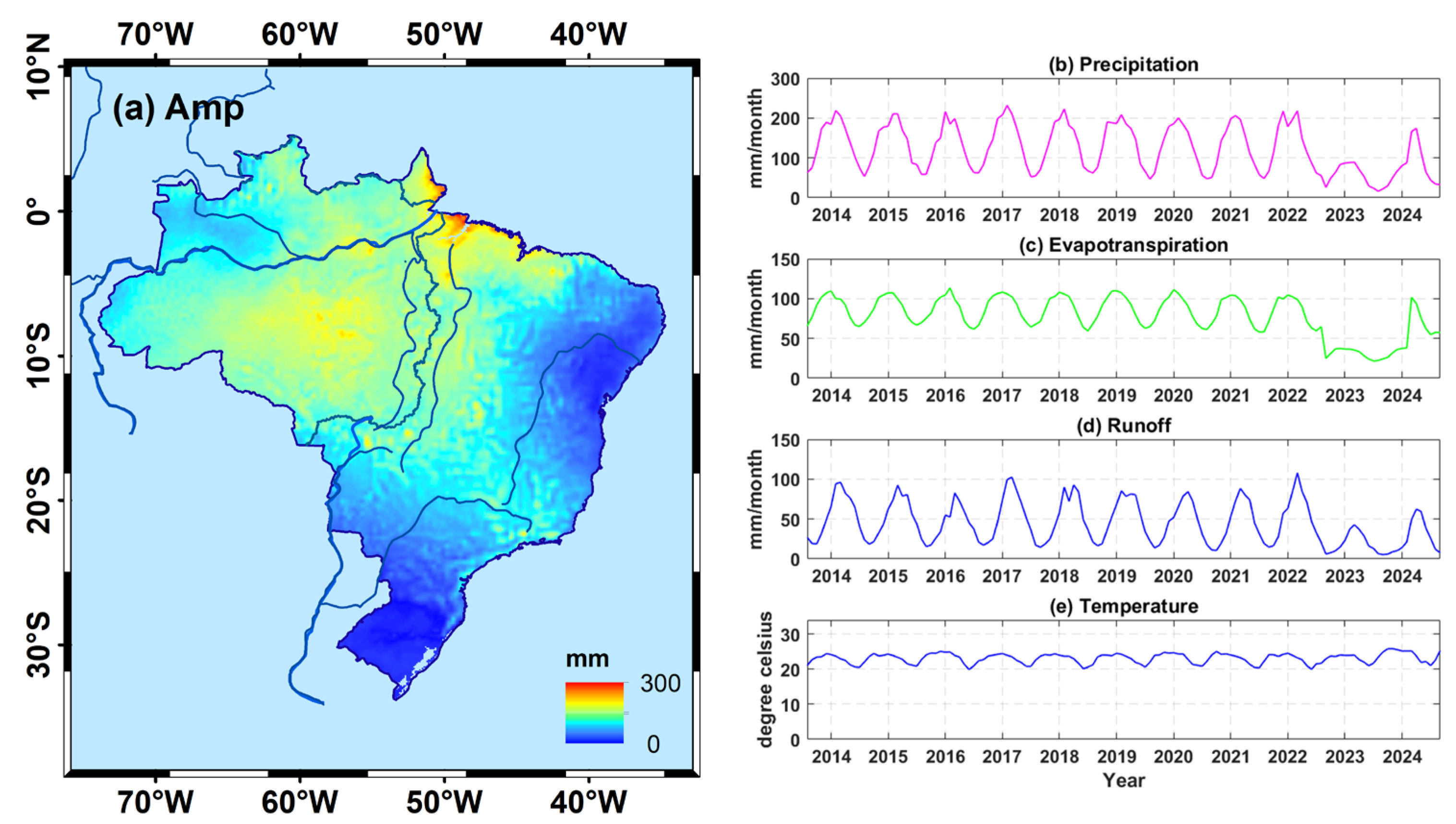
2.4. Hydrometeorological Data

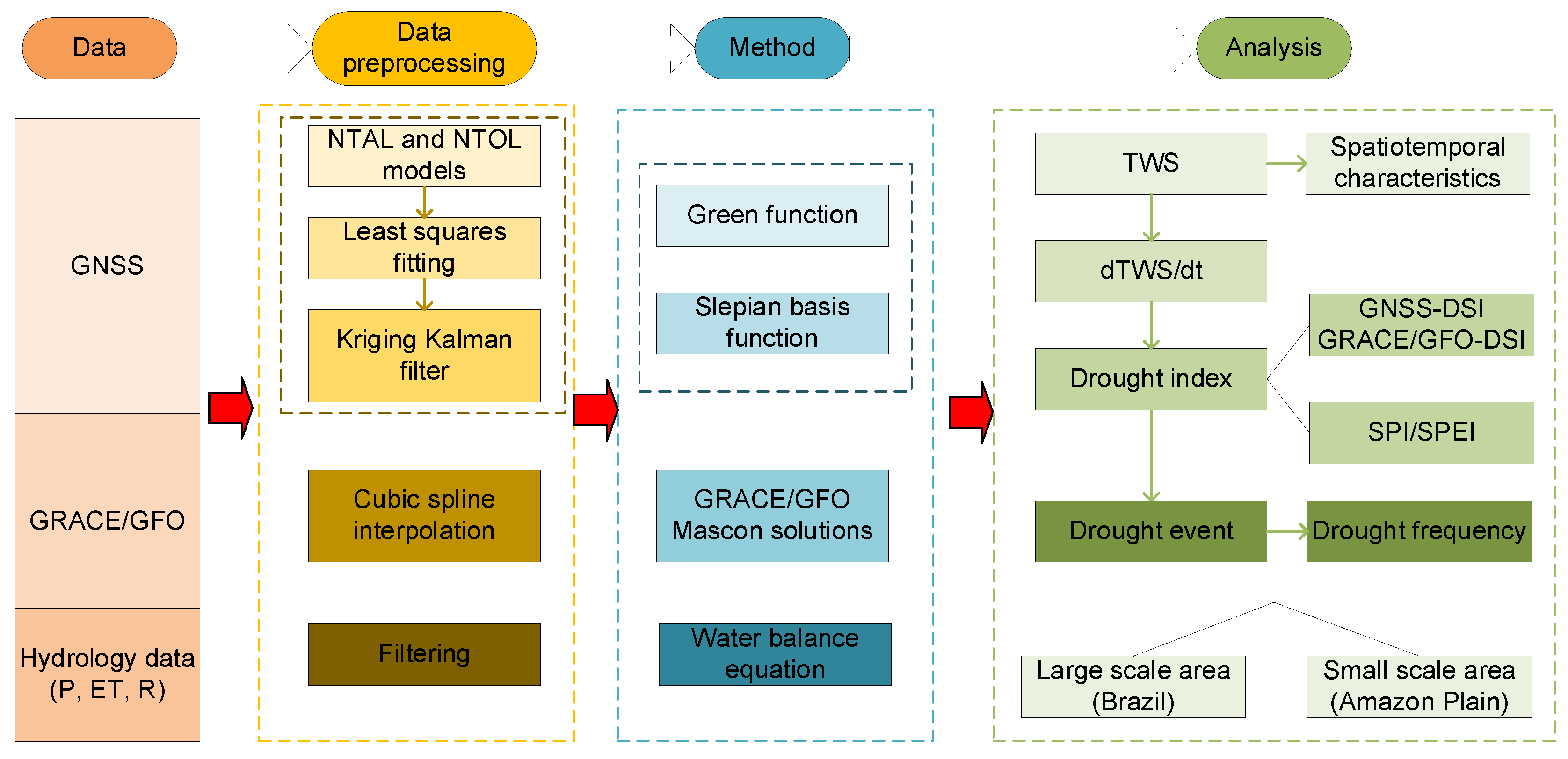
This study employs ERA5-Land data [37] provided by the European Centre for Medium-Range Weather Forecasts (ECMWF) to analyze meteorological drought events based on the water balance equation using precipitation (P), evapotranspiration (ET), runoff (R), and 2 m temperature data. The spatial resolution of these data was 0.1° × 0.1°, and the temporal resolution was in monthly intervals (https://cds.climate.copernicus.eu/, accessed on 1 November 2024). Figure 2a displays the annual amplitude of precipitation data, divided into two parts by the boundary of the AMP, with a significantly higher precipitation variation in the northeastern AMP than in the southwestern Brazilian Plateau. Figure 2b–e presents the time series of meteorological and hydrological data. The results exhibit clear seasonality, with peaks occurring each year’s summer months. Notably, P, ET, and R sharply declined in the second half of 2022. Additionally, Brazil has experienced a gradual increase in overall temperature due to global warming.

For a specific regional scale, TWS changes can be expressed by the water balance equation [38], and the calculation formula is as follows:

$$dTWS/dt=P-ET-R$$

(1)

The TWS derivatives calculated from meteorological and hydrological data reflect changes in the middle of each month. In contrast, the TWS derivatives derived from geodetic data represent changes at the beginning or end of a month. To standardize the temporal resolution, the study filters the P-ET-R data [39] for consistency across the datasets.

$$\widehat{F}(t)={\displaystyle \frac{1}{4}}F(t-1)+{\displaystyle \frac{1}{2}}F(t)+{\displaystyle \frac{1}{4}}F(t+1)$$

(2)

where $F$ denotes P, ET, and R, and $\widehat{F}$ denotes the corresponding filtered data.

3. Methodology

3.1. Green’s Function Method

Since changes in mass load within the Earth lead to crustal deformation, which can be monitored by GNSS stations placed on the surface, we can establish a mathematical linear relationship between mass load changes and surface deformation using Green’s function method within the framework of mass load theory, as outlined by Farrell (1972) [25]:

$$u=Gx+e$$

(3)

where $x$ represents the mass load vector in the form of equivalent water height (EWH); $u$ represents the GNSS vertical displacement deformation vector; $G$ denotes the Green’s function in the study area; and $e$ represents the error terms.

This study estimates the EWH value of the grid at an interval of 1° and adopts the least squares model proposed by Argus et al. (2014) to invert the TWS change in the regional grid as follows [15]:

$${\left(\left(Gx-u\right)/\sigma \right)}^2+{\beta }^2{\left(L\left(x\right)\right)}^2\to \min$$

(4)

$$E={\sigma }^2$$

(5)

where $\sigma$ denotes the standard deviation, and $L$ represents the Laplace operator. Due to the fact that the number of GNSS stations is less than the number of regional grids, it is necessary to add the Laplace operator as a spatial smoothing constraint in the inversion model. $\beta$ denotes the regularization factor, determined by the generalized cross-validation (GCV) method, with a value of 0.042 (Figure S4). Therefore, the formula for calculating the EWH value of each grid is as follows.

$${\widehat{x}}_1={\left({G^T}_1{E}^{-1}{G}_1+\beta L^{T}L\right)}^{-1}{G^T}_1{E}^{-1}{d}_1$$

(6)

In order to compare the results with those obtained from GRACE/GFO and meteorological and hydrological data at the same scale, this study resampled the daily TWS changes into monthly changes and differentiated the results over time to obtain the TWS changes, as in the following equation:

$$dTWS/dt=TWS\left(t+1\right)-TWS\left(t\right)$$

(7)

3.2. Slepian Basis Function Method

Green’s function method inverts TWS changes from a spatial domain perspective. In contrast, the Slepian basis function method proposed by Han and Razeghi (2017) applies the load Love number to estimate the mass load in the study area from a frequency domain perspective [19], and then the EWH corresponding to the mass load in the study area can be expressed as follows:

$${\sigma }_L\left(\theta ,\lambda ,t\right)=a{\displaystyle \sum _{\beta =1}^J{\gamma }_{\beta }{s}_{\beta }^{EWH}\left(t\right)g_{\beta }\left(\theta ,\lambda \right)}$$

(8)

where $a$ is the radius of the earth; $J$ is the truncation order; ${\gamma }_{\beta }$ denotes the eigenvalue; $s_{\beta }^{EWH}$ is the coefficient of Slepian basis function; $g_{\beta }$ is the Slepian basis function.

This study sets the Slepian basis function parameters with a maximum order of 40, a buffer extension of 2°, a Gaussian filter of 400 km and adopts the first 42 basis functions with concentration ratios greater than 0.4 (Figures S5 and S6), and then computes the basis function coefficients by inverting 81 GNSS stations.

3.3. Drought Index

SPI and SPEI are commonly used to study meteorological drought characteristics, so this study uses these two as meteorological drought indices. They both originate from the same standardization process based on probability, with differences in the input variables and fitting functions [28,30]. For SPEI, this study exploits a three-parameter log-logistic probability density function (PDF) to fit the input data and estimates the potential evapotranspiration (PET) using the Thornthwaite method:

$$\left\{\begin{array}{c}{D}_s^i=P_m^i-PE{T}_m^i\\ G\left(y_s^i\right)={\displaystyle {\int }_{-\infty }^{y}g\left(D_s^i\right)dt}\\ SPE{I}_s^i={\Phi }^{-1}\left(G\left(y_s^i\right)\right)\end{array}\right.$$

(9)

where $P$ is the precipitation, and $D$ is the difference between $P$ and $PET$. g is the log-logistic function, and $G$ denotes the cumulative distribution function (CDF).

An appropriate fitting function is crucial for the calculation of SPI. Since the precipitation distribution is non-normal, several PDFs (especially Gamma PDF and Pearson III PDF) have been applied to fit the input variables in previous studies. This study chose SPI based on Pearson Type III because it is more consistent with SPEI:

$$\left\{\begin{array}{c}F\left(x_s^i\right)={\displaystyle {\int }_{-\infty }^{x}f\left(t_s^i\right)dt}\\ SP{I}_s^i={\Phi }^{-1}\left(F\left(x_s^i\right)\right)\end{array}\right.$$

(10)

where $t_s^i$ represents precipitation data at the s-th epoch with the i-month time scale. $f$ is Pearson III PDF, and $F$ is the corresponding CDF.

For the hydrological drought index, this study calculated GRACE-DSI and GNSS-DSI based on daily and monthly TWS changes. Jiang et al. (2021) [27] developed DSI based on GRACE-DSI [14], and the mathematical formula is as follows:

$$DS{I}_{i,j}={\displaystyle \frac{TW{S}_{i,j}-\overline{TW{S}_j}}{{\sigma }_j}}$$

(11)

where $TW{S}_{i,j}$ represents the TWS in the j-th month of the i-th year; $\overline{TW{S}_j}$ denotes the average of the j-th month of each year; x represents the standard deviation.

Figure 3 shows the research flowchart of this study.

4. Results

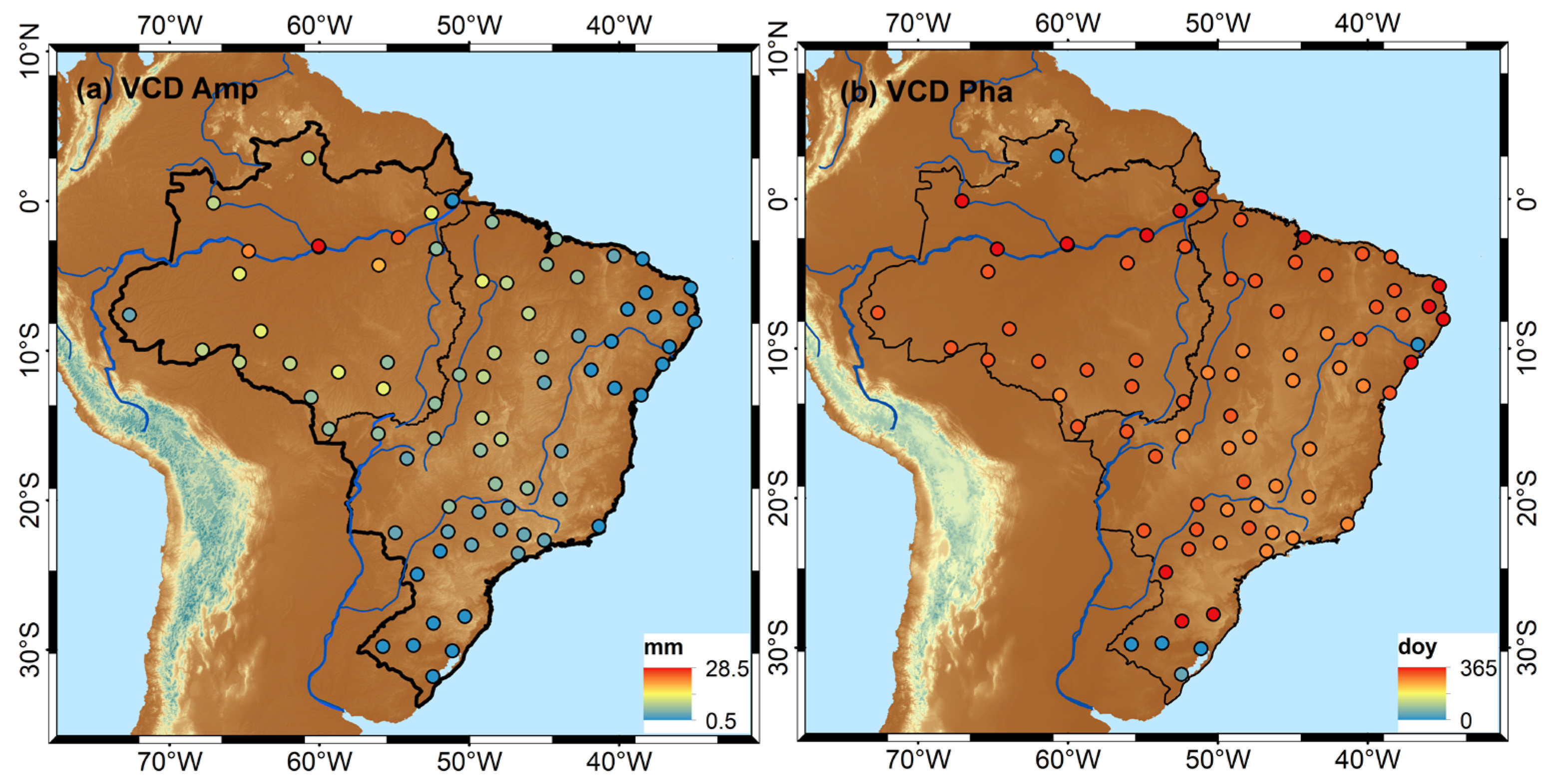
4.1. Spatiotemporal Characteristics of GNSS-Derived Hydrological Mass Loading

This study employs the PCA method to decompose the GNSS vertical displacement time series to investigate better the GNSS vertical displacements induced by hydrological load. Figure 4 illustrates the spatial variations and temporal functions of the five principal components (PCs) derived from the PCA, with the first five PCs explaining 84.7% of the variance in the filtered data. PC1 and PC2 together explain 83.5% of the variance, with PC1 accounting for 70%, revealing the spatiotemporal characteristics of hydrological load in Brazil. From the spatial function, the hydrological load at the GNSS stations in the AMP exhibits substantial variations, with almost all GNSS stations showing positive contributions, and the seasonal variation is most pronounced in northern Brazil, gradually decreasing toward the southwest. In terms of time function, surface subsidence due to increased hydrological load predominantly occurs in spring and summer, whereas surface uplift primarily takes place in autumn and winter as precipitation gradually decreases (Figure 2b). PC2 captures the primary variation pattern of hydrological load, highlighting local and secondary variation features beyond the long-term trend represented by PC1. The variance explained by PC3, PC4, and PC5 accounts for only 16.5%, and these three principal components reflect changes in data detail and complex local signals, including short-term crustal movements, specific seasonal variations, or noise patterns [32].

This study also investigates the annual variation of GNSS vertical displacements (see Figure 5a). The results indicate that the annual amplitude of GNSS vertical displacements in Brazil gradually decreases from north to south, which is consistent with the PC1’s spatial pattern. This further demonstrates that PC1’s spatial and temporal function predominantly reveals the spatiotemporal characteristics of hydrological loads in Brazil. The NAUS station near the Amazon River exhibits the most significant annual amplitude, up to 28 mm, the same as the results of previous studies [28]. Other GNSS stations in the AMP show annual amplitudes of more than 6 mm, mostly between 10 and 20 mm, and overall larger than in southern Brazil (1 to 13 mm). The results suggest that the displacement load at stations near major rivers, such as the Amazon Basin, undergoes substantial changes, while stations far away from the main rivers, e.g., in southeastern Brazil, experience weaker displacement loads.

This study also estimates the annual phase, defined as the point when GNSS vertical displacement reaches its lowest level, to determine the time that maximizes the seasonality of TWS changes. As shown in Figure 5b, the annual phase of GNSS vertical displacement mostly occurs between 260 and 290 days.

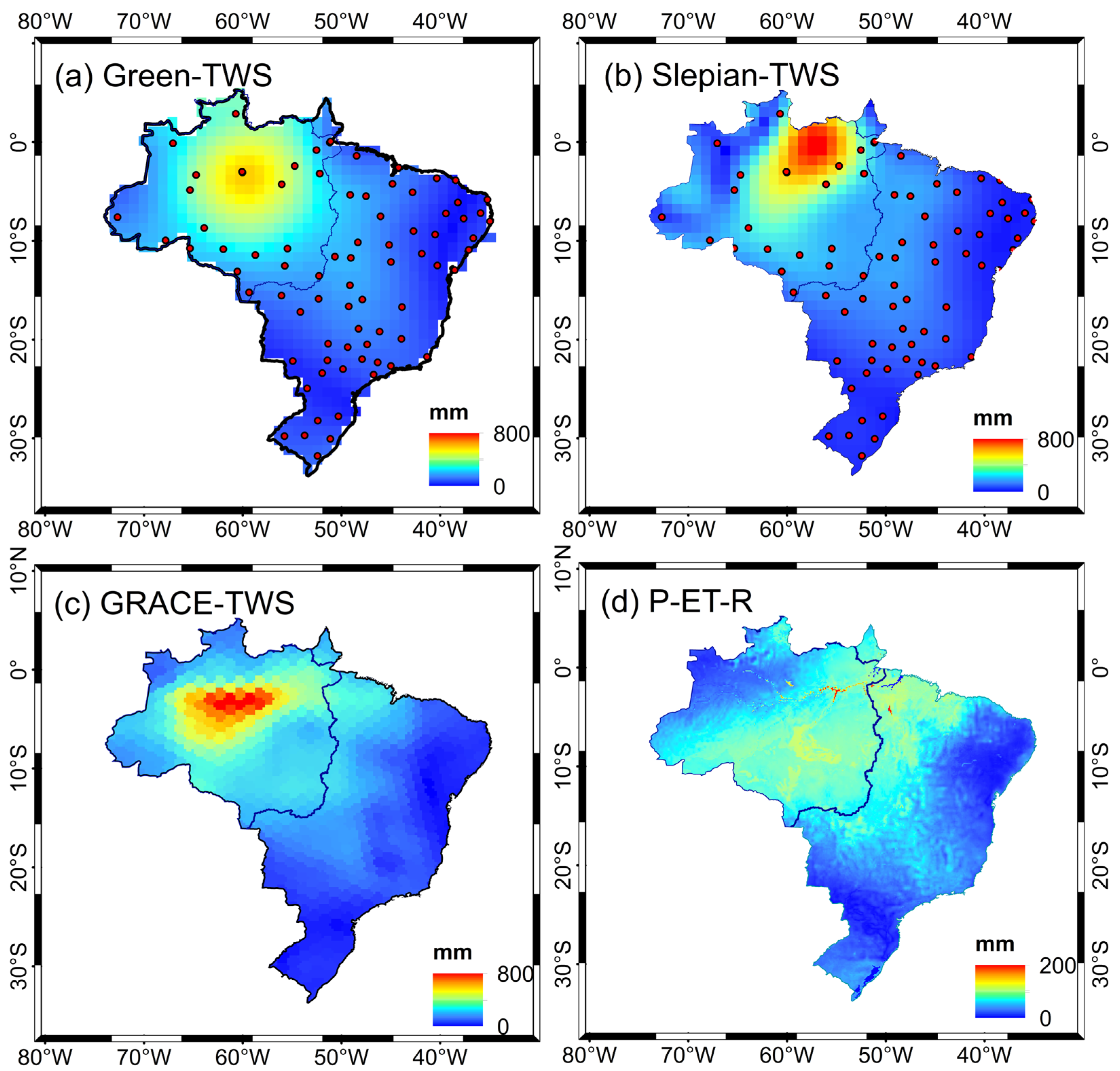
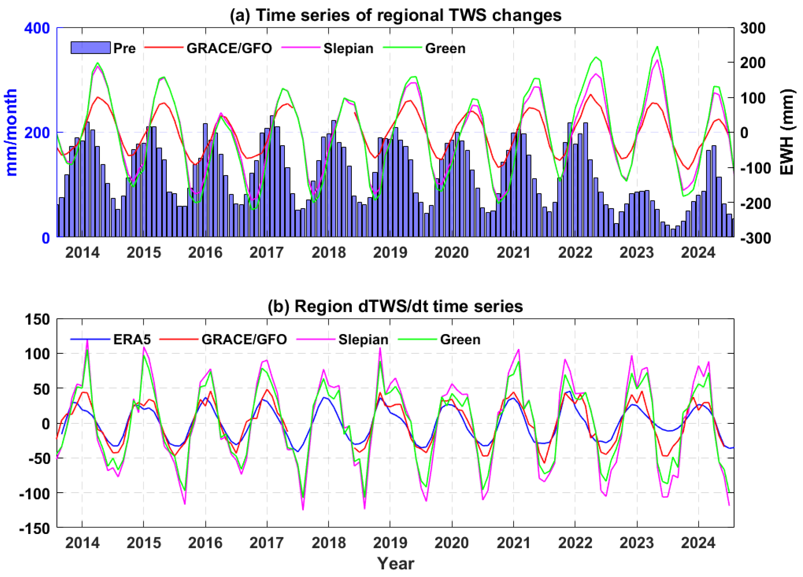
4.2. Spatiotemporal Characteristics of TWS Inversion Using Geodetic Data

To verify the accuracy of the inversion results from different geodetic techniques, this study calculates TWS changes inverted by Green’s function method, the Slepian basis function method, results from GRACE/GFO data, and hydrological data through the water balance equation. Figure 6 reveals that the seasonal fluctuation in TWS in the AMP is significantly more pronounced than in southern Brazil, and the peak of seasonal fluctuation occurs in the middle reaches of the Amazon Basin, which is consistent with the annual amplitude trend of GNSS vertical displacement shown in Figure 5a. This further indicates that the vertical motion amplitude observed at GNSS stations on the Earth’s surface partly reflects the intensity of mass changes within the Earth [25].

Figure 6a,b show the TWS changes individually inferred from GNSS data using different inversion methods. The peak value of Slepian-TWS (~800 mm) is notably higher than that of Green-TWS (~600 mm), likely due to the differences between the inversion methods. Green’s function method inverts TWS by considering all hydrological loads within 50 km around the GNSS station. In contrast, the Slepian basis function method theoretically concentrates the influence of all relevant hydrological loads within this range on the station for calculation. The difference between the two methods becomes more pronounced in areas with significant vertical displacement variations, such as near the Amazon Basin, resulting in a higher peak value of Slepian-TWS than Green-TWS. Figure 6c presents the annual amplitude of TWS changes derived from GRACE/GFO, with a peak value of about 800 mm at the middle reaches of the Amazon Basin. This distribution closely resembles that of Green-TWS. The difference in peak values between GNSS and GRACE/GFO is primarily due to the sparse distribution of GNSS stations in Brazil, with an average distance of about 350 km, resulting in lower GNSS-TWS values, especially near the Amazon Basin, where GNSS stations are minimal. However, the denser distribution of GNSS stations in the southern Brazilian Plateau does not lead to a significant response to hydrological loads; the climate, landscape, and anthropogenic interventions in eastern and southern Brazil are unfavourable for hydrological load storage [10]. The inversion results from both geodetic techniques show a similar spatial distribution and numerical values for the Brazilian Plateau. Moreover, this study also calculates the derivative of terrestrial water storage (dTWS/dt) based on the water balance equation (i.e., P-ET-R) and presents the annual amplitude of dTWS/dt for hydrological interpretation, as shown in Figure 6d. Notably, Figure 6a–c shows the annual amplitude of TWS derived from geodetic methods (GNSS and GRACE), whereas Figure 6d reflects the annual amplitude of the rate of TWS changes (dTWS/dt) rather than the TWS itself. Due to this conceptual and mathematical difference, direct numerical comparison is not appropriate. However, the spatial distribution patterns between the geodetic TWS amplitudes and the dTWS/dt amplitudes exhibit overall consistency, suggesting that both approaches capture similar hydrological signals. This complementary agreement supports the reliability of the results presented in this study.

To further evaluate the effectiveness of geodetic techniques in inverting TWS over large-scale regions, this study calculates the time series of regional TWS and dTWS/dt. As shown in Figure 7a, the TWS changes in Brazil exhibit significant seasonality, and the TWS time series derived from different geodetic techniques present high consistency. Regarding precipitation data, the peak of annual precipitation in Brazil occurs between October and December, corresponding to the spring and summer months, whereas the peak of TWS changes often occurs between November and January, caused by a lag in surface deformation [30]. Furthermore, TWS changes reached their lowest value between 2015 and 2016, coinciding with the impact of the El Niño phenomenon [5,28,32], which caused severe drought events in most parts of Brazil. This suggests that TWS changes can provide valuable insights into regional drought situations.

We found that the regional averaged time series (Figure 7a) may obscure some local features of TWS changes. To further investigate local-scale consistency between different observations, we selected the NAUS station as a representative example and calculated the TWS changes derived from various methods at this station. In addition, we drew the corresponding scatter plots and calculated the correlation coefficients (CC) and standard deviations (STD) between each method, as shown in Figure 8. The results show that the TWS time series derived from the Slepian basis method better agrees with the GRACE/GFO results than Green’s function method. The CC and STD between Slepian and GRACE/GFO are 0.97 and 177.32 mm, compared to 0.96 and 579.06 mm for the Green’s function result. This suggests that the Slepian-TWS estimates are more consistent with GRACE/GFO in large-scale regions with sparse GNSS station coverage. Furthermore, all three time series exhibit mutual correlations exceeding 0.90, indicating strong consistency among the different geodetic techniques.

In addition, this study calculates the time derivative of TWS using both Formula (1) and Formula (7), as shown in Figure 7b. The results indicate that the TWS changes observed using geodetic data closely align with those derived from meteorological and hydrological data, with correlation coefficients around 90%, as presented in

Table 1. Correlation coefficients between dTWS/dt obtained from different datasets.

	Green-TWS	Slepian-TWS	GRACE-TWS	P-ET-R
Green-TWS	-	-	-	-
Slepian-TWS	0.99	-	-	-
GRACE-TWS	0.90	0.90	-	-
P-ET-R	0.87	0.87	0.93	-

. However, the monitoring range of the meteorological and hydrological data is slightly narrower. This limitation arises because TWS changes result from not only precipitation, evapotranspiration, and runoff, but also other factors such as soil moisture dynamics, land use change, and human activities like groundwater extraction and irrigation. These processes interact at different scales and cannot be fully captured by conventional meteorological and hydrological data. During the period 2022–2024, Brazil experienced unique precipitation drought events, and the impacts on TWS were not timely, so a more comprehensive analysis of the drought factors is necessary to investigate the changes in regional drought events in depth.

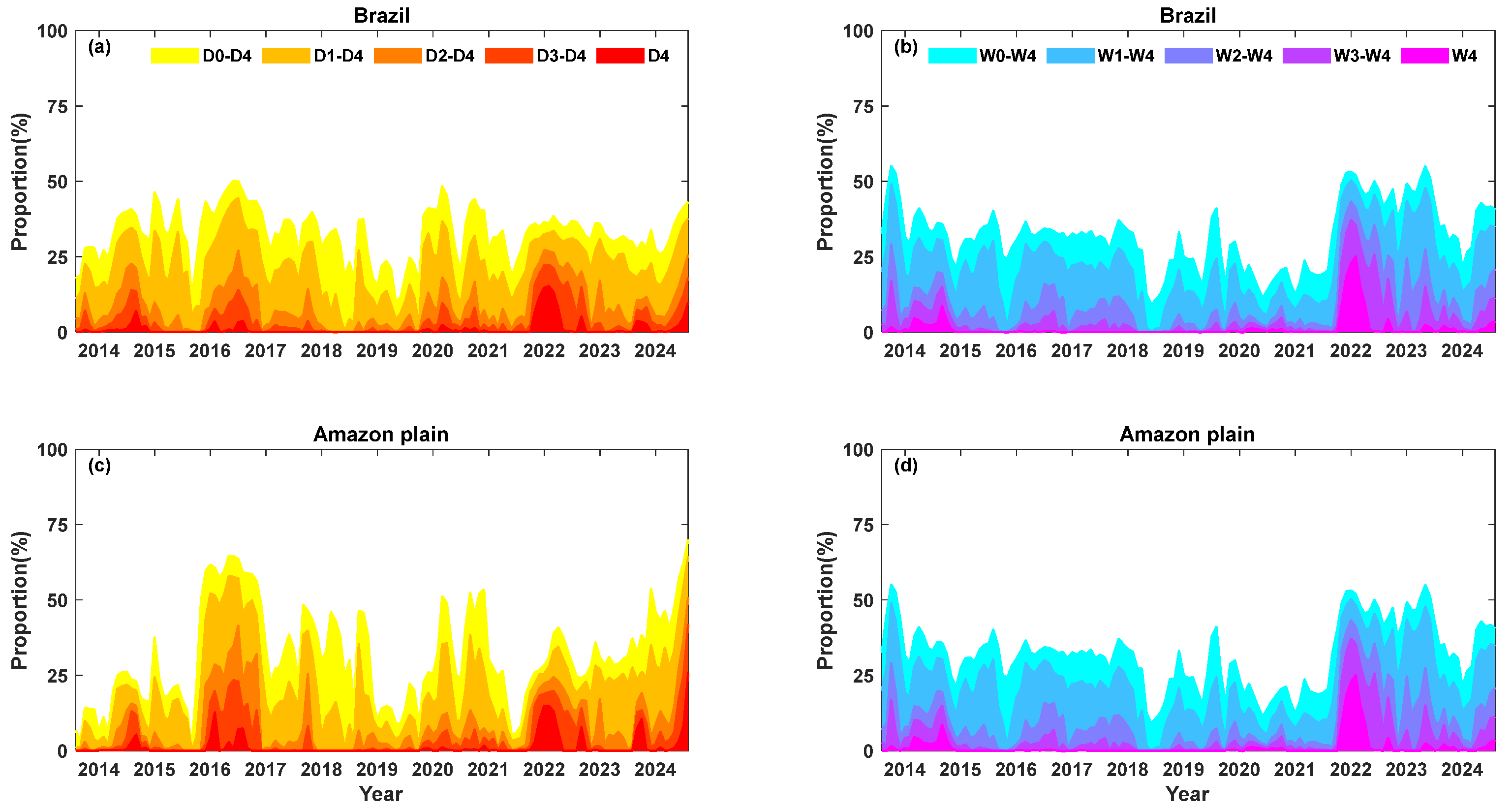
4.3. Hydrological Drought Characteristics Monitoring Using Geodetic Techniques

This study evaluates the spatiotemporal variations of DSI, SPI, and SPEI in Brazil at the same time scale. Figure 9 presents the time series of hydrological and meteorological drought indices on a monthly time scale. According to the drought severity classification proposed by Zhao et al. (2017) [40] (Table S1), this study defines a severe drought event as when the drought index falls below −1.3. The results reveal that Brazil experienced severe drought in four main stages between August 2013 and August 2024 (occurring in October 2015, March 2020, September 2020, and October 2023, respectively). The hydrological and meteorological drought indices exhibited a relatively strong correlation coefficient of about 0.5 during these four severe drought events. To facilitate a more intuitive comparison, Figure 9b and Figure 9c display the drought index time series for 2015–2016 and 2022–2024, respectively. The results indicate that the absolute values of the two GNSS-DSI are significantly higher than other drought indices, likely because GNSS is more sensitive to short-term changes in hydrological signals. Additionally, the meteorological drought index tends to detect drought events earlier, as shown in Figure 9c. The hydrological drought index failed to capture the signal at the onset of the 2023 drought event until May 2023, at which time the GNSS-DSI and GRACE-DSI began to show a decreasing trend. However, SPI and SPEI had already decreased as early as August 2022 when the rainfall deficit began. This suggests that the occurrence of hydrological drought lagged behind the meteorological flux deficit, and these lags are likely associated with the complex dynamic processes involved in water storage and transport [28]. This phenomenon is mainly attributed to the phased and delayed response of hydrological systems to meteorological forcing. Specifically, meteorological drought reflects short-term deficits in precipitation, which can be promptly detected by indices such as SPI and SPEI. In contrast, hydrological drought involves cumulative changes in variables such as soil moisture, groundwater recharge, and terrestrial water storage. These processes are influenced by soil properties, land cover, antecedent wetness, and vegetation water use, leading to a delayed response in hydrological drought indices. Figure S7 also shows the spatial distribution of SPI, SPEI and DSI from January to December 2020. Additionally, GNSS-DSI tends to respond more rapidly to near-surface hydrological changes than GRACE-DSI due to its higher temporal resolution, making it more sensitive in capturing early signals of hydrological drought. This further confirms that hydrological drought signals vary across spatial and temporal scales, depending on the observation system used.

An analysis of the precipitation deficit suggests that the drought events in Brazil from 2013 to 2022 are only weakly related to changes in precipitation and may be due to climate factors, such as the 2015 El Niño event. In contrast, a sharp decline in precipitation primarily drives the drought events that began in 2023. Figure 9d presents the time series of the Niño3.4 index. Periods during which the Niño3.4 index remains greater than or equal to 0.5 or less than or equal to −0.5 for more than five consecutive months are identified as El Niño events. These periods are highlighted with red shading in Figure 9d.

This study defines a drought event as one that occurs when the DSI is less than −0.5 and persists for more than three months.

Table 2. Drought events monitoring in Brazil by different drought indices.

	Occurrence Time	Duration (Month)	DSI Peak	Average DSI	Main Drought Types
Slepian-DSI	November 2015–December 2016	14	−1.95 (June 2016)	−1.38	D2
	January 2020–June 2020	6	−1.73 (April 2020)	−1.06	D1
	August 2020–February 2021	7	−1.40 (September 2020)	−1.06	D1
	December 2023–August 2024	9	−2.23 (August 2024)	−1.00	D1
Green-DSI	November 2015–December 2016	14	−2.06 (July 2016)	−1.48	D2
	March 2018–July 2018	5	−0.83 (May 2018)	−0.67	D0
	January 2020–May 2020	5	−1.44 (April 2020)	−1.00	D1
	August 2020–January 2021	6	−1.26 (September 2020)	−0.85	D1
	December 2023–August 2024	9	−2.09 (August 2024)	−0.82	D1
GRACE/GFO-DSI	November 2015–September 2016	11	−1.79 (June 2016)	−1.42	D2
	September 2023–July 2024	11	−1.97 (March 2024)	−1.59	D2
SPI	May 2021–August 2021	4	−0.74 (all time)	−0.74	D0
	September 2022–August 2024	24	−1.64 (February 2024)	−1.33	D2
SPEI	June 2015–September 2015	4	−1.09 (August 2015)	−0.87	D1
	June 2016–September 2016	4	−1.03 (August 2016)	−0.86	D1
	June 2017–September 2017	4	−1.18 (June 2017)	−0.97	D1
	June 2018–September 2018	4	−1.03 (August 2018)	−0.89	D1
	June 2019–September 2019	4	−1.27 (August 2019)	−0.98	D1
	July 2020–October 2020	4	−1.25 (August 2020)	−1.07	D1
	May 2021–September 2021	4	−1.24 (August 2021)	−1.00	D1
	June 2022–February 2024	21	−1.67 (August 2023)	−1.07	D1

presents the number and severity of drought events in Brazil based on different drought indices from August 2013 to August 2024. A comparison of the meteorological drought index with the hydrological drought index reveals that the drought events identified by the two indices are roughly the same, especially the extreme drought events in 2015, 2019, and 2023. However, the hydrological drought index typically lags behind the meteorological drought index, indicating a delayed response to drought conditions.

The meteorological drought index (e.g., SPEI) exhibits noticeable seasonal fluctuations, especially during the winter season (June to September), with the most severe drought period usually occurring in August. However, the meteorological drought index tends to underestimate drought severity, particularly compared to the hydrological drought index. During the same period, the drought intensity values indicated by SPI and SPEI are generally lower than those derived from GNSS-DSI and GRACE-DSI, which are more sensitive to groundwater losses and provide a more comprehensive assessment of drought impacts. Even if precipitation returns to normal, drought impacts and recovery processes may persist for an extended period, so the meteorological and hydrological drought indices remain valuable for ongoing drought monitoring even after precipitation has normalized. In the subsequent discussion, this study will provide a detailed analysis of the drought events caused by the prolonged precipitation deficit during 2023–2024.

5. Discussion

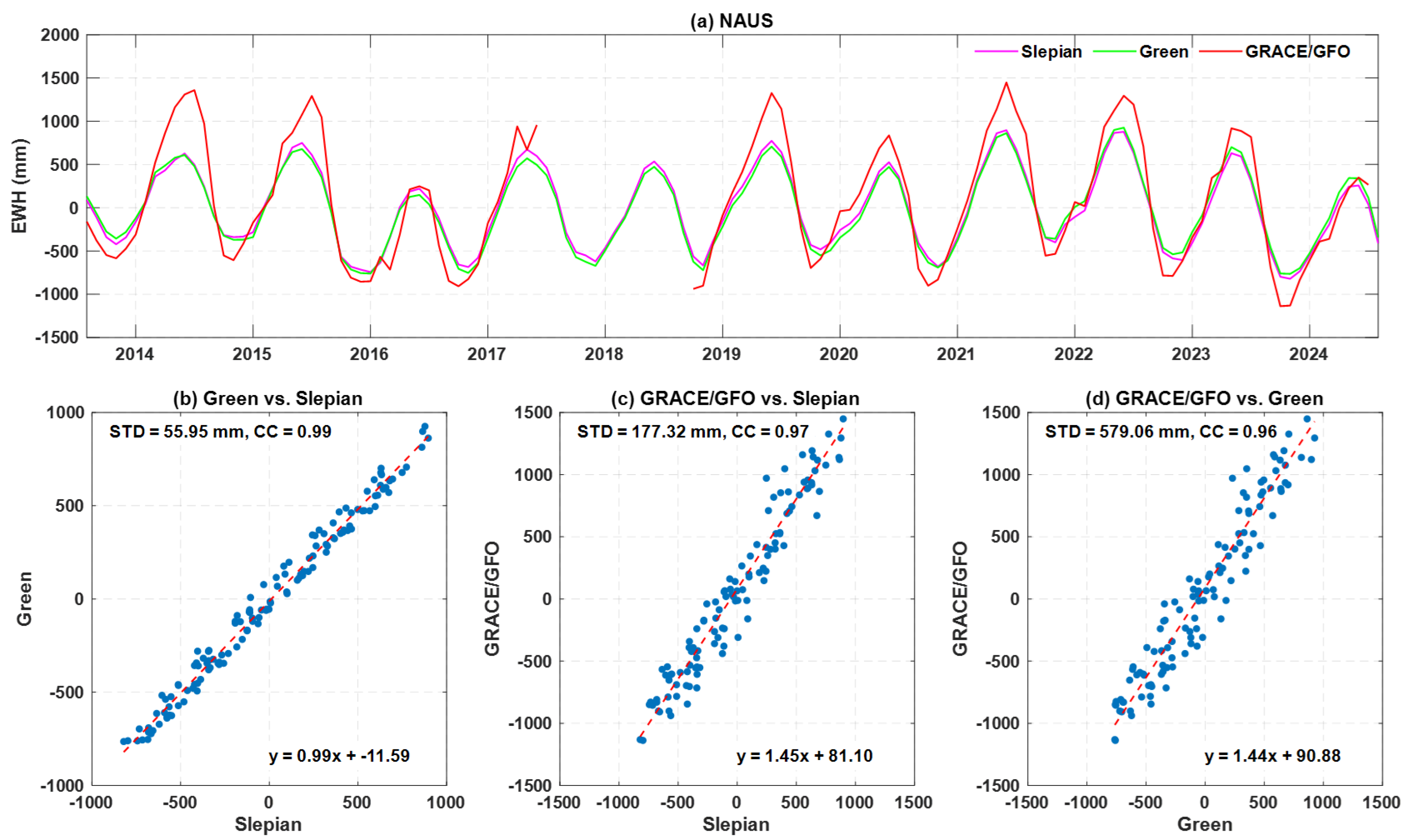
5.1. TWS Variation Characteristics on a Small-Scale Range

As mentioned earlier, the hydrological loads monitored by the GNSS stations in AMP exhibit significant variations (Figure 5a). Therefore, this paper selects AMP in northern Brazil as the study area to conduct a more detailed analysis of the small-scale spatial units represented by this region.

GNSS has been extensively demonstrated to capture details of TWS changes at small spatial scales [15,21,22,24,27]. As shown in Figure 10a, the correlation between GRACE-TWS and GNSS-TWS is extremely high (exceeding 0.9), and the regional average TWS change in AMP is more pronounced than that in the entire Brazil (Figure 7a). This suggests that the TWS change in AMP constitutes a significant portion of the total TWS variation in Brazil. Notably, AMP is a small-scale region, and Brazil is a large-scale one, but the time series variation in Figure 10a is more substantial than that in Figure 7a. This is because this study calculates the TWS change as the regional average across the entire grid. Although Brazil is a large-scale region, the TWS change in its northern part is much more pronounced than in the southern part, where the change is minimal. In contrast, the TWS change across the entire AMP is relatively substantial, leading to a more significant variation, as shown in Figure 10a. Figure 10b illustrates the time series variations of different drought indices in the AMP. The results indicate a strong consistency among the hydrological drought indices (including GRACE-DSI, Green-DSI, and Slepian-DSI), with their amplitude being more pronounced than that of the meteorological drought index. This may be because TWS changes in AMP mainly originate from surface water variations [10], which meteorological drought indices often fail to capture.

Table 3. Monitoring of drought events in Amazon by different drought indices.

	Occurrence Time	Duration (Month)	DSI Peak	Average DSI	Main Drought Types
Slepian-DSI	November 2015–December 2016	14	−2.03 (January 2016)	−1.31	D2
	August 2020–January 2021	6	−1.23 (September 2020)	−0.87	D1
	August 2023–August 2024	13	−2.31 (August 2024)	−1.39	D2
Green-DSI	November 2015–December 2016	14	−2.19 (February 2016)	−1.51	D2
	December 2017–May 2018	6	−0.84 (March 2018)	−0.69	D0
	August 2023–August 2024	13	−2.26 (August 2024)	−1.32	D2
GRACE/GFO-DSI	November 2015–June 2016	8	−1.79 (June 2016)	−1.41	D2
	September 2023–July 2024	11	−1.97 (March 2024)	−1.60	D3
SPI	October 2015–February 2016	5	−0.74 (February 2016)	−0.74	D0
	September 2022–August 2024	24	−1.64 (August 2023)	−1.36	D2
SPEI	July 2015–October 2015	4	−1.41 (September 2015)	−1.04	D1
	July 2020–October 2020	4	−1.26 (August 2020)	−1.07	D1
	June 2021–October 2021	5	−1.12 (August 2021)	−0.75	D0
	July 2022–February 2024	20	−1.71 (September 2023)	−1.18	D1

presents the drought events monitored by different indices, broadly consistent with those in Table 2 for Brazil. For the same drought event, the AMP region exhibits a longer drought duration, higher DSI peaks, and more severe average drought conditions than Brazil. This suggests that the AMP may experience more significant water resource pressures and greater ecological impacts during drought events. As the world’s largest tropical rainforest region, the AMP is highly sensitive to variations in precipitation, and drought periods may substantially affect local vegetation growth, forest fires, and soil moisture. However, the rest of Brazil may demonstrate relatively smaller responses and impacts during drought events due to its geographical location and climatic conditions.

5.2. Quantification of Regional Hydrological Drought Characteristics for 2023–2024

The above results demonstrate a strong correlation between GNSS and GRACE/GFO in terms of time series trends and spatial distribution characteristics. Considering the nearly one-year data gaps between GRACE and GFO, their ability to monitor the frequency of hydrological drought events is limited compared to GNSS. Therefore, this section adopts the results from GNSS for analysis and discussion to provide a more comprehensive analysis of hydrological drought characteristics.

According to Table S1, DSI was divided into five categories representing different levels of drought and humidity [40]. This study then calculated the percentage of the total area in which droughts and floods occurred in Brazil and the AMP from 2013 to 2024, as shown in Figure 11. Besides, this study defined drought frequency as the proportion of months with DSI less than −0.5 over the entire period [30], while flood frequency was defined as the proportion of months with DSI greater than 0.5. Finally, this study investigated the spatial distribution patterns of drought and flood frequencies, as depicted in Figure 12. For Brazil as a whole, severe drought (D2) has been the predominant condition, with about 50% of the country experiencing drought from August 2013 to August 2024. Exceptional drought (D4) was most pronounced during 2016–2017, 2022–2023, and 2024, with about 10%, 15%, and 15% of the country in abnormal drought during these three drought periods. The extreme drought event in 2016 has been proven to be triggered by the process as the heat flow surged into South America during El Niño, leading to air drying and precipitation decreases in AMP, along with atmospheric circulation due to ocean temperatures increasing, thus preventing the typical water transport mechanisms [38].

Droughts in the northeastern AMP are dominated by D2, and a comparison with Figure 12a shows that the timing of droughts in the AMP closely aligns with that of the entire Brazilian region. AMP experienced drought conditions from about half of 2013 to 2023, with periods of concentrated exceptional drought in 2016–2017, 2022–2023, and 2024, when 7%, 15%, and 25% of this region were in exceptional drought. During the period 2023–2024, Figure 12b displays that drought events primarily occurred near the Amazon Basin, mainly due to a sharp decrease in precipitation starting from the second half of 2022. The precipitation deficit lasted 23 months, with an average of −92.13 km³ per month. Despite the recovery of the precipitation deficit by 2024 (Figure 10b and Figure 11b), the prolonged water shortage still led to a gradual increase in drought conditions, and precipitation during the recovery period may not be sufficient to quickly compensate for the long-term water deficit, especially in terms of groundwater recharge and soil moisture recovery. Until August 2024, the drought peaked, with about 75% of AMP in drought and around 25% in D4.

In addition to the impacts of drought, it is priority to consider the adverse effects of flooding in Brazil. During the 2023–2024 period, the intensification of El Niño exacerbated the drought in northeastern Brazil, while precipitation became concentrated in the southeast, leading to persistent flooding in this area (Figure 12d). As shown in Figure 11d, the flood disasters lasted for an extended period, with their severity primarily categorized as moderately wet (W1). This highlights the complexity and interrelatedness of climate extremes in Brazil, where both droughts and floods occur simultaneously, significantly affecting the region’s water resources, agriculture, and overall environmental stability.

6. Conclusions

This study employs different geodetic techniques (including GNSS and GRACE/GFO) to invert the TWS changes across both large-scale regions (e.g., Brazil) and small-scale regions (e.g., AMP), and then investigates the drought conditions during the period 2013–2024 from the perspectives of hydrological and meteorological droughts. The results indicate the following:

(1) The surface deformation observed through GNSS vertical displacement provides insights into regional mass load variations, primarily reflecting fluctuations in hydrological load. In Brazil, the variations in GNSS vertical displacement present a clear trend of gradual attenuation from north to south, with the most significant changes occurring on both sides of the Amazon Basin. This phenomenon may be closely related to alterations in the regional hydrological load, as seasonal precipitation and fluctuations in water volume within the Amazon Basin lead to substantial surface deformation.

(2) The spatiotemporal characteristics of TWS changes obtained by different methods show good consistency, with the correlation coefficients between Green-TWS, Slepian-TWS, and GRACE-TWS all greater than 0.9. TWS changes display clear seasonal patterns, manifested as an increase in precipitation during the summer seasons (November–December), leading to a corresponding rise in TWS. In addition, TWS changes lag behind the precipitation peak by about 2–3 months, due to a result of the complex hydrological processes involved in water transport from precipitation to TWS. Spatially, the oscillations in hydrological load gradually diminish from the northern AMP to the southern Brazilian Plateau.

(3) This study calculates the hydrological and meteorological drought index to monitor drought events, with a correlation coefficient of about 0.5. The meteorological drought index is primarily influenced by meteorological factors, and the calculated SPEI has significant seasonality. Furthermore, the meteorological drought index tends to be more responsive to drought events than the hydrological drought index. The latter usually detects drought events with a lag, as it reflects changes in hydrological conditions over a longer time. However, the hydrological drought index effectively identifies ongoing drought events and provides a more accurate assessment of drought severity, making it particularly suitable for long-term drought monitoring.

(4) This study adopts geodetic techniques to monitor four major drought events in Brazil between 2013 and 2024. The most severe droughts occurred in 2016 and 2024, with about 50% and 40% of the region experiencing drought, respectively. The AMP in northeastern Brazil is the main region affected by these drought events. The drought event in 2024 was primarily driven by a sharp decline in precipitation, during which about 25% of the AMP was in abnormal drought conditions. This highlights the critical role of geodetic technology in drought monitoring, as it provides accurate and timely information on the progression and intensity of drought events in both large-scale and small-scale regions.

Geodetic techniques provide valuable insights into the spatial distribution of drought and its impact on water resources, agriculture, and ecosystems by monitoring surface changes. These techniques, such as GNSS and GRACE/GFO, offer useful information for early warning systems and response strategies. However, the coarse resolution of GRACE/GFO data limits their ability to capture localized drought dynamics, and GNSS-based observations depend heavily on station density, which may affect the reliability of monitoring in regions with sparse coverage. Future research should focus on improving the efficiency and accuracy of drought monitoring by enhancing the GNSS station network, especially in areas with low station density, and exploring the integration of GNSS, GRACE/GFO, and InSAR techniques to address both spatial coverage limitations and temporal resolution. This multi-technique approach is expected to provide more comprehensive support for meeting climate change challenges.

References

1. He, X.G.; Pan, M.; Wei, Z.W.; Wood, E.F.; Sheffield, J. A Global Drought and Flood Catalogue from 1950 to 2016. B. Am. Meteorol. Soc. 2020, 101, E508–E535. [Google Scholar] [CrossRef]
2. Zhu, H.; Chen, K.; Hu, S.; Liu, J.; Shi, H.; Wei, G.; Chai, H.; Li, J.; Wang, T. Using the global navigation satellite system and precipitation data to establish the propagation characteristics of meteorological and hydrological drought in Yunnan, China. Water Resour. Res. 2023, 59, e2022WR033126. [Google Scholar] [CrossRef]
3. Zhang, W.; Lu, X. Inversion Method for Monitoring Daily Variations in Terrestrial Water Storage Changes in the Yellow River Basin Based on GNSS. Water 2024, 16, 1919. [Google Scholar] [CrossRef]
4. Han, Z.; Huang, S.; Huang, Q.; Leng, G.; Wang, H.; Bai, Q.; Zhao, J.; Ma, L.; Wang, L.; Du, M. Propagation dynamics from meteorological to groundwater drought and their possible influence factors. J. Hydro. 2019, 578, 124102. [Google Scholar] [CrossRef]
5. Cunha, A.P.M.A.; Zeri, M.; Leal, K.D.; Costa, L.; Cuartas, L.A.; Marengo, J.A.; Tomasella, J.; Vieira, R.M.; Barbosa, A.A.; Cunningham, C.; et al. Extreme Drought Events over Brazil from 2011 to 2019. Atmosphere 2019, 10, 642. [Google Scholar] [CrossRef]
6. Chen, C.; Zou, R.; Fang, Z.; Cao, J.; Wang, Q. Using geodetic measurements derived terrestrial water storage to investigate the characteristics of drought in Yunnan, China. GPS Solut. 2023, 28, 51. [Google Scholar] [CrossRef]
7. Pintori, F.; Serpelloni, E. Drought-Induced Vertical Displacements and Water Loss in the Po River Basin (Northern Italy) From GNSS Measurements. Earth Spa. Sci. 2024, 11, e2023EA003326. [Google Scholar] [CrossRef]
8. Rodell, M.; Famiglietti, J.S. Detectability of variations in continental water storage from satellite observations of the time dependent gravity field. Water Resour. Res. 1999, 35, 2705–2723. [Google Scholar] [CrossRef]
9. White, A.M.; Gardner, W.P.; Borsa, A.A.; Argus, D.F.; Martens, H.R. A review of GNSS/GPS in hydrogeodesy: Hydrologic loading applications and their implications for water resource research. Water Resour. Res. 2022, 58, e2022WR032078. [Google Scholar] [CrossRef]
10. Feng, W. GRAMAT: A comprehensive Matlab toolbox for estimating global mass variations from GRACE satellite data. Earth Sci. Inform. 2018, 12, 389–404. [Google Scholar] [CrossRef]
11. Luan, K.; Hu, J.; Feng, G.; Qiu, Z.; Zhang, K.; Zhu, W.; Wang, J.; Wang, Z. Terrestrial Water Storage Changes over the Last 20 Years in the Amazon Basin. Sens. Mater. 2022, 34, 4053–4069. [Google Scholar] [CrossRef]
12. Zhong, B.; Li, X.; Li, Q.; Tan, J.; Dai, X. Evaluating the weekly changes in terrestrial water storage estimated by two different inversion strategies in the Amazon River Basin. Geod. Geodyn. 2023, 14, 614–626. [Google Scholar] [CrossRef]
13. Tapley, B.D.; Bettadpur, S.; Ries, J.C.; Thompson, P.F.; Watkins, M.M. GRACE measurements of mass variability in the Earth system. Sci. 2004, 305, 503–505. [Google Scholar] [CrossRef]
14. Thomas, A.C.; Reager, J.T.; Famiglietti, J.S.; Rodell, M. A GRACE- based water storage deficit approach for hydrological drought characterization. Geophys. Res. Lett. 2014, 41, 1537–1545. [Google Scholar] [CrossRef]
15. Argus, D.F.; Fu, Y.N.; Landerer, F.W. Seasonal variation in total water storage in California inferred from GPS observations of vertical land motion. Geophys. Res. Lett. 2014, 41, 1971–1980. [Google Scholar] [CrossRef]
16. Carlson, G.; Werth, S.; Shirzaei, M. Joint Inversion of GNSS and GRACE for Terrestrial Water Storage Change in California. J. Geophys. Res. Solid Earth 2022, 127, e2021JB023135. [Google Scholar] [CrossRef]
17. Carlson, G.; Werth, S.; Shirzaei, M. A novel hybrid GNSS, GRACE, and InSAR joint inversion approach to constrain water loss during a record-setting drought in California. Remote Sens. Environ. 2024, 311, 114303. [Google Scholar] [CrossRef]
18. Fu, Y.N.; Argus, D.F.; Landerer, F.W. GPS as an independent measurement to estimate terrestrial water storage variations in Washington and Oregon. J. Geophys. Res. Solid Earth 2015, 120, 552–566. [Google Scholar] [CrossRef]
19. Han, S.-C.; Razeghi, S.M. GPS Recovery of Daily Hydrologic and Atmospheric Mass Variation: A Methodology and Results from the Australian Continent. J. Geophys. Res. Solid Earth 2017, 122, 9328–9343. [Google Scholar] [CrossRef]
20. Jiang, Z.S.; Tang, M.; Yang, X.H.; Wen, H.P.; Yuan, L.G.; Shen, Y.C.; Feng, W.; Zhong, M. Characterizing multifarious hydroclimatic patterns using geodetic measurements in the Australian mainland. J. Hydrol. 2024, 642, 131792. [Google Scholar] [CrossRef]
21. Fok, H.S.; Liu, Y. An improved GPS-inferred seasonal terrestrial water storage using terrain-corrected vertical crustal displacements constrained by GRACE. Remote Sens. 2019, 11, 1433. [Google Scholar] [CrossRef]
22. Li, X.P.; Zhong, B.; Li, J.C.; Liu, R.L. Inversion of GNSS Vertical Displacements for Terrestrial Water Storage Changes Using Slepian Basis Functions. Earth Space Sci. 2023, 10, e2022EA002608. [Google Scholar] [CrossRef]
23. Yang, X.; Yuan, L.; Jiang, Z.; Tang, M.; Feng, X.; Li, C. Investigating terrestrial water storage changes in Southwest China by integrating GNSS and GRACE/GRACE-FO observations. J. Hydrol. Reg. Stud. 2023, 48, 101457. [Google Scholar] [CrossRef]
24. Li, X.P.; Zhong, B.; Li, J.C.; Liu, R.L. Joint inversion of GNSS and GRACE/GFO data for terrestrial water storage changes in the Yangtze River Basin. Geophys. J. Int. 2023, 233, 1596–1616. [Google Scholar] [CrossRef]
25. Farrell, W.E. Deformation of the Earth by surface loads. Rev. Geophys. 1972, 10, 761–797. [Google Scholar] [CrossRef]
26. Blewitt, G.; Lavallée, D.; Clarke, P.; Nurutdinov, K. A new global mode of Earth deformation: Seasonal cycle detected. Science 2001, 294, 2342–2345. [Google Scholar] [CrossRef] [PubMed]
27. Jiang, Z.S.; Hsu, Y.-J.; Yuan, L.G.; Huang, D.F. Monitoring time-varying terrestrial water storage changes using daily GNSS measurements in Yunnan, southwest China. Remote Sen. Environ. 2021, 254, 112249. [Google Scholar] [CrossRef]
28. Tang, M.; Yuan, L.; Jiang, Z.; Yang, X.; Li, C.; Li, W. Characterization of hydrological droughts in Brazil usinga novel multiscale index from GNSS. J. Hydrol. 2023, 617, 128934. [Google Scholar] [CrossRef]
29. Qiu, K.; You, W.; Jiang, Z.; Tang, M. Tracking the water storage and runoff variations in the Parana ’ basin via GNSS measurements. Sci. Total Environ. 2023, 912, 168831. [Google Scholar] [CrossRef]
30. Peng, Y.J.; Chen, G.; Chao, N.F.; Wang, Z.T.; Wu, T.T.; Luo, X.Y. Detection of extreme hydrological droughts in the poyang lake basin during 2021–2022 using GNSS-derived daily terrestrial water storage anomalies. Sci. Total Environ. 2024, 919, 170875. [Google Scholar] [CrossRef]
31. Li, X.P.; Zhong, B.; Chen, J.L.; Cheng Li, J.; Wang, H.H. Investigation of 2020–2022 extreme floods and droughts in Sichuan Province of China based on joint inversion of GNSS and GRACE/GFO data. J. Hydrol. 2024, 2024, 130868. [Google Scholar] [CrossRef]
32. Jiang, Z.; Hsu, Y.-J.; Yuan, L.; Cheng, S.; Feng, W.; Tang, M.; Yang, X. Insights into hydrological drought characteristics using GNSS-inferred large-scale terrestrial water storage deficits. Earth Planet. Sci. Lett. 2022, 578, 117294. [Google Scholar] [CrossRef]
33. Blewitt, G.; Hammond, W.; Kreemer, C. Harnessing the GPS Data Explosion for Interdisciplinary Science. Eos 2018, 99, e2020943118. [Google Scholar] [CrossRef]
34. Dill, R.; Dobslaw, H. Numerical simulations of global-scale high-resolution hydrological crustal deformations. J. Geophys. Res. Solid Earth 2013, 118, 5008–5017. [Google Scholar] [CrossRef]
35. Liu, N.; Dai, W.J.; Santerre, R.; Kuang, C.L. A MATLAB-based Kriged Kalman Filter software for interpolating missing data in GNSS coordinate time series. GPS Solut. 2018, 22, 25. [Google Scholar] [CrossRef]
36. Save, H.; Bettadpur, S.; Tapley, B.D. High-resolution CSR GRACE RL05 mascons. J. Geophys. Res. Solid Earth 2016, 121, 7547–7569. [Google Scholar] [CrossRef]
37. Muñoz Sabater, J. ERA5-Land Hourly Data from 1950 to Present; Copernicus Climate Change Service (C3S) Climate Data Store (CDS): Berkshire, UK, 2019. [Google Scholar] [CrossRef]
38. Chen, J.; Tapley, B.; Rodell, M.; Seo, K.W.; Wilson, C.; Scanlon, B.R.; Pokhrel, Y. Basin-Scale River Runoff Estimation From GRACE Gravity Satellites, Climate Models, and In Situ Observations: A Case Study in the Amazon Basin. Water Resour. Res. 2020, 56, e2020WR028032. [Google Scholar] [CrossRef]
39. Landerer, F.W.; Dickey, J.O.; Güntner, A. Terrestrial water budget of the Eurasian pan-Arctic from GRACE satellite measurements during 2003–2009. J. Geophys. Res. Atmos. 2010, 115, D23. [Google Scholar] [CrossRef]
40. Zhao, M.; Aa, G.; Velicogna, I.; Kimball, J.S. Satellite Observations of Regional Drought Severity in the Continental United States Using GRACE-Based Terrestrial Water Storage Changes. J. Clim. 2017, 30, 6297–6308. [Google Scholar] [CrossRef]
Figure 1. Geographical map of Brazil. The green dots are GNSS stations; the blue lines are main rivers with digital elevation data in the background.
Remotesensing 17 01670 g001
Figure 2. (a) Annual amplitude of precipitation data in Brazil; (be) time series of meteorological and hydrological data for Brazil, including precipitation, evapotranspiration, runoff, and temperature.
Remotesensing 17 01670 g002
Figure 3. Research flowchart.
Remotesensing 17 01670 g003
Figure 4. Temporal and spatial functions of GNSS hydrological load by PCA decomposition.
Remotesensing 17 01670 g004
Figure 5. Spatial distribution of annual amplitude (a) and phase (b) of GNSS vertical crustal displacements.
Remotesensing 17 01670 g005
Figure 6. Spatial distribution of TWS annual amplitude obtained from different data sources, the red dots represent GNSS stations: (a) Green-TWS; (b) Slepian-TWS; (c) GRACE-TWS; (d) dTWS/dt inferred by P-ET-R.
Remotesensing 17 01670 g006
Figure 7. (a) Time series of regional TWS changes obtained from different datasets; (b) time series of regional dTWS/dt derived from different datasets.
Remotesensing 17 01670 g007
Figure 8. (ad) Time series and scatter plot comparison of TWS changes at NAUS station (August 2013–August 2024) derived from Green’s function method, the Slepian basis function method, and GRACE/GFO. The red dotted line in (bd) represents the linear regression fitting line.
Remotesensing 17 01670 g008
Figure 9. (a) Time series of various drought indices in Brazil during 2013–2024. (b) Time series of various drought indices in Brazil during 2015–2016. (c) Time series of various drought indices in Brazil during 2022–2024. (d) Time series of Niño3.4, where the red areas represent the periods when El Niño events occurred.
Remotesensing 17 01670 g009
Figure 10. Hydrological characteristics in AMP: (a) time series of regional TWS changes obtained from different datasets; (b) time series of drought indices derived from different datasets.
Remotesensing 17 01670 g010
Figure 11. (a,b) Proportion of droughts and floods in Brazil; (c,d) proportion of droughts and floods in AMP.
Remotesensing 17 01670 g011
Figure 12. Frequency of droughts and floods in Brazil during the periods 2013–2024 and 2023–2024. (a) represents the drought frequency in Brazil from 2013 to 2024, (b) represents the drought frequency in Brazil from 2023 to 2024, (c) represents the flood frequency in Brazil from 2013 to 2024, and (d) represents the flood frequency in Brazil from 2023 to 2024.
Remotesensing 17 01670 g012