SPIFFNet: A Statistical Prediction Interval-Guided Feature Fusion Network for SAR and Optical Image Classification

Abstract

The problem of the feature extraction and fusion classification of optical and SAR data remains challenging due to the differences in optical and synthetic aperture radar (SAR) imaging mechanisms. To this end, a statistical prediction interval-guided feature fusion network, SPIFFNet, is proposed for optical and SAR image classification. It consists of two modules, the feature propagation module (FPM) and the feature fusion module (FFM). Specifically, FPM imposes restrictions on the scale factor of the batch normalization (BN) layer by means of statistical prediction interval, and features exceeding the scale factor of the interval are considered redundant and are replaced by features from other modalities to improve the classification accuracy and enhance the information interaction. In the feature fusion stage, we combine channel attention (CA), spatial attention (SA), and multiscale squeeze enhanced axial attention (MSEA) to propose FFM to improve and fuse cross-modal features in a multiscale cross-learning manner. To counteract category imbalance, we also implement a weighted cross-entropy loss function. Extensive experiments on three optical–SAR datasets show that SPIFFNet exhibits excellent performance.

1. Introduction

The advancement of sensor technology has facilitated the acquisition of substantial multi-platform and multi-modal remote sensing data [1,2,3]. Among the most critical types of imagery in remote sensing are optical and synthetic aperture radar (SAR) images, which have been increasingly studied. Optical sensors, characterized by their extensive spectral capabilities, can capture data across various bands, including visible light, near infrared, and short-wave infrared [4]. However, optical imagery is vulnerable to weather conditions. In contrast, SAR employs microwave imaging [5], which is impervious to weather influences, enabling continuous operation under all weather conditions and offering a certain degree of penetration [6]. However, SAR images are more difficult to interpret due to the complexity of the imaging mechanism. Consequently, merging optical data with SAR data effectively can improve multiple Earth observation activities, like classifying land cover [7], change detection [8], target extraction [9], and so on.

Since deep learning technology has been applied to the field of remote sensing image classification [10], innovative network architectures have been developed to enhance the efficiency of deep learning techniques, including convolutional neural networks (CNNs), [11], recurrent neural networks (RNNs) [12], graph neural networks (GNNs) [13], and generative adversarial networks (GANs) [14]. In earlier studies, due to the backwardness of earth observation capabilities and sensor technology, researchers usually focused on the classification of single-source remote sensing images. The authors of [15] use deep learning technology, and a real-valued parameter convolutional neural network is proposed to directly classify complex-valued SAR data. Nonetheless, convolutional neural networks have limitations that prevent them from effectively extracting texture features. The authors of [16] address the issue of classifying heterogeneous SAR images using transfer learning. Although it can learn effective domain invariant features, the model cannot be widely used, because SAR images themselves lack rich spectral information. Recently, some methods have been proposed to combine multimodal data to improve classification performance. The authors of [17] first designed CNN to extract deep features of multi-source images simultaneously and then used SVM instead of SoftMax to obtain classification results. However, the single-branch design makes this method unable to extract spectral information and texture features simultaneously. In [18], Jiaxin Lu et al. proposed a superpixel segmentation algorithm, which first uses the PCA method to extract optical and SAR features and then uses a multiscale superpixel segmentation algorithm for lithology classification. However, due to the limitations of the PCA algorithm, the model may ignore some effective features or extract too many redundant features. In [19], Xuchu Yu et al. employed both the transformer’s ability to model long-range features and the convolutional neural network’s ability to extract local features at the same time, used the spectral transformer structure to extract the global spectral dependency in hyperspectral images, dynamically integrated spectral and spatial features through the feature coupling module, and finally, designed a multilevel network architecture to extract hierarchical features. However, the parallel feature extraction architecture adopted by the dynamic coupling strategy results in a lack of direct interaction between multimodal features, which may ignore the correlation between cross-modal features. At the same time, the fusion position is late, which may lead to information loss or insufficient fusion, and a more complex fusion mechanism is required to fully utilize the information.

The joint classification of optical and SAR images [20] can be divided into the following two stages: the first stage is feature extraction, and the second stage is feature fusion. Therefore, how to effectively and accurately extract spectral and spatial features and fuse them is crucial for the classification task. The authors of [21] utilized parallel multiscale spectral and spatial attention modules along residual paths to emphasize discriminative features and suppress redundancy, followed by a multilevel convolutional fusion module to refine integration. However, this methods lacks explicit mechanisms for cross-modal feature interaction at the propagation stage, relying mainly on attention within a single modality. The authors of [22] employed dual encoders to process SAR and optical features separately, integrated a detail attention module for fine structure enhancement, and introduced a compound loss function to reduce noise and address class imbalance. It processed SAR and optical data in isolated encoders and enhanced details post-encoding but lacked an explicit mechanism for mutual feature refinement across domains.

Although the above methods are very helpful for optical and SAR image classification, there are still some problems. Studies have shown that the interaction between optical and SAR features can effectively compensate for the limitations of their respective features, thereby effectively improving classification accuracy. Most existing studies rely on fixed or separate attention mechanisms to extract features from different modalities. However, these approaches often treat modalities independently or in parallel, without dynamically assessing the usefulness of features during extraction. This leads to the following two major issues: redundant or noisy features are preserved, and the lack of interaction between SAR and optical features at the early stage weakens cross-modal complementarity. Moreover, fusion strategies in existing networks are typically implemented as a late-stage integration step. These methods do not establish strong dependencies between spatial and spectral domains or between modalities in a progressive manner. They lack the dynamic modulation or feedback to adaptively guide fusion based on the relevance and informativeness of the features. Therefore, to address the above issues, we introduce a feature propagation strategy that constrains the scale factor of BN through a statistical prediction interval, allowing the early filtering of redundant information and replacing it with complementary information from other modalities. This cross-modal interaction during feature extraction enhances the discriminative ability. At the same time, we combine spatial attention, channel attention, and multiscale axial attention in the feature fusion stage to form a tightly integrated fusion strategy that captures global context and fine-grained features more effectively than traditional fusion blocks. The significant contributions of this research are as follows:

(1)

A combined classification model is developed for classifying optical and SAR images. The feature propagation block is used to extract the spectral spatial features of optical and SAR images. The weight-sharing method is used to reduce the number of training parameters, improve the training performance of the model, and enhance the generalization ability.

(2)

Using a statistical prediction interval to limit the scale factor of the BN layer is conducive to extracting complementary features and reducing redundant information, giving full play to the complementary advantages of optics and SAR.

(3)

A feature fusion module is designed to help the model concentrate on detailed features and to build long-range dependencies, integrating the advantages of optics and SAR and further improving the classification ability of the model.

The rest of the paper is organized as follows: Section 2 presents the specific details of the proposed SPIFFNet. Experimental results and data on three datasets are analyzed in Section 3. A discussion is presented in Section 4. In Section 5, we summarize our paper Some additional information on data distribution is given in Appendix A

2. Proposed Framework

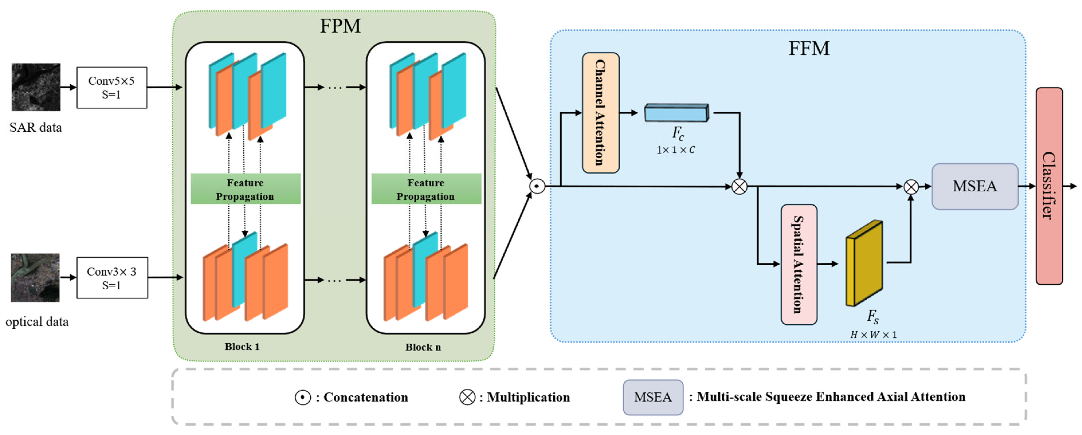
This section provides a detailed overview of SPIFFNet. Figure 1 illustrates the architecture of the proposed SPIFFNet framework, which is composed of two primary components, FPM and FFM. First, n blocks are used to extract features from SAR data and optical data, respectively, and the two types of data are interacted based on the statistical prediction interval method, which is feature propagation. Secondly, CA, SA, and MSEA constitute FFM. The channel refinement features $F_c$ extracted by channel attention and the spatial refinement features $F_s$ extracted by the spatial attention module are multiplied with the input features to further enhance both types of features. Subsequently, MSEA is employed to cross-learn and fuse the two types of features, so that the optical and SAR features form complementary strengths. Finally, the classification results are obtained using a SoftMax classifier.

2.1. Feature Propagation Module

2.1.1. Feature Extraction Based on Block

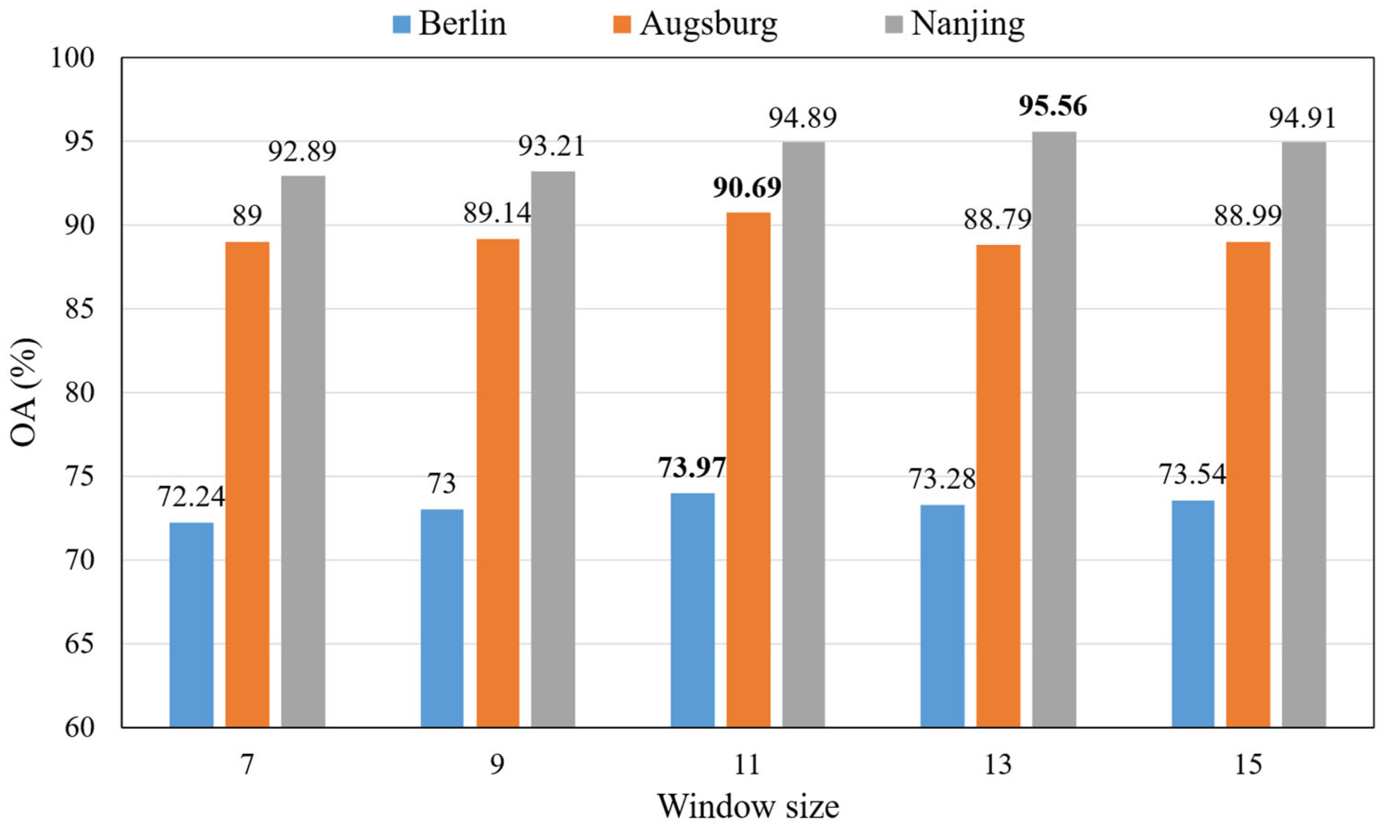
In order to facilitate the extraction of classification features, we used a $w\times w$ size spatial neighbourhood window to represent the central pixel. Therefore, the input SAR image and optical image can be described as $X_{\mathrm{s}\mathrm{a}\mathrm{r}}\in {\mathbb{R}}^{w\times w\times c_s}$ and $X_{\mathrm{o}\mathrm{p}\mathrm{t}}\in {\mathbb{R}}^{w\times w\times c_o}$, where $w$ represents the window size, and $c_s$ and $c_o$ are the channel number of SAR and optical data.

The $\mathrm{C}\mathrm{o}\mathrm{n}\mathrm{v}3\times 3$ and $\mathrm{C}\mathrm{o}\mathrm{n}\mathrm{v}5\times 5$ of the first layer of the SPIFFNet are employed to adjust the optical and SAR data to the same dimensions. Optical images usually contain rich colors and detailed features [23], and smaller convolution kernels can better capture local features and subtle changes, while SAR images usually have strong noise and complex textures [24], and using slightly larger convolution kernels can help the network better capture the overall structural and textural information, while reducing the effect of noise. Therefore, we choose $\mathrm{C}\mathrm{o}\mathrm{n}\mathrm{v}3\times 3$ and $\mathrm{C}\mathrm{o}\mathrm{n}\mathrm{v}5\times 5$ to extract optical and SAR features, respectively. The size of the original image patch remains unchanged with $\mathrm{C}\mathrm{o}\mathrm{n}\mathrm{v}3\times 3$ and $\mathrm{C}\mathrm{o}\mathrm{n}\mathrm{v}5\times 5$, with only the channel number being modified. Afterwards, n blocks are used to extract spectral and spatial features. These blocks share common weights. This design can greatly reduce the number of parameters that need to be learned and reduce the risk of overfitting [25]. 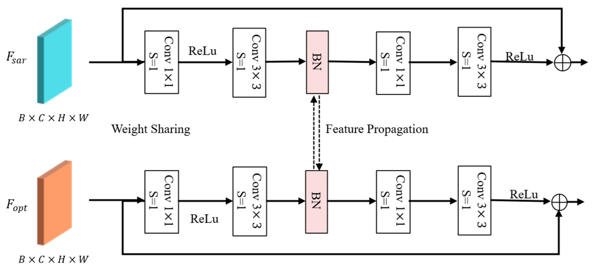Figure 2 illustrates the detailed structure of the block, which includes multiple convolutional layers with varying kernel sizes and batch normalization layers. We use the ReLu activation function, because it is simple to implement and performs well in various classification tasks. In the BN layer, feature propagation is achieved by limiting the scale factor of the independent BN layer. The parameters of the BN layer do not share weights and are trained independently. In addition, the block also uses residual operations to overcome the gradient fading [26] problem caused by the increase in the number of model layers. Therefore, while retaining the characteristics of the two types of data, the classification performance of the model is improved.

In addition, we used the stochastic gradient descent (SGD) optimization algorithm, which can search for the best parameters to minimize the loss function. In order to deal with the problem of the imbalanced number of training samples, we used the weighted cross-entropy loss function. At the same time, in order to avoid overfitting the model, we also added the $L_1$ regularization term to the loss function [27]. The loss function at the end can be described as follows:

$$loss=-\sum _{i=1}^C{\omega }_i{y}_{i}log{\widehat{y}}_i+\lambda \sum _{n=1}^N\sum _{l=1}^L\left|{\gamma }_{n,l}\right|$$

(1)

where ${\omega }_i$ represents the weight of label $i$, calculated according to the proportion of label $i$ within the total sample. For example, when the total number of samples is $T$, and there are $C$ different labels, the number of samples with label $i$ is represented as $t_i$, then ${\omega }_i=T/(C\times t_i)$. $y_i$ and ${\widehat{y}}_i$ represent the true label and the output of the model, respectively. $N$ and $L$ are the number of data sources and BN layers. $\lambda$ is the regularization constant, and $\gamma$ is the scale factor of the BN layer.

2.1.2. Feature Propagation Based on Statistical Prediction Interval

One of the reasons why deep learning network models are difficult to train is that the model contains many hidden layers. As training progresses, the parameters of each layer are modified and optimized, resulting in a continuous change in the input distribution of the hidden layer, which causes each hidden layer to encounter covariate shift [28]. However, batch normalization, a popular and effective technique, can consistently accelerate the convergence of deep networks [29]. BN transforms $X$ according to the following expression:

$$\mathrm{y}=\gamma \widehat{\mathrm{x}}+\beta =\gamma {\displaystyle \frac{\mathrm{x}-\mu }{\sqrt{{\sigma }^2+\epsilon }}}+\beta$$

(2)

where $\mathrm{x}\in {\mathbb{R}}^{B\times C\times H\times W}$ represents the SAR or optical feature of the input. After BN operation, $\mathrm{y}\in {\mathbb{R}}^{B\times C\times H\times W}$. $\mu$ is the mean of $\mathrm{x}$, and ${\sigma }^2$ is the variance of $\mathrm{x}$. $\epsilon$ is a small constant to ensure that the denominator is not 0. $\gamma$ and $\beta$ are the scale factor and shift factor, respectively.

During the training process, the change range of the middle layer should not be too drastic, and the BN operation makes the distribution of each layer actively centered. Therefore, we limited the scale factor. In fact, too large or too small a scale factor will have a bad effect on the convergence of the model. If the loss function is too large, the model parameters will be updated too quickly, so that the optimal solution cannot be found. 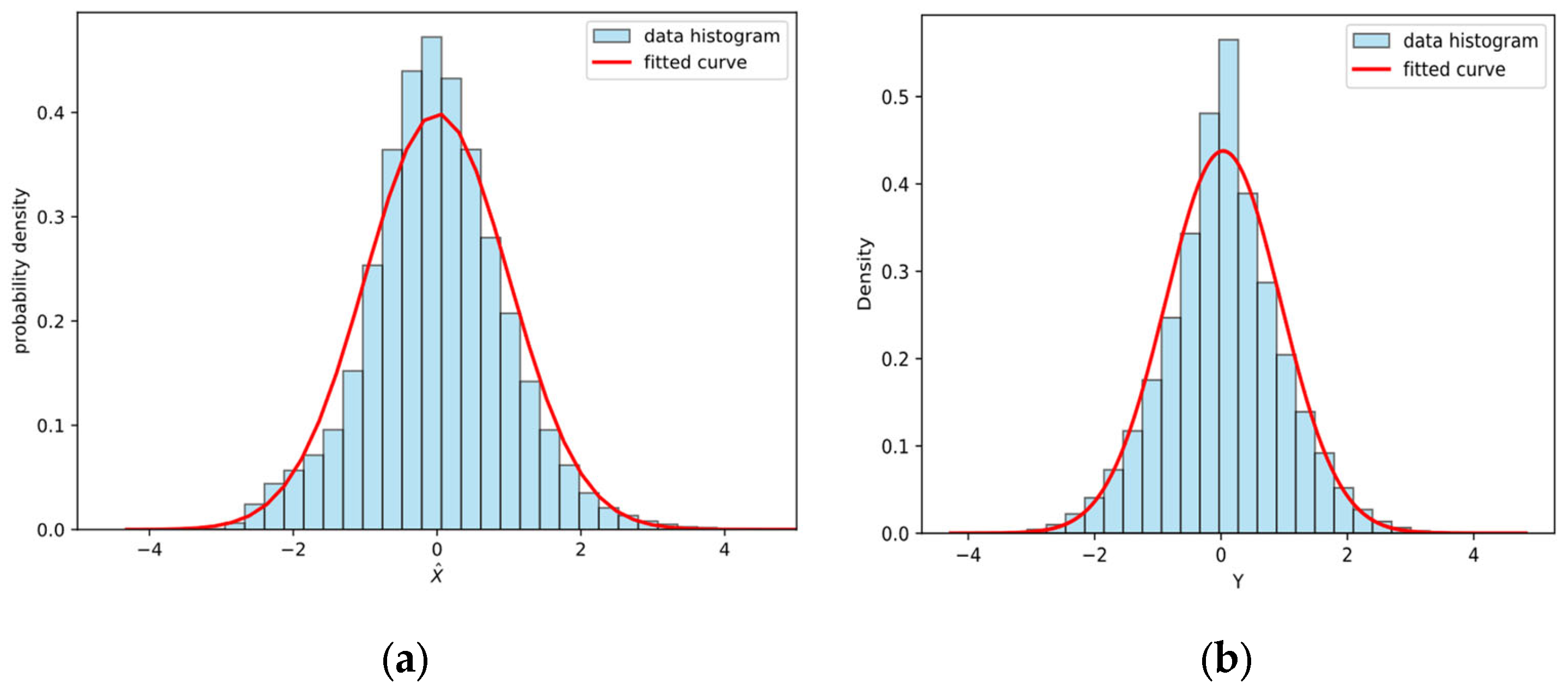If the loss function is too small, the model parameters will be updated too slowly and may fall into the local optimization [30], which will be analyzed in detail in Section 2.3. Following the standard in batch normalization [31], the feature activations after BN are considered to be approximately following a standard normal distribution. At the same time, we analyzed the post-BN distribution of our features and observed that they approximately follow a normal-like shape (see Figure A1 in Appendix A). Equation (2) shows that $\widehat{\mathrm{x}}$ follows a standard normal distribution, that is, $X\sim N\left(\mathrm{0,1}\right)$. Because $X$ follows a standard normal distribution, $Y$ also follows a normal distribution. From Equation (3), we can obtain the mean of $Y$ as $\beta$ and the variance as ${\gamma }^2$.

$$\begin{gathered} \hspace{0.33em}E\left[Y\right]=E[\gamma X+\beta ]=\gamma E\left[X\right]+\beta =\beta \\ D\left[Y\right]=D[\gamma X+\beta ]={\gamma }^{2}D\left[X\right]={\gamma }^2 \end{gathered}$$

(3)

Therefore, we can obtain $Y\sim N(\beta ,{\gamma }^2)$ and define the sample mean and sample variance as follows:

$$\begin{gathered} \hspace{0.33em}\overline{Y}={\displaystyle \frac{1}{n}}\sum _{i=1}^n{Y}_i \\ {S}^2={\displaystyle \frac{1}{n-1}}\sum _{i=1}^n(Y_i-\overline{Y}{)}^2={\displaystyle \frac{1}{n-1}}\left(\sum _{i=1}^n{Y}_i^2-n{\overline{Y}}^2\right) \end{gathered}$$

(4)

where $n$ is the total number of sample. $\overline{Y}$ and $S^2$ are the sample mean and sample variance, respectively.

For the sample mean $\overline{Y}$ and sample variance $S^2$ of a Gaussian random variable $Y$, it follows from [32] that they satisfy, as follows:

$${\displaystyle \frac{\left(n-1\right)S^2}{{\gamma }^2}}\sim {\chi }^2\left(n-1\right)$$

(5)

where $\overline{Y}$ and $S^2$ are independent of each other. ${\chi }^2(n-1)$ represents ${\chi }^2$ distribution with degree of freedom $n-1$.

Figure 3 shows the probability density of the ${\chi }^2$ distribution with $n-1$ degrees of freedom. Point ${\chi }_{\alpha /2}^2(n-1)$ is the upper $\alpha /2$ quantile of ${\chi }^2(n-1)$. Therefore, the probability of the shaded area is calculated as follows:

$$\begin{gathered} P\left\{{\chi }_{1-{\displaystyle \frac{\alpha }{2}}}^2\left(n-1\right)<{\displaystyle \frac{\left(n-1\right)S^2}{{\gamma }^2}}<{\chi }_{{\displaystyle \frac{\alpha }{2}}}^2\left(n-1\right)\right\}=1-\alpha \\ P\left\{{\displaystyle \frac{\left(n-1\right)S^2}{{\chi }_{\frac{\alpha }{2}}^2\left(n-1\right)}}<{\gamma }^2<{\displaystyle \frac{\left(n-1\right)S^2}{{\chi }_{1-\frac{\alpha }{2}}^2\left(n-1\right)}}\right\}=1-\alpha \end{gathered}$$

(6)

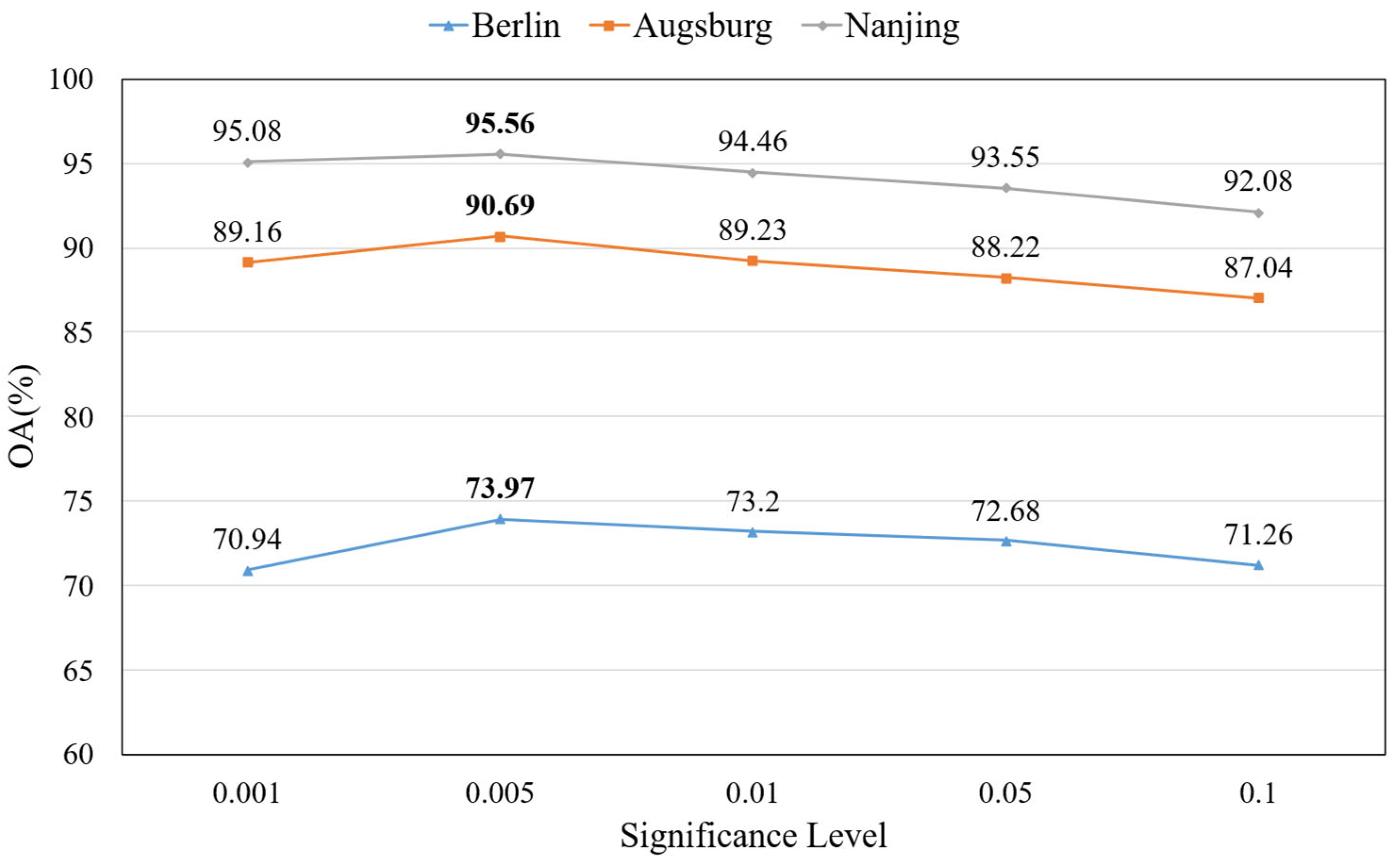
The range of the scale factor is calculated by the statistical prediction interval method. Equation (6) shows a confidence interval of the variance of the Gaussian variable $Y$ with a confidence level of $1-\alpha$, that is, the confidence interval of scale factor ${\gamma }^2$.$\alpha$ represents the significance level.

During model training, the scale factor $\gamma$ for each channel is learned along with other model parameters, as the input features pass through the BN layer. The scale factor of each channel of the SAR or optical feature is compared to the scale factor interval range obtained from Equation (6). If the $\gamma$ of the current channel is within the interval range, that is, ${\gamma }^2\in D$, then the feature of the current channel is considered to contribute to the subsequent classification and is a useful feature, and if the $\gamma$ of the current channel is too large or too small, resulting in exceeding this interval range, that is, ${\gamma }^2\notin D$, then the feature of the current channel is detrimental to the subsequent classification of the model, which is analysed in detail in Section 2.3. Therefore, it can be considered that the features of the current channel are redundant features, and the current features should be replaced with features from another data source, which is the process of feature propagation. Taking optical characteristics as an example, the specific process of feature propagation is described as follows:

$$\begin{gathered} {\mathbf{y}}_{opt}=\left\{\begin{array}{ll}{\gamma }_{opt}{\displaystyle \frac{{\mathbf{x}}_{opt}-{\mu }_{opt}}{\sqrt{{\sigma }_{opt}^2+\epsilon }}}+{\beta }_{opt},& if {\gamma }_{opt}^2\in D\\ {\gamma }_{sar}{\displaystyle \frac{{\mathbf{x}}_{sar}-{\mu }_{sar}}{\sqrt{{\sigma }_{sar}^2+\epsilon }}}+{\beta }_{sar},& else\end{array}\right. \\ D=\left({\displaystyle \frac{\left(n-1\right)S^2}{{\chi }_{\frac{\alpha }{2}}^2\left(n-1\right)}},{\displaystyle \frac{\left(n-1\right)S^2}{{\chi }_{1-\frac{\alpha }{2}}^2\left(n-1\right)}}\right) \end{gathered}$$

(7)

2.2. Feature Fusion Module

After using block for feature propagation, the features between optical and SAR fully interacted, while retaining their advantages. In order to facilitate the subsequent classification, we designed a feature fusion module to combine optical and SAR features, capture global and detailed features, and improve the performance and generalization ability of the model [33]. Initially, the FFM extracts both channel and spatial attention, from the perspectives of channel and space, respectively, to further augment the interaction between optical and SAR data. Then, the MSEA module is used to cross-learn and fuse the two types of features, so that the two types of data complement each other and, thus, improve classification accuracy.

2.2.1. Channel Attention and Spatial Attention

The framework of CA and SA is shown in Figure 4. With the development of deep learning, pooling operations have been increasingly used. Pooling operations can usually reduce the scale of data and aggregate information [34].

As the number of neural network layers increases, the receptive field of each neuron will become larger due to the pooling operation. Pooling operations include maximum pooling and average pooling [35]. Channel attention and spatial attention use both pooling operations at the same time, aggregating the information extracted by the two in different ways and using convolution operations to refine the extracted features further. Ultimately, the channel attention feature map and the spatial attention feature map are derived and subsequently combined with the input feature map through element-wise multiplication.

For channel attention, the calculation process is as follows:

$$\begin{gathered} {\mathrm{F}}_c=\sigma \left(\mathrm{W}\left(Avg\left({\mathrm{F}}_{in}\right)\right)+\mathrm{W}\left(Max\left({\mathrm{F}}_{in}\right)\right)\right) \\ =\sigma \left(Conv\left(\mathrm{R}\mathrm{e}\mathrm{L}\mathrm{u}\left(Conv\left(Avg\left({\mathrm{F}}_{in}\right)\right)\right)\right)+Conv\left(\mathrm{R}\mathrm{e}\mathrm{L}\mathrm{u}\left(Conv\left(Max\left({\mathrm{F}}_{in}\right)\right)\right)\right)\right) \end{gathered}$$

(8)

where ${\mathrm{F}}_{in}\in {\mathbb{R}}^{H\times W\times C}$ is the input feature, and $\sigma$ is sigmoid activation function. The $Avg$ and $Max$ pooling operations here are along the $H$ and $W$ directions and do not change the size of $C$, so ${\mathrm{F}}_c\in {\mathbb{R}}^{1\times 1\times C}$.

$$\begin{gathered} {\mathrm{F}}_s=\sigma \left(Conv\left(\left[Avg\left({\mathrm{F}}_{on}\right);Max\left({\mathrm{F}}_{on}\right)\right]\right)\right) \\ =\sigma \left(Conv\left(\left[Avg\left({\mathrm{F}}_{in}\otimes {\mathrm{F}}_c\right);Max\left({\mathrm{F}}_{in}\otimes {\mathrm{F}}_c\right)\right]\right)\right) \end{gathered}$$

(9)

where ${\mathrm{F}}_{on}\in {\mathbb{R}}^{H\times W\times C}$ is the input feature of spatial attention. $\left[Avg\left(·\right);Max\left(·\right)\right]$ represents concatenating $Avg(·)$ and $Max(·)$ in the channel dimension. The $Avg$ and $Max$ pooling operations here are along the $C$ directions and do not change the size of $H$ and $W$, so ${\mathrm{F}}_s\in {\mathbb{R}}^{H\times W\times 1}$.

2.2.2. Multiscale Squeeze Enhanced Axial Attention

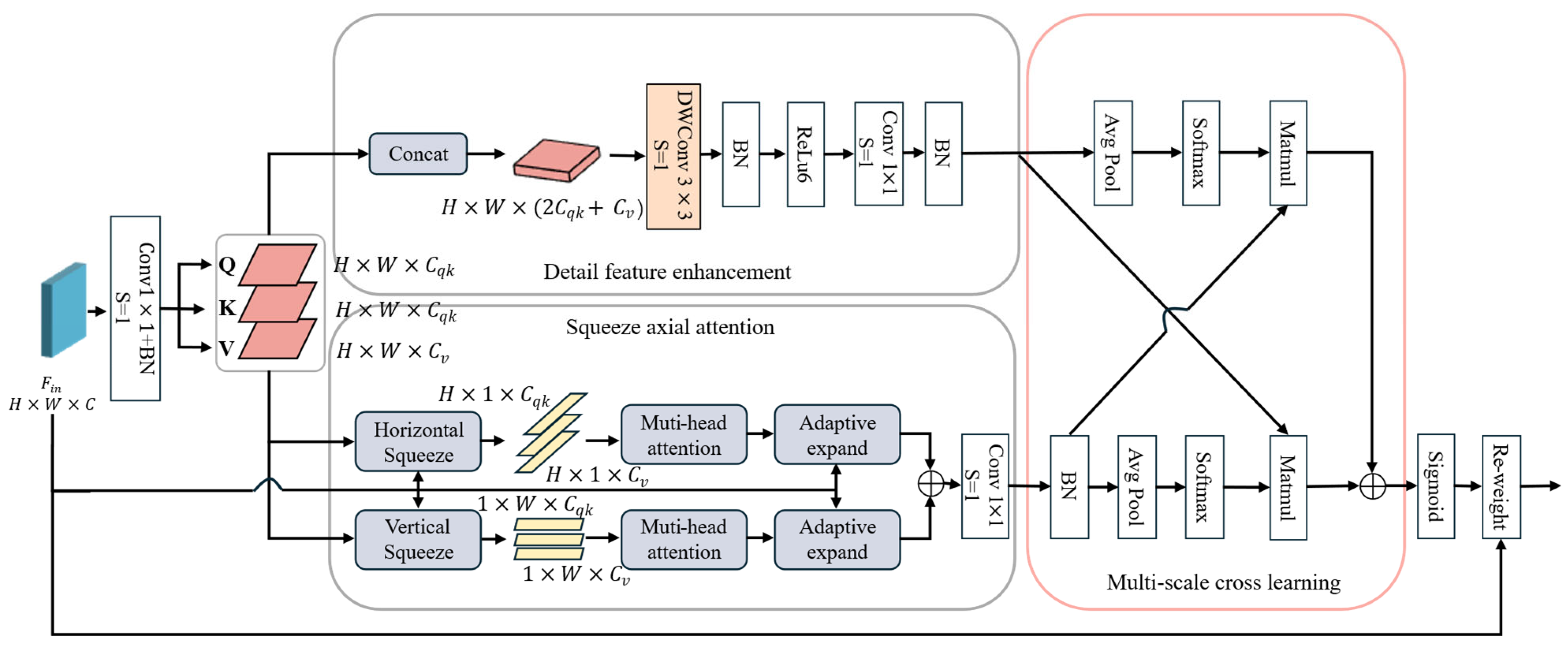
To effectively and accurately fuse and extract more features that are beneficial to classification, inspired by the literature [36], we designed a multiscale squeeze enhanced axial attention, which is shown in Figure 5. In this paper, firstly, the input features passed through a convolution layer and a batch normalization layer to obtain three feature matrices of $\mathrm{Q},\mathrm{K}\in {\mathbb{R}}^{H\times W\times C_{qk}}$, and $\mathrm{V}\in {\mathbb{R}}^{H\times W\times C_v}$. MSEA is improved based on squeezing axial attention similar to the self-attention mechanism. The self-attention mechanism involves the operation between query, key, and value, so its linear complexity is high [37]. 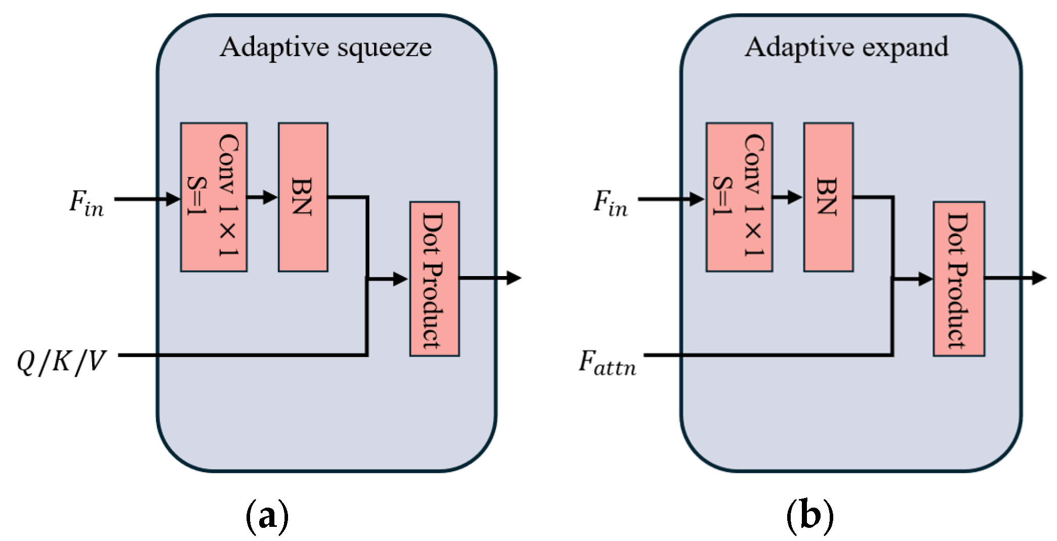With ongoing advancements in remote sensing technology, the data to be processed by the model are also increasing, which makes the calculation cost of the self-attention mechanism increase significantly [38]. Therefore, squeeze axial attention reduces the dimension of data through adaptive squeeze and expansion operations and adds position information, thus improving the calculation speed and accuracy of the model. In contrast to the pooling operation used for compression and broadcasting for expansion, adaptive squeezing and expanding operations enable the model to gather spatial information in an input-adaptive manner, while avoiding significant increases in computational costs. The specific implementation process is shown in Figure 6.

The calculation of squeeze axial attention can be expressed as:

$$y\left(i,j\right)=\sum _{n=1}^{H}softma{x}_n\left({\mathrm{q}}_{\left(h\right)i}^T{\mathrm{k}}_{\left(h\right)n}\right){\mathrm{v}}_{\left(h\right)n}+\sum _{n=1}^{W}softma{x}_n\left({\mathrm{q}}_{\left(v\right)j}^T{\mathrm{k}}_{\left(v\right)n}\right){\mathrm{v}}_{\left(v\right)n}$$

(10)

where ${\mathrm{q}}_{\left(h\right)}$, ${\mathrm{k}}_{\left(h\right)}\in {\mathbb{R}}^{H\times C_{qk}}$, and ${\mathrm{v}}_{\left(h\right)}\in {\mathbb{R}}^{H\times C_v}$ are the result of horizontal squeeze, and ${\mathrm{q}}_{\left(v\right)}$, ${\mathrm{k}}_{\left(v\right)}\in {\mathbb{R}}^{W\times C_{qk}}$, and ${\mathrm{v}}_{\left(v\right)}\in {\mathbb{R}}^{W\times C_v}$ are the result of vertical squeeze.

In order to extract more detailed features, the squeeze axial attention adds a detail feature enhancement branch. The depthwise separable convolution with $3\times 3$ convolution kernel is used to capture multiscale feature representation and extract detail features with a large receptive field [39]. After the feature extraction of the two branches, the features of the two branches need to be efficiently integrated to improve the classification effect of the integrated features [40]. In contrast to existing methods that often rely on single-scale feature interaction or simple concatenation for multimodal fusion, the core innovation of our approach lies in the introduction of a multiscale cross learning fusion mechanism. This design allows features extracted at different scales to interact, complementing global semantic cues with fine-grained spatial information. Such cross-scale interactions significantly enhance the robustness of feature representations, especially when dealing with heterogeneous data sources, such as SAR and optical imagery, which often exhibit modality-specific noise and resolution discrepancies. Therefore, we added multiscale cross learning at the end, using two-dimensional global average pooling to encode global information and establish long-range dependencies and using cross-learning to aggregate two different spatial attention weights. Finally, the learned attention was fused into the input features through the Re-weight method to achieve feature fusion. The Re-weight operation is calculated as follows:

$$y\left(i,j\right)=x\left(i,j\right)\times \mathrm{g}\left(i,j\right)$$

(11)

where $\mathrm{x}\in {\mathbb{R}}^{H\times W\times C}$ denotes the input feature for MSEA, while $\mathrm{g}\in {\mathbb{R}}^{H\times W\times C}$ signifies the attention weight.

2.3. Analysis of Scale Factor

In this paper, we employ the method of statistical prediction interval to impose constraints on the scale factor. In the event that the features of the current channel exceed the specified interval, we regard these features as superfluous information, which will have a detrimental impact on the subsequent classification. To prove that the scale factor is too large or too small, it has a bad effect on the extraction of optical and SAR features. From (1) and (2), the gradient of $x$ can be calculated as follows:

$${\displaystyle \frac{\partial L}{\partial x}}={\displaystyle \frac{\partial L}{\partial y}}{\displaystyle \frac{\partial y}{\partial x}}={\displaystyle \frac{\partial L}{\partial y}}{\displaystyle \frac{\partial y}{\partial \widehat{x}}}{\displaystyle \frac{\partial \widehat{x}}{\partial x}}={\displaystyle \frac{\partial L}{\partial y}}\cdot \gamma \cdot \left({\displaystyle \frac{\partial \widehat{x}}{\partial \mu }}{\displaystyle \frac{\partial \mu }{\partial x}}+{\displaystyle \frac{\partial \widehat{x}}{\partial \sigma }}{\displaystyle \frac{\partial \sigma }{\partial x}}+{\displaystyle \frac{\partial \widehat{x}}{\partial x}}\right)$$

(12)

From (12), the size of the scale factor affects the parameter update of the optical and SAR feature extraction model. At the same time, there is no shift factor in the gradient of $x$, so we only limit the scale factor $\gamma$. When the scale factor is too large, that is $\gamma \to \infty$, this denotes that the loss function is especially sensitive to shifts in the current input feature. The process of feature extraction is intended to capture the distinctive features of optical and SAR. At this stage, the update speed of the parameters is too fast, which will make feature extraction difficult. Conversely, when the scale factor is too minimal, that is $\gamma \to 0$, then $\partial L/\partial x\to 0$, indicating that the current feature does not affect the update of the model parameters. Therefore, the current feature is considered to be a redundant feature, and feature propagation should be performed.

3. Experimental Result and Analysis

3.1. Dataset Introduction and Evaluation Indicators

These datasets include two hyperspectral-SAR (HSI-SAR) datasets, namely the Berlin and Augsburg datasets, and one optical RGB-SAR dataset, namely the Nanjing dataset. The ground truth maps and regional maps of the three datasets are shown in Figure 7.

Table 1. Division of the three datasets into training and testing.

		Berlin Dataset		Augsburg Dataset		Nanjing Dataset
Class		Number of Sample		Number of Sample		Number of Sample
No.	Name	Train	Test	Train	Test	Train	Test
1	Forest	443	54,511	146	13,361	483	176,112
2	Residential Area	423	268,219	264	30,065	579	75,050
3	Industrial Area	499	19,067	21	3830	414	41,472
4	Low Plants	376	58,906	248	26,609	392	39,660
5	Allotment	280	13,025	52	523	\	\
6	Commercial Area	298	24,526	7	1638	\	\
7	Water	170	602	23	1507	293	94,931
8	Soil	331	17,095	\	\	\	\
9	Road	\	\	\	\	129	5863
Total		2820	461,851	761	77,533	2290	433,088

shows the count of randomly chosen training and testing samples for each of the three datasets.

3.1.1. Berlin Dataset

The first dataset is the Berlin HSI-SAR dataset, which covers the urban area of Berlin and nearby country areas. In particular, the HSI data are analogue EnMAP data of size $797\times 220$ pixels synthesized on the basis of HyMap HS data, which contains 244 spectral bands from $0.4 \mathsf{\mu }\mathrm{m}$ to $2.5 \mathsf{\mu }\mathrm{m}$. Meanwhile, the SAR data are Sentinel-1 dual-polarized (VV-VH) single look complex (SLC) data acquired from ESA. Firstly, the SAR data were preprocessed using SNAP software, version 9.0, and the process mainly included apply orbit profile, radiometric calibration, deburst, speckle filtering, terrain correction, and region clipping. Finally, it was saved in the form of a covariance matrix. The size of the SAR data was $1723\times 476$. In order to match the HSI data with the SAR, the nearest neighbor interpolation was performed on the HSI data so as to achieve the same size as the SAR data. There are eight categories in the Berlin dataset: forest, residential area, industrial area, low plants, allotment, commercial area, water, and soil.

3.1.2. Augsburg Dataset

The second dataset is the publicly available Augsburg HSI-SAR dataset [41], which contains three data sources, namely HSI data collected by DAS-EOC, DSM data collected by DLR, and PolSAR data collected by Sentinel-1, polarized with dual polarization (VV-VH). In our experiments, we used both HSI data and SAR data to verify the excellent performance of our model for optical–SAR data classification. The resolution of this dataset is 30 m GSD, and the size is $332\times 485$. The HSI contains 180 spectral bands in the spectral range of $0.4 \mathsf{\mu }\mathrm{m}$ to $2.5 \mathsf{\mu }\mathrm{m}$. The Augsburg dataset has seven classes, which are forest, residential area, industrial area, low plants, allotment, commercial area, and water.

3.1.3. Nanjing Dataset

The third dataset is the Nanjing RGB-SAR dataset, which covers Nanjing, Jiangsu Province, and its surrounding areas. The geographic location of the center of the study area is 32°04′57″N, 118°50′06″E. The SAR image data were acquired by the Canadian RADARSAT-2 satellite with a resolution of 5 m on 17 April 2017, in the form of single look complex data (SLC), and polarized with full polarization. The optical image is a number of images with a resolution of 5 m captured by the German Rapideye satellite in April 2017 and stitched together to form a large map of Nanjing. The preprocessing process is similar to the previous dataset, including apply orbit profile, radiometric calibration, deburst, speckle filtering, terrain correction, and region clipping. Finally, the optical and SAR datasets were cropped to $1500\times 1500$ size. The Nanjing dataset has six classes, which are forest, residential area, industrial area, low plants, water, and road.

3.1.4. Evaluation Indicators

To objectively assess the performance of the proposed method, three widely used evaluation metrics were adopted: overall accuracy (OA), average accuracy (AA), and the Kappa coefficient. These metrics comprehensively reflect the global classification performance.

OA measures the proportion of correctly classified samples to the total number of samples. It provides an intuitive evaluation of the model’s overall classification capability across the entire dataset.

$$OA={\displaystyle \frac{\sum _{i=1}^C{N}_{ic}}{N}}$$

(13)

where $C$ represents the total number of classes, $N_{ic}$ is the number of correctly classified samples for class $i$, and $N$ denotes the total number of samples.

AA refers to the average classification accuracy of each category in the classification task. It can be calculated by dividing the number of correct classifications for each category by the total number of samples in each category.

$$AA={\displaystyle \frac{1}{C}}{\displaystyle \frac{\sum _{i=1}^C{N}_{ic}}{N_i}}$$

(14)

where $N_i$ is the total number of samples belonging to class $i$. This metric reflects the balance of classification performance across all classes.

The Kappa coefficient evaluates the agreement between the predicted labels and the ground truth. A higher Kappa value indicates better classification reliability and consistency, especially in datasets where some classes may dominate the distribution.

$$Kappa={\displaystyle \frac{OA-P_e}{1-P_e}}$$

(15)

where $P_e$ is the expected agreement by chance, calculated as follows:

$$P_e={\displaystyle \frac{\sum _{i=1}^C(N_{i.}\times N_{.i})}{N^2}}$$

(16)

where $N_{i.}$ and $N_{.i}$ represent the total number of samples predicted as class $i$ and the actual number of samples of class $i$, respectively. The Kappa coefficient ranges from −1 to 1, with 1 indicating perfect agreement and values close to 0 suggesting random prediction.

These metrics together enable a comprehensive and fair evaluation of the proposed model, ensuring that both global performance and class-specific classification capabilities are accurately assessed.

3.2. Model Parameter Selected

3.2.1. The Number of Blocks

During the feature propagation phase of SPIFFNet, we designed several feature propagation blocks. In this section, we analyze the impact of the number of blocks on the performance of SPIFFNet. As shown in Figure 8, we conducted experiments by setting the number of blocks to 1, 2, 3, 4, and 5 and obtained the relationship between overall accuracy (OA) and the number of blocks. If the number of blocks is too small, the feature extraction and propagation between optical and SAR data will be insufficient, leading to SPIFFNet failing to capture adequate spectral and spatial features from optical and SAR data, which in turn, degrades its performance. Conversely, if the number of blocks is too large, it will make the depth of SPIFFNet too great, which not only reduces the computational efficiency but also increases the risk of overfitting, thereby decreasing the accuracy of SPIFFNet. In conclusion, selecting an appropriate number of blocks is crucial for SPIFFNet. For the three datasets, the optimal number of blocks is 2.

3.2.2. Significance Level

From Figure 3 and Equation (7), the significance level α affects the estimation accuracy of the statistical prediction interval, that is, the size of the interval $D$, and the size of the interval $D$ determines the feature propagation strategy, so the significance level is also important for model performance. As a key factor, we selected the significance levels of 0.001, 0.005, 0.01, 0.05, and 0.1 for experiments, and the results are shown in Figure 9. When α is larger, the range of interval $D$ will become smaller. As a result, there are too many scale factors that are not within this interval, so the features currently helpful for classification are considered redundant and replaced. This will lead to a lack of useful spectral and spatial features, thus reducing the classification performance. However, a too small $\alpha$ will also have a negative impact. When $\alpha$ is too small, the range of interval $D$ will be larger, which will cause the model to be unable to find redundant features. Therefore, OA will decrease. Through a lot of experiments, the optimal choice is $\alpha =0.005$.

3.2.3. Window Size

In this paper, a window of size $w\times w$ is used to represent the area surrounding the central pixel, and it is evident that the selection of $w$ is also a key factor affecting the classification performance of SPIFFNet. We analyzed the window sizes of 7, 9, 11, 13, and 15 pixels, with the results shown in Figure 10. The larger the window size, the more contextual information around the target can be considered, but a too large window will introduce more noise and increase the computational overhead of the model. The smaller the window, the more the model can focus on some local information, but a too small window may lose the global information of the target. Therefore, for the Berlin and Augsburg datasets, their image size is small, and the spatial resolution is low, and the performance is optimal when $w$ is 11, while for the Nanjing dataset, its image size is large and the spatial resolution is high, and the performance is optimal when $w$ is 13. Furthermore, to guarantee the precision of the experiments, all three datasets were conducted in an identical setting. The outcomes of each experiment were derived from the mean of multiple repetitions of the same experiment.

3.3. Analysis of Experimental Results

In this section, we conducted objective and fair experiments on the proposed method. In order to verify the performance of the proposed SPIFFNet for optical and SAR image classification, we compared it with several other state-of-the-art networks, including MCANet [42], SepDGConv [43], SpectralFormer [44], and AsyFFNet [45]. In detail, MCANet comprises a pseudo-Siamese feature extraction module, a multimodal cross-attention module, and a low–high-level feature fusion module. These components facilitate the avoidance of noise interference and the efficient extraction of multiscale features, while enabling the realisation of the second-order interaction of the attention graph. SepDGConv represents an advancement over dynamic group convolution (DGConv). It permits the hyperparameters of GConv and the entire network architecture to become class-learned throughout the training period of the network. This approach can be applied to any mainstream convolutional network architecture. The SpectralFormer employs a cross-layer jump connection mechanism from the perspective of the transformer order, which is capable of capturing the spectral local sequence information of neighboring bands of an optical image. This approach effectively reduces the information loss that occurs during hierarchical propagation. The AsyFFNet system initially employs a weight-sharing residual block for feature extraction, while imposing constraints on certain scale factors of the BN layer. Subsequently, a feature calibration module is devised to further leverage the spatial correlation of the multi-source data, thereby facilitating the extraction of categorizable features in an efficient manner. To ensure the fairness of the experiments, all experiments were run in the same environment.

3.3.1. Experiments on Berlin Dataset

This paper verifies the performance of SPIFFNet from the following two aspects: objective evaluation indicators and classification maps. For the Berlin dataset, the classification maps of different models are shown in Figure 11. In addition,

Table 2. Classification accuracy (%) of different models on the Berlin dataset.

Class	Performance (%)
	MCANet	SepDGConv	SpectralFormer	AsyFFNet	SPIFFnet
Forest	59.95	68.25	74.75	76.65	75.68
Residential Area	73.38	70.85	67.19	70.76	74.75
Industrial Area	34.15	39.26	68.01	60.16	56.56
Low Plants	77.11	74.70	75.86	74.66	83.52
Soil	68.88	68.26	81.94	79.18	84.62
Allotment	66.39	25.47	82.35	79.24	73.92
Commercial Area	24.96	34.02	35.54	37.94	43.01
Water	57.98	53.05	81.30	83.90	80.67
OA	67.50	68.21	68.72	70.51	73.97
AA	57.85	54.23	70.87	70.31	71.60
Kappa	0.5274	0.5418	0.5663	0.5842	0.6243

gives the three evaluation indicators of these models and the classification accuracy of each class. We can see that the proposed method is significantly better than other methods. Specifically, SPIFFNet improves the overall accuracy of MCANet, SepDGConv, SpectralFormer, and AsyFFNet by 6.47%,5.76%, 5.25%, and 3.46%, respectively. The overall accuracy of the proposed method on the Berlin dataset reached 73.97%, the average accuracy reached 71.60, and the Kappa index reached 0.6243. In addition, we can see that SPIFFNet handles imbalanced data better than other networks, especially in the commercial area category. Due to the small number of training samples, the classification accuracy of other networks is low, but the classification accuracy of SPIFFNet can reach 43.01%, which proves that it can fully extract detailed features and, thus, improve classification performance.

3.3.2. Experiments on Augsburg Dataset

Table 3. Classification accuracy (%) of different models on the Augsburg dataset.

Class	Performance (%)
	MCANet	SepDGConv	SpectralFormer	AsyFFNet	SPIFFNet
Forest	84.66	96.20	95.04	96.72	95.66
Residential Area	84.05	91.77	96.46	96.93	98.02
Industrial Area	68.46	63.52	54.75	48.93	47.18
Low Plants	89.37	82.14	88.60	88.62	94.00
Allotment	31.74	66.92	65.01	76.29	71.76
Commercial Area	19.90	17.95	21.98	28.33	28.79
Water	13.54	48.24	47.11	48.31	48.77
OA	82.13	85.28	88.72	89.14	90.69
AA	55.96	66.68	66.99	69.16	69.17
Kappa	0.7474	0.7905	0.8383	0.8452	0.8660

and Figure 12 show the experimental results on the Augsburg dataset. Overall, the proposed SPIFFNet performs best with an OA of 90.69%, followed by AsyFFNet with 89.14%. MCANet performs relatively poorly with an OA of 82.13%. The AA and Kappa indexes also show similar trends, with both values of SPIFFNet outperforming other models. Furthermore, in the forest and low plants classes, all models perform well, especially SPIFFNet, which achieves a classification accuracy of 94.00% for low plants. For the residential area class, SPIFFNet also performs well. In the commercial area and water classifications, most models perform poorly, especially MCANet, which has a classification accuracy of only 13.54% for water. This is because, in the Augsburg dataset, the feature representation of water is more complex, and there are fewer training samples, so it is difficult for the model to extract features that are conducive to classification.

3.3.3. Experiments on Nanjing Dataset

In the Nanjing dataset, these models all performed well, and the proposed SPIFFNet had the highest OA, reaching 95.56%. The experimental results are shown in

Table 4. Classification accuracy (%) of different models on the Nanjing dataset.

Class	Performance (%)
	MCANet	SepDGConv	SpectralFormer	AsyFFNet	SPIFFNet
Low Plants	90.33	86.81	94.18	89.68	94.19
Forest	96.94	99.87	99.91	99.60	99.75
Industrial Area	76.11	77.29	78.24	73.07	78.94
Residential Area	75.62	78.86	79.88	90.99	88.86
Road	80.44	77.50	72.89	74.09	82.14
Water	99.25	99.88	99.22	99.30	99.54
OA	90.93	93.31	93.46	94.25	95.56
AA	86.45	86.70	87.39	87.79	90.57
Kappa	0.8788	0.9097	0.9120	0.9224	0.9388

and Figure 13. As can be seen from Table 4, the classification performance of SPIFFNet on low plants, industrial area, and road are better than those of the other models. Overall, several models do not classify industrial area, residential area, and road very well. This is because their spectral and spatial characteristics may be very similar. The building materials of residential and industrial areas often use the same or similar materials. The same is true for roads. The boundaries between them are usually not very clear. At the same time, the number of road samples is low, which further increases the difficulty of accurate classification. Therefore, the classification performance of these classes is low. However, SPIFFNet still shows good performance, and OA has improved by 4.63%, 2.25%, 2.10%, and 1.31%, respectively, compared with other models.

3.4. Ablation Experiment

In this section, we design a series of experiments to evaluate the effectiveness of each module, and the ablation experiments are performed on three dataset. Extensive comparative experiments, including the validation of the feature propagation module, the feature fusion module, and the weighted cross-entropy loss function, were conducted to demonstrate the effectiveness of our proposed method. In addition, using the Nanjing dataset as an example,

Table 5. Model complexity and training efficiency comparison (200 epochs).

	Parameters (M)	Times (min)	OA (%)
MCANet	2.1	38	90.93
SepDGConv	3.6	46	93.31
SpectralFormer	5.4	58	93.46
AsyFFNet	1.3	25	94.25
SPIFFNet	1.1	21	95.56

gives a comparison of the number of parameters as well as the running time between the different models.

As shown in Table 5, SPIFFNet achieves a superior balance between model complexity and classification performance. Specifically, it contains the smallest number of trainable parameters, demonstrating the efficiency of the designed feature extraction and fusion modules. In addition, SPIFFNet shows the shortest training time among all compared methods under the same number of training epochs, which highlights its computational advantage and suitability for large-scale remote sensing data applications. SPIFFNet achieves the highest overall accuracy, surpassing other baseline models with significantly larger parameter sizes. These results confirm the effectiveness of the proposed statistical prediction interval-guided feature selection and multiscale fusion strategy in enhancing classification performance while maintaining computational efficiency.

3.4.1. Verification on FPM

The purpose of this subsection is to verify the effectiveness of our proposed FPM feature propagation strategy. In the experiments on the three datasets, we kept the rest of the architecture of the model unchanged, as illustrated in Figure 1, and only changed whether or not to include the feature propagation strategy. The experimental results are shown in

Table 6. Ablation study with feature propagation strategy.

FPM	Overall Accuracy (%)
	Berlin	Augsburg	Nanjing
×	71.24	88.72	93.43
√	73.97	90.69	95.56

.

From Table 6, it can be seen that the feature propagation strategy has a positive effect on the classification task, and the use of the statistical prediction interval limiting scale factors and, thus, the replacement of redundant features can contribute significantly to the improvement of the classification accuracy. The presence of the feature propagation strategy improves the OA of the three datasets by 2.73%, 1.97%, and 2.13%, respectively, indicating that the implementation of the feature propagation strategy can preserve their unique features, while adding more classifiable features, thus better exploiting the advantages of the optical and SAR data in different scenarios and helping to improve the final classification and detection performance.

3.4.2. Verification on FFM

FFM involves two stages; the first stage is to extract channel and spatial features using CA and SA, and the second stage is to further enhance the feature representation and perform multiscale cross learning using MSEA.

Table 7. Ablation study with feature fusion module (MSEA (No) represents MSEA without cross-learning, MSEA (Yes) represents MSEA with cross-learning).

CA, SA	MSEA (No)	MSEA (Yes)	Overall Accuracy (%)
			Berlin	Augsburg	Nanjing
√	×	×	69.15	87.33	92.88
√	√	×	69.26	88.02	93.38
×	√	×	70.24	88.98	93.79
×	×	√	73.01	90.18	95.04
√	×	√	73.97	90.69	95.56

verifies the effects of these two phases, and to illustrate the effectiveness of our proposed multiscale cross-learning in MSEA, we also compare MSEA with and without the cross-learning fusion strategy. The experimental results show that by comparing CA, SA with CA, SA + MSEA (No), and CA, SA + MSEA (Yes), we can find that the inclusion of MSEA has benefits for improving the classification performance, especially the added cross-learning fusion strategy, which significantly improves the classification accuracy. Comparing CA, SA +MSEA (No), and MSEA (No), we can see that, for MSEA without the added cross-learning fusion strategy, the addition of CA, SA leads to a model with too many layers, which is prone to overfitting. However, when the cross-learning strategy is added, the addition of CA, SA is able to improve the OA, because the global pooling technique adopted by cross-learning can effectively prevent the overfitting phenomenon from occurring, and at the same time, it can well fuse the optical and SAR features. In conclusion, FFM can further enhance the complementary features and fuse the two types of features to achieve better classification performance.

3.4.3. Verification on Loss Function

In order to address the unbalanced training samples, we used a weighted cross entropy loss function, and with all other conditions being the same, we experimented with two loss functions, the cross-entropy loss function and the weighted cross entropy loss function. The experimental results are reported in

Table 8. Ablation study with loss function (CE represents cross-entropy loss, WCE represents weighted cross-entropy loss).

CE	WCE	Overall Accuracy (%)
		Berlin	Augsburg	Nanjing
√	×	72.57	89.95	93.96
×	√	73.97	90.96	95.56

. From the experimental results, the weighted cross-entropy loss function improves the classification accuracy for all three datasets by 1.4%, 1.01%, and 1.6%, respectively. The added weights make the model pay more attention to the categories with a smaller sample size, thus improving the overall classification accuracy.

4. Discussion

In the process of advancing the classification task of multi-source remote sensing images, optical and synthetic aperture radar (SAR) synergistic classification has demonstrated great potential. For the scene in the same area, multi-source remote sensing images can demonstrate multiple grey-scale features and texture detail features of the scene, and thus, multi-source remote sensing images have the advantage of displaying the feature characteristics of the landforms in multiple perspectives, compared with imaging from a single data source. However, due to the different imaging mechanisms, the susceptibility of optical images to weather and the inherent coherent patch noise of SAR, which makes the features of the two differ greatly, it is a complex and challenging problem to extract the two types of features efficiently and to fuse them for classification reasonably and accurately. To cope with these challenges, our work effectively overcomes these problems by starting from both feature extraction and feature fusion, deeply extracting the respective advantageous features through a feature propagation strategy, and then, fusing the spatial and channel features of the two types of data from a multiscale perspective.

Firstly, SPIFFNet adopts the statistical prediction interval method to limit the scale factor of the BN layer in the feature propagation process, and this strategy effectively reduces the redundant information and achieves the information interaction between different modal data. However, the method is sensitive to the setting of the scale factor range, and different datasets may require different hyperparameter tuning, which limits the generalizability of the model to some extent. Future research can consider introducing an adaptive statistical prediction interval method, so that the model can dynamically adjust the constraint range of scale factors according to the data distribution, thus improving the generalization ability. Second, in the feature fusion stage, SPIFFNet combines channel attention (CA), spatial attention (SA), and multiscale compression-enhanced axial attention (MSEA) to enhance the complementarity of optical and SAR data. Although this multilevel feature fusion strategy effectively improves the classification performance, its computational complexity is relatively high, which may bring computational bottlenecks, especially in large-scale remote sensing data processing. Therefore, future research can explore lightweight attention mechanisms, such as the introduction of separable convolution or knowledge distillation techniques, in order to reduce the computational cost, while maintaining high classification accuracy. In addition, currently, SPIFFNet is mainly based on deep learning framework for end-to-end training, while remote sensing classification tasks are often affected by data quality, noise interference, and other factors, so we can try to combine traditional methods, such as image segmentation, boundary detection, etc., to further enhance the model’s robustness and interpretability.

Another issue of concern is the expandability of multimodal data fusion. Currently, SPIFFNet is mainly aimed at the joint classification of optical and SAR data, while in practical remote sensing tasks, hyperspectral (HSI) and LiDAR data are also rich in spatial and spectral information, which can provide more comprehensive feature characteristics. Therefore, future research can explore how to extend SPIFFNet to more multimodal data fusion tasks, such as using a multimodal transformer or graph neural networks (GNNs) for heterogeneous data modelling, in order to further improve the classification accuracy and information utilization. In addition, remote sensing data often have the problem of category imbalance, and even though this paper employs a weighted cross-entropy loss function to mitigate this issue, category skewing may still occur in extreme imbalance cases. Generative adversarial networks (GANs) or data enhancement strategies can be introduced in the future to improve the classification performance of small sample categories.

5. Conclusions

In this work, a statistical prediction interval-guided feature fusion network is proposed for the joint classification of optical and SAR images. We utilized the statistical prediction interval to constrain the scaling factors of the BN layers, which helped to determine the feature propagation strategy. This reduced redundancy, while enhancing the interaction between multi-source information. During the feature fusion stage, channel and spatial attention mechanisms were employed to extract channel and spatial information, followed by multi-source data fusion through multiscale squeezing to enhance axial attention for cross-scale learning. Additionally, to address the issue of class imbalance, we introduced a weighted cross-entropy loss function. Comprehensive evaluations across three datasets demonstrated the promising performance of the proposed SPIFFNet.

However, in practical model deployment and application, SPIFFNet may face certain limitations. For instance, during feature propagation, the current channel scaling factor was used to determine whether the information is redundant, directly replacing the current feature with another feature. This strategy might still exhibit some shortcomings when dealing with an increasing number of data sources. Therefore, future research should explore more effective propagation mechanisms to further advance multi-source remote sensing image classification.

References

1. Feng, Z.; Song, L.; Yang, S.; Zhang, X.; Jiao, L. Cross-Modal Contrastive Learning for Remote Sensing Image Classification. IEEE Trans. Geosci. Remote Sens. 2023, 61, 5517713. [Google Scholar] [CrossRef]
2. Samadzadegan, F.; Toosi, A.; Dadrass Javan, F. A Critical Review on Multi-Sensor and Multi-Platform Remote Sensing Data Fusion Approaches: Current Status and Prospects. Int. J. Remote Sens. 2025, 46, 1327–1402. [Google Scholar] [CrossRef]
3. de França e Silva, N.R.; Chaves, M.E.D.; Luciano, A.C.d.S.; Sanches, I.D.; de Almeida, C.M.; Adami, M. Sugarcane Yield Estimation Using Satellite Remote Sensing Data in Empirical or Mechanistic Modeling: A Systematic Review. Remote Sens. 2024, 16, 863. [Google Scholar] [CrossRef]
4. Stumpe, C.; Leukel, J.; Zimpel, T. Prediction of Pasture Yield Using Machine Learning-Based Optical Sensing: A Systematic Review. Precis. Agric 2024, 25, 430–459. [Google Scholar] [CrossRef]
5. Tang, X.; Zhang, X.; Shi, J.; Wei, S.; Tian, B. Ground Moving Target 2-D Velocity Estimation and Refocusing for Multichannel Maneuvering SAR with Fixed Acceleration. Sensors 2019, 19, 3695. [Google Scholar] [CrossRef]
6. Shan, C.; Huang, B.; Li, M. Binary Morphological Filtering of Dominant Scattering Area Residues for SAR Target Recognition. Comput. Intell. Neurosci. 2018, 2018, 9680465. [Google Scholar] [CrossRef]
7. Chen, K.; Chen, B.; Liu, C.; Li, W.; Zou, Z.; Shi, Z. RSMamba: Remote Sensing Image Classification with State Space Model. IEEE Geosci. Remote Sens. Lett. 2024, 21, 8002605. [Google Scholar] [CrossRef]
8. Li, Z.; Cao, S.; Deng, J.; Wu, F.; Wang, R.; Luo, J.; Peng, Z. STADE-CDNet: Spatial–Temporal Attention with Difference Enhancement-Based Network for Remote Sensing Image Change Detection. IEEE Trans. Geosci. Remote Sens. 2024, 62, 5611617. [Google Scholar] [CrossRef]
9. Yan, N.; Huang, S.; Li, R. BCLTC: Bi-Directional Curriculum Learning Based Tasks Collaboration for Target-Stance Extraction. Inf. Process. Manag. 2025, 62, 104137. [Google Scholar] [CrossRef]
10. Wang, H.; Wang, H.; Wu, L. IFF-Net: Irregular Feature Fusion Network for Multimodal Remote Sensing Image Classification. Appl. Sci. 2024, 14, 5061. [Google Scholar] [CrossRef]
11. Shiri, F.M.; Perumal, T.; Mustapha, N.; Mohamed, R. A Comprehensive Overview and Comparative Analysis on Deep Learning Models: CNN, RNN, LSTM, GRU. J. Artif. Intell. 2024, 6, 301–360. [Google Scholar] [CrossRef]
12. Waqas, M.; Humphries, U.W. A Critical Review of RNN and LSTM Variants in Hydrological Time Series Predictions. MethodsX 2024, 13, 102946. [Google Scholar] [CrossRef] [PubMed]
13. Fan, W.; Fan, L.; Lin, D.; Xie, M. Explaining GNN-Based Recommendations in Logic. Proc. VLDB Endow. 2024, 18, 715–728. [Google Scholar] [CrossRef]
14. Jiang, F.; Ma, J.; Webster, C.J.; Li, X.; Gan, V.J.L. Building Layout Generation Using Site-Embedded GAN Model. Autom. Constr. 2023, 151, 104888. [Google Scholar] [CrossRef]
15. Mullissa, A.G.; Persello, C.; Stein, A. PolSARNet: A Deep Fully Convolutional Network for Polarimetric SAR Image Classification. IEEE J. Sel. Top. Appl. Earth Obs. Remote Sens. 2019, 12, 5300–5309. [Google Scholar] [CrossRef]
16. Geng, J.; Deng, X.; Ma, X.; Jiang, W. Transfer Learning for SAR Image Classification Via Deep Joint Distribution Adaptation Networks. IEEE Trans. Geosci. Remote Sens. 2020, 58, 5377–5392. [Google Scholar] [CrossRef]
17. Cao, J.; Shu, F.; Xu, H.; Wu, Q.; Niu, Y.; Zhao, J. A Novel Wetland Classification Method Combined CNN and SVM Using Multi-Source Remote Sensing Images. In Proceedings of the IGARSS 2024—2024 IEEE International Geoscience and Remote Sensing Symposium, Athens, Greece, 7–12 July 2024; pp. 4793–4796. [Google Scholar]
18. Lu, J.; Li, L.; Wang, J.; Han, L.; Xia, Z.; He, H.; Bai, Z. MSIMRS: Multi-Scale Superpixel Segmentation Integrating Multi-Source Remote Sensing Data for Lithology Identification in Semi-Arid Area. Remote Sens. 2025, 17, 387. [Google Scholar] [CrossRef]
19. Yu, X.; Xue, Z.; Yang, G.; Yu, A.; Liu, B.; Hu, Q. Heterogeneous Feature Learning Network for Multimodal Remote Sensing Image Collaborative Classification. Int. J. Remote Sens. 2024, 45, 4983–5007. [Google Scholar] [CrossRef]
20. Fan, X.; Zhang, L. Joint Semantic Segmentation of Optical and SAR Image in Hazy Environments via Cross-Modal Information Rectification and Cross-Attention Fusion. In Proceedings of the ICASSP 2025—2025 IEEE International Conference on Acoustics, Speech and Signal Processing (ICASSP), Hyderabad, India, 6–11 April 2025; pp. 1–5. [Google Scholar]
21. Wang, X.; Liu, G.; Li, K.; Dang, M.; Wang, D.; Wu, Z.; Pan, R. Multiscale Spectral–Spatial Attention Residual Fusion Network for Multisource Remote Sensing Data Classification. IEEE J. Sel. Top. Appl. Earth Obs. Remote Sens. 2024, 17, 7501–7515. [Google Scholar] [CrossRef]
22. Gao, G.; Wang, M.; Zhang, X.; Li, G. DEN: A New Method for SAR and Optical Image Fusion and Intelligent Classification. IEEE Trans. Geosci. Remote Sens. 2025, 63, 5201118. [Google Scholar] [CrossRef]
23. Fang, L.; Wang, C.; Li, S.; Rabbani, H.; Chen, X.; Liu, Z. Attention to Lesion: Lesion-Aware Convolutional Neural Network for Retinal Optical Coherence Tomography Image Classification. IEEE Trans. Med. Imaging 2019, 38, 1959–1970. [Google Scholar] [CrossRef] [PubMed]
24. Sharifzadeh, F.; Akbarizadeh, G.; Seifi Kavian, Y. Ship Classification in SAR Images Using a New Hybrid CNN–MLP Classifier. J. Indian. Soc. Remote. Sens. 2019, 47, 551–562. [Google Scholar] [CrossRef]
25. Windrim, L.; Melkumyan, A.; Murphy, R.J.; Chlingaryan, A.; Ramakrishnan, R. Pretraining for Hyperspectral Convolutional Neural Network Classification. IEEE Trans. Geosci. Remote Sens. 2018, 56, 2798–2810. [Google Scholar] [CrossRef]
26. Li, B.; He, Y. An Improved ResNet Based on the Adjustable Shortcut Connections. IEEE Access 2018, 6, 18967–18974. [Google Scholar] [CrossRef]
27. Ma, M.; Yang, J. Convergence Analysis of Novel Fractional-Order Backpropagation Neural Networks With Regularization Terms. IEEE Trans. Cybern. 2024, 54, 3039–3050. [Google Scholar] [CrossRef]
28. Wang, Z.; She, Q.; Ward, T.E. Generative Adversarial Networks in Computer Vision: A Survey and Taxonomy. ACM Comput. Surv. 2022, 54, 37. [Google Scholar] [CrossRef]
29. Wu, S.; Li, G.; Deng, L.; Liu, L.; Wu, D.; Xie, Y.; Shi, L. L1-Norm Batch Normalization for Efficient Training of Deep Neural Networks. IEEE Trans. Neural Netw. Learn. Syst. 2019, 30, 2043–2051. [Google Scholar] [CrossRef]
30. Lei, R.; Zhang, C.; Liu, W.; Zhang, L.; Zhang, X.; Yang, Y.; Huang, J.; Li, Z.; Zhou, Z. Hyperspectral Remote Sensing Image Classification Using Deep Convolutional Capsule Network. IEEE J. Sel. Top. Appl. Earth Obs. Remote Sens. 2021, 14, 8297–8315. [Google Scholar] [CrossRef]
31. Ioffe, S.; Szegedy, C. Batch Normalization: Accelerating Deep Network Training by Reducing Internal Covariate Shift. In Proceedings of the 32nd International Conference on International Conference on Machine Learning, Lille, France, 6–11 July 2015. [Google Scholar]
32. Golikova, N.N.; Kruglov, V.M. A Characterisation of the Gaussian Distribution through the Sample Variance. Sankhya A 2015, 77, 330–336. [Google Scholar] [CrossRef]
33. Woo, S.; Park, J.; Lee, J.-Y.; Kweon, I.S. CBAM: Convolutional Block Attention Module. In Proceedings of the ECCV 2018, Munich, Germany, 8–14 September 2018; Lecture Notes in Computer Science. Springer: Cham, Switzerland, 2018. [Google Scholar]
34. Zhou, T.; Chang, X.; Lu, H.; Ye, X.; Liu, Y.; Zheng, X. Pooling Operations in Deep Learning: From “Invariable” to “Variable”. BioMed Res. Int. 2022, 2022, 4067581. [Google Scholar] [CrossRef]
35. Suárez-Paniagua, V.; Segura-Bedmar, I. Evaluation of Pooling Operations in Convolutional Architectures for Drug-Drug Interaction Extraction. BMC Bioinform. 2018, 19, 39–47. [Google Scholar] [CrossRef] [PubMed]
36. Wan, Q.; Huang, Z.; Lu, J.; Yu, G.; Zhang, L. SeaFormer++: Squeeze-Enhanced Axial Transformer for Mobile Visual Recognition. Int. J. Comput. Vis. 2025. [Google Scholar] [CrossRef]
37. Zhang, X.; Sun, G.; Jia, X.; Wu, L.; Zhang, A.; Ren, J.; Fu, H.; Yao, Y. Spectral–Spatial Self-Attention Networks for Hyperspectral Image Classification. IEEE Trans. Geosci. Remote Sens. 2022, 60, 5512115. [Google Scholar] [CrossRef]
38. Gu, Z.; Zeng, M. The Use of Artificial Intelligence and Satellite Remote Sensing in Land Cover Change Detection: Review and Perspectives. Sustainability 2024, 16, 274. [Google Scholar] [CrossRef]
39. Liu, S.; Kong, Y. Super-Resolution of SAR Images Using Residual Four-Channel Large Kernel Attention. In Proceedings of the 2023 IEEE International Conference on Imaging Systems and Techniques (IST), Copenhagen, Denmark, 17–19 October 2023; IEEE: New York, NY, USA, 2023; pp. 1–6. [Google Scholar]
40. Li, J.; Liu, Y.; Song, R.; Liu, W.; Li, Y.; Du, Q. HyperMLP: Superpixel Prior and Feature Aggregated Perceptron Networks for Hyperspectral and LiDAR Hybrid Classification. IEEE Trans. Geosci. Remote Sens. 2024, 62, 5505614. [Google Scholar] [CrossRef]
41. Hong, D.; Hu, J.; Yao, J.; Chanussot, J.; Zhu, X.X. Multimodal Remote Sensing Benchmark Datasets for Land Cover Classification with a Shared and Specific Feature Learning Model. ISPRS J. Photogramm. Remote Sens. 2021, 178, 68–80. [Google Scholar] [CrossRef]
42. Li, X.; Zhang, G.; Cui, H.; Hou, S.; Wang, S.; Li, X.; Chen, Y.; Li, Z.; Zhang, L. MCANet: A Joint Semantic Segmentation Framework of Optical and SAR Images for Land Use Classification. Int. J. Appl. Earth Obs. Geoinf. 2022, 106, 102638. [Google Scholar] [CrossRef]
43. Yang, Y.; Zhu, D.; Qu, T.; Wang, Q.; Ren, F.; Cheng, C. Single-Stream CNN with Learnable Architecture for Multisource Remote Sensing Data. IEEE Trans. Geosci. Remote Sens. 2022, 60, 5409218. [Google Scholar] [CrossRef]
44. Hong, D.; Han, Z.; Yao, J.; Gao, L.; Zhang, B.; Plaza, A.; Chanussot, J. SpectralFormer: Rethinking Hyperspectral Image Classification with Transformers. IEEE Trans. Geosci. Remote Sens. 2022, 60, 5518615. [Google Scholar] [CrossRef]
45. Li, W.; Gao, Y.; Zhang, M.; Tao, R.; Du, Q. Asymmetric Feature Fusion Network for Hyperspectral and SAR Image Classification. IEEE Trans. Neural Netw. Learn. Syst. 2023, 34, 8057–8070. [Google Scholar] [CrossRef]
Figure 1. The proposed statistical prediction interval-guided feature fusion network for SAR and optical image classification is composed of a feature propagation module and a feature fusion module.
Remotesensing 17 01667 g001
Figure 2. Structure of the block for feature extraction.
Remotesensing 17 01667 g002
Figure 3. Probability density of χ 2 distribution.
Remotesensing 17 01667 g003
Figure 4. (a) Framework of channel attention. (b) Framework of spatial attention.
Remotesensing 17 01667 g004
Figure 5. Framework of multiscale squeeze enhanced axial attention.
Remotesensing 17 01667 g005
Figure 6. (a) Detail of adaptive squeeze. (b) Detail of adaptive expand.
Remotesensing 17 01667 g006
Figure 7. Optical and SAR datasets. (a) Berlin dataset. (b) Augsburg dataset. (c) Nanjing dataset.
Remotesensing 17 01667 g007
Figure 8. The relationship between OA and the number of blocks.
Remotesensing 17 01667 g008
Figure 9. The relationship between OA and significance level.
Remotesensing 17 01667 g009
Figure 10. The relationship between OA and window size.
Remotesensing 17 01667 g010
Figure 11. Classification maps of different models on the Berlin dataset. (a) MCANet. (b) SepDGConv. (c) SpectralFormer. (d) AsyFFNet. (e) SPIFFNet. (f) Ground truth.
Remotesensing 17 01667 g011
Figure 12. Classification maps of different models on the Augsburg dataset. (a) MCANet. (b) SepDGConv. (c) SpectralFormer. (d) AsyFFNet. (e) SPIFFNet. (f) Ground truth.
Remotesensing 17 01667 g012
Figure 13. Classification maps of different models on the Nanjing dataset. (a) MCANet. (b) SepDGConv. (c) SpectralFormer. (d) AsyFFNet. (e) SPIFFNet. (f) Ground truth.
Remotesensing 17 01667 g013