
Paddy Field Scale Evapotranspiration Estimation Based on Two-Source Energy Balance Model with Energy Flux Constraints and UAV Multimodal Data


Abstract
1. Introduction
2. Methods
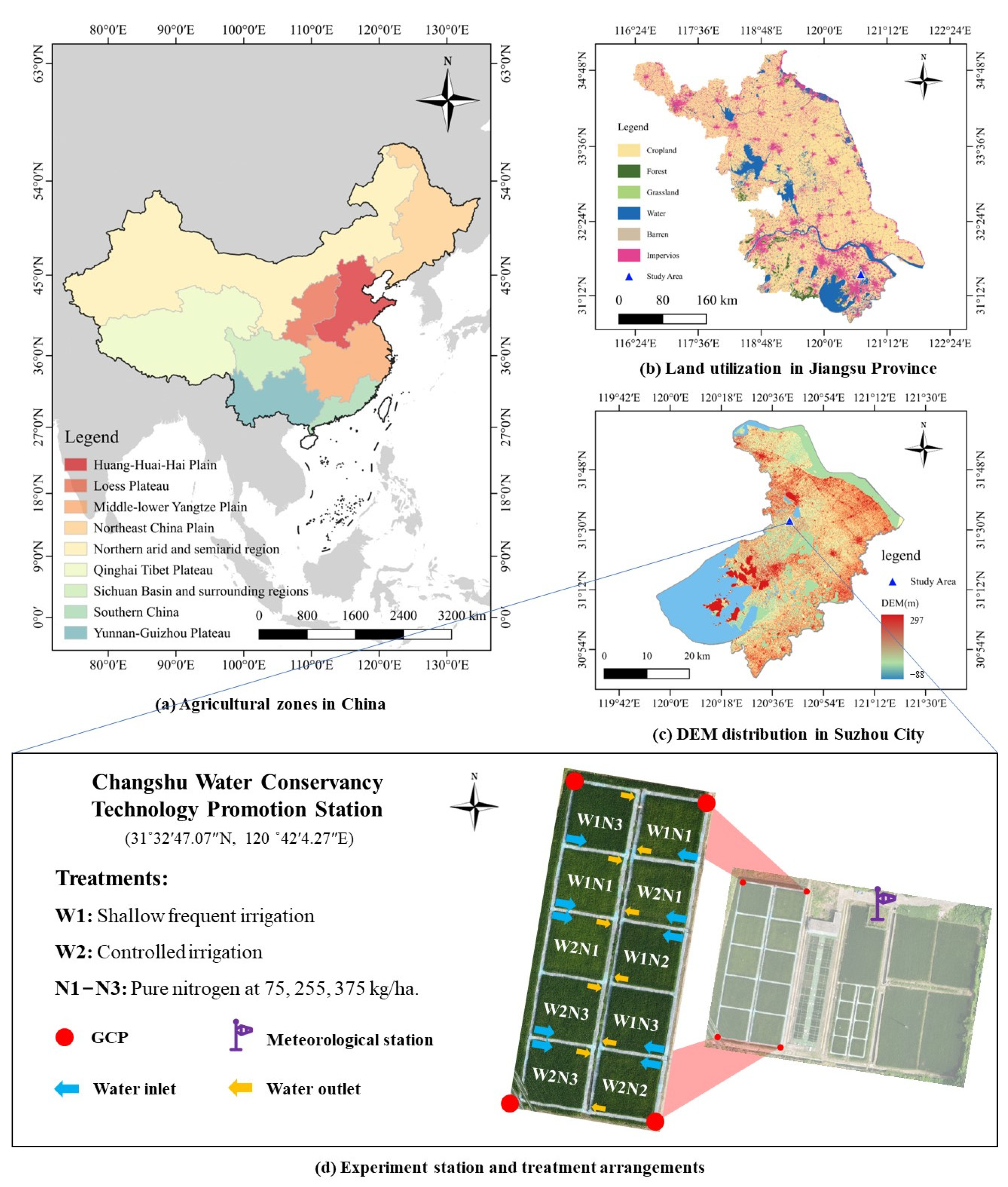
2.1. Study Area
2.2. Ground Data Measurements
2.2.1. Meteorological and Energy Flux Observations
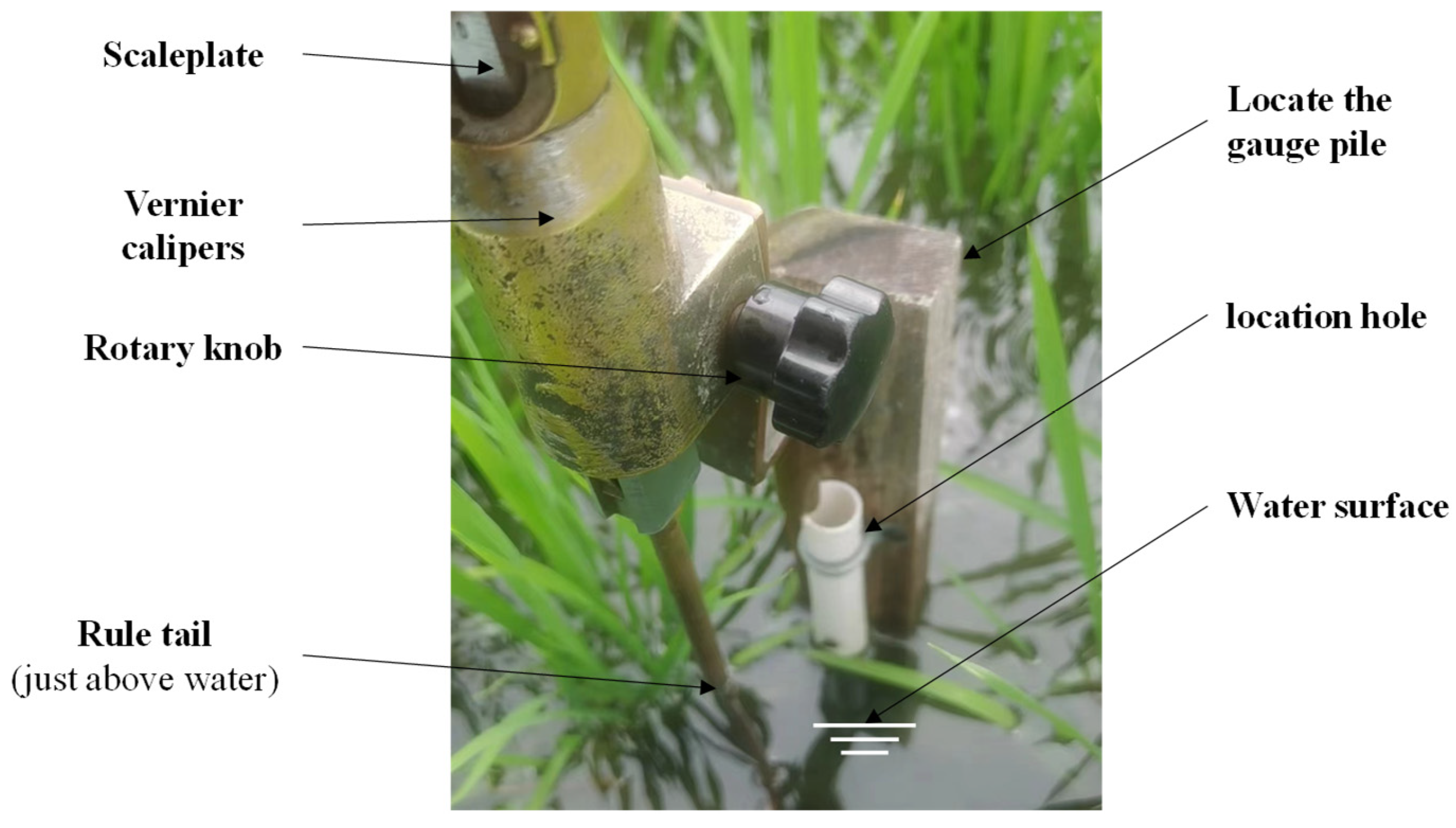
2.2.2. Field Scale ET Observations
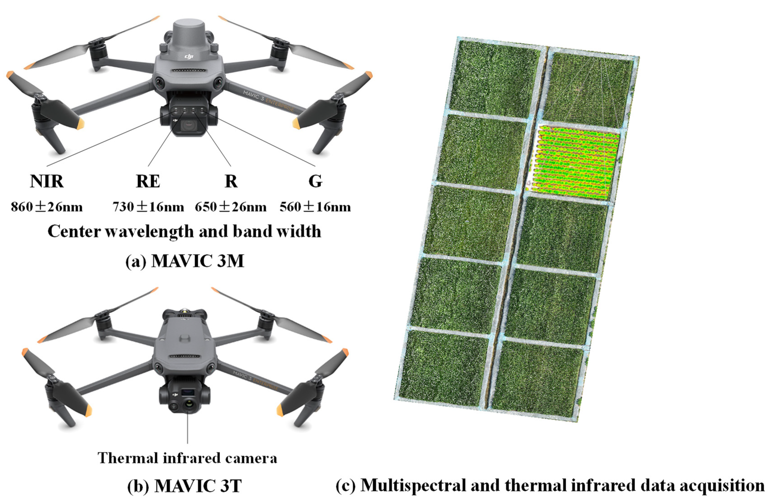
2.3. UAV-Based Data Acquisition and Processing
2.4. ET Estimation Methods
2.4.1. TSEB-PT
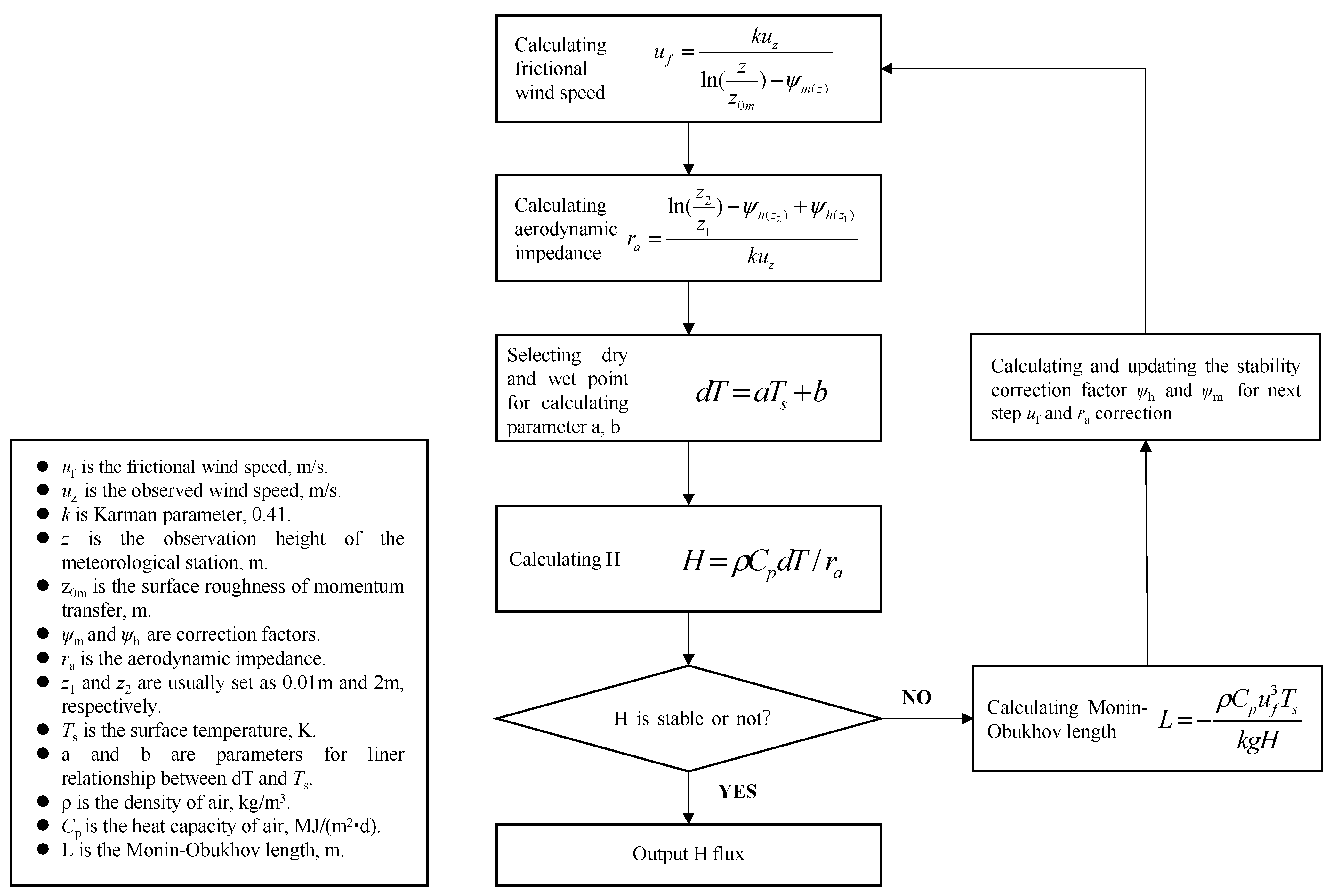
2.4.2. SEBAL
2.4.3. Single-Crop Coefficient Method
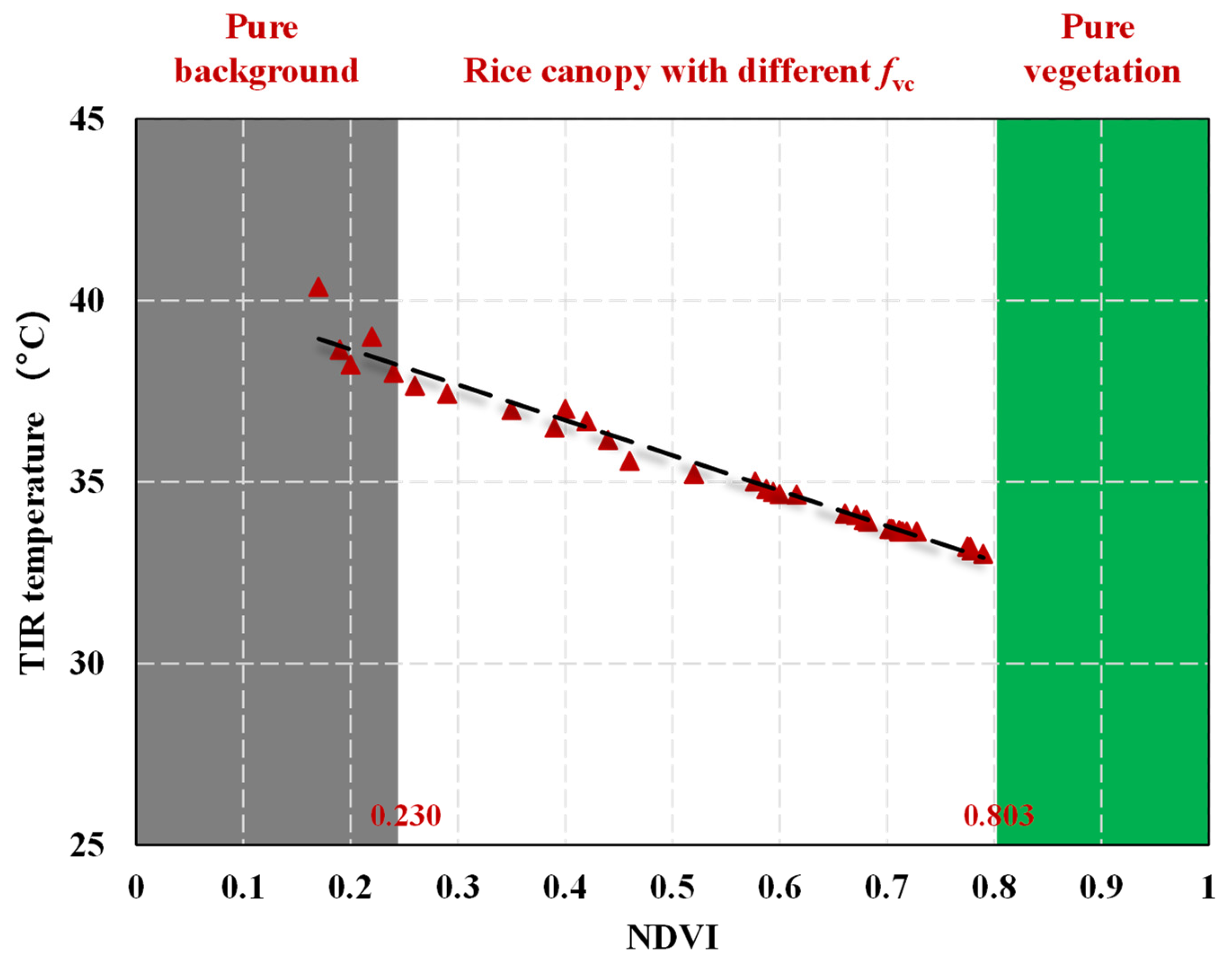
2.5. Calibration and Downscaling of Thermal Infrared Data
2.6. Evaluation Metrics
3. Results
3.1. Characteristics of Energy Distribution and ET in Rice Paddies
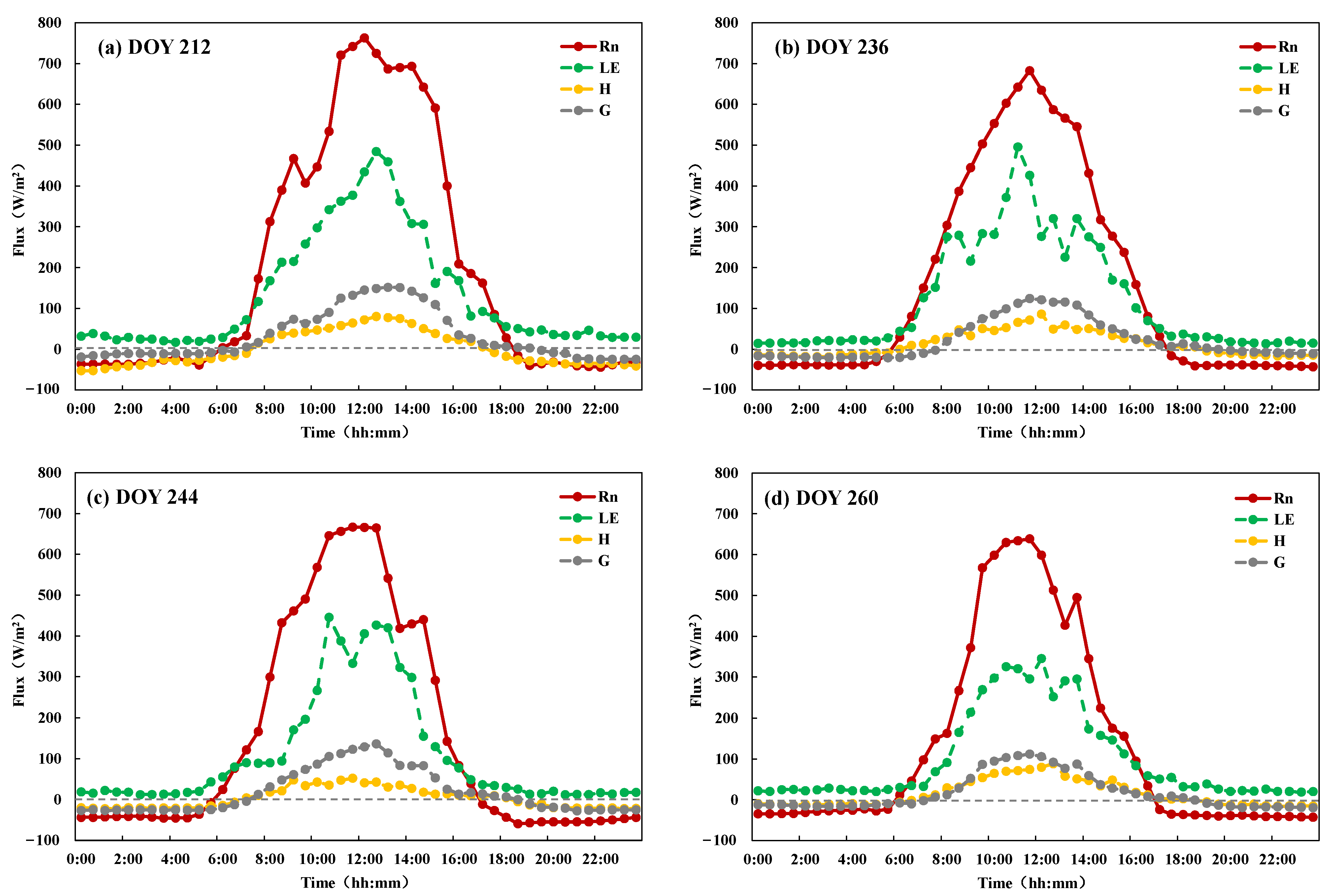
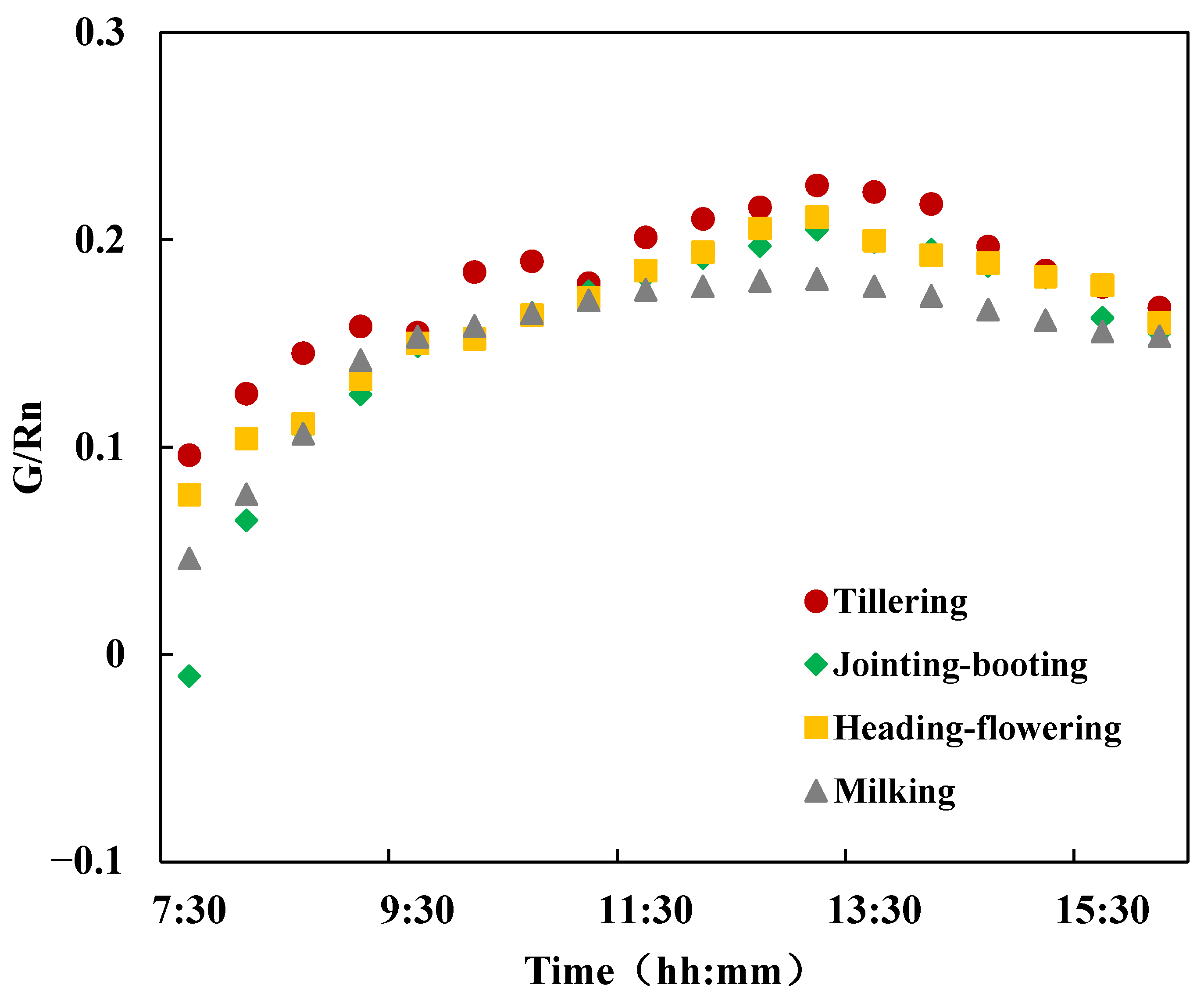
3.1.1. Energy Flux Diurnal Variation Under Typical Clear-Sky Conditions Across Growth Stages
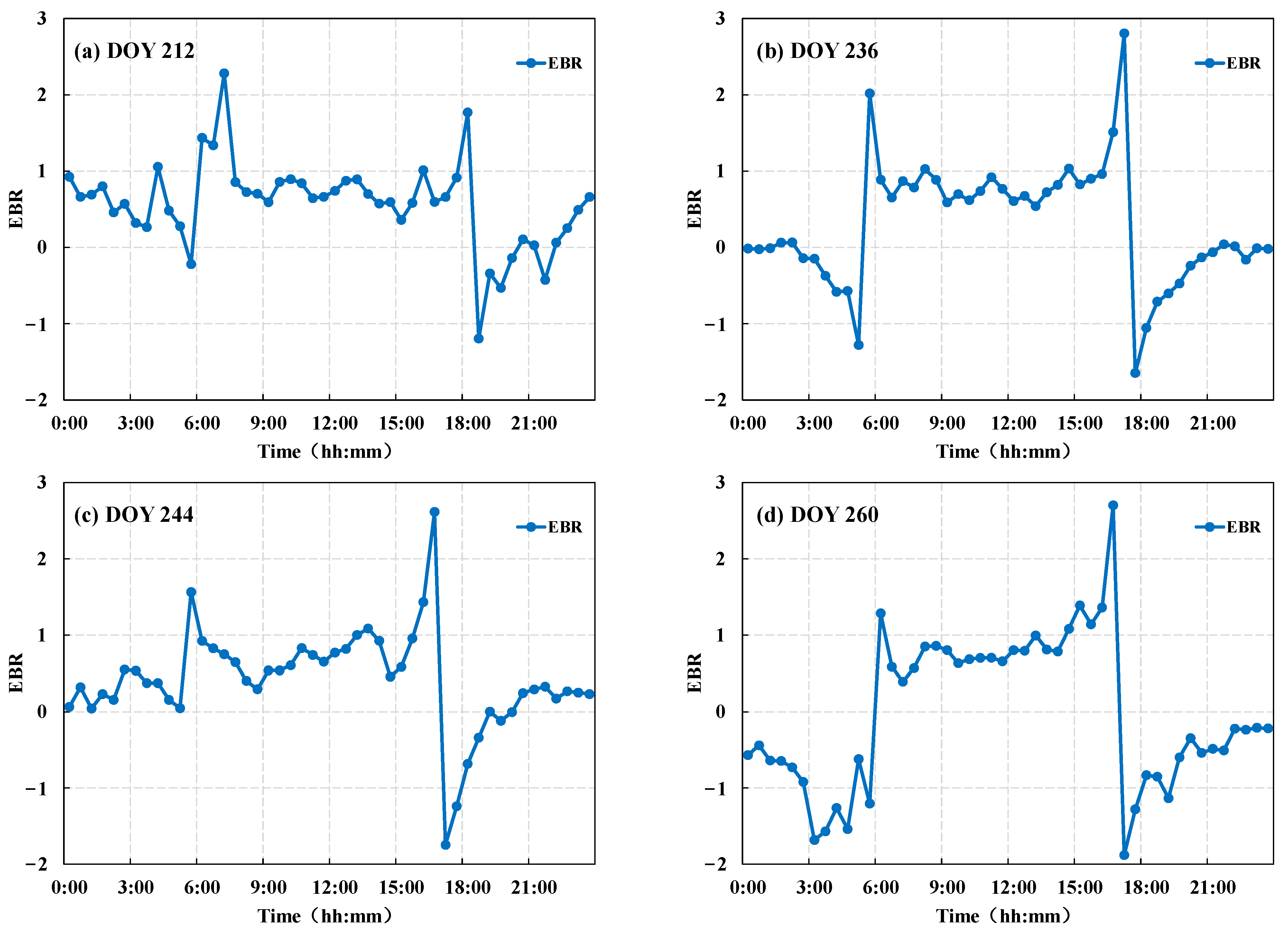
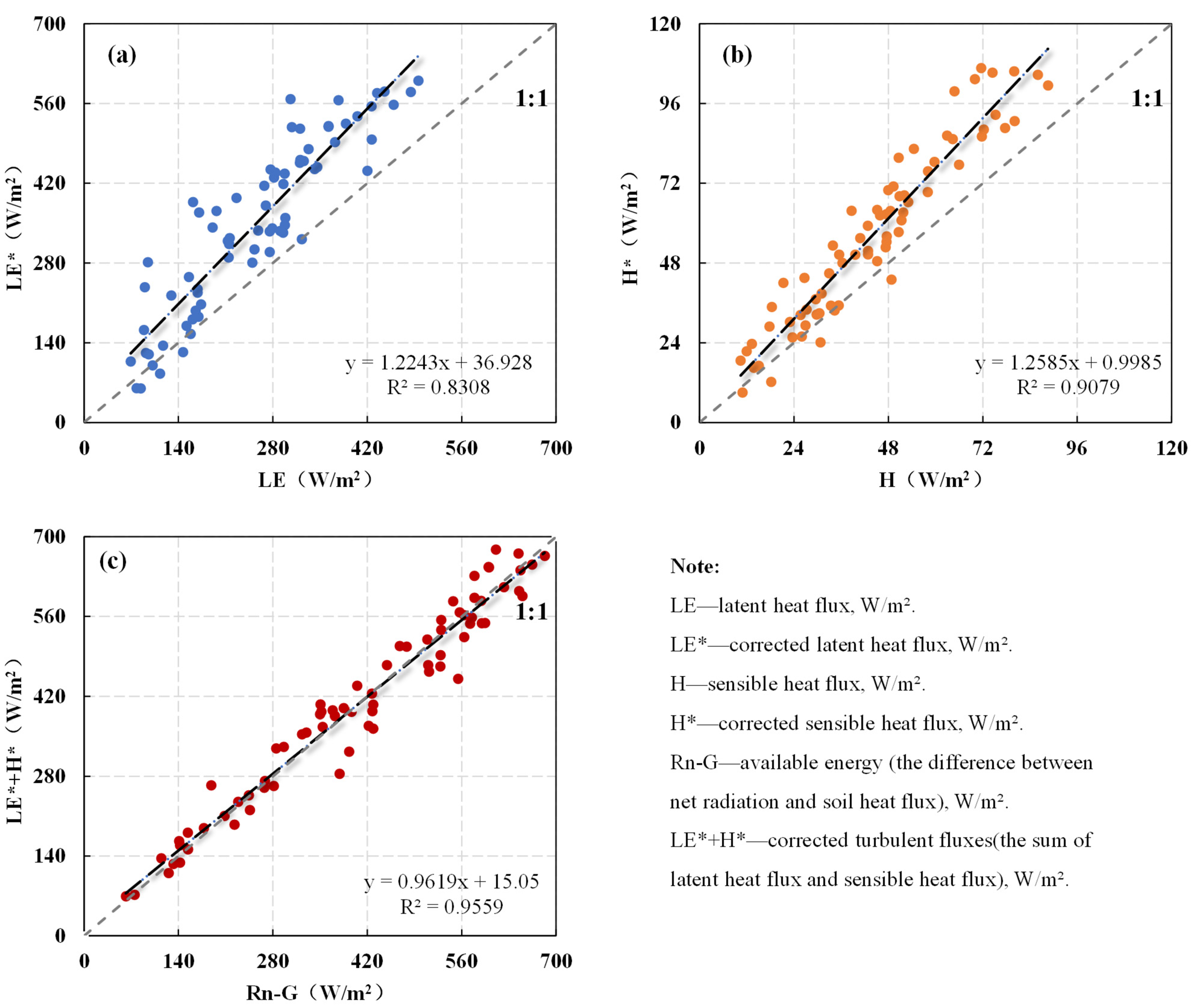
3.1.2. Energy Balance Characteristics and Enforcing Closure Correction
3.1.3. Field Scale ET Estimated Based on Flux Data and Single-Crop Coefficient Method
3.2. Effect of UAV Flight Strategy on Canopy Temperature Difference Identification Capability
3.2.1. Effect of Flight Altitudes on the Identification of Temperature Difference
3.2.2. Effect of Flight Times on the Identification of Temperature Difference
3.3. Evaluation of TSEB for ET Estimation in Rice Paddies
3.3.1. Adapting the TSEB Model Based on Prior Energy Flux Characteristics
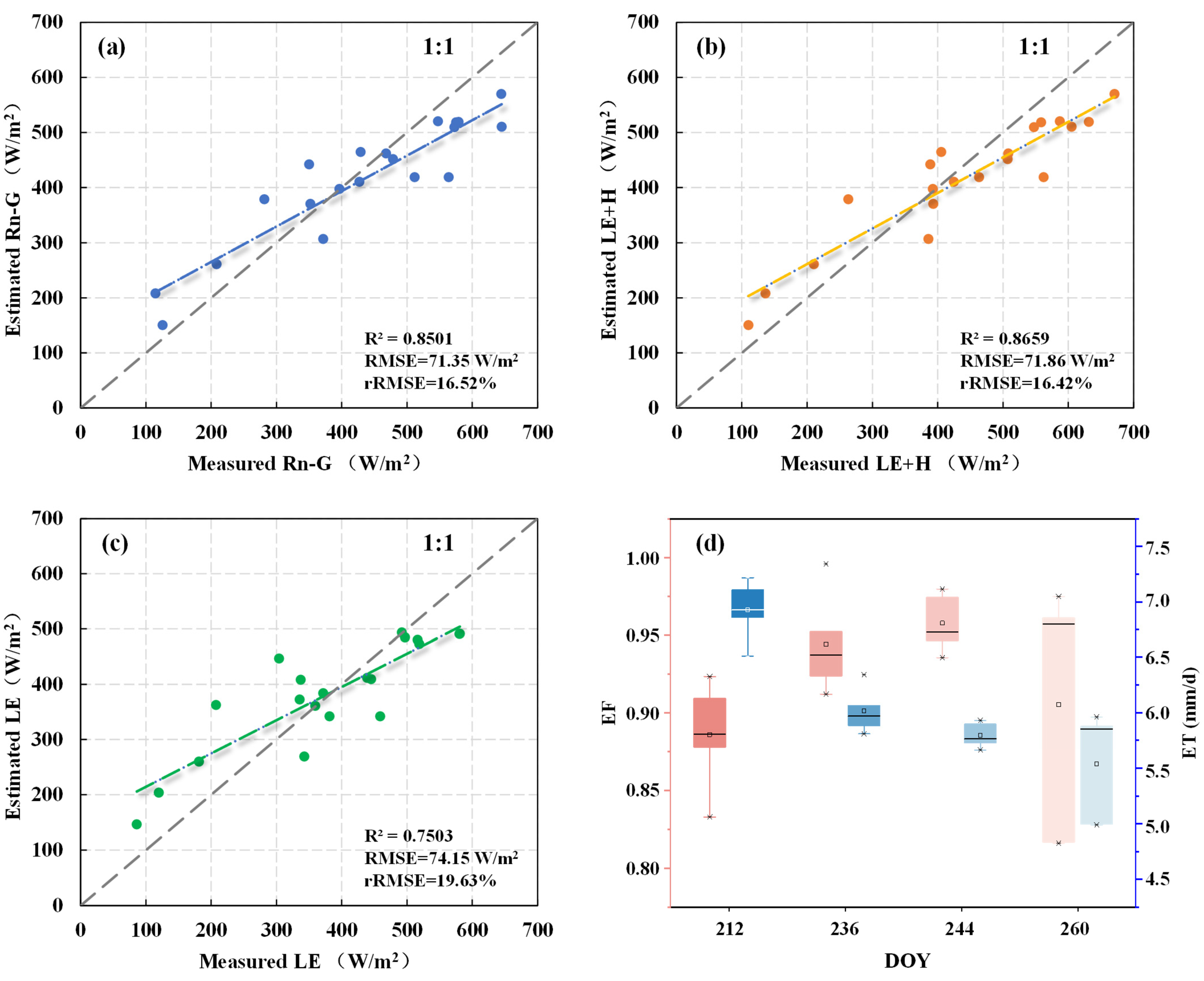
3.3.2. Energy Flux and ET Estimated Using the TSEB Model
4. Discussion
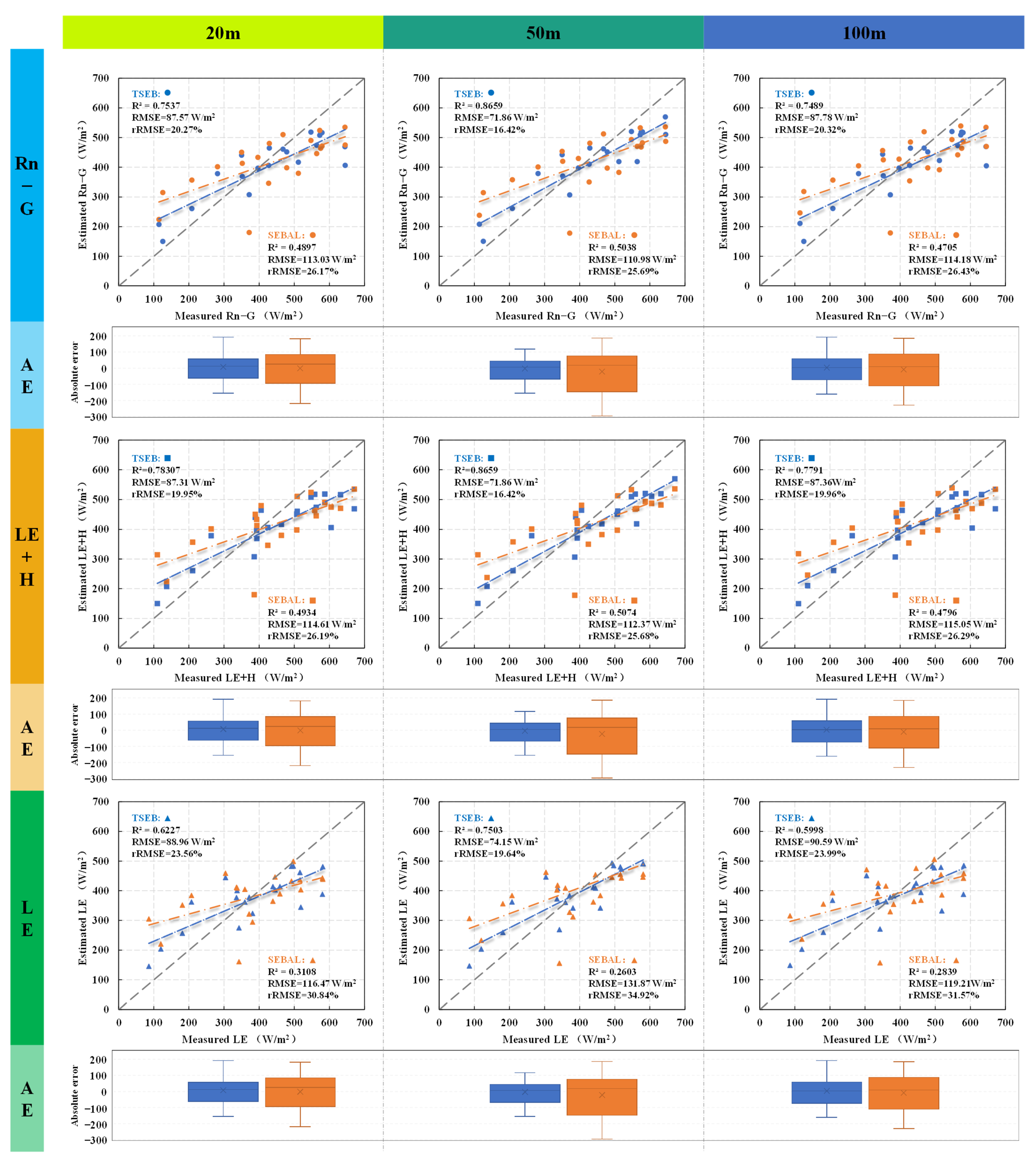
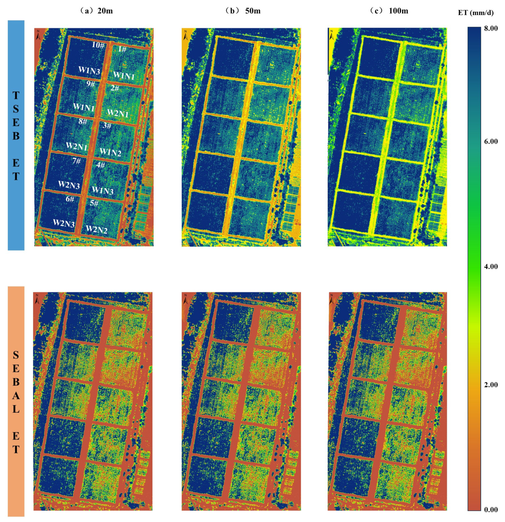
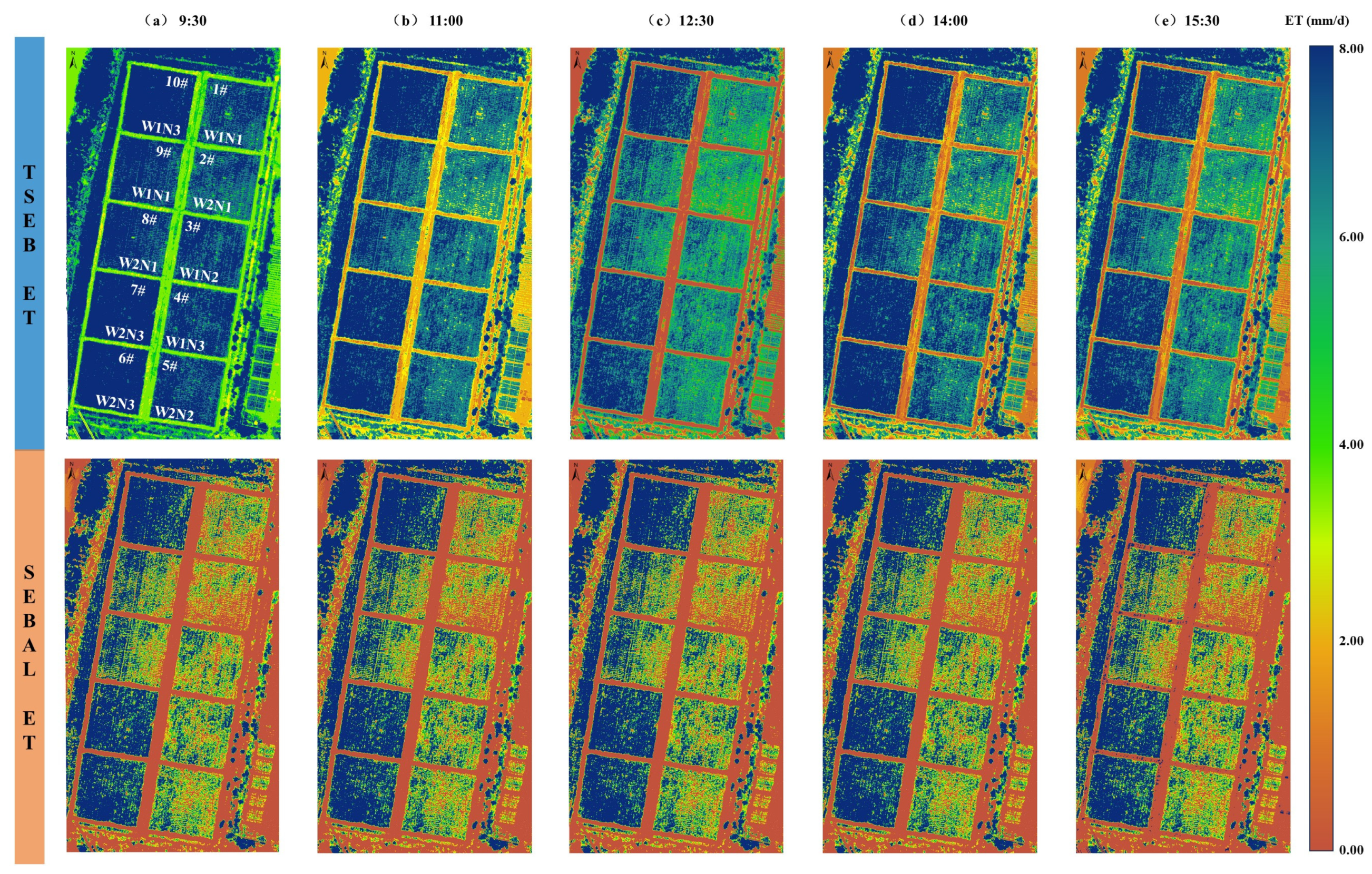
4.1. Accuracy Comparison of the TSEB and SEBAL Models on Energy Flux Estimation at Different Resolutions
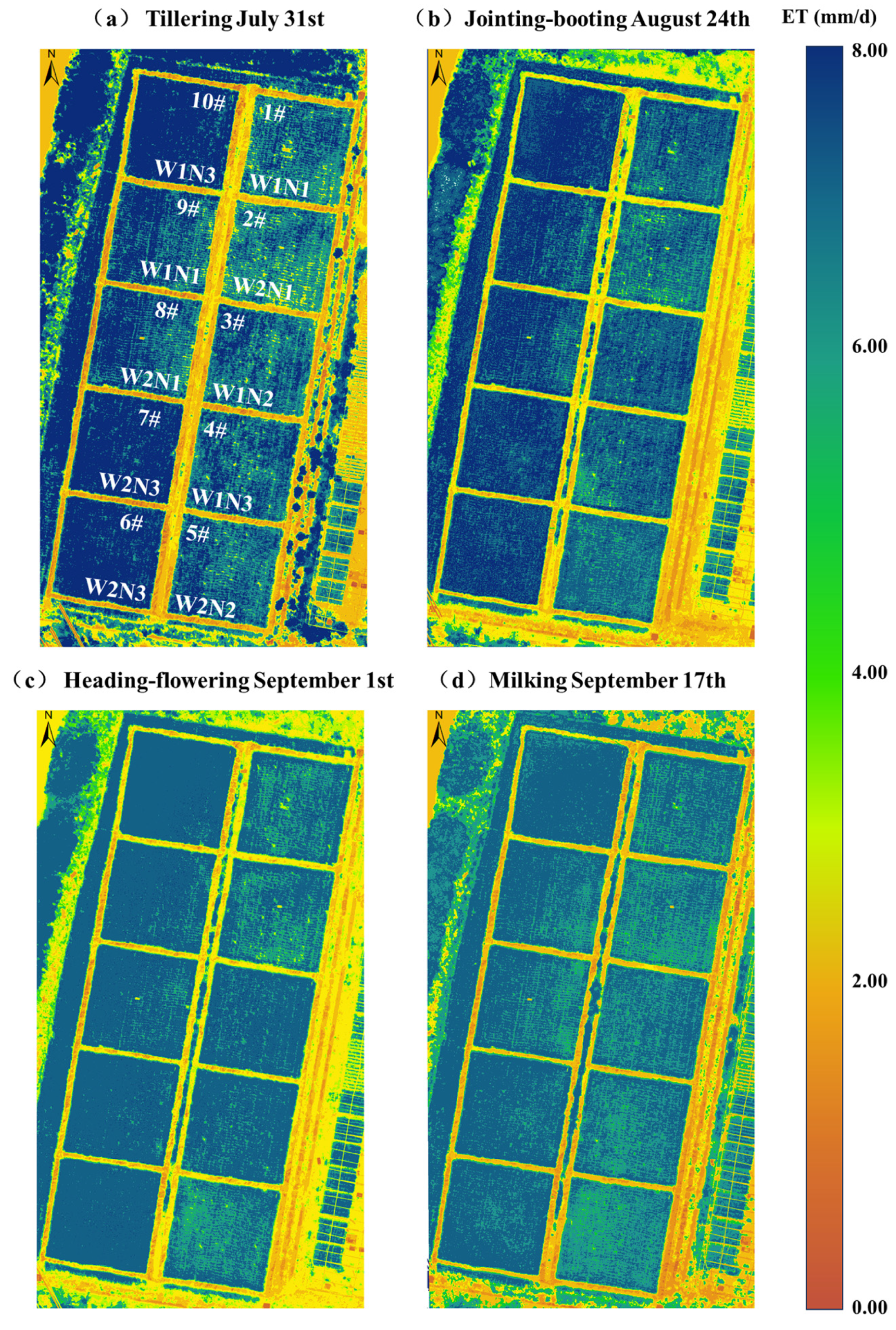
4.2. ET Assessment of Rice Paddies Under Different Treatments Based on the TSEB Model
5. Conclusions
- (1)
- The process of energy flux variation in rice paddies was dominated by Rn under typical clear-sky conditions with a single-peak diurnal pattern. The G/Rn ratio during the daytime can be accurately described by the constructed cosine diurnal variation model (R2 > 0.90), which effectively improved the fixed proportion calculation method of G in the original TSEB model.
- (2)
- The canopy TIR temperature gradually decreased with increasing altitudes but was consistently higher than the ground-measured values. Observations made at an altitude of 50 m at 11:00 am were more capable of effectively distinguishing temperature differences between treatments.
- (3)
- The TSEB model enabled the accurate simulation of energy flux and field scale ET in rice paddies, with R2 values of 0.8501 and 0.7503 for Rn − G and LE, respectively, with an absolute error ranging from −0.32 to −0.83 mm/d for ET. Comparisons with the SEBAL model further indicated that the TSEB model had a higher accuracy at different observation times and spatial resolutions.
Author Contributions
Funding
Data Availability Statement
Acknowledgments
Conflicts of Interest
References
- Frappart, F. Water and Life. Nat. Geosci. 2013, 6, 17. [Google Scholar] [CrossRef]
- Hunter, M.C.; Smith, R.G.; Schipanski, M.E.; Atwood, L.W.; Mortensen, D.A. Agriculture in 2050: Recalibrating Targets for Sustainable Intensification. Bioscience 2017, 67, 386–391. [Google Scholar] [CrossRef]
- Nesmith, A.A.; Schmitz, C.L.; Machado-Escudero, Y.; Billiot, S.; Forbes, R.A.; Powers, M.C.F.; Buckhoy, N.; Lawrence, L.A. Water, Air, and Land: The Foundation of Life, Food, and Society. In The Intersection of Environmental Justice, Climate Change, Community, and the Ecology of Life; Nesmith, A.A., Schmitz, C.L., Machado-Escudero, Y., Billiot, S., Forbes, R.A., Powers, M.C.F., Buckhoy, N., Lawrence, L.A., Eds.; Springer International Publishing: Cham, Switzerland, 2021; pp. 13–25. ISBN 978-3-030-55951-9. [Google Scholar]
- Irmak, S.; Kukal, M.S. Evapotranspiration, Transpiration, and Evaporation Processes and Modeling in the Soil–Residue–Canopy System. In Modeling Processes and Their Interactions in Cropping Systems; John Wiley & Sons, Ltd.: New York, NY, USA, 2022; pp. 53–114. ISBN 978-0-89118-386-0. [Google Scholar]
- Wu, T.; Zhang, W.; Jiao, X.; Guo, W.; Alhaj Hamoud, Y. Evaluation of Stacking and Blending Ensemble Learning Methods for Estimating Daily Reference Evapotranspiration. Comput. Electron. Agric. 2021, 184, 106039. [Google Scholar] [CrossRef]
- Yang, Y.; Roderick, M.L.; Guo, H.; Miralles, D.G.; Zhang, L.; Fatichi, S.; Luo, X.; Zhang, Y.; McVicar, T.R.; Tu, Z.; et al. Evapotranspiration on a Greening Earth. Nat. Rev. Earth Environ. 2023, 4, 626–641. [Google Scholar] [CrossRef]
- Pereira, L.S.; Allen, R.G.; Smith, M.; Raes, D. Crop Evapotranspiration Estimation with FAO56: Past and Future. Agric. Water Manag. 2015, 147, 4–20. [Google Scholar] [CrossRef]
- Wanniarachchi, S.; Sarukkalige, R. A Review on Evapotranspiration Estimation in Agricultural Water Management: Past, Present, and Future. Hydrology 2022, 9, 123. [Google Scholar] [CrossRef]
- Ghiat, I.; Mackey, H.R.; Al-Ansari, T. A Review of Evapotranspiration Measurement Models, Techniques and Methods for Open and Closed Agricultural Field Applications. Water 2021, 13, 2523. [Google Scholar] [CrossRef]
- Zhang, B.; Xu, D.; Liu, Y.; Chen, H. Review of multi-scale evapotranspiration estimation and spatio-temporal scale expansion. Trans. Chin. Soc. Agric. Eng. 2015, 31, 8–16. [Google Scholar]
- Liu, X.; Wang, G.; Yang, S.; Xu, J.; Wang, Y. Influence Factors and Characteristics of Transpiration and Evaporation in Water-Saving Irrigation Paddy Field under Different Temporal Scales. Trans. Chin. Soc. Agric. Mach. 2016, 47, 91–100, 170. [Google Scholar]
- Cellier, P.; Brunet, Y. Flux-Gradient Relationships above Tall Plant Canopies. Agric. For. Meteorol. 1992, 58, 93–117. [Google Scholar] [CrossRef]
- Dabberdt, W.; Lenschow, D.; Horst, T.; Zimmerman, P.; Oncley, S.; Delany, A. Atmosphere-Surface Exchange Measurements. Science 1993, 260, 1472–1481. [Google Scholar] [CrossRef] [PubMed]
- Allen, R.G.; Pereira, L.S.; Howell, T.A.; Jensen, M.E. Evapotranspiration Information Reporting: I. Factors Governing Measurement Accuracy. Agric. Water Manag. 2011, 98, 899–920. [Google Scholar] [CrossRef]
- Thunnissen, H.; Nieuwenhuis, G. An application of remote sensing and soil water balance simulation models to determine the effect of groundwater extraction on crop evapotranspiration. Agric. Water Manag. 1989, 15, 315–332. [Google Scholar] [CrossRef]
- Ray, S.; Dadhwal, V. Estimation of Crop Evapotranspiration of Irrigation Command Area Using Remote Sensing and GIS. Agric. Water Manag. 2001, 49, 239–249. [Google Scholar] [CrossRef]
- Dari, J.; Quintana-Seguí, P.; Morbidelli, R.; Saltalippi, C.; Flammini, A.; Giugliarelli, E.; Escorihuela, M.; Stefan, V.; Brocca, L. Irrigation Estimates from Space: Implementation of Different Approaches to Model the Evapotranspiration Contribution within a Soil-Moisture-Based Inversion Algorithm. Agric. Water Manag. 2022, 265, 107537. [Google Scholar] [CrossRef]
- Zhang, K.; Kimball, J.; Running, S. A Review of Remote Sensing Based Actual Evapotranspiration Estimation. Wiley Interdiscip. Rev. Water 2016, 3, 834–853. [Google Scholar] [CrossRef]
- Brown, K.; Rosenberg, N.J. A Resistance Model to Predict Evapotranspiration and Its Application to a Sugar Beet Field 1. Agron. J. 1973, 65, 341–347. [Google Scholar] [CrossRef]
- Liou, Y.; Kar, S. Evapotranspiration Estimation with Remote Sensing and Various Surface Energy Balance Algorithms-A Review. Energies 2014, 7, 2821–2849. [Google Scholar] [CrossRef]
- Segarra, J.; Buchaillot, M.; Araus, J.; Kefauver, S. Remote Sensing for Precision Agriculture: Sentinel-2 Improved Features and Applications. Agronomy 2020, 10, 641. [Google Scholar] [CrossRef]
- Wang, K.; Dickinson, R.E. A Review of Global Terrestrial Evapotranspiration: Observation, Modeling, Climatology, and Climatic Variability. Rev. Geophys. 2012, 50, RG2005. [Google Scholar] [CrossRef]
- Zhang, C.; Long, D.; Cui, Y.; Cui, Y.; Bai, L.; Dong, L. Applications of Remote Sensing Retrieval of Evapotranspiration in Irrigation Water Management: A Review. J. Hydraul. Eng. 2023, 54, 1087–1098. [Google Scholar]
- Bastiaanssen, W.G.M.; Pelgrum, H.; Wang, J.; Ma, Y.; Moreno, J.F.; Roerink, G.J.; van der Wal, T. A Remote Sensing Surface Energy Balance Algorithm for Land (SEBAL).: Part 2: Validation. J. Hydrol. 1998, 212–213, 213–229. [Google Scholar] [CrossRef]
- Bastiaanssen, W.G.; Molden, D.J.; Makin, I.W. Remote Sensing for Irrigated Agriculture: Examples from Research and Possible Applications. Agric. Water Manag. 2000, 46, 137–155. [Google Scholar] [CrossRef]
- Allen, R.G.; Tasumi, M.; Trezza, R. Satellite-Based Energy Balance for Mapping Evapotranspiration with Internalized Calibration (METRIC)—Model. J. Irrig. Drain. Eng. 2007, 133, 380–394. [Google Scholar] [CrossRef]
- Allen, R.; Irmak, A.; Trezza, R.; Hendrickx, J.; Bastiaanssen, W.; Kjaersgaard, J. Satellite-Based ET Estimation in Agriculture Using SEBAL and METRIC. Hydrol. Process. 2011, 25, 4011–4027. [Google Scholar] [CrossRef]
- Roerink, G.J.; Su, Z.; Menenti, M. S-SEBI: A Simple Remote Sensing Algorithm to Estimate the Surface Energy Balance. Phys. Chem. Earth Part B Hydrol. Ocean. Atmos. 2000, 25, 147–157. [Google Scholar] [CrossRef]
- Su, Z. The Surface Energy Balance System (SEBS) for Estimation of Turbulent Heat Fluxes. Hydrol. Earth Syst. Sci. 2002, 6, 85–100. [Google Scholar] [CrossRef]
- Norman, J.M.; Kustas, W.P.; Humes, K.S. Source Approach for Estimating Soil and Vegetation Energy Fluxes in Observations of Directional Radiometric Surface Temperature. Agric. For. Meteorol. 1995, 77, 263–293. [Google Scholar] [CrossRef]
- Shuttleworth, W.J.; Wallace, J. Evaporation from Sparse Crops-an Energy Combination Theory. Q. J. R. Meteorol. Soc. 1985, 111, 839–855. [Google Scholar] [CrossRef]
- Kato, T.; Kimura, R.; Kamichika, M. Estimation of Evapotranspiration, Transpiration Ratio and Water-Use Efficiency from a Sparse Canopy Using a Compartment Model. Agric. Water Manag. 2004, 65, 173–191. [Google Scholar] [CrossRef]
- Norman, J.M.; Kustas, W.P.; Prueger, J.H.; Diak, G.R. Surface Flux Estimation Using Radiometric Temperature: A Dual-Temperature-Difference Method to Minimize Measurement Errors. Water Resour. Res. 2000, 36, 2263–2274. [Google Scholar] [CrossRef]
- Song, L.; Kustas, W.P.; Liu, S.; Colaizzi, P.D.; Nieto, H.; Xu, Z.; Ma, Y.; Li, M.; Xu, T.; Agam, N.; et al. Applications of a Thermal-Based Two-Source Energy Balance Model Using Priestley-Taylor Approach for Surface Temperature Partitioning under Advective Conditions. J. Hydrol. 2016, 540, 574–587. [Google Scholar] [CrossRef]
- Song, L.; Ding, Z.; Kustas, W.P.; Xu, Y.; Zhao, G.; Liu, S.; Ma, M.; Xue, K.; Bai, Y.; Xu, Z. Applications of a Thermal-Based Two-Source Energy Balance Model Coupled to Surface Soil Moisture. Remote Sens. Environ. 2022, 271, 112923. [Google Scholar] [CrossRef]
- Evett, S.R.; Schwartz, R.C.; Howell, T.A.; Baumhardt, R.L.; Copeland, K.S. Can Weighing Lysimeter ET Represent Surrounding Field ET Well Enough to Test Flux Station Measurements of Daily and Sub-Daily ET? Adv. Water Resour. 2012, 50, 79–90. [Google Scholar] [CrossRef]
- Baldocchi, D. A Comparative Study of Mass and Energy Exchange Rates over a Closed C3 (Wheat) and an Open C4 (Corn) Crop: II. CO2 Exchange and Water Use Efficiency. Agric. For. Meteorol. 1994, 67, 291–321. [Google Scholar] [CrossRef]
- Baldocchi, D.; Falge, E.; Gu, L.; Olson, R.; Hollinger, D.; Running, S.; Anthoni, P.; Bernhofer, C.; Davis, K.; Evans, R.; et al. FLUXNET: A New Tool to Study the Temporal and Spatial Variability of Ecosystem-Scale Carbon Dioxide, Water Vapor, and Energy Flux Densities. Bull. Am. Meteorol. Soc. 2001, 82, 2415–2434. [Google Scholar] [CrossRef]
- Gentine, P.; Entekhabi, D.; Chehbouni, A.; Boulet, G.; Duchemin, B. Analysis of Evaporative Fraction Diurnal Behaviour. Agric. For. Meteorol. 2007, 143, 13–29. [Google Scholar] [CrossRef]
- Xu, T.; Liu, S.; Xu, L.; Chen, Y.; Jia, Z.; Xu, Z.; Nielson, J. Temporal Upscaling and Reconstruction of Thermal Remotely Sensed Instantaneous Evapotranspiration. Remote Sens. 2015, 7, 3400–3425. [Google Scholar] [CrossRef]
- Tang, R.; Li, Z. An Improved Constant Evaporative Fraction Method for Estimating Daily Evapotranspiration from Remotely Sensed Instantaneous Observations. Geophys. Res. Lett. 2017, 44, 2319–2326. [Google Scholar] [CrossRef]
- Wu, T.; Zhang, W.; Wu, S.; Cheng, M.; Qi, L.; Shao, G.; Jiao, X. Retrieving Rice (Oryza Sativa L.) Net Photosynthetic Rate from UAV Multispectral Images Based on Machine Learning Methods. Front. Plant Sci. 2023, 13, 1088499. [Google Scholar] [CrossRef]
- Kustas, W.; Norman, J. Evaluation of Soil and Vegetation Heat Flux Predictions Using a Simple Two-Source Model with Radiometric Temperatures for Partial Canopy Cover. Agric. For. Meteorol. 1999, 94, 13–29. [Google Scholar] [CrossRef]
- Guzinski, R.; Nieto, H.; Stisen, S.; Fensholt, R. Inter-Comparison of Energy Balance and Hydrological Models for Land Surface Energy Flux Estimation over a Whole River Catchment. Hydrol. Earth Syst. Sci. 2015, 19, 2017–2036. [Google Scholar] [CrossRef]
- Santanello, J.A.; Friedl, M.A. Diurnal Covariation in Soil Heat Flux and Net Radiation. J. Appl. Meteor. 2003, 42, 851–862. [Google Scholar] [CrossRef]
- Bastiaanssen, W. SEBAL-Based Sensible and Latent Heat Fluxes in the Irrigated Gediz Basin, Turkey. J. Hydrol. 2000, 229, 87–100. [Google Scholar] [CrossRef]
- Bastiaanssen, W.; Noordman, E.; Pelgrum, H.; Davids, G.; Thoreson, B.; Allen, R. SEBAL Model with Remotely Sensed Data to Improve Water-Resources Management under Actual Field Conditions. J. Irrig. Drain. Eng. 2005, 131, 85–93. [Google Scholar] [CrossRef]
- Grosso, C.; Manoli, G.; Martello, M.; Chemin, Y.; Pons, D.; Teatini, P.; Piccoli, I.; Morari, F. Mapping Maize Evapotranspiration at Field Scale Using SEBAL: A Comparison with the FAO Method and Soil-Plant Model Simulations. Remote Sens. 2018, 10, 1452. [Google Scholar] [CrossRef]
- Cheng, M.; Jiao, X.; Li, B.; Yu, X.; Shao, M.; Jin, X. Long Time Series of Daily Evapotranspiration in China Based on the SEBAL Model and Multisource Images and Validation. Earth Syst. Sci. Data 2021, 13, 3995–4017. [Google Scholar] [CrossRef]
- Pereira, L.; Paredes, P.; López-Urrea, R.; Hunsaker, D.; Mota, M.; Shad, Z.M. Standard Single and Basal Crop Coefficients for Vegetable Crops, an Update of FAO56 Crop Water Requirements Approach. Agric. Water Manag. 2021, 243, 106196. [Google Scholar] [CrossRef]
- Allen, R.G.; Pereira, L.S.; Raes, D.; Smith, M. Crop Evapotranspiration-Guidelines for Computing Crop Water Requirements-FAO Irrigation and Drainage Paper 56; Fao: Rome, Italy, 1998; Volume 300, p. D05109. [Google Scholar]
- Xu, J.; Peng, S.; Zhang, R.; Li, D. Neural Network Model for Reference Crop Evapotranspiration Prediction Based on Weather Forecast. J. Hydraul. Eng. 2006, 37, 376–379. [Google Scholar]
- Wang, W.; Peng, S.; Sun, F.; Xing, W.; Luo, Y.; Xu, J. Spatiotemporal Variations of Rice Irrigation Water Requirements in the Mid-Lower Reaches of Yangtze River under Changing Climate. Adv. Water Sci. 2012, 23, 656–664. [Google Scholar]
- Nieto, H.; Kustas, W.P.; Torres-Rúa, A.; Alfieri, J.G.; Gao, F.; Anderson, M.C.; White, W.A.; Song, L.; Alsina, M.D.M.; Prueger, J.H.; et al. Evaluation of TSEB Turbulent Fluxes Using Different Methods for the Retrieval of Soil and Canopy Component Temperatures from UAV Thermal and Multispectral Imagery. Irrig. Sci. 2019, 37, 389–406. [Google Scholar] [CrossRef] [PubMed]
- Gao, R.; Torres-Rua, A.F.; Nieto, H.; Zahn, E.; Hipps, L.; Kustas, W.P.; Alsina, M.M.; Bambach, N.; Castro, S.J.; Prueger, J.H.; et al. ET Partitioning Assessment Using the TSEB Model and sUAS Information across California Central Valley Vineyards. Remote Sens. 2023, 15, 756. [Google Scholar] [CrossRef]
- Peng, J.; Nieto, H.; Andersen, M.N.; Kørup, K.; Larsen, R.; Morel, J.; Parsons, D.; Zhou, Z.; Manevski, K. Accurate Estimates of Land Surface Energy Fluxes and Irrigation Requirements from UAV-Based Thermal and Multispectral Sensors. ISPRS J. Photogramm. Remote Sens. 2023, 198, 238–254. [Google Scholar] [CrossRef]
- Wei, J.; Cui, Y.; Luo, Y. Rice Growth Period Detection and Paddy Field Evapotranspiration Estimation Based on an Improved SEBAL Model: Considering the Applicable Conditions of the Advection Equation. Agric. Water Manag. 2023, 278, 108141. [Google Scholar] [CrossRef]
- Li, F.; Kustas, W.; Anderson, M.; Prueger, J.; Scott, R. Effect of Remote Sensing Spatial Resolution on Interpreting Tower-Based Flux Observations. Remote Sens. Environ. 2008, 112, 337–349. [Google Scholar] [CrossRef]
- Tao, S.; Song, L.; Zhao, G.; Zhao, L. Simulation and Assessment of Daily Evapotranspiration in the Heihe River Basin over a Long Time Series Based on TSEB-SM. Remote Sens. 2024, 16, 462. [Google Scholar] [CrossRef]
- Timmermans, W.J.; Kustas, W.P.; Anderson, M.C.; French, A.N. An Intercomparison of the Surface Energy Balance Algorithm for Land (SEBAL) and the Two-Source Energy Balance (TSEB) Modeling Schemes. Remote Sens. Environ. 2007, 108, 369–384. [Google Scholar] [CrossRef]
- Huete, A.; Didan, K.; Miura, T.; Rodriguez, E.P.; Gao, X.; Ferreira, L.G. Overview of the Radiometric and Biophysical Performance of the MODIS Vegetation Indices. Remote Sens. Environ. 2002, 83, 195–213. [Google Scholar] [CrossRef]
- Zeng, Y.; Hao, D.; Huete, A.; Dechant, B.; Berry, J.; Chen, J.M.; Joiner, J.; Frankenberg, C.; Bond-Lamberty, B.; Ryu, Y.; et al. Optical Vegetation Indices for Monitoring Terrestrial Ecosystems Globally. Nat. Rev. Earth Env. 2022, 3, 477–493. [Google Scholar] [CrossRef]


| Layer Depth (cm) | Clay (<2 μm) (%) | Powder (2–20 μm) (%) | Sand (2–2000 μm) (%) | Saturated Moisture Content (%) | Bulk Density (g/cm3) |
|---|---|---|---|---|---|
| 5–20 | 1.32 | 62.44 | 36.24 | 42.02 | 1.26 |
| 20–35 | 1.80 | 65.83 | 32.37 | 40.84 | 1.44 |
| 35–50 | 2.37 | 66.03 | 31.60 | 39.91 | 1.52 |
| Controlled Factors | Replanting | Tillering | Jointing–Booting | Heading–Flowering | Milking | Maturing |
|---|---|---|---|---|---|---|
| Shallow, frequent irrigation | ||||||
| Upper limit | 30 | 30 | 30 | 30 | 30 | 0 |
| Lower limit | 10 | 10 | 10 | 10 | 10 | 60%–70% * |
| Rain storage | 80 | 80~120 | 150–200 | 150–200 | 100 | 0 |
| Controlled irrigation | ||||||
| Upper limit | 100% * | 100% * | 100% * | 100% * | 100% * | 80% * |
| Lower limit | 10 | 80% * | 80% * | 80% * | 80% * | Drying |
| Rain storage | 70 | 80 | 100–150 | 100–150 | 80 | 0 |
| DOY | Time (hh:mm) | Solar Elevation Angle (°) | Flight Altitude (m) | Number of Images Obtained | Resolution (mm/pixel) |
|---|---|---|---|---|---|
| 212 | 09:30 | 52.98 | 20 50 100 | 576 (249) 204 (35) 56 (18) | 10 (30) 20 (70) 50 (140) |
| 11:00 | 70.45 | ||||
| 12:30 | 75.39 | ||||
| 14:00 | 60.53 | ||||
| 15:30 | 41.76 | ||||
| 236 | 09:30 | 50.00 | |||
| 11:00 | 65.38 | ||||
| 12:30 | 68.28 | ||||
| 14:00 | 55.36 | ||||
| 15:30 | 37.33 | ||||
| 244 | 09:30 | 48.92 | |||
| 11:00 | 63.33 | ||||
| 12:30 | 65.33 | ||||
| 14:00 | 52.83 | ||||
| 15:30 | 35.11 | ||||
| 260 | 09:30 | 45.80 | |||
| 11:00 | 58.34 | ||||
| 12:30 | 59.19 | ||||
| 14:00 | 47.64 | ||||
| 15:30 | 30.63 |
| Date | 31 July | 24 August | 1 September | 17 September | |
|---|---|---|---|---|---|
| DOY | 212 | 236 | 244 | 260 | |
| Rn | Peak Value | 762.90 | 682.50 | 666.70 | 638.50 |
| Peak Time | 12:00 | 12:00 | 11:30 | 11:30 | |
| Average | 194.64 | 157.18 | 149.66 | 129.53 | |
| H | Peak Value | 80.10 | 86.00 | 52.01 | 88.58 |
| Peak Time | 12:30 | 12:30 | 12:00 | 12:30 | |
| Average | 0.63 | 13.11 | 2.32 | 14.03 | |
| LE | Peak Value | 484.31 | 495.70 | 445.56 | 345.54 |
| Peak Time | 12:30 | 12:00 | 12:00 | 12:00 | |
| Average | 133.38 | 120.05 | 107.88 | 99.06 | |
| G | Peak Value | 151.76 | 124.27 | 136.52 | 112.20 |
| Peak Time | 13:00 | 13:00 | 13:00 | 13:00 | |
| Average | 31.03 | 22.02 | 17.69 | 16.95 | |
| DOY | Time | LE* (W/m2) | ETECh (mm/d) | ETEC (mm/d) | AEEC (mm/d) | ETKc (mm/d) | AEKc (mm/d) | ETm (mm/d) |
|---|---|---|---|---|---|---|---|---|
| 212 | 9:30 | 337.10 | 6.92 | 6.84 | −0.40 | 9.23 | 1.99 | 7.24 |
| 11:00 | 445.10 | 6.92 | ||||||
| 12:30 | 580.20 | 6.92 | ||||||
| 14:00 | 518.65 | 6.51 | ||||||
| 15:30 | 342.42 | 6.92 | ||||||
| 236 | 9:30 | 438.98 | 5.60 | 5.55 | −1.03 | 7.48 | 0.90 | 6.58 |
| 11:00 | 492.07 | 5.43 | ||||||
| 12:30 | 515.96 | 5.60 | ||||||
| 14:00 | 335.38 | 5.54 | ||||||
| 15:30 | 181.19 | 5.60 | ||||||
| 244 | 9:30 | 371.38 | 5.27 | 5.26 | −1.07 | 7.57 | 1.24 | 6.33 |
| 11:00 | 580.99 | 5.32 | ||||||
| 12:30 | 496.92 | 5.09 | ||||||
| 14:00 | 359.22 | 5.32 | ||||||
| 15:30 | 119.83 | 5.32 | ||||||
| 260 | 9:30 | 381.03 | 4.22 | 4.42 | −1.74 | 5.54 | −0.62 | 6.16 |
| 11:00 | 458.95 | 4.65 | ||||||
| 12:30 | 448.34 | 4.69 | ||||||
| 14:00 | 207.25 | 4.41 | ||||||
| 15:30 | 123.35 | 4.13 |
| Growth Stage | Altitude (m) | W1N1 | W1N2 | W1N3 | W2N1 | W2N2 | W2N3 |
|---|---|---|---|---|---|---|---|
| Tillering | 20 | 34.53 ± 0.54 abA | 34.14 ± 0.75 bcA | 33.41 ± 0.47 dA | 35.05 ± 0.96 aA | 33.61 ± 0.36 cdB | 33.23 ± 0.51 dA |
| 50 | 34.06 ± 0.41 bB | 33.58 ± 0.19 cB | 33.51 ± 0.30 cA | 34.59 ± 0.52 aAB | 34.50 ± 0.24 aA | 33.43 ± 0.30 cA | |
| 100 | 33.78 ± 0.43 aB | 32.78 ± 0.24 cC | 32.91 ± 0.44 bcB | 34.04 ± 0.74 aB | 33.26 ± 0.25 bC | 32.38 ± 0.26 dB | |
| Jointing–booting | 20 | 32.49 ± 1.10 aB | 31.33 ± 0.35 cA | 31.83 ± 0.52 abcA | 32.49 ± 0.49 aA | 32.14 ± 1.02 abA | 31.51 ± 0.25 bcA |
| 50 | 31.83 ± 0.56 abA | 30.53 ± 0.24 bcB | 30.68 ± 0.45 bcB | 31.57 ± 0.44 aB | 30.80 ± 0.24 bB | 30.43 ± 0.34 cC | |
| 100 | 31.36 ± 0.40 aA | 31.42 ± 0.52 bA | 31.43 ± 0.48 bA | 32.08 ± 0.70 aA | 31.59 ± 0.66 abA | 30.80 ± 0.32 dB | |
| Heading–flowering | 20 | 29.68 ± 1.36 abA | 28.93 ± 0.67 cdA | 27.68 ± 0.27 eA | 30.22 ± 0.55 aA | 29.29 ± 0.52 bcA | 28.37 ± 0.21 dB |
| 50 | 29.04 ± 0.76 bcA | 27.92 ± 0.23 dB | 27.79 ± 0.18 eA | 29.72 ± 0.50 aA | 29.11 ± 0.59 bA | 28.36 ± 0.16 cdB | |
| 100 | 28.72 ± 1.10 bcA | 28.71 ± 0.27 cA | 28.25 ± 0.24 dB | 29.73 ± 0.56 aA | 29.19 ± 0.52 bA | 28.63 ± 0.18 cdA | |
| Milking | 20 | 31.84 ± 0.24 aA | 31.24 ± 0.35 bA | 31.02 ± 0.12 bA | 31.65 ± 0.31 aA | 31.60 ± 0.57 aA | 31.07 ± 0.27 bA |
| 50 | 31.53 ± 0.22 aB | 30.78 ± 0.42 bB | 30.15 ± 0.30 cB | 31.17 ± 0.48 abB | 31.13 ± 0.76 abB | 30.23 ± 0.27 cB | |
| 100 | 30.99 ± 0.36 aC | 30.45 ± 0.37 bcB | 30.83 ± 0.55 abA | 30.81 ± 0.45 abB | 30.84 ± 0.48 abB | 30.27 ± 0.24 cB |
| Growth Stage | Time (hh:mm) | W1N1 | W1N2 | W1N3 | W2N1 | W2N2 | W2N3 |
|---|---|---|---|---|---|---|---|
| Tillering | 9:30 | 32.75 ± 0.36 aD | 31.66 ± 0.43 aD | 30.80 ± 0.19 cC | 32.61 ± 0.68 bD | 31.17 ± 0.25 cD | 31.76 ± 0.85 bD |
| 11:00 | 34.06 ± 0.41 bC | 33.58 ± 0.19 cC | 33.51 ± 0.30 cB | 34.59 ± 0.52 aC | 34.50 ± 0.24 aBC | 33.43 ± 0.30 cC | |
| 12:30 | 36.80 ± 0.77 abA | 35.82 ± 0.34 cA | 34.84 ± 0.36 dA | 37.29 ± 0.95 aA | 36.22 ± 0.70 bcA | 35.09 ± 0.53 dA | |
| 14:00 | 35.97 ± 0.98 aB | 34.87 ± 0.40 bB | 33.32 ± 0.30 cB | 35.64 ± 1.03 aB | 34.69 ± 0.52 bB | 33.91 ± 0.54 cBC | |
| 15:30 | 35.78 ± 0.93 aB | 34.90 ± 0.30 bB | 33.26 ± 0.20 dB | 35.12 ± 0.89 bBC | 34.27 ± 0.30 cC | 34.31 ± 0.24 cB | |
| Jointing–booting | 9:30 | 31.03 ± 0.46 bC | 30.15 ± 0.18 dD | 30.86 ± 0.85 bB | 31.63 ± 0.43 aC | 30.6 ± 0.23 bcD | 30.22 ± 0.18 cC |
| 11:00 | 31.36 ± 0.40 aC | 30.53 ± 0.24 bcC | 30.68 ± 0.45 bcC | 31.57 ± 0.44 aC | 30.80 ± 0.24 bD | 30.43 ± 0.34 cC | |
| 12:30 | 33.06 ± 0.90 bA | 31.26 ± 0.34 dB | 32.49 ± 1.22 bcA | 33.91 ± 1.02 aA | 32.07 ± 0.28 cB | 30.89 ± 0.29 dB | |
| 14:00 | 33.38 ± 0.70 bA | 31.65 ± 0.30 dA | 32.57 ± 0.92 cA | 34.01 ± 0.64 aA | 32.53 ± 0.16 cA | 31.40 ± 0.19 dA | |
| 15:30 | 32.27 ± 0.78 aB | 31.67 ± 0.16 bA | 31.53 ± 0.23 bB | 32.27 ± 0.40 aB | 31.78 ± 0.18 bC | 30.95 ± 0.26 cB | |
| Heading–flowering | 9:30 | 27.81 ± 0.91 bD | 26.75 ± 0.27 dE | 26.59 ± 0.18 dC | 28.47 ± 0.39 aD | 27.85 ± 0.71 bD | 27.61 ± 0.41 bD |
| 11:00 | 28.72 ± 1.10 bcBC | 27.92 ± 0.23 dC | 27.79 ± 0.18 eB | 29.72 ± 0.50 aC | 29.11 ± 0.59 bC | 28.36 ± 0.16 cdC | |
| 12:30 | 30.43 ± 1.05 cA | 29.37 ± 0.33 dA | 29.04 ± 0.25 dA | 31.99 ± 1.02 aA | 31.17 ± 0.98 bA | 30.38 ± 0.23 cA | |
| 14:00 | 29.09 ± 0.91 cB | 28.36 ± 0.15 dB | 27.71 ± 0.26 eB | 30.60 ± 0.76 aB | 29.99 ± 0.94 bB | 29.27 ± 0.30 cB | |
| 15:30 | 28.12 ± 0.66 bcC | 27.62 ± 0.18 cD | 26.92 ± 0.70 dC | 29.65 ± 0.50 aC | 29.16 ± 0.92 aC | 28.18 ± 0.21 bC | |
| Milking | 9:30 | 29.70 ± 0.20 aD | 29.32 ± 0.39 bD | 29.02 ± 0.21 dC | 29.58 ± 0.27 abD | 29.60 ± 0.49 abD | 29.53 ± 0.20 abD |
| 11:00 | 31.53 ± 0.22 aA | 30.78 ± 0.42 bA | 30.15 ± 0.30 cB | 31.17 ± 0.48 abAB | 31.13 ± 0.76 abA | 30.23 ± 0.27 cAB | |
| 12:30 | 31.77 ± 0.45 aA | 31.01 ± 0.26 bA | 30.59 ± 0.25 cA | 31.50 ± 0.53 aA | 31.04 ± 0.45 bAB | 30.36 ± 0.20 cA | |
| 14:00 | 31.17 ± 0.39 aB | 30.74 ± 0.13 bcA | 30.22 ± 0.31 dB | 31.04 ± 0.41 abB | 30.66 ± 0.18 cB | 29.84 ± 0.68 eC | |
| 15:30 | 30.70 ± 0.34 aC | 30.13 ± 0.46 cB | 30.02 ± 0.26 cB | 30.52 ± 0.33 abC | 30.26 ± 0.29 bcC | 30.00 ± 0.29 cBC |
| Growth Stage | DOY | (G/Rn)d | td | rRMSE (%) | R2 |
|---|---|---|---|---|---|
| Tillering | 212 | 0.22 | 13 | 5.55 | 0.9298 |
| Jointing–booting | 236 | 0.20 | 16.28 | 0.9368 | |
| Heading–flowering | 244 | 0.21 | 7.79 | 0.9767 | |
| Milking | 260 | 0.18 | 8.71 | 0.9215 |
| Treatment | Field ID | Tillering | Jointing–Booting | Heading–Flowering | Milking | ||||
|---|---|---|---|---|---|---|---|---|---|
| ETm | ETTSEB | ETm | ETTSEB | ETm | ETTSEB | ETm | ETTSEB | ||
| W1N1 | 1# | 6.98 | 6.79 | 6.49 | 6.02 | 6.22 | 5.65 | 5.88 | 4.97 |
| W1N1 | 9# | 7.04 | 6.86 | 6.35 | 6.09 | 6.31 | 5.81 | 5.72 | 5.12 |
| W1N2 | 3# | 7.24 | 6.93 | 6.58 | 6.06 | 6.33 | 5.73 | 6.16 | 4.99 |
| W1N3 | 4# | 7.27 | 6.99 | 6.66 | 6.03 | 6.48 | 5.72 | 6.55 | 5.33 |
| W1N3 | 10# | 8.21 | 7.66 | 6.85 | 6.28 | 6.62 | 5.88 | 6.48 | 5.54 |
| W2N1 | 2# | / | 6.59 | / | 5.92 | / | 5.61 | / | 4.98 |
| W2N1 | 8# | / | 6.73 | / | 5.87 | / | 5.78 | / | 5.18 |
| W2N2 | 5# | / | 6.85 | / | 5.93 | / | 5.57 | / | 4.98 |
| W2N3 | 6# | / | 7.54 | / | 6.24 | / | 5.63 | / | 5.17 |
| W2N3 | 7# | / | 7.55 | / | 6.21 | / | 5.71 | / | 5.25 |
Disclaimer/Publisher’s Note: The statements, opinions and data contained in all publications are solely those of the individual author(s) and contributor(s) and not of MDPI and/or the editor(s). MDPI and/or the editor(s) disclaim responsibility for any injury to people or property resulting from any ideas, methods, instructions or products referred to in the content. |
© 2025 by the authors. Licensee MDPI, Basel, Switzerland. This article is an open access article distributed under the terms and conditions of the Creative Commons Attribution (CC BY) license (https://creativecommons.org/licenses/by/4.0/).
Share and Cite
Wu, T.; Liu, K.; Cheng, M.; Gu, Z.; Guo, W.; Jiao, X. Paddy Field Scale Evapotranspiration Estimation Based on Two-Source Energy Balance Model with Energy Flux Constraints and UAV Multimodal Data. Remote Sens. 2025, 17, 1662. https://doi.org/10.3390/rs17101662
Wu T, Liu K, Cheng M, Gu Z, Guo W, Jiao X. Paddy Field Scale Evapotranspiration Estimation Based on Two-Source Energy Balance Model with Energy Flux Constraints and UAV Multimodal Data. Remote Sensing. 2025; 17(10):1662. https://doi.org/10.3390/rs17101662
Chicago/Turabian StyleWu, Tian’ao, Kaihua Liu, Minghan Cheng, Zhe Gu, Weihua Guo, and Xiyun Jiao. 2025. "Paddy Field Scale Evapotranspiration Estimation Based on Two-Source Energy Balance Model with Energy Flux Constraints and UAV Multimodal Data" Remote Sensing 17, no. 10: 1662. https://doi.org/10.3390/rs17101662
APA StyleWu, T., Liu, K., Cheng, M., Gu, Z., Guo, W., & Jiao, X. (2025). Paddy Field Scale Evapotranspiration Estimation Based on Two-Source Energy Balance Model with Energy Flux Constraints and UAV Multimodal Data. Remote Sensing, 17(10), 1662. https://doi.org/10.3390/rs17101662