Optimizing Data Consistency in UAV Multispectral Imaging for Radiometric Correction and Sensor Conversion Models

Abstract

Recent advancements in precision agriculture have been significantly bolstered by the Uncrewed Aerial Vehicles (UAVs) equipped with multispectral sensors. These systems are pivotal in transforming sensor-recorded Digital Number (DN) values into universal reflectance, crucial for ensuring data consistency irrespective of collection time, region, and illumination. This study, conducted across three regions in China using Sequoia and Phantom 4 Multispectral cameras, focused on examining the effects of radiometric correction on data consistency and accuracy, and developing a conversion model for data from these two sensors. Our findings revealed that radiometric correction substantially enhances data consistency in vegetated areas for both sensors, though its impact on non-vegetated areas is limited. Recalibrating reflectance for calibration plates significantly improved the consistency of band values and the accuracy of vegetation index calculations for both cameras. Decision tree and random forest models emerged as more effective for data conversion between the sensors, achieving R² values up to 0.91. Additionally, the P4M generally outperformed the Sequoia in accuracy, particularly with standard reflectance calibration. These insights emphasize the critical role of radiometric correction in UAV remote sensing for precision agriculture, underscoring the complexities of sensor data consistency and the potential for generalization of models across multi-sensor platforms.

1. Introduction

Owing to its cost-effectiveness and high efficiency, UAV technology has become increasingly prevalent in agricultural remote sensing [1,2,3,4]. UAVs, particularly those equipped with various optical sensors, are pivotal for tasks like classification, detection, and inversion, marking a new trend in contemporary research [5,6,7,8]. Predominantly, UAVs carry RGB and multispectral imaging systems, with the latter’s red edge and near-infrared reflectance being more extensively utilized in agriculture. Multispectral imaging, despite its larger bandwidths and discrete wavelengths that may lead to information loss compared to hyperspectral systems [9,10,11], offers advantages in terms of cost-effectiveness and ease of application [12,13]. Additionally, its compatibility with satellite remote sensing facilitates large-scale research validation [14]. Research has identified several key bands for vegetation, including green, red, red edge, and near-infrared, which are also the primary bands used in mainstream miniature multispectral sensors [15,16,17,18]. These bands suffice for most agricultural classification, detection, and inversion tasks.

The generalization ability of remote sensing models in agriculture is becoming increasingly crucial. The potential for correct model migration based on different multispectral imaging systems is a growing concern in current studies [6,19]. Data consistency refers to the uniformity of quantified results in the same area as captured by different sensors. In terms of the structure of mainstream multispectral imaging systems, which include a camera and a light sensor, the imaging band of the camera depends on its filter [20], leading to spectral information differences in the same band among various systems [21]. Moreover, the light sensor, used to capture real-time light intensity for each band and facilitate radiometric image correction, can vary in performance, affecting the correction outcome. These factors crucially influence data consistency across different multispectral imaging systems, impacting image model migration, particularly for inversion models reliant on spectral values [6,22,23].

Current research on sensor consistency has mainly focused on various satellite data types, with limited studies on miniature multispectral sensors’ data consistency [24,25,26]. While Lu et al. [21] investigated the consistency of the Parrot Sequoia and DJI Phantom 4 Multispectral cameras, concluding that data from these sensors can be converted through simple functions, their study lacked an in-depth discussion on how different ground features affect data consistency. Bueren et al. [27] highlighted the challenges and limitations in using optical UAV-based sensors over grasslands, emphasizing the necessity of thorough data acquisition and accurate calibration for reliable reflectance measurements. Studies by Zhao et al. [28] and Deng et al. [29] delved into UAV-based multispectral remote sensing’s potential in precision agriculture, discovering discrepancies between narrowband and broadband camera-derived data, complicating model generalization across devices.

The aim of this study is to assess how radiometric correction affects data consistency between two widely used UAV multispectral cameras—Parrot Sequoia and DJI Phantom 4 Multispectral—and to develop a sensor conversion model that enables data translation between them. By imaging the same agricultural sites with both sensors, we systematically evaluate the effect of different calibration approaches on sensor agreement and test whether a learned model can render their outputs interchangeable. The results offer practical guidance for multi-sensor data integration or sensor transitions in precision agriculture. For example, the proposed conversion model allows researchers to combine legacy data from Sequoia with newer P4M data in a unified analysis. Our work also compares sensor outputs against ground-based hyperspectral references and discusses the generalization potential of the conversion framework. The remainder of this paper is organized as follows: Section 2 introduces the study sites, data, and methods; Section 3 presents the results; Section 4 discusses the implications and limitations; and Section 5 concludes the work.

2. Materials and Methods

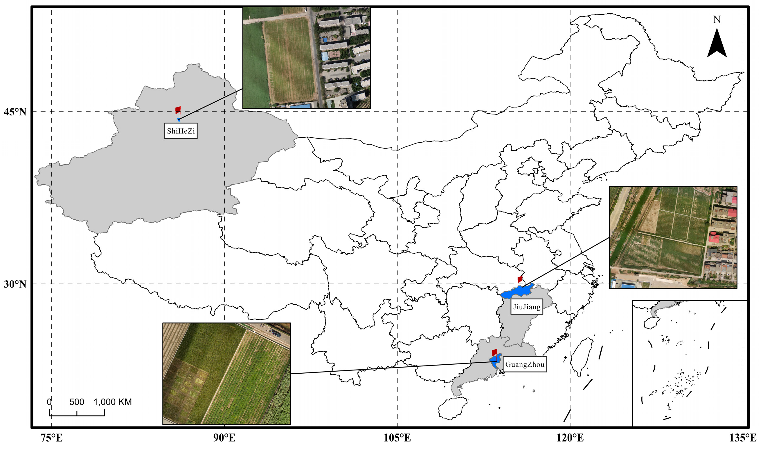
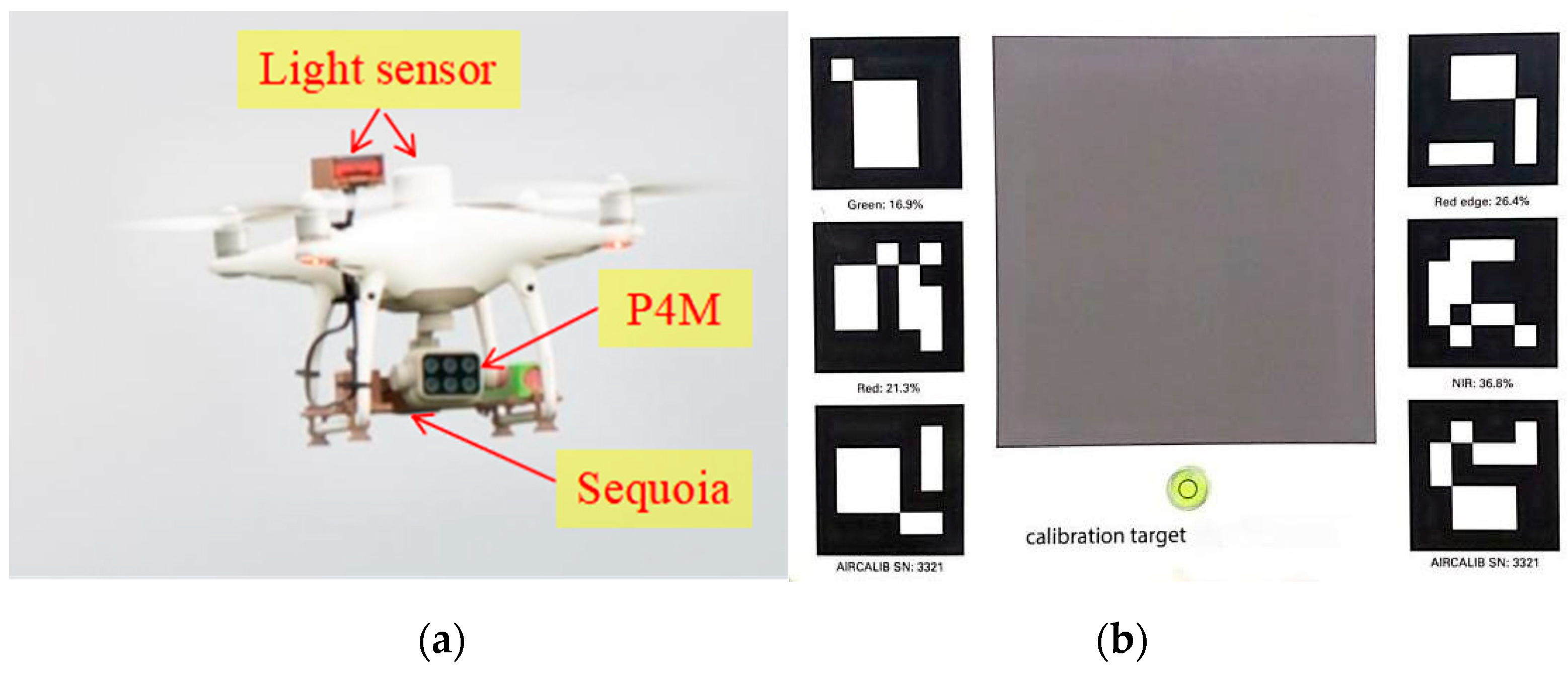
2.1. Study Area and Data Acquisition

In this experiment, multispectral images of various ground features were collected from three distinct regions of China: Shihezi City in Xinjiang (44.30°N, 86.00°E), Jiujiang City in Jiangxi Province (29.71°N, 115.83°E), and Guangzhou City in Guangdong Province (23.23°N, 113.63°E), as illustrated in Figure 1. These regions, extending over 20° in latitude, encompass diverse climates, including temperate continental and subtropical monsoon, and feature a wide array of ground objects, including both vegetated and non-vegetated areas. The imagery covers an area exceeding 230 hectares.

Shihezi City is located in a temperate continental climate zone, with agricultural land predominantly used for cotton and maize cultivation. The landscape also includes non-permeable surfaces and bare soil. Jiujiang City has a subtropical monsoon climate and features a mix of cotton, soybean, and rice fields. The area also contains urban infrastructure and non-permeable surfaces, providing a diverse mix of vegetated and non-vegetated areas. Guangzhou City, also located in a subtropical monsoon climate zone, includes agricultural fields of peanuts, maize, and rice, as well as urban areas with non-permeable surfaces like roads and buildings. Additionally, water bodies and scattered trees are present.

These regions were selected for their variety in vegetation types, urban and rural landscapes, and climatic conditions. The combination of agricultural areas, impervious surfaces, water bodies, and trees in these regions provides a comprehensive test environment for evaluating sensor calibration and radiometric correction methods, ensuring that the sensors are tested under diverse real-world conditions. Figure 2 depicts an overview of our study design and workflow.

For simultaneous remote sensing image acquisition, the Parrot Sequoia^® multispectral camera (Parrot, Paris, France) was affixed to a DJI Phantom 4 Multispectral (P4M) drone (DJI, Shenzhen, China) using a custom platform. While both cameras are equipped with light sensors, the Sequoia features four spectral bands, in contrast to the P4M’s five. Radiometric correction preparation for both sensors involved capturing images of correction plates (Figure 3). The wavelengths and bandwidths of the cameras are depicted in Figure 4, and the reflectance of the correction plates was measured with an ASD FieldSpec 4 Hi-Res spectroradiometer (Malvern Panalytical, Worcestershire, UK).

The planning and execution of the drone flights were facilitated by DJI GS Pro software (DJI, Version 2.0.17, Shenzhen, China) and conducted during noon for optimal lighting. The camera gimbal was set to a −90° angle, ensuring a 75% overlap rate between images. Each flight mission took about half an hour (

Table 1. Data acquisition parameters.

Location	Sensor	Date	Start Time of the Flight	Area Covered (ha)	Flight Altitude (M)	Ground Sample Distance (M/Pixel)
Shihezi	Sequoia	2 August 2022	12:00 a.m.	70	100	0.107
	P4M					0.056
Jiujiang	Sequoia	16 September 2022	11:00 a.m.	80		0.103
	P4M					0.054
	Sequoia	18 October 2022	11:00 a.m.	80		0.103
	P4M					0.054
Guangzhou	Sequoia	26 October 2022	11:30 a.m.	2	30	0.034
	P4M					0.017

). We selected ground sampling points in each experimental field to cover the diversity of ground cover types; most points were distributed in various types of vegetation. Figure 5 displays some of the typical types of sampling points. Hyperspectral reflectance data were gathered using the HandHeld2 ASD field spectrometer (Malvern Panalytical, Worcestershire, UK), with ten spectral curves obtained at each measurement point. The equipment, equipped with a 25° field-of-view foreoptic, positioned 35 cm above the ground and oriented towards the sun, covered a sampling area of 200 square centimeters. Whiteboard calibration was conducted using a Spectralon diffuse white reference panel (Malvern Panalytical, Worcestershire, UK) with a nominal reflectance of 0.999, supplied with the ASD HandHeld2 system. Calibration was performed at 15 min intervals or after changes in cloud cover, ensuring accurate correction of field-measured reflectance. In total, over ten types of ground objects and 80 sets of spectral reflectance data were gathered across the three regions. Each set of data contains 10 records, and the integration time for each record is 200 milliseconds. Each sampling point was geographically coordinated using Trimble Geo 7X (Trimble Navigation, Sunnyvale, CA, USA) in conjunction with the Qianxun Spatial Intelligence Inc. (Shanghai, China) network differential positioning service for real-time kinematic (RTK) surveying. With 5 to 10 records collected per positioning point at an accuracy of 1–2 cm, the geographic coordinates ensured consistency between ground features measured by the ASD and those captured by the UAV. These sampling points were used to validate UAV-derived reflectance values and serve as ground truth for evaluating the accuracy of vegetation indices and calibrating the sensor conversion models.

2.2. Radiometric Calibration Methodology

The multispectral images collected were initially processed using Pix4D mapper software (Pix4D, Version 4.4.12, Ecublens, Switzerland) for image stitching and radiometric correction. For the radiometric correction, we employed three approaches: The first method, standard correction (Stand), used the manufacturer-labeled reflectance values of the calibration plate [30]. However, over time, wear and tear on the calibration plate can lead to discrepancies between the standard and actual reflectance. The second method, ASD-based correction (ASD), involved recalibrating the plate’s reflectance using an ASD FieldSpec 4 under a tungsten halogen light source in a controlled indoor environment. The resulting reflectance spectrum was then converted into weighted average reflectance for each sensor’s spectral response (Figure 6). The relative spectral response (RSR) curves for the Sequoia and P4M multispectral sensors were obtained from the manufacturers. As the same reference panel was used in all field campaigns and remained in good condition, the recalibrated reflectance was applied across all experimental locations. The third method, uncorrected (DN), used the original digital number (DN) values without any radiometric correction. This process yielded two sets of orthophotos with corrected reflectance and one set with uncorrected DN values. Figure 7 illustrates the standard reflectance of the calibration plate and the weighted average reflectance for each sensor’s wavelength bands. Reflectance conversion follows the general Formula (1),

$${\mathrm{R}\mathrm{e}}_{\mathrm{t}}={\displaystyle \frac{{\mathrm{R}\mathrm{e}}_{\mathrm{p}}}{{\mathrm{D}\mathrm{N}}_{\mathrm{p}}}}\times {\mathrm{D}\mathrm{N}}_{\mathrm{t}}$$

(1)

where Re_t is the reflectance of the target, DN_t is the digital number of the target, DN_p is the DN of the panel, and Re_p is the reflectance of the panel (either standard or ASD-measured).

2.3. Image Pre-Processing

The P4M drone’s integration of RTK surveying via network differential positioning service facilitates high-precision geographic data acquisition without ground control points, achieving a positioning accuracy of 0.01–0.02 m. Consequently, the remote sensing images from P4M did not undergo geographic information correction. In contrast, the Sequoia sensor, relying on standard GPS positioning, incurs a positioning error exceeding 0.5 m. To rectify this, the Image Registration tool in ENVI software (Version 5.5, L3Harris, Melbourne, CA, USA, https://www.l3harris.com/ accessed on 5 June 2025) was utilized, aligning the Sequoia orthoimages with those from P4M through manual marking of homologous image points. Prior to registration, the Raster Resize tool was used to downsample the data for spatial resolution consistency, setting the Shihezi and Jiujiang data to 0.11 m/pixel and the Guangzhou data to 0.04 m/pixel.

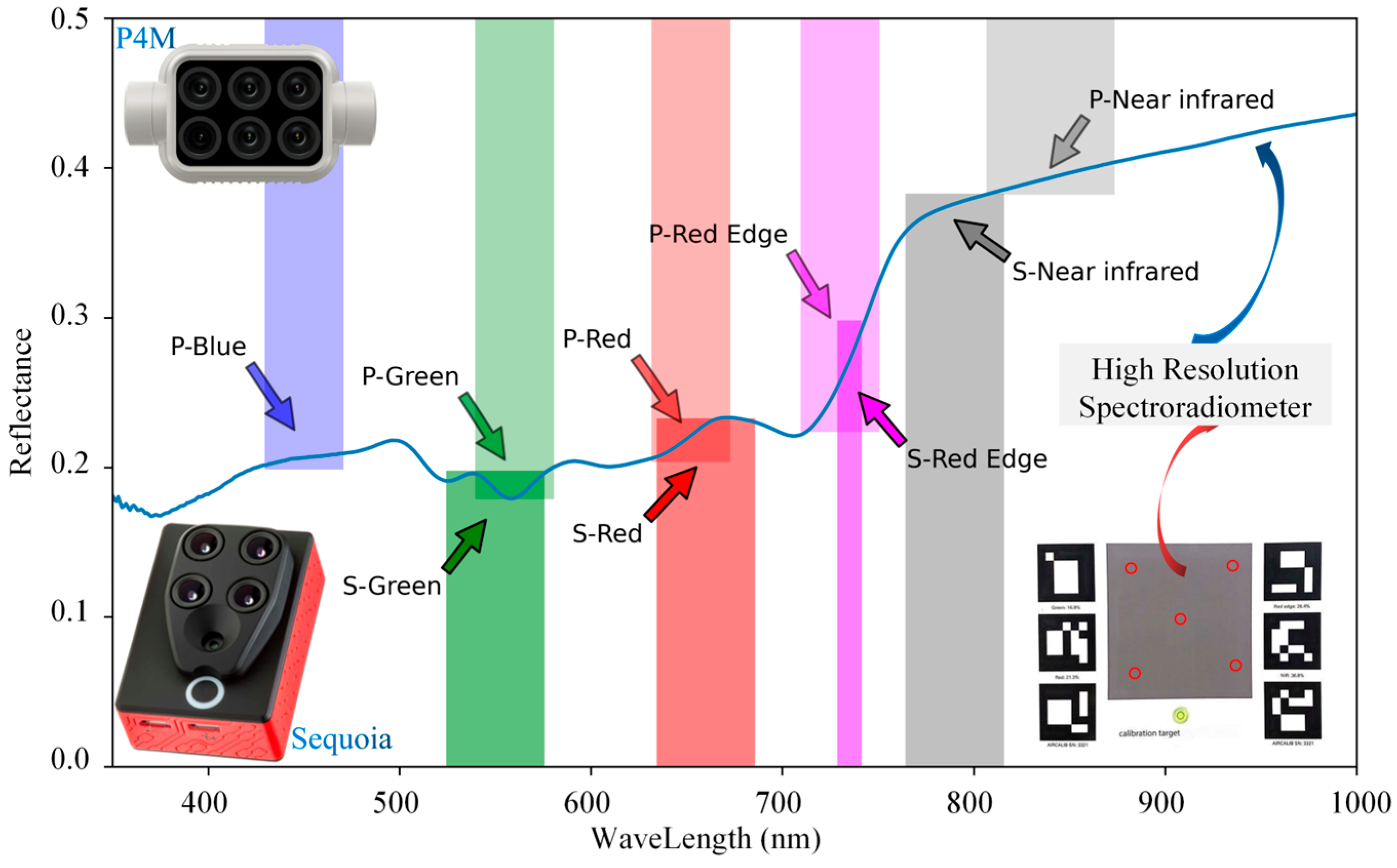
2.4. Spectral Reflectance Processing

Subsequent to exporting the hyperspectral data using ViewSpec software (Malvern Panalytical, Version 5.6, Worcestershire, UK), Python (Version 3.6) was employed to eliminate abnormal data appearing in multiple sampling records at each sampling point, ensuring data reliability. Abnormalities were detected using the Mahalanobis distance [31], as depicted in Figure 8. Differing from traditional Euclidean distance, which measures the distance between two points, Mahalanobis distance quantifies the distance between a point and a group, accounting for the group’s covariance matrix. The calculation process is shown in Formula (2).

$${\mathrm{D}}^2(\mathrm{A},\mathrm{G})={(\mathrm{A}-\mathsf{\mu })}^{\mathrm{T}}{\sum }^{-1}(\mathrm{A}-\mathsf{\mu })$$

(2)

Its formula involves sample point A, group G, group mean μ, and group covariance matrix $\sum$. A threshold of 1.5 was set to filter out spectral data with a Mahalanobis distance exceeding this value, achieving stable measurement results.

For each hyperspectral data sample, the average value was calculated from the spectral curves post-outlier removal. The average reflectance within the band ranges corresponding to the two sensors’ bands was then considered the measured spectral reflectance for those bands.

2.5. Image Reflectance and Vegetation Index Consistency Test Method

In this study, ten prevalent vegetation indices were calculated using images processed through three radiometric correction methods, with

Table 2. The vegetation indices used in this paper.

Vegetation Index Equation	Reference
Normalized Difference Vegetation Index $\mathrm{N}\mathrm{D}\mathrm{V}\mathrm{I}=(\mathrm{N}\mathrm{I}\mathrm{R}-\mathrm{R}\mathrm{E}\mathrm{D})/(\mathrm{N}\mathrm{I}\mathrm{R}+\mathrm{R}\mathrm{E}\mathrm{D})$	[32]
Ratio Vegetation Index $\mathrm{R}\mathrm{V}\mathrm{I}=\mathrm{N}\mathrm{I}\mathrm{R}/\mathrm{R}\mathrm{E}\mathrm{D}$	[33]
Difference Vegetation Index $\mathrm{D}\mathrm{V}\mathrm{I}=\mathrm{N}\mathrm{I}\mathrm{R}-\mathrm{R}\mathrm{E}\mathrm{D}$	[34]
Green Normalized Difference Vegetation Index $\mathrm{G}\mathrm{N}\mathrm{D}\mathrm{V}\mathrm{I}=(\mathrm{N}\mathrm{I}\mathrm{R}-\mathrm{G}\mathrm{R}\mathrm{E})/(\mathrm{N}\mathrm{I}\mathrm{R}+\mathrm{G}\mathrm{R}\mathrm{E})$	[35]
Modified Soil Adjusted Vegetation Index $\mathrm{M}\mathrm{S}\mathrm{A}\mathrm{V}\mathrm{I}=2\times \mathrm{N}\mathrm{I}\mathrm{R}+1-\sqrt{{(2\times \mathrm{N}\mathrm{I}\mathrm{R}+1)}^2-8(\mathrm{N}\mathrm{I}\mathrm{R}-\mathrm{R})}/2$	[36]
Green Chlorophyll Vegetation Index $\mathrm{G}\mathrm{C}\mathrm{V}\mathrm{I}=(\mathrm{N}\mathrm{I}\mathrm{R}/\mathrm{G}\mathrm{R}\mathrm{E})-1$	[37]
Red Edge Normalized Difference Vegetation Index $\mathrm{R}\mathrm{N}\mathrm{D}\mathrm{V}\mathrm{I}=(\mathrm{R}\mathrm{E}\mathrm{G}-\mathrm{R}\mathrm{E}\mathrm{D})/(\mathrm{R}\mathrm{E}\mathrm{G}+\mathrm{R}\mathrm{E}\mathrm{D})$	[37]
Normalized Difference Red Edge $\mathrm{N}\mathrm{D}\mathrm{R}\mathrm{E}=(\mathrm{N}\mathrm{I}\mathrm{R}-\mathrm{R}\mathrm{E}\mathrm{G})/(\mathrm{N}\mathrm{I}\mathrm{R}+\mathrm{R}\mathrm{E}\mathrm{G})$	[38]
Modified Red Edge Soil Adjusted Vegetation Index ${\mathrm{M}\mathrm{S}\mathrm{R}}_{\mathrm{r}\mathrm{e}}=(\mathrm{N}\mathrm{I}\mathrm{R}-\mathrm{R}\mathrm{E}\mathrm{G}-1)/(\sqrt{\mathrm{N}\mathrm{I}\mathrm{R}-\mathrm{R}\mathrm{E}\mathrm{G}}+1)$	[39]
Red Edge Chlorophyll Vegetation Index ${\mathrm{C}\mathrm{L}}_{\mathrm{r}\mathrm{e}}=(\mathrm{N}\mathrm{I}\mathrm{R}/\mathrm{R}\mathrm{E}\mathrm{G})-1$	[40]

delineating the calculation method for each index. To evaluate the correlation between images corrected by different methods, the Pearson correlation coefficient was computed using ENVI’s raster tool. Standard reflectance refers to the reflectance marked on the calibration plate by the manufacturer, while re-measured reflectance refers to the reflectance values measured from the calibration plates by an ASD, which were used for radiometric calibration of the sensor data.

Furthermore, correlation functions were developed using Python (version 3.6) to generate 16,000 random points per image. A series of concentric circle buffers (0, 0.2, 0.5, 1.0, and 1.5 m in diameter) were created around each point. The average reflectance for each band at each point and for each correction phase was extracted using Python’s rasterio library. These reflectance values were then correlated using the Pearson coefficient (Formula (3)), a statistical measure commonly used to assess the linear correlation between two data sets, X and Y.

Given the NDVI’s limited dynamic range, which amplifies differences in non-vegetated areas between sensors, the Root Mean Square Error (RMSE) was employed for a more nuanced evaluation of inter-sensor differences (Formula (4)). The NRMSE (Formula (5)), considering the dimensionality of the variable, was utilized to enable comprehensive comparisons between the bands and vegetation indices from different sensors.

$$\mathrm{C}\mathrm{O}\mathrm{R}(\mathrm{X},\mathrm{Y})={\displaystyle \frac{{\sum }_{\mathrm{i}}^{\mathrm{n}}({\mathrm{X}}_{\mathrm{i}}-\overline{\mathrm{X}})({\mathrm{Y}}_{\mathrm{i}}-\overline{\mathrm{Y}})}{\sqrt{{\sum }_{\mathrm{i}}^{\mathrm{n}}{({\mathrm{X}}_{\mathrm{i}}-\overline{\mathrm{X}})}^2{\sum }_{\mathrm{i}}^{\mathrm{n}}{({\mathrm{Y}}_{\mathrm{i}}-\overline{\mathrm{Y}})}^2}}}$$

(3)

$$\mathrm{R}\mathrm{M}\mathrm{S}\mathrm{E}=\sqrt{{\displaystyle \frac{1}{\mathrm{n}}}{\sum }_{\mathrm{i}=1}^{\mathrm{n}}{({\mathrm{X}}_{\mathrm{i}}-{\mathrm{Y}}_{\mathrm{i}})}^2}$$

(4)

$$\mathrm{N}\mathrm{R}\mathrm{M}\mathrm{S}\mathrm{E}={\displaystyle \frac{\mathrm{R}\mathrm{M}\mathrm{S}\mathrm{E}}{\overline{\mathrm{Y}}}}\times 100\mathrm{\%}$$

(5)

In the formula, X and Y represent two groups of variables, $\overline{\mathrm{X}}$ and $\overline{\mathrm{Y}}$ represent the means of these groups, respectively, and n represents the total number of samples.

2.6. Evaluation Method of Spectral Data and Vegetation Index Accuracy

In this study, 80 sets of manually collected hyperspectral reflectance data, paired with corresponding positioning information, were integrated. Average band values were extracted from the three types of spectral images (Stand, ASD, and DN) across the various buffer zones. These values were then paired with the hyperspectral data to form data pairs. The spectral reflectance of actual ground objects within the corresponding bands was calculated using the weighted average hyperspectral reflectance within those bands. Subsequently, canonical vegetation index values were derived from the spectral data pairs. The spectral data’s accuracy was assessed using the coefficient of determination (R², Formula (6)) and the RMSE, as calculated by the following formulas:

$${\mathrm{R}}^2={\displaystyle \frac{{\mathrm{S}\mathrm{S}}_{\mathrm{R}}}{{\mathrm{S}\mathrm{S}}_{\mathrm{T}}}}={\displaystyle \frac{\sum {(\widehat{{\mathrm{X}}_{\mathrm{i}}}-\overline{\mathrm{Y}})}^2}{\sum {({\mathrm{Y}}_{\mathrm{i}}-\overline{\mathrm{Y}})}^2}}$$

(6)

In these formulas, SS_R represents the residual sum of squares, SS_T represents the total sum of squares, X represents values derived from multispectral imagery, and Y denotes values from hyperspectral data.

2.7. Conversion Model and Feature Importance Analysis

This study also tested five common fitting methods to construct a conversion model between the two sensors, aimed at enhancing the accuracy of image data. Utilizing the scikit-learn library (version 0.24) in Python (version 3.6), linear regression, decision tree regression, random forest regression, support vector machine regression, and polynomial regression models were constructed. Except for the third-order polynomial, default parameters were applied to all models.

Through evaluations of consistency and accuracy, the model selected the sensor with higher accuracy as the conversion target, and the radiometric correction method and buffer size demonstrating the best consistency and accuracy as the data source for modeling. Data pairs were filtered to create a dataset for each band, divided into training and test sets (80:20 ratio). Model accuracy was evaluated using R² and RMSE.

3. Results

3.1. Consistency Analysis of Image Data

The correlation analysis of the four bands in this study revealed varying degrees of correlation between the two sensors, contingent on the type of ground objects and the radiometric correction methods employed. Figure 9 presents the Pearson correlation between corresponding reflectance images from the P4M and Sequoia sensors, evaluated under three different radiometric calibration conditions (standard reflectance, re-measured/ASD reflectance, and uncorrected DN). The left section of the figure displays RGB images and the pseudo-color maps of Pearson coefficients under different radiometric correction methods. These colors, determined by the corresponding Pearson coefficients, are used to spatially assess the coefficient distribution. The upper right section shows histograms of the pseudo-color images, aiding in evaluating the Pearson coefficient distributions between sensors under various correction methods, with insets focusing on specific values at −1, 0, and 1. The lower right section highlights representative details of these enlargements, revealing distinct correlations in reflectance images derived from different correction methods. Notably, most pixel correlations post-correction were above 0.97 (median > 0.97), while correlations without correction predominantly exceeded 0.75 (median between 0.75 and 0.9).

The figure also demonstrates that high correlations in radiometrically corrected images between sensors were mainly evident in vegetated ground surfaces (dark blue areas in Figure 9). In contrast, artificial structures, shadows, and bare soil frequently exhibited negative correlations (dark red areas), while some roads and water bodies showed poor correlation (light areas). For non-corrected images, vegetation maintained high correlation, but other ground object types lacked consistent patterns.

3.2. Consistency Test of Each Band Value and Vegetation Index

Over 500,000 data pairs were collected from the three image types (Stand, ASD, and DN) by randomly placing sampling points of various sizes. The Pearson coefficient assessed each pair’s correlation, focusing on band values and vegetation indices in samples with NDVI values greater than or less than 0.2. We used NDVI = 0.2 as the threshold to separate vegetated from non-vegetated areas [41,42]. This value was chosen because, in our datasets, dense vegetation (crops) generally produced NDVI values above 0.3–0.4, whereas bare soil and sparse vegetation yielded NDVI values below 0.2. The threshold of 0.2 is also commonly used in the literature as a conservative cutoff to identify the presence of green vegetation.

Figure 10(1a,2a) detail the Pearson coefficients and NRMSE for all data pairs and for different correction types in each band and vegetation index. The results indicated lower correlations and higher NRMSE for uncorrected (DN) data, especially in the CL_re band, where correlations approached zero and the RMSE exceeded 500%. However, in the REG and NIR bands, uncorrected data correlations surpassed those of corrected images and exhibited lower NRMSE. The ASD-corrected images generally exhibited higher correlations and lower RMSE than those corrected using standard reflectance (Stand), with negligible differences observed in various vegetation indices.

Figure 10(1b,2b) show that the indices calculated by the two sensors have poor correlation in non-vegetated areas but good consistency in band values. Figure 10(1c,1d,2c,2d) display the correlation and RMSE between images under the two correction methods, revealing lower vegetation index correlations and higher NRMSE in non-vegetated areas (NDVI ≤ 0.2) compared to vegetated areas (NDVI > 0.2). Band value correlations in vegetated areas are higher, particularly in the REG and GRE bands, and the NRMSE of each band value is also lower. Figure 10(1e,2e) show that without radiation correction, the band values of the two sensors are highly correlated in non-vegetated areas, but the calculated vegetation indices are less correlated.

3.3. Spectral Data and Vegetation Index Value Accuracy Evaluation

Figure 11 and Figure 12 present scatter plots comparing UAV-derived reflectance/index values to ground-truth values from the ASD spectrometer. Each dot in these plots represents a single sampling point (a location where field measurements were taken); the horizontal coordinate is the value measured by the ASD (ground truth) and the vertical coordinate is the corresponding value from the UAV image. In total, 80 sampling points were used for this comparison.

Figure 11 illustrates the accuracy of band values for both sensors under different correction methods compared to hyperspectral instrument values. Overall, P4M exhibited higher accuracy than Sequoia, with standard reflectance calibration (Stand) yielding better results. Notably, in the GRE and RED bands, Sequoia’s accuracy was higher without correction, whereas P4M performed better with standard calibration. In the REG band, Sequoia’s standard-calibrated values were most accurate, slightly surpassing P4M. For the NIR band, both sensors achieved their highest accuracy.

Figure 12 evaluates the accuracy of the NDVI and CL_re values for the two sensors. P4M consistently outperformed Sequoia in accuracy, particularly when using standard reflectance for radiometric correction, mirroring the band value accuracy assessment. NDVI accuracy was notably higher than that of the CL_re, with P4M’s NDVI calculations reaching an R² value of 0.95, indicating strong consistency with actual ground object vegetation indices.

3.4. Conversion Model Evaluation

Based on the accuracy comparisons, the DJI Phantom 4 Multispectral (P4M) drone was selected as the target for sensor data conversion. For this purpose, data corrected using the standard reflectance (Stand) method with buffer zones of 0 and 0.2 m were selected to develop the conversion models (Figure 13). Among the various modeling approaches tested, decision tree and random forest regression models demonstrated superior effectiveness in converting band values between the sensors, achieving R² values ranging from 0.86 to 0.91. However, the accuracy of conversions using linear regression and polynomial fitting methods was found to be subpar across most bands. Notably, only in the RED band did these methods achieve relatively higher accuracy, with R² values reaching 0.28 and 0.32, respectively. The fitting results from support vector machine regression were also unsatisfactory for all bands.

4. Discussion

4.1. Impact of Radiometric Correction on Data Consistency

Section 3.1 of this study highlights that radiometric correction significantly enhances data consistency between the two sensors, a finding that aligns with observations by Bueren et al. [27]. Our research, however, delves deeper into the differences between vegetated and non-vegetated areas. Post-correction pixel correlations predominantly exceed 0.97 (Figure 9), indicating effective mitigation of sensor discrepancies through radiometric correction. Lu et al. [21] suggested a simple linear function for band value conversion between sensors, but the limited experimental scope and ground sample size in their study raise questions about its generalizability. Moreover, the effectiveness of radiometric correction varies with ground object types; it is more pronounced in vegetation-covered regions than in shadowed or artificially altered areas. In Section 3.2, this study utilizes the NDVI to differentiate between vegetated (NDVI > 0.2) and non-vegetated areas. Our findings reveal that uncorrected images from the two sensors exhibit poor correlation, except in non-vegetated regions. However, radiometrically corrected images show higher correlation and lower RMSE in vegetated areas.

4.2. Comparative Accuracy of Sensors

Section 3.3 assesses the accuracy of band values and vegetation indices of the two sensors against manually collected hyperspectral data. Results indicate that P4M, post-correction, generally outperforms Sequoia in accuracy, a finding consistent with Deng et al.’s [29] research. Sequoia is more accurate in the red edge band, which can be attributed to the characteristics of vegetation in the red edge band. A narrower spectral bandwidth enables more accurate detection of red edge features. Standard reflectance calibration enhances P4M’s accuracy, while Sequoia shows better results without correction, especially in GRE and RED bands. This disparity is likely due to the differences in bandwidth and the performance of light sensors in the cameras. Further studies are needed to explore these differences in more detail.

Interestingly, our field-based results showed that the NDVI yielded higher consistency between sensors than individual band values, with P4M’s NDVI achieving an R² value of 0.95, while the CL_re did not show significant improvement. This improvement in consistency can be attributed to the nature of vegetation indices, which generalize across spectral bands and help to reduce sensor-specific noise. However, we acknowledge that such indices may also obscure some systematic differences between sensors rather than eliminating them completely, especially under certain conditions. It is also important to note that our findings are based on field validation; further controlled comparisons (e.g., using an integrating sphere in the laboratory) could provide additional insight and are planned for future work. Finally, the highest accuracy was observed when the buffer settings (spatial sampling area) closely matched the ground hyperspectral measurement area, underscoring the importance of aligning the spatial footprint of ground and airborne data during validation.

4.3. Conversion Model

The conversion models, developed to harmonize data from the two sensors, revealed that the relationship between vegetated and non-vegetated areas is non-linear. This result helps explain the variation in correlation between vegetated and non-vegetated areas in the consistency evaluation. Decision tree and random forest models, capable of capturing complex relationships, showed high conversion accuracy (R² values between 0.86 and 0.91). However, linear regression and polynomial fitting, which are suitable for simple linear model fitting, cannot capture this relationship. Although support vector machine regression is equally applicable to complex non-linear patterns, its performance is not outstanding, indicating that appropriate model selection is very important for data transformation. These findings emphasize the importance of choosing the right model to account for non-linear relationships, particularly when working with multi-sensor data integration and quantitative inversion models for sensor data migration. However, it should be noted that non-linear modeling approaches, while effective for capturing complex relationships, can be site- or target-specific and may not generalize well across different environments or sensor types. Therefore, careful evaluation and validation are needed before applying such models in new contexts.

4.4. Limitations

Limitations of this study include its focus on agricultural images and exclusion of forests, oceans, and other ground objects, as well as the use of only two multispectral imaging systems. Future research could expand to include a wider range of ground objects and sensors and explore the impact of the mosaicking process on reflectance, similar to studies in aquatic environments [43,44]. Further investigation is also needed to understand how sensor performance might be influenced by environmental factors like lighting conditions, which were controlled in this study. Furthermore, the current study was limited to clear weather conditions and relatively homogeneous agricultural plots. Additional research is needed to assess sensor consistency and model robustness under diverse environmental conditions, including varying illumination, atmospheric effects, and complex heterogeneous landscapes such as forests, wetlands, and urban areas. Expanding the range of ground object types and exploring different acquisition times and angles could also provide a more comprehensive evaluation of sensor performance and data harmonization strategies.

5. Conclusions

In conclusion, this study demonstrates that rigorous radiometric correction significantly enhances the consistency between multispectral data acquired by the Parrot Sequoia and DJI Phantom 4 Multispectral (P4M), particularly in vegetated areas. After correction, more than 90% of vegetation pixels showed nearly one-to-one agreement between sensors. Both reflectance values and vegetation indices benefited from calibration, with the greatest improvements observed when standard reference panels or ASD-measured reflectance were applied. However, improvements were less pronounced in non-vegetated areas, where sensor-specific differences and increased RMSE remained, highlighting inherent limitations.

We further developed data-driven conversion models, with decision tree and random forest algorithms achieving high accuracy (R² values up to 0.91) in translating values between sensors. This enables interoperability and integration of datasets from different UAV platforms, allowing researchers to utilize both legacy and new sensor data for consistent agricultural monitoring, provided that proper calibration or conversion models are used.

While the results are robust for agricultural sites, performance in other land cover types or under extreme conditions warrants further study. Overall, our findings emphasize the critical role of radiometric correction and provide a practical framework for multi-sensor data integration in UAV remote sensing, supporting more accurate and flexible applications in precision agriculture.

References

1. Guo, W.; Qiao, H.-B.; Zhao, H.-Q.; Zhang, J.-J.; Pei, P.-C.; Liu, Z.-L. Cotton Aphid Damage Monitoring Using Uav Hyperspectral Data Based On Derivative of Ratio Spectroscopy. Spectrosc. Spectr. Anal. 2021, 41, 1543–1550. [Google Scholar]
2. Berger, K.; Verrelst, J.; Féret, J.-B.; Wang, Z.; Wocher, M.; Strathmann, M.; Danner, M.; Mauser, W.; Hank, T. Crop Nitrogen Monitoring: Recent Progress and Principal Developments in the Context of Imaging Spectroscopy Missions. Remote Sens. Environ. 2020, 242, 111758. [Google Scholar] [CrossRef]
3. Brook, A.; De Micco, V.; Battipaglia, G.; Erbaggio, A.; Ludeno, G.; Catapano, I.; Bonfante, A. A Smart Multiple Spatial and Temporal Resolution System to Support Precision Agriculture From Satellite Images: Proof of Concept On Aglianico Vineyard. Remote Sens. Environ. 2020, 240, 111679. [Google Scholar] [CrossRef]
4. Qiao, X.; Li, Y.-Z.; Su, G.-Y.; Tian, H.-K.; Zhang, S.; Sun, Z.-Y.; Yang, L.; Wan, F.-H.; Qian, W.-Q. Mmnet: Identifying Mikania Micrantha Kunth in the Wild Via a Deep Convolutional Neural Network. J. Integr. Agric. 2020, 19, 1292–1300. [Google Scholar] [CrossRef]
5. Yang, W.; Xu, W.; Wu, C.; Zhu, B.; Chen, P.; Zhang, L.; Lan, Y. Cotton Hail Disaster Classification Based On Drone Multispectral Images at the Flowering and Boll Stage. Comput. Electron. Agric. 2021, 180, 105866. [Google Scholar] [CrossRef]
6. Liu, S.; Bai, X.; Zhu, G.; Zhang, Y.; Li, L.; Ren, T.; Lu, J. Remote Estimation of Leaf Nitrogen Concentration in Winter Oilseed Rape Across Growth Stages and Seasons by Correcting for the Canopy Structural Effect. Remote Sens. Environ. 2023, 284, 113348. [Google Scholar] [CrossRef]
7. Chen, T.; Yang, W.; Zhang, H.; Zhu, B.; Zeng, R.; Wang, X.; Wang, S.; Wang, L.; Qi, H.; Lan, Y.; et al. Early Detection of Bacterial Wilt in Peanut Plants through Leaf-Level Hyperspectral and Unmanned Aerial Vehicle Data. Comput. Electron. Agric. 2020, 177, 105708. [Google Scholar] [CrossRef]
8. Nebiker, S.; Lack, N.; Abächerli, M.; Läderach, S. Light-Weight Multispectral Uav Sensors and their Capabilities for Predicting Grain Yield and Detecting Plant Diseases. Int. Arch. Photogramm. Remote Sens. Spat. Inf. Sci. 2016, 41, 963–970. [Google Scholar] [CrossRef]
9. Nansen, C.; Murdock, M.; Purington, R.; Marshall, S. Early Infestations by Arthropod Pests Induce Unique Changes in Plant Compositional Traits and Leaf Reflectance. Pest. Manag. Sci. 2021, 77, 5158–5169. [Google Scholar] [CrossRef]
10. Wang, C.; Chen, Q.; Fan, H.; Yao, C.; Sun, X.; Chan, J.; Deng, J. Evaluating Satellite Hyperspectral (Orbita) and Multispectral (Landsat 8 and Sentinel-2) Imagery for Identifying Cotton Acreage. Int. J. Remote Sens. 2021, 42, 4042–4063. [Google Scholar] [CrossRef]
11. Yu, F.; Bai, J.-C.; Jin, Z.-Y.; Guo, Z.-H.; Yang, J.-X.; Chen, C.-L. Combining the Critical Nitrogen Concentration and Machine Learning Algorithms to Estimate Nitrogen Deficiency in Rice From Uav Hyperspectral Data. J. Integr. Agric. 2023, 22, 1216–1229. [Google Scholar] [CrossRef]
12. Palmer, S.C.J.; Kutser, T.; Hunter, P.D. Remote Sensing of Inland Waters: Challenges, Progress and Future Directions. Remote Sens. Environ. 2015, 157, 1–8. [Google Scholar] [CrossRef]
13. Barrero, O.; Perdomo, S.A. Rgb and Multispectral Uav Image Fusion for Gramineae Weed Detection in Rice Fields. Precis. Agric. 2018, 19, 809–822. [Google Scholar] [CrossRef]
14. Dunbar, M.B.; Caballero, I.; Román, A.; Navarro, G. Remote Sensing: Satellite and Rpas (Remotely Piloted Aircraft System). In Marine Analytical Chemistry; Blasco, J., Tovar-Sánchez, A., Eds.; Springer International Publishing: Cham, Switzerland, 2023; pp. 389–417. [Google Scholar]
15. Xu, W.; Chen, P.; Zhan, Y.; Chen, S.; Zhang, L.; Lan, Y. Cotton Yield Estimation Model Based On Machine Learning Using Time Series Uav Remote Sensing Data. Int. J. Appl. Earth Obs. 2021, 104, 102511. [Google Scholar] [CrossRef]
16. Gill, T.; Gill, S.K.; Saini, D.K.; Chopra, Y.; de Koff, J.P.; Sandhu, K.S. A Comprehensive Review of High Throughput Phenotyping and Machine Learning for Plant Stress Phenotyping. Phenomics 2022, 2, 156–183. [Google Scholar] [CrossRef]
17. Chen, P.; Xu, W.; Zhan, Y.; Wang, G.; Yang, W.; Lan, Y. Determining Application Volume of Unmanned Aerial Spraying Systems for Cotton Defoliation Using Remote Sensing Images. Comput. Electron. Agric. 2022, 196, 106912. [Google Scholar] [CrossRef]
18. Corti, M.; Cavalli, D.; Cabassi, G.; Bechini, L.; Pricca, N.; Paolo, D.; Marinoni, L.; Vigoni, A.; Degano, L.; Gallina, P.M. Improved Estimation of Herbaceous Crop Aboveground Biomass Using Uav-Derived Crop Height Combined with Vegetation Indices. Precis. Agric. 2023, 24, 587–606. [Google Scholar] [CrossRef]
19. Lu, B.; He, Y. Optimal Spatial Resolution of Unmanned Aerial Vehicle (Uav)-Acquired Imagery for Species Classification in a Heterogeneous Grassland Ecosystem. GISci. Remote Sens. 2018, 55, 205–220. [Google Scholar] [CrossRef]
20. Zhao, J.; Zhong, Y.; Hu, X.; Wei, L.; Zhang, L. A Robust Spectral-Spatial Approach to Identifying Heterogeneous Crops Using Remote Sensing Imagery with High Spectral and Spatial Resolutions. Remote Sens. Environ. 2020, 239, 111605. [Google Scholar] [CrossRef]
21. Lu, H.; Fan, T.; Ghimire, P.; Deng, L. Experimental Evaluation and Consistency Comparison of Uav Multispectral Minisensors. Remote Sens. 2020, 12, 2542. [Google Scholar] [CrossRef]
22. Blickensdörfer, L.; Schwieder, M.; Pflugmacher, D.; Nendel, C.; Erasmi, S.; Hostert, P. Mapping of Crop Types and Crop Sequences with Combined Time Series of Sentinel-1, Sentinel-2 and Landsat 8 Data for Germany. Remote Sens. Environ. 2022, 269, 112831. [Google Scholar] [CrossRef]
23. Ranjan, A.K.; Patra, A.K.; Gorai, A.K. A Review On Estimation of Particulate Matter From Satellite-Based Aerosol Optical Depth: Data, Methods, and Challenges. Asia-Pac. J. Atmos. Sci. 2021, 57, 679–699. [Google Scholar] [CrossRef]
24. Pahlevan, N.; Smith, B.; Alikas, K.; Anstee, J.; Barbosa, C.; Binding, C.; Bresciani, M.; Cremella, B.; Giardino, C.; Gurlin, D.; et al. Simultaneous Retrieval of Selected Optical Water Quality Indicators From Landsat-8, Sentinel-2, and Sentinel-3. Remote Sens. Environ. 2022, 270, 112860. [Google Scholar] [CrossRef]
25. Shi, C.; Hashimoto, M.; Nakajima, T. Remote Sensing of Aerosol Properties From Multi-Wavelength and Multi-Pixel Information Over the Ocean. Atmos. Chem. Phys. 2019, 19, 2461–2475. [Google Scholar] [CrossRef]
26. Jiang, J.; Johansen, K.; Tu, Y.; McCabe, M.F. Multi-Sensor and Multi-Platform Consistency and Interoperability Between Uav, Planet Cubesat, Sentinel-2, and Landsat Reflectance Data. GISci. Remote Sens. 2022, 59, 936–958. [Google Scholar] [CrossRef]
27. von Bueren, S.K.; Burkart, A.; Hueni, A.; Rascher, U.; Tuohy, M.P.; Yule, I.J. Deploying Four Optical Uav-Based Sensors Over Grassland: Challenges and Limitations. Biogeosciences 2015, 12, 163–175. [Google Scholar] [CrossRef]
28. Zhao, D.; Huang, L.; Li, J.; Qi, J. A Comparative Analysis of Broadband and Narrowband Derived Vegetation Indices in Predicting Lai and Ccd of a Cotton Canopy. ISPRS J. Photogramm. 2007, 62, 25–33. [Google Scholar] [CrossRef]
29. Deng, L.; Mao, Z.; Li, X.; Hu, Z.; Duan, F.; Yan, Y. Uav-Based Multispectral Remote Sensing for Precision Agriculture: A Comparison Between Different Cameras. ISPRS J. Photogramm. 2018, 146, 124–136. [Google Scholar] [CrossRef]
30. Assmann, J.J.; Kerby, J.T.; Cunliffe, A.M.; Myers-Smith, I.H. Vegetation Monitoring Using Multispectral Sensors—Best Practices and Lessons Learned From High Latitudes; Cold Spring Harbor Laboratory Press: Harbor, NY, USA, 2018. [Google Scholar]
31. Zhang, J.; Huang, W.; Li, J.; Yang, G.; Luo, J.; Gu, X.; Wang, J. Development, Evaluation and Application of a Spectral Knowledge Base to Detect Yellow Rust in Winter Wheat. Precis. Agric. 2011, 12, 716–731. [Google Scholar] [CrossRef]
32. Tucker, C.J. Red and Photographic Infrared Linear Combinations for Monitoring Vegetation. Remote Sens. Environ. 1979, 8, 127–150. [Google Scholar] [CrossRef]
33. Pearson, R.L.; Miller, L.D. Remote Mapping of Standing Crop Biomass for Estimation of the Productivity of the Shortgrass Prairie. In Proceedings of the Remote Sensing of Environment VIII, Ann Arbor, MI, USA, 2–6 October 1972; p. 1355. [Google Scholar]
34. Jordan, C.F. Derivation of Leaf-Area Index From Quality of Light On the Forest Floor. Ecology. 1969, 50, 663–666. [Google Scholar] [CrossRef]
35. Gitelson, A.A.; Kaufman, Y.J.; Merzlyak, M.N. Use of a Green Channel in Remote Sensing of Global Vegetation From Eos-Modis. Remote Sens. Environ. 1996, 58, 289–298. [Google Scholar] [CrossRef]
36. Qi, J.; Chehbouni, A.; Huete, A.R.; Kerr, Y.H.; Sorooshian, S. A Modified Soil Adjusted Vegetation Index. Remote Sens. Environ. 1994, 48, 119–126. [Google Scholar] [CrossRef]
37. Gitelson, A.A.; Viña, A.; Arkebauer, T.J.; Rundquist, D.C.; Keydan, G.; Leavitt, B. Remote Estimation of Leaf Area Index and Green Leaf Biomass in Maize Canopies. Geophys. Res. Lett. 2003, 30, 5. [Google Scholar] [CrossRef]
38. Fitzgerald, G.; Rodriguez, D.; O’Leary, G. Measuring and Predicting Canopy Nitrogen Nutrition in Wheat Using a Spectral Index—The Canopy Chlorophyll Content Index (Ccci). Field Crop Res. 2010, 116, 318–324. [Google Scholar] [CrossRef]
39. Wu, C.; Niu, Z.; Tang, Q.; Huang, W. Estimating Chlorophyll Content From Hyperspectral Vegetation Indices: Modeling and Validation. Agric. Forest Meteorol. 2008, 148, 1230–1241. [Google Scholar] [CrossRef]
40. Gitelson, A.A.; Viña, A.; Ciganda, V.; Rundquist, D.C.; Arkebauer, T.J. Remote Estimation of Canopy Chlorophyll Content in Crops. Geophys. Res. Lett. 2005, 32, 28. [Google Scholar] [CrossRef]
41. Sobrino, J.A.; Raissouni, N.; Li, Z. A Comparative Study of Land Surface Emissivity Retrieval from NOAA Data. Remote Sens. Environ. 2001, 75, 256–266. [Google Scholar] [CrossRef]
42. Sobrino, J.A.; Jiménez-Muñoz, J.C.; Paolini, L. Land surface temperature retrieval from LANDSAT TM 5. Remote Sens. Environ. 2004, 90, 434–440. [Google Scholar] [CrossRef]
43. Gray, P.C.; Windle, A.E.; Dale, J.; Savelyev, I.B.; Johnson, Z.I.; Silsbe, G.M.; Larsen, G.D.; Johnston, D.W. Robust Ocean Color From Drones: Viewing Geometry, Sky Reflection Removal, Uncertainty Analysis, and a Survey of the Gulf Stream Front. Limnol. Oceanogr. Methods 2022, 20, 656–673. [Google Scholar] [CrossRef]
44. Windle, A.E.; Silsbe, G.M. Evaluation of Unoccupied Aircraft System (Uas) Remote Sensing Reflectance Retrievals for Water Quality Monitoring in Coastal Waters. Front. Environ. Sci. 2021, 9, 674247. [Google Scholar] [CrossRef]
Figure 1. Overview of the test area. Base map source: Gaode Maps © 2022 Gaode Maps Software GS(2022)1061.
Remotesensing 17 02001 g001
Figure 2. Flow chart.
Remotesensing 17 02001 g002
Figure 3. Sequoia and P4M in flight (a); radiation correction plate (b).
Remotesensing 17 02001 g003
Figure 4. The reflectance of the radiation correction plate and sensor specifications. The blue curve in the figure shows the reflectance of the radiation correction plate, obtained through five-point sampling using an ASD and blade clips. P-BAND denotes the bands of the P4M sensor, S-BAND denotes the bands of the Sequoia sensor, and the width of the color column corresponds to the bandwidth of the respective band.
Remotesensing 17 02001 g004
Figure 5. Schematic diagram of sampling point locations.
Remotesensing 17 02001 g005
Figure 6. Spectral response functions of Sequoia (solid lines) and P4M (dashed lines).
Remotesensing 17 02001 g006
Figure 7. The standard reflectance of the radiation correction plate and the average reflectance for the sensor bands. GRE, RED, REG, and NIR represent the four bands, green, red, red edge, and near-infrared, respectively.
Remotesensing 17 02001 g007
Figure 8. Schematic diagram of abnormal spectral data removal.
Remotesensing 17 02001 g008
Figure 9. Image consistency analysis between Sequoia and P4M imagery for each experimental area under three radiometric correction methods: Stand (standard panel reflectance), ASD (ASD-measured reflectance), and DN (uncorrected digital numbers). (Upper left): RGB reference image with regions of interest (A–D) highlighted. (Lower left): pseudo-color maps of pixel-wise Pearson correlation coefficients for each correction method. (Upper right): histogram of correlation coefficient distribution (axis ticks rounded to two decimals for clarity). (Lower right): zoomed-in detailed views of the selected regions A–D. (a) 2 August 2022, Shihezi Experimental Area; (b) 16 September 2022, Jiujiang Experimental Area; (c) 18 October 2022, Jiujiang Experimental Area; (d) 26 October 2022, Guangzhou Experimental Area.
Remotesensing 17 02001 g009aRemotesensing 17 02001 g009b
Figure 10. Consistency test of each band value of different sensors and vegetation indices. In order to facilitate the interpretability of the image, data with an NRMSE value exceeding 3 were replaced with 3. The original data are presented in Appendix A. (a) Comparison of all data under different correction methods; (b) Comparison of all data grouped by vegetated (NDVI > 0.2) and non-vegetated (NDVI ≤ 0.2) areas; (ce) Comparisons under the three correction methods—ASD-based correction (c), standard panel correction (d), and uncorrected DN values (e)—each grouped by vegetated and non-vegetated areas.
Remotesensing 17 02001 g010
Figure 11. Spectral data accuracy evaluation of different sensors. (a) Green; (b) red; (c) red edge; (d) near-infrared.
Remotesensing 17 02001 g011
Figure 12. Vegetation index accuracy evaluation of different sensors. (a) NDVI; (b) CLre.
Remotesensing 17 02001 g012
Figure 13. Conversion model accuracy evaluation on the test dataset.
Remotesensing 17 02001 g013