Multi-Hazard Susceptibility Mapping Using Machine Learning Approaches: A Case Study of South Korea

Abstract

The frequency and magnitude of natural hazards have been steadily increasing, largely due to extreme weather events driven by climate change. These hazards pose significant global challenges, underscoring the need for accurate prediction models and systematic preparedness. This study aimed to predict multiple natural hazards in South Korea using various machine learning algorithms. The study area, South Korea (100,210 km²), was divided into a grid system with a 0.01° resolution. Meteorological, climatic, topographical, and remotely sensed data were interpolated into each grid cell for analysis. The study focused on three major natural hazards: drought, flood, and wildfire. Predictive models were developed using two machine learning algorithms: Random Forest (RF) and Extreme Gradient Boosting (XGB). The analysis showed that XGB performed exceptionally well in predicting droughts and floods, achieving ROC scores of 0.9998 and 0.9999, respectively. For wildfire prediction, RF achieved a high ROC score of 0.9583. The results were integrated to generate a multi-hazard susceptibility map. This study provides foundational data for the development of hazard management and response strategies in the context of climate change. Furthermore, it offers a basis for future research exploring the interaction effects of multi-hazards.

1. Introduction

Recent climate change, combined with environmental changes driven by human activity has led to a gradual increase in the frequency and scale of natural hazards such as droughts, floods, and wildfires [1]. These hazards not only cause catastrophic damage to ecosystems but also have devastating impacts on social and economic systems [2]. When multiple natural hazards occur simultaneously or sequentially, they tend to inflict more severe damage than individual events. Predicting the occurrence and scale of such multi-hazards has emerged as a critical research challenge [3,4]. Therefore, the development of integrated predictive models and countermeasures for multiple natural hazards is urgently needed.

Previous studies have primarily focused on the prediction of individual hazards [5,6,7,8]. For instance, drought-related studies have used drought indices to define conditions and conducted foundational research on drought variability prediction [9,10]. Luo and Wood [11] defined drought as the lower 20% of the probability distribution of the soil moisture index and used the Variable Infiltration Capacity (VIC) model for seasonal drought prediction. Moreira et al. [12] used indices such as the Standardized Precipitation Index (SPI) to define drought occurrence and applied a log-linear model to forecast short-term drought phases.

In flood prediction, Schumann et al. [13] employed the VIC hydrological model and LISFLOOD-FP to predict floods at a 1 km resolution, demonstrating their applicability even in ungauged basins. Traditional studies have largely focused on individual flood events, often at the watershed scale, using physics-based models such as hydrological and mathematical modeling. Recently, data-driven approaches, including machine and deep learning, have gained traction for flood prediction at local scales [14].

Machine and deep learning algorithms are widely used to enhance risk prediction accuracy. Traditional models, such as support vector machines (SVMs) and decision trees (DTs), do not explicitly capture temporal sequences but can effectively learn patterns from input variable relationships. For example, Khan et al. [15] classified drought severity using SVM, Artificial Neural Networks (ANNs), and K-Nearest Neighbor (KNN), while Pham et al. [16] predicted wildfire susceptibility in a Vietnamese national park using Bayesian Networks, Naive Bayes, DTs, and Multivariate Logistic Regression. Recent work by Fang et al. [17] employed LSTM, DNN, and CNN architectures to generate 30 m resolution flood risk maps, demonstrating deep learning’s potential for capturing sequential dependencies in hydrological processes. However, most prior research has focused on single hazards, with limited attention to multi-hazard interactions [18,19,20]. Moreover, deep learning models typically require large datasets and are often criticized for their lack of interpretability, while traditional models may struggle with high-dimensional spatiotemporal data. To address these challenges, efforts have been made to overcome these limitations by integrating heterogeneous datasets and applying machine learning techniques to improve the accuracy of multi-hazard predictions [21,22,23].

This study aims to develop machine learning models using Random Forest (RF) and Extreme Gradient Boosting (XGB) to predict susceptibility to multiple natural hazards. Based on these models, susceptibility levels are visualized in a grid-based spatial format. The study focuses on droughts, floods, and wildfires, using environmental variables such as topographic, meteorological, and climatic data. These hazard types were selected due to both their frequency and severity in South Korea and their interconnected nature. For example, drought-induced dryness can increase wildfire susceptibility, while wildfire-induced land degradation can exacerbate flood risk. These relationships highlight the importance of integrated susceptibility assessment. The study covers the Korean region and employs grid data with a spatial resolution of 0.01° to build predictive models. This approach intends to provide decision-support tools for the prevention and proactive management of natural hazards.

The main contributions of this study are as follows: First, it adopts a multidimensional approach by integratively predicting multiple natural hazards rather than addressing them individually. Second, it enhances the accuracy of predictive models by incorporating a diverse range of meteorological, topographical, and climatic factors and by employing techniques to address data imbalance. Third, it visualizes results through grid-based susceptibility maps, offering intuitive and practical information for policymakers and stakeholders. This study is expected to make a meaningful contribution to natural hazard management and the development of related policies.

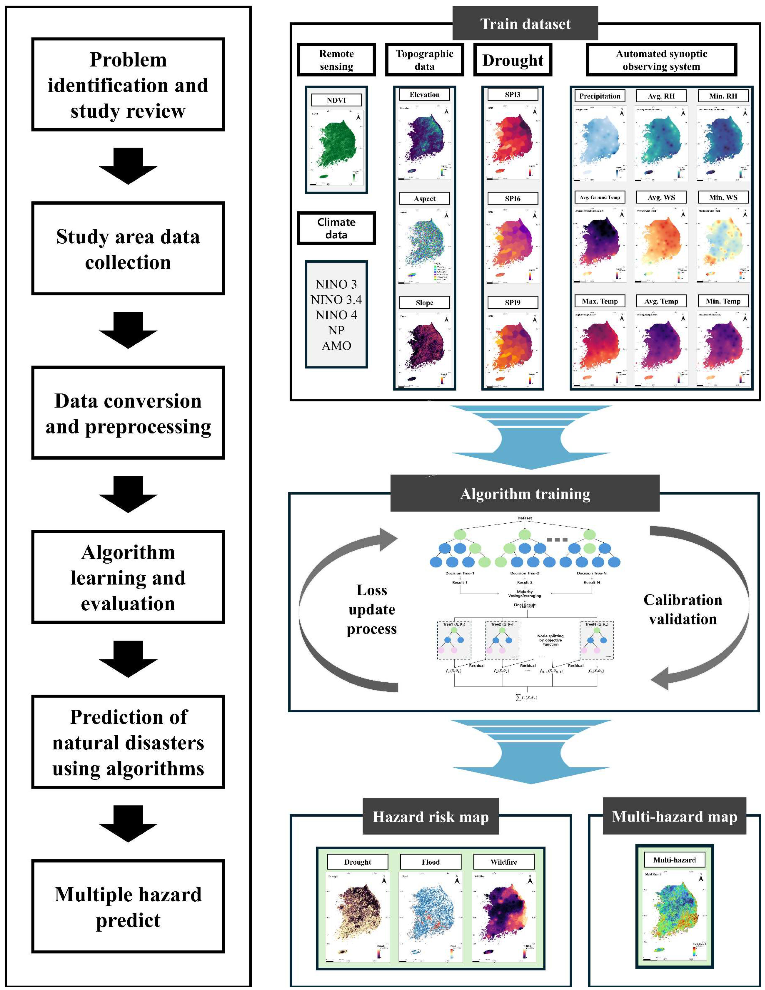
2. Materials and Methods

2.1. Study Area

The study area, as shown in Figure 1, encompasses the East Asian region between 38°36′49″N to 33°06′40″N and 124°36′35″E to 131°52′22″E. Covering approximately 100,210 km², the region lies within a mid-latitude temperate climate zone and experiences four distinct seasons. Over 50% of the annual precipitation is concentrated in July and August, with more than 700 mm of the average annual total of 1300 mm occurring during the summer monsoon. This seasonal concentration results in significant variability in rainfall runoff processes. Geographically, approximately 63% (62,980 km²) of the land is forested, with slopes exceeding 20%, resulting in rapid surface runoff during rainfall events. These characteristics present challenges for water resource management and increase the region’s vulnerability to hydrological hazards such as droughts and floods. Furthermore, the extensive forest cover combined with prolonged dry periods heightens the risk of hazards, such as wildfires.

2.2. Datasets

The datasets used in this study are listed in

Table 1. Input data for each natural hazard.

Category	Variable	Drought	Flood	Wildfire
Meteorological data	Precipitation (mm/day)	√	√	√
	Maximum temperature (°C)	√	√	√
	Minimum temperature (°C)	√	√	X
	Average temperature (°C)	√	√	X
	Average ground temperature (°C)	√	√	X
	Minimum relative humidity (%)	√	√	√
	Average relative humidity (%)	√	√	X
	Maximum wind speed (m/s)	√	√	√
	Average wind speed (m/s)	√	√	X
Drought data	SPI 3	X	√	√
	SPI 6	X	√	√
	SPI 9	X	√	√
Remote sensing data	NDVI	√	√	√
Date	Month	X	X	√
Topographic data	Digital elevation model	√	√	√
	Aspect	√	√	√
	Slope	√	√	√
Climate data	NINO 3	√	√	X
	NINO 3.4			X
	NINO 4			√
	North Pacific Index (NP)	√	√	√
	Atlantic Multidecadal Oscillation (AMO)	√	√	√

. The study area was transformed into a grid format with a resolution of 0.01°, and corresponding data for each grid cell were compiled and converted into a raster format for analysis. The grid-cell data were then preprocessed into a format suitable for algorithm training through the following steps:

First, geographic information—such as observation stations or natural hazard occurrence points—was converted into coordinates. The inverse distance-weighted (IDW) interpolation method was applied to generate raster data, ensuring spatial continuity during grid conversion. The power parameter of the IDW method was adjusted based on the characteristics of each dataset: a standard value of 2 was used for meteorological data due to the wide and sufficient distribution of observation stations, whereas a higher value of 3 was applied to drought indices to account for the increased interpolation uncertainty resulting from the sparse distribution of monitoring points.

Second, the study area was divided into 0.01° grid cells, and corresponding values were assigned to each grid point to create a reference grid. This reference grid served as a unified spatial framework for aligning all training data.

Third, after aligning the training data with the reference grid, the data were reorganized into a time-series table format suitable for input into machine learning algorithms. These preprocessing steps ensured that all data used in the study were standardized for model training.

2.2.1. Meteorological and Drought Data

Meteorological observation and climate data provided by South Korea’s Public Data Portal (https://www.data.go.kr, accessed on 7 March 2025) were used to construct the dataset. The meteorological dataset consists of daily weather data collected over a 24-year period (2000–2023). As of 2023, 105 synoptic weather observation stations have been installed nationwide. Data from 75 stations with sufficient observations during the study period were selected for analysis.

The drought dataset was built using the SPI3, SPI6, and SPI9 indices. Drought-related data were obtained from 60 weather observation stations that have provided daily SPI data since 2000. Additionally, data from six stations that began reporting SPI data in 2018 were incorporated into the dataset.

2.2.2. Water-Level Data

Water-level data were obtained from South Korea’s National Water Resources Management Information System (https://www.wamis.go.kr, accessed on 18 February 2025). The dataset includes daily water-level observations from 2000 to 2023. Of the 631 nationwide water-level observation stations reviewed, data from 294 stations that reported warning-level thresholds were selected for analysis.

2.2.3. Wildfire Data

Wildfire data were sourced from the Korea Forest Service through the Public Data Portal (https://www.data.go.kr, accessed on 7 March 2025) and the annually published Wildfire Statistics Yearbook [24]. The dataset includes records of 416 wildfire events that occurred between 2000 and 2023, each with a damage area of at least 0.05 km². Each record includes information such as the date and time of occurrence, location, and area affected. The data were organized in tabular format, and location information was converted into geographic coordinates for analysis.

2.2.4. Topographic Data

Topographic data were obtained from the National Geographic Information Institute of South Korea (https://www.ngii.go.kr, accessed on 10 March 2025). The dataset includes a Digital Elevation Model (DEM), slope, and aspect, all derived from 30 m resolution data. For this study, the data were resampled to a 0.01° resolution and aligned with the reference grid of the study area.

2.2.5. Climate Indices Data

Monthly atmospheric and oceanic climate indices were collected from the National Oceanic and Atmospheric Administration (NOAA; https://www.psl.noaa.gov, accessed on 11 March 2025). The dataset spans 24 years (2000–2023) and was incorporated into the model.

2.2.6. Remote Sensing Data

Remote sensing data were sourced from the Moderate Resolution Imaging Spectroradiometer (MODIS), accessed via Google Earth Engine (https://earthengine.google.com, accessed on 12 October 2024). MODIS provides Normalized Difference Vegetation Index (NDVI) data for all of South Korea at spatial resolutions of 250 m, 500 m, and 1 km, updated every 16 days. This study used NVDI data at 1 km resolution.

2.3. Model Developments

In this study, binary encoding was applied during data preprocessing to predict natural hazards, specifically droughts, floods, and wildfires [25]. Droughts were defined based on SPI6 values: cases with SPI6 ≤ −1.5 were encoded as 1 (drought), while cases with SPI6 > −1.5 were encoded as 0 (no drought). For model training, SPI3, SPI6, and SPI9 data were excluded as input features. Floods were identified using warning water levels at each observation station: values exceeding the warning level were encoded as 1 (flood), and those below were encoded as 0 (no flood). Wildfires were defined based on their occurrence: observed wildfires were encoded as 1, and non-occurrence as 0. The learning, testing, and analysis of the model performed in this study were performed in python 3.12.2 version.

For each hazard type, 70% of the dataset was used for model training, while the remaining 30% was reserved for validation. The overall research workflow is illustrated in Figure 2.

2.4. Machine Learning Algorithms

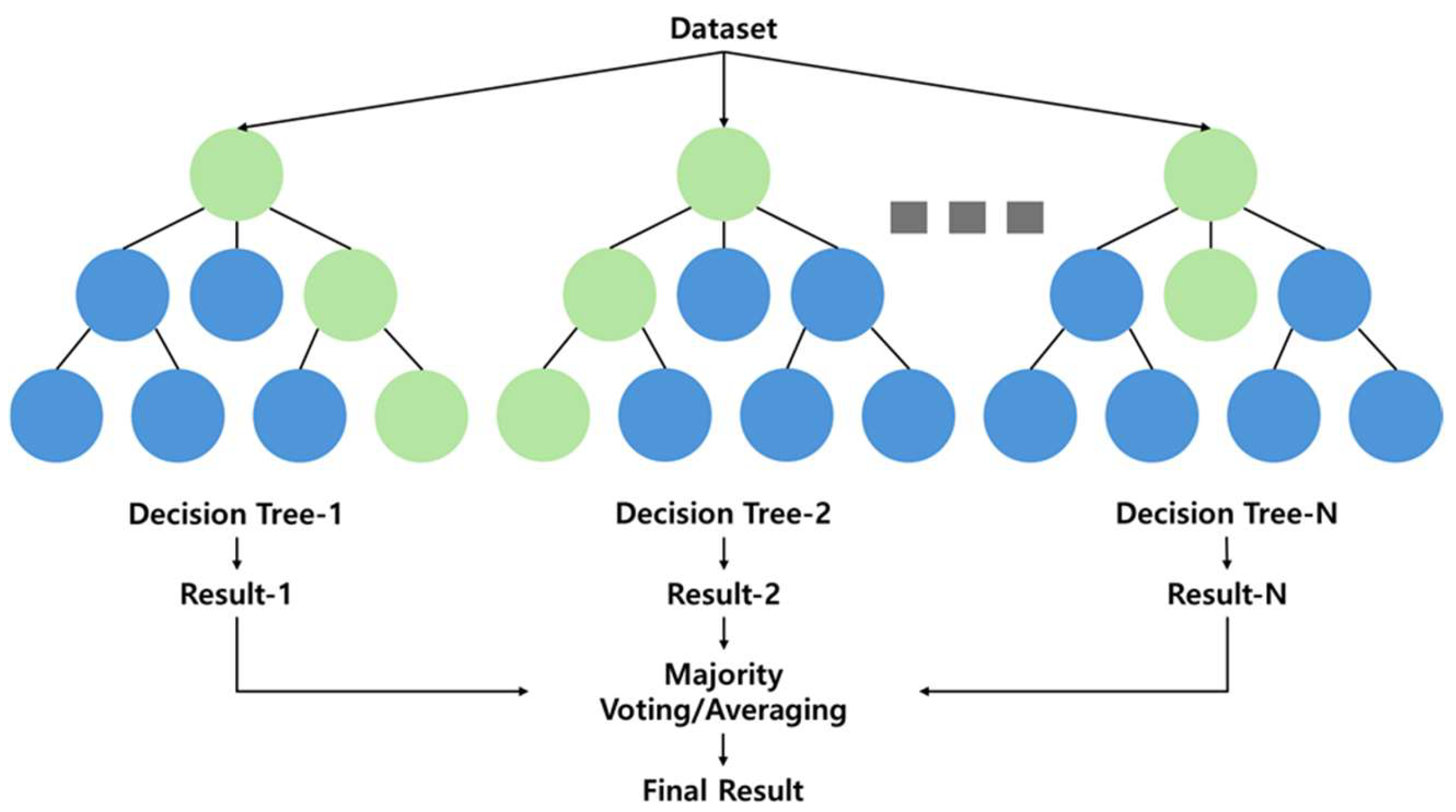
2.4.1. Random Forest

RF, proposed by Breiman (2001), is an ensemble learning model that improves predictive performance by combining multiple decision trees. It is a representative method of bagging (Bootstrap Aggregation) [26]. Bagging is a technique that creates subsets of the original dataset through bootstrapped sampling, which involves sampling with replacement. This process helps reduce the risk of overfitting in individual decision trees and enhances the overall generalization performance of the model. Figure 3 illustrates a schematic diagram of the Random Forest model. Each individual tree is trained on a subset of the training data generated through bagging, and during the node-splitting process, only a randomly selected subset of the total features is considered. This approach reduces the correlation among the trees and increases model diversity.

RF demonstrates strong performance against overfitting and maintains stable accuracy even with high-dimensional data. Furthermore, it reduces variance and enhances generalization performance by aggregating the predictions of individual trees through majority voting (for classification) or averaging (for regression) [27].

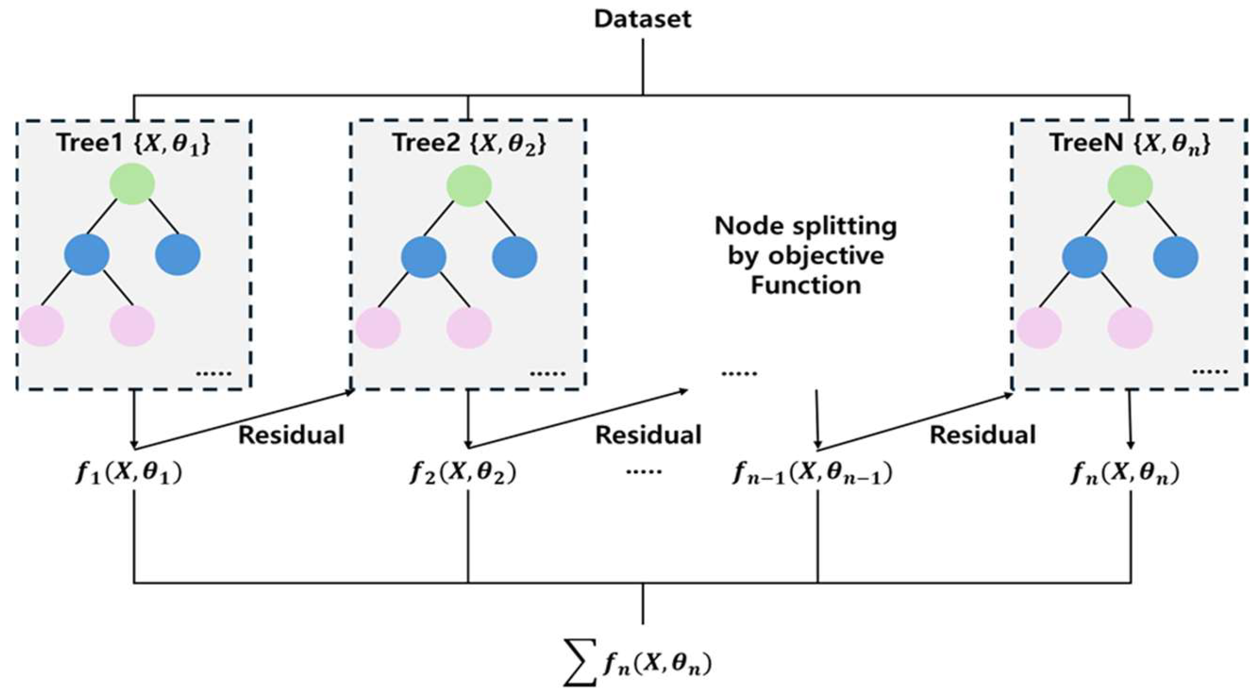
2.4.2. Extreme Gradient Boosting Architecture

XGB is a representative ensemble learning technique based on decision trees and is a type of boosting method. Boosting is an ensemble learning approach that combines multiple weak learners to build a highly accurate and robust classifier [28]. In this context, a weak learner typically refers to a shallow decision tree. During the sequential training process, these trees are trained in a way that assigns higher weights to the samples misclassified by the previous models, thereby gradually reducing the overall prediction error. A schematic of the XGB algorithm is shown in Figure 4.

XGB offers several advantages over other classification algorithms, including faster training speed, superior predictive performance, and the ability to handle missing values internally. Its tree-based structure also enables it to effectively solve nonlinear problems [29].

2.5. Evaluation Metrics

Classification evaluation metrics play a crucial role in achieving optimal classification during model training. While accuracy is often used for evaluating prediction and classification tasks, it has limitations—such as low discriminative power, limited decision-making capability, and bias toward the majority class. To address these issues, four performance metrics (

Table 2. Classification metrics.

		Observed
		Positive	Negative
Predictions	Positive	TP	FN
	Negative	FP	TN

) were used to evaluate model outcomes [30].

2.5.1. Accuracy

$$Accuracy={\displaystyle \frac{TP+TN}{TP+TN+FP+FN}}$$

(1)

Accuracy is a performance metric that represents how accurately the model predicts during the entire learning process. As shown in Equation (1), it is calculated by dividing the sum of true positives (TPs) and true negatives (TNs) by the total number of instances. While useful for balanced datasets, accuracy can be misleading in cases of class imbalance. The value ranges from 0 to 1, with values closer to 1 indicating higher predictive accuracy.

2.5.2. Precision

$$Precision={\displaystyle \frac{TP}{TP+FP}}$$

(2)

Precision is a performance metric that represents the proportion of true positive predictions among all instances predicted as positive. As shown in Equation (2), it is calculated by dividing TP by the sum of TP and false positives (FPs). This metric focuses on minimizing FP in order to maximize TP. Precision ranges from 0 to 1, with values closer to 1 indicating higher predictive accuracy.

2.5.3. Recall

$$Recall={\displaystyle \frac{TP}{TP+FN}}$$

(3)

Recall represents the proportion of actual positive cases correctly identified by the model. As shown in Equation (3), it is calculated by dividing TP by the sum of TP and false negatives (FNs). Recall is critical when missing positive cases could lead to significant consequences, as it focuses on minimizing FN to improve prediction accuracy. Recall ranges from 0 to 1, with values closer to 1 indicating higher predictive performance.

2.5.4. F1-Score

$$F1-score=2·{\displaystyle \frac{Precision·Recall}{Precision+Recall}}$$

(4)

F1-score is the harmonic mean of precision and recall, providing a balanced evaluation when both measures are required. When training with multivariate data that exhibit class imbalance, the F1-score offers a more comprehensive assessment than accuracy alone. It ranges from 0 to 1, with values closer to 1 indicating higher predictive accuracy (Equation (4)).

3. Results

3.1. Optimization Results

In this study, the natural hazard datasets were generally imbalanced, as occurrences of specific natural hazards were relatively rare compared to non-occurrence cases.

Table 3. Class distribution and occurrence rates for drought, flood, and wildfire datasets.

Parameters	Drought	Flood	Wildfire
Total Cases	2,489,260	6,891,358	3,646,240
Occurrence Cases	168,173	2189	416
Occurrence Rate	6.75%	0.03%	0.01%

illustrates the degree of data imbalance for each hazard. This imbalance increases the likelihood of performance degradation during model training. To mitigate the effects of data imbalance, algorithm-specific weight parameters were applied.

Weight calculations for each algorithm were either optimized using GridSearchCV or derived through algorithm-specific formulae. For the RF algorithm, weights were computed using Equation (5), while for XGB, weights were calculated using Equation (6):

$${Weight}_{RF}={\displaystyle \frac{TO}{NOC\times OIC}}$$

(5)

$${Weight}_{XGB}={\displaystyle \frac{OIC}{NOC}}$$

(6)

where TO the total number of observations, NOC is the number of classes, and OIC is the number of observations in a given class.

To further enhance performance, hyperparameters were optimized using GridSearchCV. For RF, both the Gini impurity and entropy were considered as classification criteria. The Gini impurity yielded superior results across drought and flood. Gini impurity is defined by Equation (7). However, in the case of wildfire prediction, entropy outperformed the Gini index, as defined in Equation (8).

$$\mathrm{Gini}\mathrm{impurity}=1-{\sum }_{i=1}^c{\left(P_i\right)}^2$$

(7)

$$\mathrm{entropy}=-{\sum }_{i=1}^C{P}_i{\log }_2\left(P_i\right)$$

(8)

where C represents the number of classes, and P_i denotes the proportion of class i within the given population.

The optimal hyperparameter combinations for each natural hazard type, derived using GridSearchCV, are summarized in

Table 4. Algorithm-specific parameter adjustment results.

Model	Parameters	Drought	Flood	Wildfire
RF	class_weight	Balanced	Balanced	Balanced
	Criterion	Gini	Gini	Gini
	max_depth	100	150	8
	max_features	-	-	2
	min_samples_leaf	8	8	1
	min_samples_split	8	2	4
	n_estimators	100	300	150
XGB	scale_pos_weight	Class Imbalance Ratio	Class Imbalance Ratio	2.583
	max_depth	9	9	4
	learning_rate	0.3	0.3	0.01
	subsample	0.9	0.9	0.6
	colsample_bytree	0.7	0.7	0.7

. To address class imbalance across all hazard datasets, the class_weight parameter in the Random Forest model was set to “balanced”. Additionally, for the wildfire dataset, random under-sampling was applied.

In the XGB algorithm, data imbalance was addressed using the scale_pos_weight parameter. Specifically for wildfires, downsampling was first applied, and an optimal weight of 2.583 was selected using GridSearchCV. The model parameters were then adjusted accordingly for training.

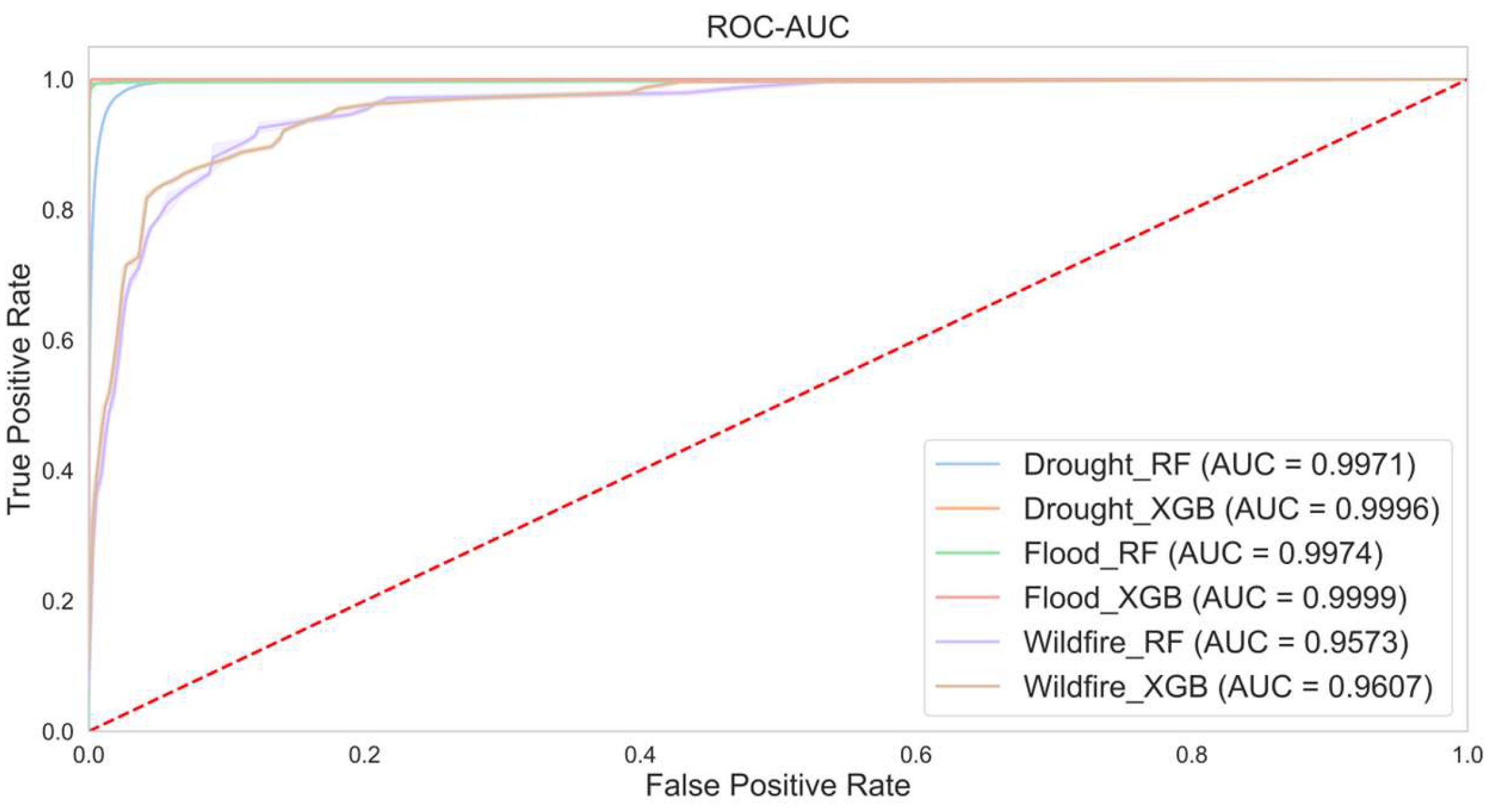
3.2. Modeling Performance

In this study, the predictive performances of the RF and XGB algorithms were compared across three types of natural hazards: drought, flood, and wildfire. Additionally, a feature importance analysis using the RF and XGB algorithms was conducted to identify key predictive variables for each hazard type. Model performance was evaluated using accuracy, precision, recall, and F1-score, with results summarized in

Table 5. Algorithm performance based on different metrics.

	Accuracy	Precision	Recall	F1-Score
Drought_RF	0.9817	0.8014	0.9669	0.8764
Drought_XGB	0.9974	0.9744	0.9873	0.9808
Flood_RF	0.9998	0.7437	0.6319	0.6833
Flood_XGB	0.9999	0.9198	0.9141	0.9169
Wildfire_RF	0.9073	0.7842	0.9008	0.8385
Wildfire_XGB	0.8940	0.7626	0.8760	0.8154

.

For drought prediction, XGB demonstrated superior performance across all evaluation metrics, achieving an accuracy of 0.9974, precision of 0.9744, recall of 0.9873, and an F1-score of 0.9808. In contrast, the RF algorithm yielded an accuracy of 0.9817, precision of 0.8014, recall of 0.9669, and F1-score of 0.9808, indicating overall lower predictive performance (Table 5).

In flood prediction, XGB again outperformed RF on all evaluation metrics. XGB achieved an accuracy of 0.9999, precision of 0.9198, recall of 0.9141, and an F1-score of 0.9169, demonstrating superior predictive performance. Although RF also showed a high accuracy of 0.9998, its precision (0.7437) and recall (0.6319) were considerably lower, resulting in an F1-score of 0.6833. These results indicate that RF had reduced effectiveness in identifying minority class instances in binary classification tasks (Table 5).

For wildfire prediction, RF outperformed XGB across all evaluation metrics. RF achieved an accuracy of 0.9073, precision of 0.7842, recall of 0.9008, and an F1-score of 0.8385, whereas XGB recorded an accuracy of 0.8940, precision of 0.7626, recall of 0.8760, and an F1-score of 0.8154. These results demonstrate that RF provided consistently superior predictive performance compared to XGB (Table 5).

Figure 5 presents a comparison of ROC-AUC performance between RF and XGB across the three hazard types. Both models demonstrated high ROC-AUC values, indicating excellent classification capabilities. For drought prediction, XGB achieved an AUC of 0.9998, outperforming RF (0.9971). For flood prediction, XGB exhibited near-perfect classification, while RF closely followed with an AUC of 0.9974. In wildfire prediction, XGB slightly outperformed RF, achieving an AUC of 0.9607 compared to 0.9573 for RF.

3.3. Feature Importance Analysis

To predict susceptibility levels for each natural hazard, model training was conducted, followed by a feature importance analysis using RF and XGB algorithms. The results are presented in Figure 6, which illustrates the ranking of variables based on their contribution to the occurrence of each hazard. In the case of RF, feature importance was calculated based on impurity decrease, and the contribution of each variable was normalized to a value between zero and one. For XGB, importance was assessed by the average reduction in loss during gradient updates, indicating how much each feature contributed to minimizing prediction error over the course of boosting iterations. This analysis identified the most influential features in the dataset, ranked according to their impact on prediction outcomes.

Figure 6a,b present the feature importance analysis results for the drought susceptibility model. Among the 16 input variables, the most influential factors in both models were NINO 3.4 and NINO 3, both classified as climatic factors. In addition to climate variables, the Digital Elevation Model (DEM) also exhibited significant influence. These results indicate that the El Niño-Southern Oscillation (ENSO) index plays a crucial role in drought occurrence [31]. Droughts appear to be more strongly affected by long-term climatic variations than by short-term meteorological changes. The relatively low importance of precipitation in drought prediction may be attributed to the use of daily precipitation data, which do not adequately capture the cumulative deficits responsible for droughts.

Figure 6c,d present the feature importance analysis for the flood susceptibility model. Among the 19 variables, precipitation was identified as the most influential factor, confirming its direct impact on flood occurrence. The second most important variable varied between the two models; however, both consistently emphasized the importance of climatic indicators. In the RF model, minimum relative humidity exhibited a high level of importance, which is likely to reflect the tendency for humidity to increase during rainfall events. In South Korea, floods are primarily triggered by intense monsoon-induced rainfall [32], underscoring the relevance of meteorological variables such as precipitation and humidity, as well as periodic climate indices in flood prediction.

Figure 6e,f present the feature importance analysis results for the wildfire susceptibility model. The most influential factors were minimum relative humidity, followed by the month of observation, and maximum wind speed. These findings indicate that wildfires are more likely to occur under dry conditions, with high temperatures increasing wind speed playing a critical role in fire spread.

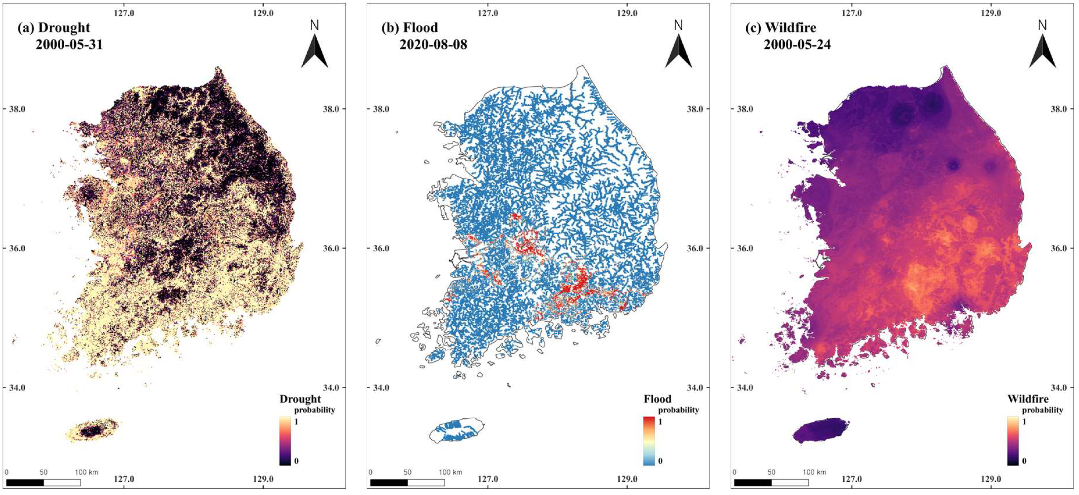
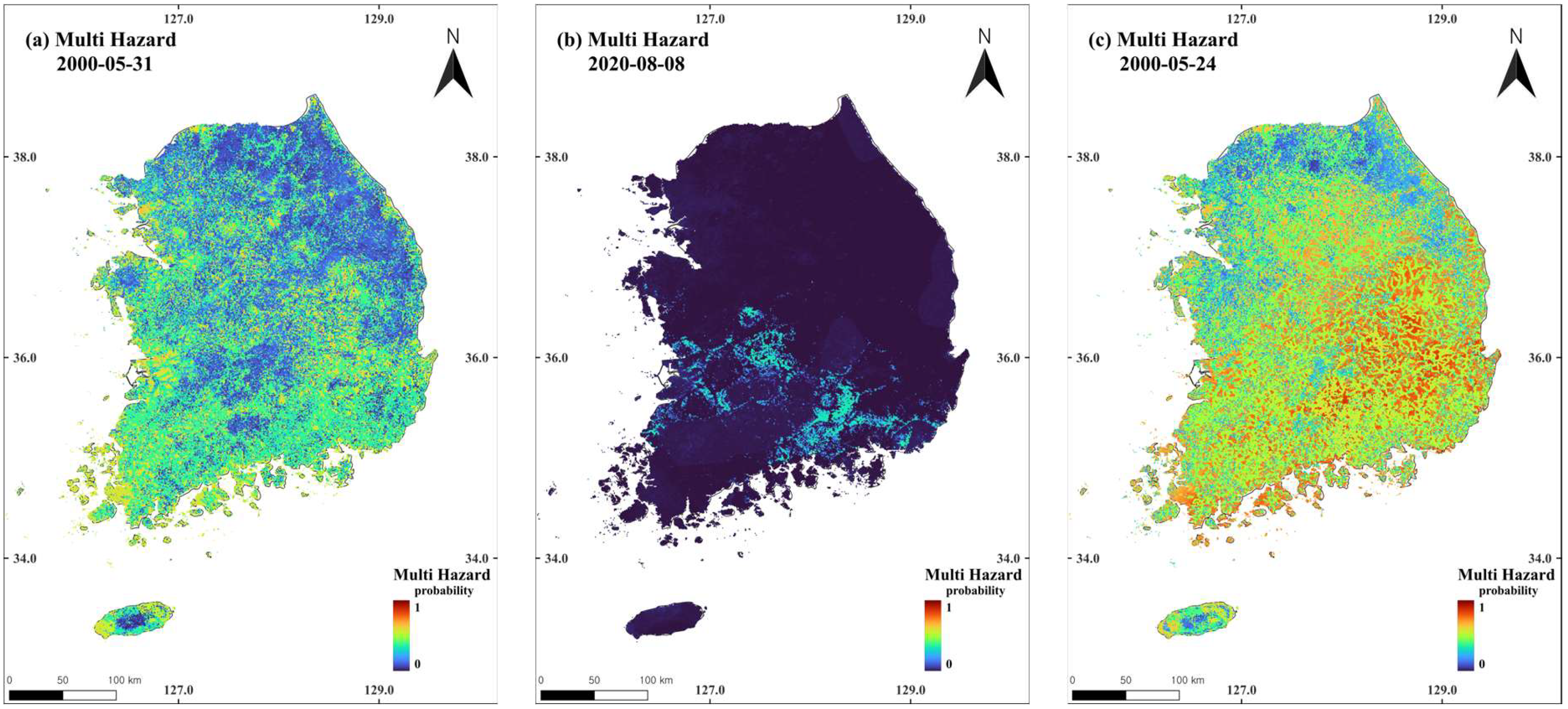
3.4. Multi-Hazard Prediction and Mapping of Susceptibility in South Korea

Figure 7 presents a visualization of the predicted probabilities of natural hazards (droughts, floods, wildfires, and multi-hazards) for the years 2000 and 2020, based on the results of the prediction models. Figure 7a,b show the drought susceptibility predictions, with high susceptibility in the 2000s corresponding to a period of low precipitation. In contrast, 2020, which experiences higher precipitation, showed lower drought susceptibility. Figure 7c,d show the flood susceptibility results. While most areas were predicted to have low flood susceptibility, certain regions showed high susceptibility in August 2020. Figure 7e,f present wildfire susceptibility, illustrating that wildfire-prone areas varied on a daily basis rather than remaining spatially consistent. Finally, Figure 7g,h show the predicted susceptibility to multi-hazards, visualizing overlapping risks from droughts, floods, and wildfires.

According to the Wildfire Statistics Yearbook [33], multiple large wildfires occurred in 2000 in the East Coast region, including Samcheok, Gangneung, and Donghae. The predicted wildfire susceptibility in Figure 7e aligns with these records, demonstrating the model’s effectiveness. Similarly, the National Drought Information Statistics Report [34] notes that beginning in April 2000, water shortages and restrictions were implemented in southern areas (Yeongnam and Honam). The model’s drought susceptibility predictions for this period, shown in Figure 8a, also reflect actual drought conditions. Furthermore, the Hazard Yearbook [35] reports severe flooding due to heavy rainfall in August 2020 in the central region. This event is reflected in the flood susceptibility map shown in Figure 7d, while Figure 8b highlights areas of high flood susceptibility during the same period.

Figure 8 presents susceptibility maps generated using the prediction models for drought, flood, and wildfire hazards. Each map represents predicted probabilities ranging from zero to one, with higher values indicating higher likelihoods of hazard occurrence. The drought and wildfire susceptibility maps (Figure 8a,c) were generated across the entire study area using 0.01° resolution grid data (125,028 pixels). The flood susceptibility map (Figure 8b) covers 65,889 pixels along river boundaries and includes a 0.01° buffer zone.

Hazard susceptibility levels were classified into five categories: Very Low (0–0.2), Low (0.2–0.4), Moderate (0.4–0.6), High (0.6–0.8), and Very High (0.8–1).

Table 6. Table of susceptibility ratings for each hazard visualized in Figure 8a–c.

	Drought (%)	Flood (%)	Wildfire (%)
Very Low (0–0.2)	32.01 (40,030)	90.76 (59,802)	49.18 (61,488)
Low (0.2–0.4)	6.46 (8075)	2.23 (1469)	23.41 (29,264)
Moderate (0.4–0.6)	5.66 (7073)	1.80 (1189)	8.89 (11,118)
High (0.6–0.8)	7.31 (9141)	5.20 (3429)	9.15 (11,441)
Very High (0.8–1)	48.56 (60,709)	0 (0)	9.31 (11,717)

presents the proportions of land area corresponding to each susceptibility category for each hazard type.

Figure 9 presents a multi-hazard susceptibility map that integrates the prediction results of the drought, flood, and wildfire models. Each hazard was modeled using the optimal algorithm (XGB for drought and flood, RF for wildfire), and the results were combined to assess overall hazard susceptibility. Figure 9a,c indicate that coastal areas along the East Sea exhibit a high likelihood of simultaneous natural hazard occurrences. Figure 9c, corresponding to an early severe drought period, shows high susceptibility levels, whereas Figure 9a, which represents a period of lower drought susceptibility, indicates a generally reduced multi-hazard threat. This demonstrates the model’s capability to reflect environmental changes influencing multi-hazard susceptibility. Figure 9b, representing the heavy rainfall period in 2020, shows near-zero susceptibility to drought and wildfire, but highlights high flood susceptibility in river basins across the central and southern regions that experienced severe flood damage.

4. Discussion

In recent decades, the frequency and magnitude of natural hazards have increased due to climate change and extreme weather events [36]. These hazards can occur independently but also tend to emerge simultaneously or interact with one another, amplifying their overall impact [37]. For example, prolonged drought reduces soil moisture and increases the likelihood of wildfires, which in turn consume vegetation on slopes and lead to increased direct runoff [38,39]. Previous studies have primarily focused on developing prediction models or analyzing factors influencing individual hazard types, such as droughts, floods, and wildfires [40,41,42].

This study trained prediction models for three types of natural hazards—droughts, floods, and wildfires—using two machine learning algorithms: RF and XGB. Based on these models, a multi-hazard susceptibility map was generated. The study quantitatively analyzed the spatial distribution of natural hazards and visualized areas with a high probability of hazard occurrence.

The key findings of this study are as follows: Optimal algorithms were selected for each hazard type, and prediction models were developed accordingly. XGB outperformed RF in predicting drought and flood events. These findings align with those of Sanders et al. [43], who demonstrated the superior performance of XGB in flood prediction, and Zhang et al. [44] in drought prediction. The results suggest that XGB is well-suited for capturing the nonlinear characteristics inherent in hazard data. In contrast, RF exhibited superior performance in wildfire prediction, consistent with previous studies highlighting its strong predictive capabilities for wildfires [45,46]. This suggests that RF effectively captures the interactions among wildfire-related variables, which is a key factor in wildfire prediction.

Feature importance analysis revealed that large-scale climate factors, such as ENSO indices (NINO 3.4, NINO 3, etc.), were key variables in drought prediction, highlighting the strong association between droughts and large-scale climate variability [47,48,49]. For flood prediction, precipitation and minimum relative humidity were identified as the most influential variables, indicating the direct influence of meteorological factors on flood events [50,51]. In wildfire prediction, minimum relative humidity and wind speed were found to be key variables, highlighting the critical role of dry conditions and strong winds in wildfire occurrence [52,53].

The multi-hazard susceptibility map identified the coastal areas along the East Sea as regions with high susceptibility to multi-hazards involving droughts, floods, and wildfires. These findings are consistent with those of Piao et al. [54], who predicted wildfire occurrences in this region. The identification of regions vulnerable to multiple hazards can serve as critical baseline data for hazard management and resource allocation strategies [55,56]. This study provides a framework for assessing the likelihood of concurrent natural hazards through multi-hazard susceptibility mapping.

Despite these contributions, the study has several limitations. First, the dataset used was limited to a specific temporal and spatial range, which may restrict the prediction accuracy in areas with low data density. Second, in wildfire prediction, certain variables, such as population density and anthropogenic factors, were not sufficiently incorporated, which could act as potential limitations affecting model performance. Third, the study did not quantitatively evaluate the interactions between multiple hazards. For example, the impact of drought on wildfire occurrence was not explicitly modeled, which should be addressed in future research.

Future research should expand the temporal and spatial scopes of the dataset to improve model accuracy. Additionally, it is necessary to model the simultaneity and interactions between multiple hazards to conduct an in-depth analysis of the mechanisms driving multi-hazard occurrences. Further efforts should focus on leveraging algorithms to learn complex relationships within the data and enhance the predictive performance.

In conclusion, this study successfully developed predictive models for droughts, floods, and wildfires and developed a multi-hazard susceptibility map, presenting new possibilities for hazard management. These findings demonstrate the effectiveness of machine learning and spatial data in hazard analysis and can serve as foundational data for future hazard management and resource allocation.

5. Conclusions

This study developed prediction models for three major natural hazards—droughts, floods, and wildfires—using machine learning algorithms (RF and XGB) and created a multi-hazard susceptibility map based on these models. The study results contribute to the quantitative assessment of hazard occurrence probabilities and the analysis of vulnerable areas prone to multi-hazards.

XGB demonstrated superior performance in drought and flood prediction, which can be attributed to its ability to effectively learn nonlinear data patterns. In wildfire prediction, RF outperformed XGB, likely due to its structural capability to capture the interactions between variables in wildfire data. Feature importance analysis revealed that, in drought prediction, large-scale climate factors such as ENSO indices (NINO 3.4, NINO 3, etc.) were the most influential variables, indicating a strong correlation between drought occurrence and large-scale climate patterns. For flood prediction, precipitation was identified as a key variable, while for wildfire prediction, minimum relative humidity, the month, and wind speed were the most significant factors. These findings contribute to a systematic understanding of the key factors influencing the occurrence of each hazard type.

Additionally, analysis of the multi-hazard susceptibility map identified the East Coast region as a vulnerable area with a high likelihood of experiencing multiple hazards, including droughts, floods, and wildfires. The development of a multi-hazard susceptibility map extends beyond a single-hazard analysis and serves as a foundational resource for understanding the complexity of multi-hazard management and formulating effective response strategies.

References

1. Wilhite, D.A.; Sivakumar, M.V.; Pulwarty, R. Managing drought risk in a changing climate: The role of national drought policy. Weather Clim. Extrem. 2014, 3, 4–13. [Google Scholar] [CrossRef]
2. Merz, B.; Kreibich, H.; Schwarze, R.; Thieken, A. Review article “Assessment of economic flood damage”. Nat. Hazards Earth Syst. Sci. 2010, 10, 1697–1724. [Google Scholar] [CrossRef]
3. Kappes, M.S.; Keiler, M.; von Elverfeldt, K.; Glade, T. Challenges of analyzing multi-hazard risk: A review. Nat. Hazards 2012, 64, 1925–1958. [Google Scholar] [CrossRef]
4. Wang, J.; He, Z.; Weng, W. A review of the research into the relations between hazards in multi-hazard risk analysis. Nat. Hazards 2020, 104, 2003–2026. [Google Scholar] [CrossRef]
5. Flannigan, M.D.; Stocks, B.J.; Wotton, B.M. Climate change and forest fires. Sci. Total Environ. 2000, 262, 221–229. [Google Scholar] [CrossRef]
6. Kelman, I.; Spence, R. An overview of flood actions on buildings. Eng. Geol. 2004, 73, 297–309. [Google Scholar] [CrossRef]
7. Plate, E.J. Flood risk and flood management. J. Hydrol. 2002, 267, 2–11. [Google Scholar] [CrossRef]
8. Wotton, B.M.; Nock, C.A.; Flannigan, M.D. Forest fire occurrence and climate change in Canada. Int. J. Wildland Fire 2010, 19, 253–271. [Google Scholar] [CrossRef]
9. Mishra, A.K.; Singh, V.P. A review of drought concepts. J. Hydrol. 2010, 391, 202–216. [Google Scholar] [CrossRef]
10. Svoboda, M.; LeComte, D.; Hayes, M.; Heim, R.; Gleason, K.; Angel, J.; Stephens, S. The drought monitor. Bull. Am. Meteorol. Soc. 2002, 83, 1181–1190. [Google Scholar] [CrossRef]
11. Luo, L.; Wood, E.F. Monitoring and predicting the 2007 US drought. Geophys. Res. Lett. 2007, 34, L22702. [Google Scholar] [CrossRef]
12. Moreira, E.E.; Coelho, C.A.; Paulo, A.A.; Pereira, L.S.; Mexia, J.T. SPI-based drought category prediction using loglinear models. J. Hydrol. 2008, 354, 116–130. [Google Scholar] [CrossRef]
13. Schumann, G.J.-P.; Neal, J.C.; Voisin, N.; Andreadis, K.M.; Pappenberger, F.; Phanthuwongpakdee, N.; Hall, A.C.; Bates, P.D. A first large-scale flood inundation forecasting model: Large-Scale Flood Inundation Forecasting. Water Resour. Res. 2013, 49, 6248–6257. [Google Scholar] [CrossRef]
14. Rocchi, A.; Chiozzi, A.; Nale, M.; Nikolic, Z.; Riguzzi, F.; Mantovan, L.; Benvenuti, E. A machine learning framework for multi-hazard risk assessment at the regional scale in earthquake and flood-prone areas. Appl. Sci. 2022, 12, 583. [Google Scholar] [CrossRef]
15. Khan, N.; Sachindra, D.A.; Shahid, S.; Ahmed, K.; Shiru, M.S.; Nawaz, N. Prediction of droughts over Pakistan using machine learning algorithms. Adv. Water Resour. 2020, 139, 103562. [Google Scholar] [CrossRef]
16. Pham, B.T.; Jaafari, A.; Avand, M.; Al-Ansari, N.; Dinh Du, T.; Yen, H.P.H.; Tuyen, T.T. Performance evaluation of machine learning methods for forest fire modeling and prediction. Symmetry 2020, 12, 1022. [Google Scholar] [CrossRef]
17. Fang, Z.; Wang, Y.; Peng, L.; Hong, H. Predicting flood susceptibility using LSTM neural networks. J. Hydrol. 2021, 594, 125734. [Google Scholar] [CrossRef]
18. Mohajane, M.; Costache, R.; Karimi, F.; Pham, Q.B.; Essahlaoui, A.; Nguyen, H.; Oudija, F. Application of remote sensing and machine learning algorithms for forest fire mapping in a Mediterranean area. Ecol. Indic. 2021, 129, 107869. [Google Scholar] [CrossRef]
19. Mosavi, A.; Ozturk, P.; Chau, K.W. Flood prediction using machine learning models: Literature review. Water 2018, 10, 1536. [Google Scholar] [CrossRef]
20. Sankaranarayanan, S.; Prabhakar, M.; Satish, S.; Jain, P.; Ramprasad, A.; Krishnan, A. Flood prediction based on weather parameters using deep learning. J. Water Clim. Change 2020, 11, 1766–1783. [Google Scholar] [CrossRef]
21. Antzoulatos, G.; Kouloglou, I.O.; Bakratsas, M.; Moumtzidou, A.; Gialampoukidis, I.; Karakostas, A.; Kompatsiaris, I. Flood hazard and risk mapping by applying an explainable machine learning framework using satellite imagery and GIS data. Sustainability 2022, 14, 3251. [Google Scholar] [CrossRef]
22. Iban, M.C.; Aksu, O. SHAP-driven explainable artificial intelligence framework for wildfire susceptibility mapping using MODIS active fire pixels: An in-depth interpretation of contributing factors in Izmir, Türkiye. Remote Sens. 2024, 16, 2842. [Google Scholar] [CrossRef]
23. Tilloy, A.; Malamud, B.D.; Winter, H.; Joly-Laugel, A. A review of quantification methodologies for multi-hazard inter-relationships. Earth Sci. Rev. 2019, 196, 102881. [Google Scholar] [CrossRef]
24. Korea Forest Service. 2022 Wildfire Statistics Yearbook; Korea Forest Service: Daejeon, Republic of Korea, 2023. [Google Scholar]
25. Syeed, M.M.A.; Farzana, M.; Namir, I.; Ishrar, I.; Nushra, M.H.; Rahman, T. Flood prediction using machine learning models. In Proceedings of the 2022 International Congress on Human-Computer Interaction, Optimization and Robotic Applications (HORA), Ankara, Turkey, 9–11 June 2022; pp. 1–6. [Google Scholar] [CrossRef]
26. Breiman, L. Random forests. Mach. Learn. 2001, 45, 5–32. [Google Scholar] [CrossRef]
27. Scornet, E.; Biau, G.; Vert, J.-P. Consistency of random forests. Ann. Statist. 2015, 43, 1716–1741. [Google Scholar] [CrossRef]
28. Chen, T.; Guestrin, C. XGBoost: A Scalable Tree Boosting System. In Proceedings of the 22nd ACM SIGKDD International Conference on Knowledge Discovery and Data Mining, San Francisco, CA, USA, 13–17 August 2016; ACM: New York, NY, USA, 2016; pp. 785–794. [Google Scholar] [CrossRef]
29. Ma, M.; Zhao, G.; He, B.; Li, Q.; Dong, H.; Wang, S.; Wang, Z. XGBoost-Based Method for Flash Flood Risk Assessment. J. Hydrol. 2021, 598, 126382. [Google Scholar] [CrossRef]
30. Hossin, M.; Sulaiman, M.N. A review on evaluation metrics for data classification evaluations. Int. J. Data Min. Knowl. Manag. Process 2015, 5, 1. [Google Scholar] [CrossRef]
31. En-Nagre, K.; Aqnouy, M.; Ouarka, A.; Naqvi, S.A.A.; Bouizrou, I.; El Messari, J.E.S.; El-Askary, H. Assessment and prediction of meteorological drought using machine learning algorithms and climate data. Clim. Risk Manage. 2024, 45, 100630. [Google Scholar] [CrossRef]
32. Ha, K.J.; Moon, S.; Timmermann, A.; Kim, D. Future changes of summer monsoon characteristics and evaporative demand over Asia in CMIP6 simulations. Geophys. Res. Lett. 2020, 47, e2020GL087492. [Google Scholar] [CrossRef]
33. Korea Forest Service. 2010 Wildfire Statistics Yearbook; Korea Forest Service: Daejeon, Republic of Korea, 2011. [Google Scholar]
34. Ministry of the Interior and Safety. 2018 National Drought Information Statistics Report; Ministry of the Interior and Safety: Sejong, Republic of Korea, 2020. [Google Scholar]
35. Korea Forest Service. 2020 Disaster Yearbook; Ministry of the Interior and Safety: Sejong, Republic of Korea, 2021. [Google Scholar]
36. Forzieri, G.; Feyen, L.; Russo, S.; Vousdoukas, M.; Alfieri, L.; Outten, S.; Cid, A. Multi-hazard assessment in Europe under climate change. Clim. Change 2016, 137, 105–119. [Google Scholar] [CrossRef]
37. Gill, J.C.; Malamud, B.D. Anthropogenic processes, natural hazards, and interactions in a multi-hazard framework. Earth Sci. Rev. 2017, 166, 246–269. [Google Scholar] [CrossRef]
38. Brogan, D.J.; Nelson, P.A.; MacDonald, L.H. Reconstructing extreme post-wildfire floods: A comparison of convective and mesoscale events. Earth Surf. Process. Landf. 2017, 42, 2505–2522. [Google Scholar] [CrossRef]
39. Richardson, D.; Black, A.S.; Irving, D.; Matear, R.J.; Monselesan, D.P.; Risbey, J.S.; Tozer, C.R. Global increase in wildfire potential from compound fire weather and drought. NPJ Clim. Atmos. Sci. 2022, 5, 23. [Google Scholar] [CrossRef]
40. Demissie, Z.; Rimal, P.; Seyoum, W.M.; Dutta, A.; Rimmington, G. Flood susceptibility mapping: Integrating machine learning and GIS for enhanced risk assessment. Appl. Comput. Geosci. 2024, 23, 100183. [Google Scholar] [CrossRef]
41. Hang, H.T.; Mallick, J.; Alqadhi, S.; Bindajam, A.A.; Abdo, H.G. Exploring forest fire susceptibility and management strategies in Western Himalaya: Integrating ensemble machine learning and explainable AI for accurate prediction and comprehensive analysis. Environ. Technol. Innov. 2024, 35, 103655. [Google Scholar] [CrossRef]
42. Zhang, B.; Salem, F.K.A.; Hayes, M.J.; Tadesse, T. Quantitative assessment of drought impacts using XGBoost based on the drought impact reporter. arXiv 2022, arXiv:2211.02768. [Google Scholar] [CrossRef]
43. Sanders, W.; Li, D.; Li, W.; Fang, Z.N. Data-driven flood alert system (FAS) using extreme gradient boosting (XGBoost) to forecast flood stages. Water 2022, 14, 747. [Google Scholar] [CrossRef]
44. Zhang, B.; Salem, F.K.A.; Hayes, M.J.; Smith, K.H.; Tadesse, T.; Wardlow, B.D. Explainable machine learning for the prediction and assessment of complex drought impacts. Sci. Total Environ. 2023, 898, 165509. [Google Scholar] [CrossRef]
45. Mehmood, K.; Anees, S.A.; Luo, M.; Akram, M.; Zubair, M.; Khan, K.A.; Khan, W.R. Assessing Chilgoza Pine (Pinus gerardiana) forest fire severity: Remote sensing analysis, correlations, and predictive modeling for enhanced management strategies. Trees For. People 2024, 16, 100521. [Google Scholar] [CrossRef]
46. Singha, C.; Swain, K.C.; Moghimi, A.; Foroughnia, F.; Swain, S.K. Integrating geospatial, remote sensing, and machine learning for climate-induced forest fire susceptibility mapping in Similipal Tiger Reserve, India. For. Ecol. Manage. 2024, 555, 121729. [Google Scholar] [CrossRef]
47. Abdelkader, M.; Yerdelen, C. Hydrological drought variability and its teleconnections with climate indices. J. Hydrol. 2022, 605, 127290. [Google Scholar] [CrossRef]
48. Abdourahamane, Z.S.; Acar, R. Analysis of meteorological drought variability in Niger and its connection with climate indices. Hydrol. Sci. J. 2018, 63, 1203–1218. [Google Scholar] [CrossRef]
49. Yue, Y.; Liu, H.; Mu, X.; Qin, M.; Wang, T.; Wang, Q.; Yan, Y. Spatial and temporal characteristics of drought and its correlation with climate indices in Northeast China. PLoS ONE 2021, 16, e0259774. [Google Scholar] [CrossRef]
50. Hakim, D.K.; Gernowo, R.; Nirwansyah, A.W. Flood prediction with time series data mining: Systematic review. Nat. Hazard. Res. 2024, 4, 194–220. [Google Scholar] [CrossRef]
51. Toth, E.; Brath, A.; Montanari, A. Comparison of short-term rainfall prediction models for real-time flood forecasting. J. Hydrol. 2000, 239, 132–147. [Google Scholar] [CrossRef]
52. Dong, H.; Wu, H.; Sun, P.; Ding, Y. Wildfire prediction model based on spatial and temporal characteristics: A case study of a wildfire in Portugal’s Montesinho Natural Park. Sustainability 2022, 14, 10107. [Google Scholar] [CrossRef]
53. Malik, A.; Rao, M.R.; Puppala, N.; Koouri, P.; Thota, V.A.K.; Liu, Q.; Gao, J. Data-driven wildfire risk prediction in northern California. Atmosphere 2021, 12, 109. [Google Scholar] [CrossRef]
54. Piao, Y.; Lee, D.; Park, S.; Kim, H.G.; Jin, Y.H. Multi-hazard mapping of droughts and forest fires using a multi-layer hazards approach with machine learning algorithms. Geomat. Nat. Hazards Risk 2022, 13, 2649–2673. [Google Scholar] [CrossRef]
55. Pourghasemi, H.R.; Kariminejad, N.; Amiri, M.; Edalat, M.; Zarafshar, M.; Blaschke, T.; Cerda, A. Assessing and mapping multi-hazard risk susceptibility using a machine learning technique. Sci. Rep. 2020, 10, 3203. [Google Scholar] [CrossRef]
56. Vitolo, C.; Di Napoli, C.; Di Giuseppe, F.; Cloke, H.L.; Pappenberger, F. Mapping combined wildfire and heat stress hazards to improve evidence-based decision making. Environ. Int. 2019, 127, 21–34. [Google Scholar] [CrossRef]
Figure 1. Study area relevant to the analysis: (a) the blue lines represent the river boundaries within the study region; (b) the blue triangles mark the locations of the weather stations; (c) the blue dots mark the locations of the water-level observatories; and (d) the red dots denote the locations of the wildfire damage sites.
Remotesensing 17 01660 g001
Figure 2. Flowchart of the study.
Remotesensing 17 01660 g002
Figure 3. Architecture of the Random Forest algorithm.
Remotesensing 17 01660 g003
Figure 4. Architecture of the Extreme Gradient Boosting algorithm.
Remotesensing 17 01660 g004
Figure 5. Performance comparison of algorithms by hazard type (ROC-AUC).
Remotesensing 17 01660 g005
Figure 6. Key variables affecting prediction: (a,b) drought, (c,d) flood, (e,f) wildfire. Left: RF; right: XGB.
Remotesensing 17 01660 g006
Figure 7. Temporal distribution of predictive probabilities for natural hazards: (a,b) floods in 2000 and 2020; (c,d) droughts in 2000 and 2020; (e,f) wildfires in 2000 and 2020; and (g,h) multi-hazards in 2000 and 2020. Each panel shows the temporal variation in grid occupancy (%) across probability ranges from zero to one on a daily resolution.
Remotesensing 17 01660 g007
Figure 8. Susceptibility map for natural hazards: (a) drought, (b) flood, and (c) wildfire.
Remotesensing 17 01660 g008
Figure 9. Susceptibility maps for multi-hazards (ac) show susceptibility distributions for three representative days selected from high-susceptibility periods.
Remotesensing 17 01660 g009