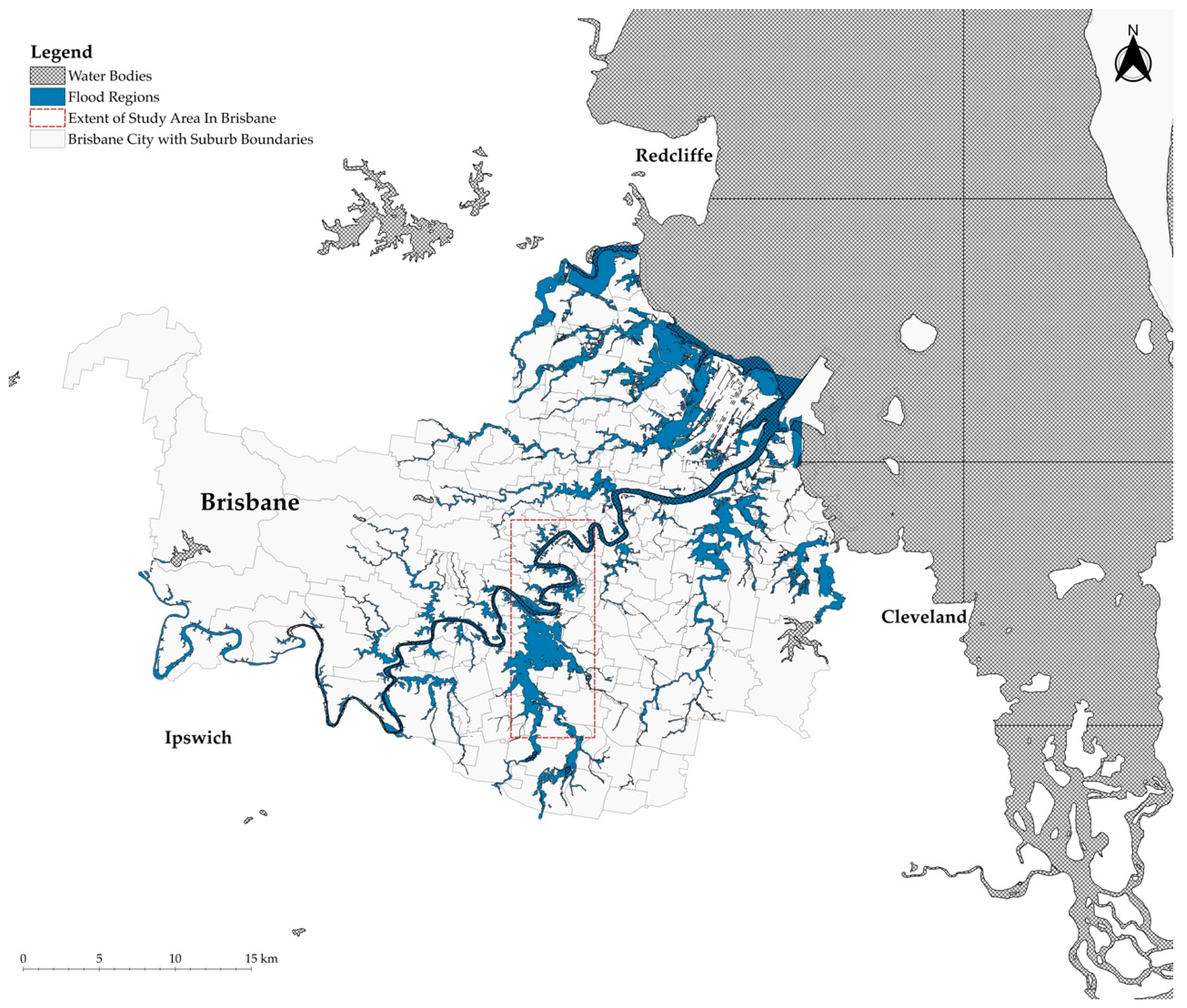
Figure 1.
The extent of flooding in Brisbane during February 2022. The figure, based on [
24], was created by combining Brisbane City Council (BCC) Flood Map [
47], and World Water Bodies shapefiles [
48].
Figure 1.
The extent of flooding in Brisbane during February 2022. The figure, based on [
24], was created by combining Brisbane City Council (BCC) Flood Map [
47], and World Water Bodies shapefiles [
48].
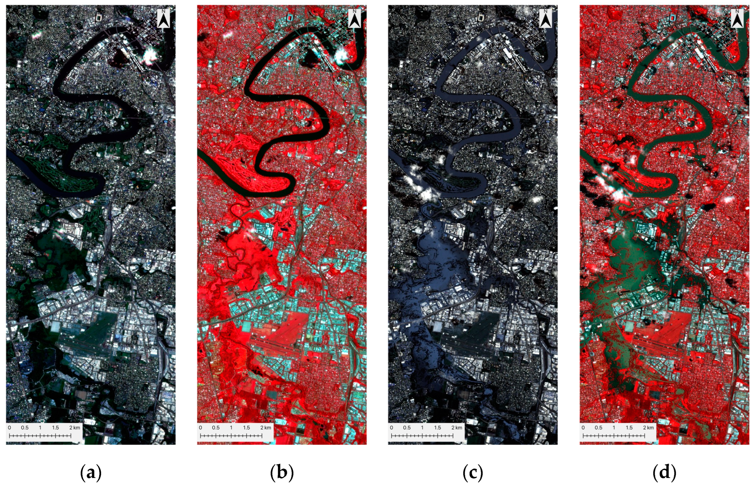
Figure 2.
Comparison of pre-flood (a) and peak-flood (c) images in true color and false color (NIR, R, G) composites (b,d). In the false color images (b,d), red indicates vegetation, dark olive green represents water bodies, and other colors depict buildings and urban areas.
Figure 2.
Comparison of pre-flood (a) and peak-flood (c) images in true color and false color (NIR, R, G) composites (b,d). In the false color images (b,d), red indicates vegetation, dark olive green represents water bodies, and other colors depict buildings and urban areas.
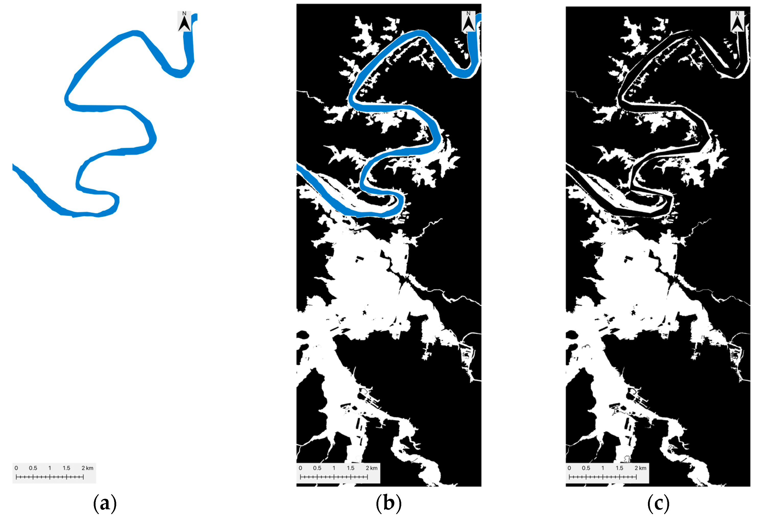
Figure 3.
Illustration of the creation of the labeled dataset image (c). It combines a river mask (a) with a flood extent map (b) to isolate flooded areas (white) while excluding the river (blue).
Figure 3.
Illustration of the creation of the labeled dataset image (c). It combines a river mask (a) with a flood extent map (b) to isolate flooded areas (white) while excluding the river (blue).
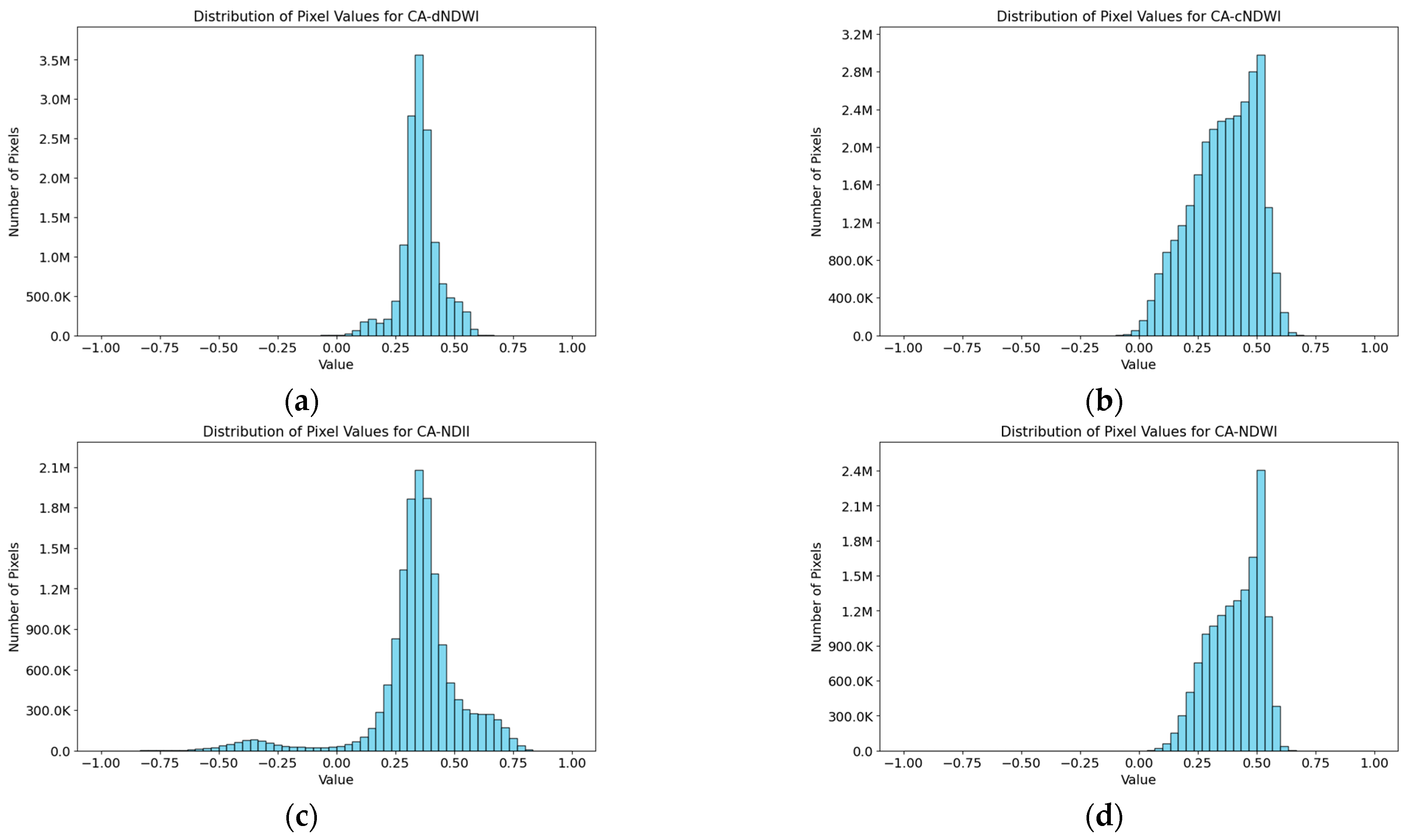
Figure 4.
Comparisons of the distribution of pixel values from all bands of each CA dataset, with (a–d) referring CA-dNDWI, CA-cNDWI, CA-NDII, and CA-NDWI.
Figure 4.
Comparisons of the distribution of pixel values from all bands of each CA dataset, with (a–d) referring CA-dNDWI, CA-cNDWI, CA-NDII, and CA-NDWI.
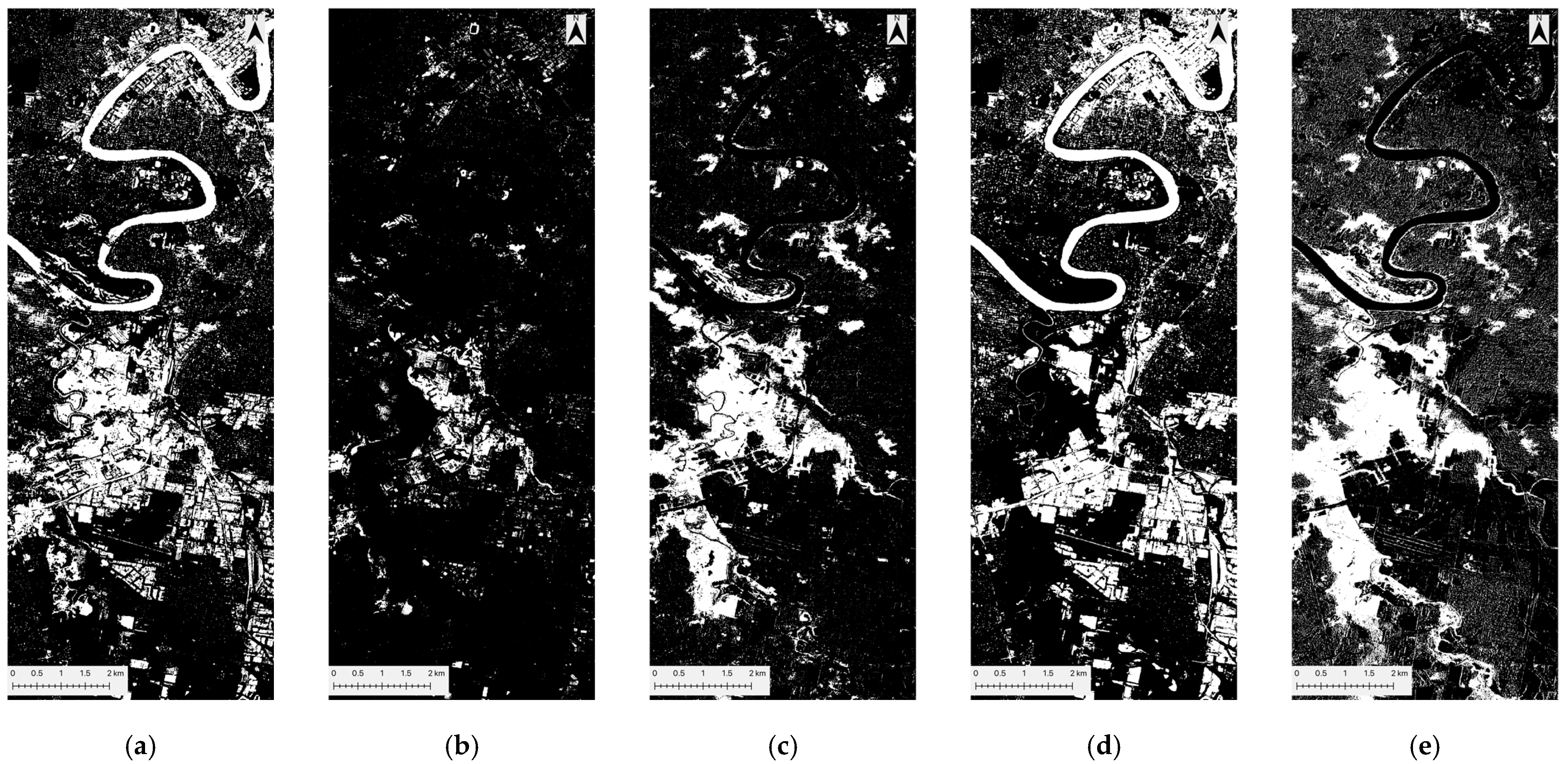
Figure 5.
Baseline flood maps. Each sub-figure delineates inundated water (white) from non-inundated areas (black), which include both permanent water and non-water areas. (a,b) depict the flood maps obtained by applying 0.2 and 0.3 thresholds to NDWIpeak-flood. (c) shows the flood map of NDII using a 0.1 threshold. (d) depicts the flood map of cNDWI using a 0.1 threshold. (e) delineates the flood map of dNDWI using a threshold of 0.2.
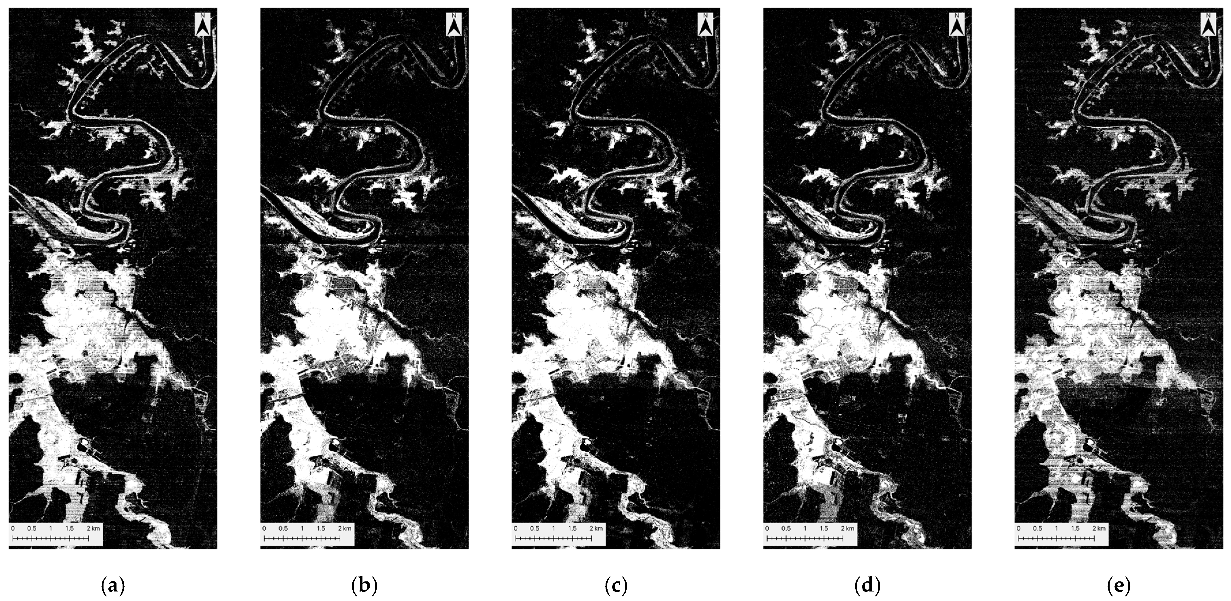
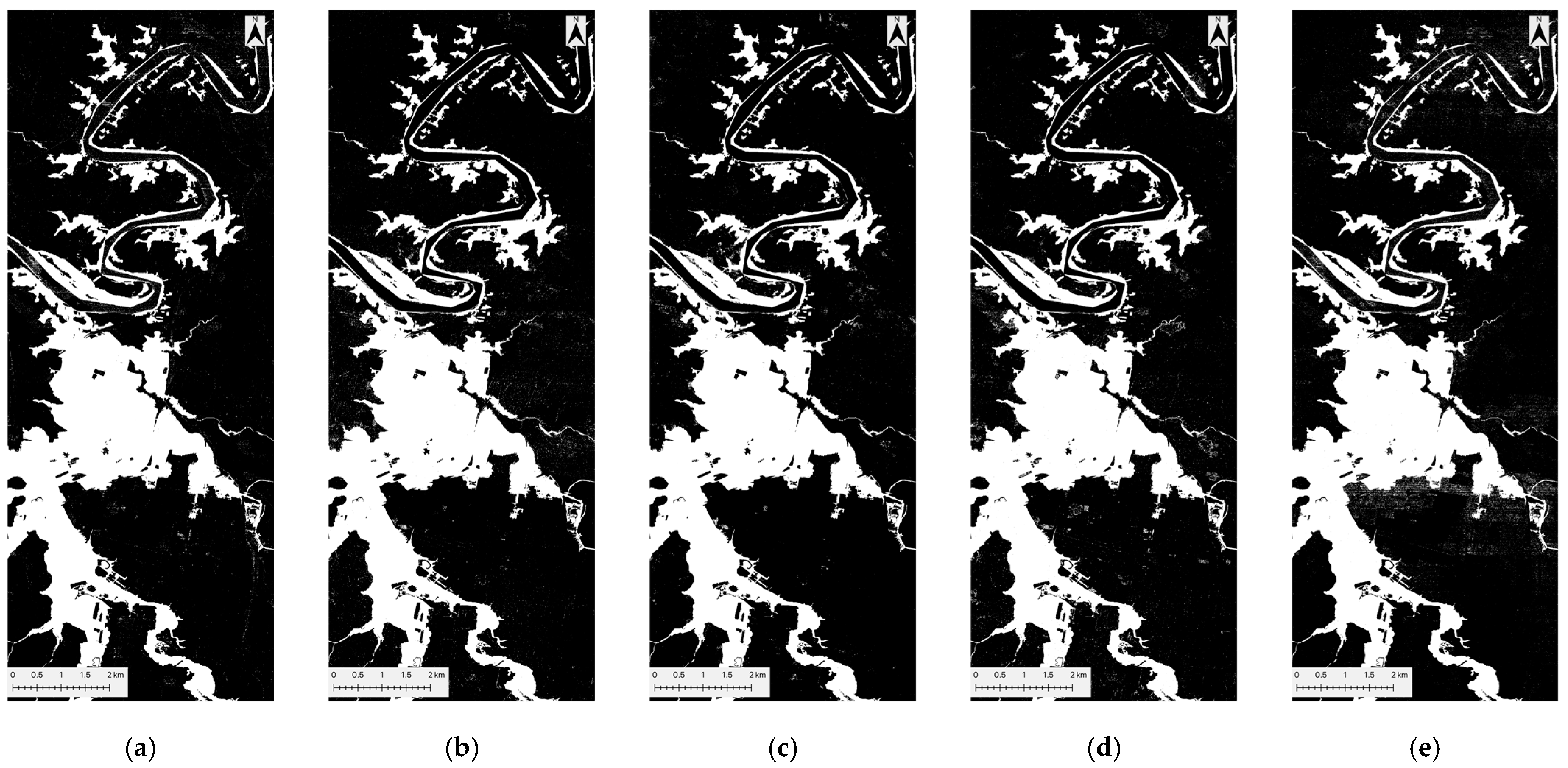
Figure 6.
KNN flood prediction maps for five datasets: (a) peak-flood image, (b) CA-dNDWI, (c) CA-cNDWI, (d) CA-NDII, and (e) CA-NDWI. Each sub-figure delineates inundated water (white) from non-inundated areas (black), which include both permanent water and non-water areas.
Figure 6.
KNN flood prediction maps for five datasets: (a) peak-flood image, (b) CA-dNDWI, (c) CA-cNDWI, (d) CA-NDII, and (e) CA-NDWI. Each sub-figure delineates inundated water (white) from non-inundated areas (black), which include both permanent water and non-water areas.
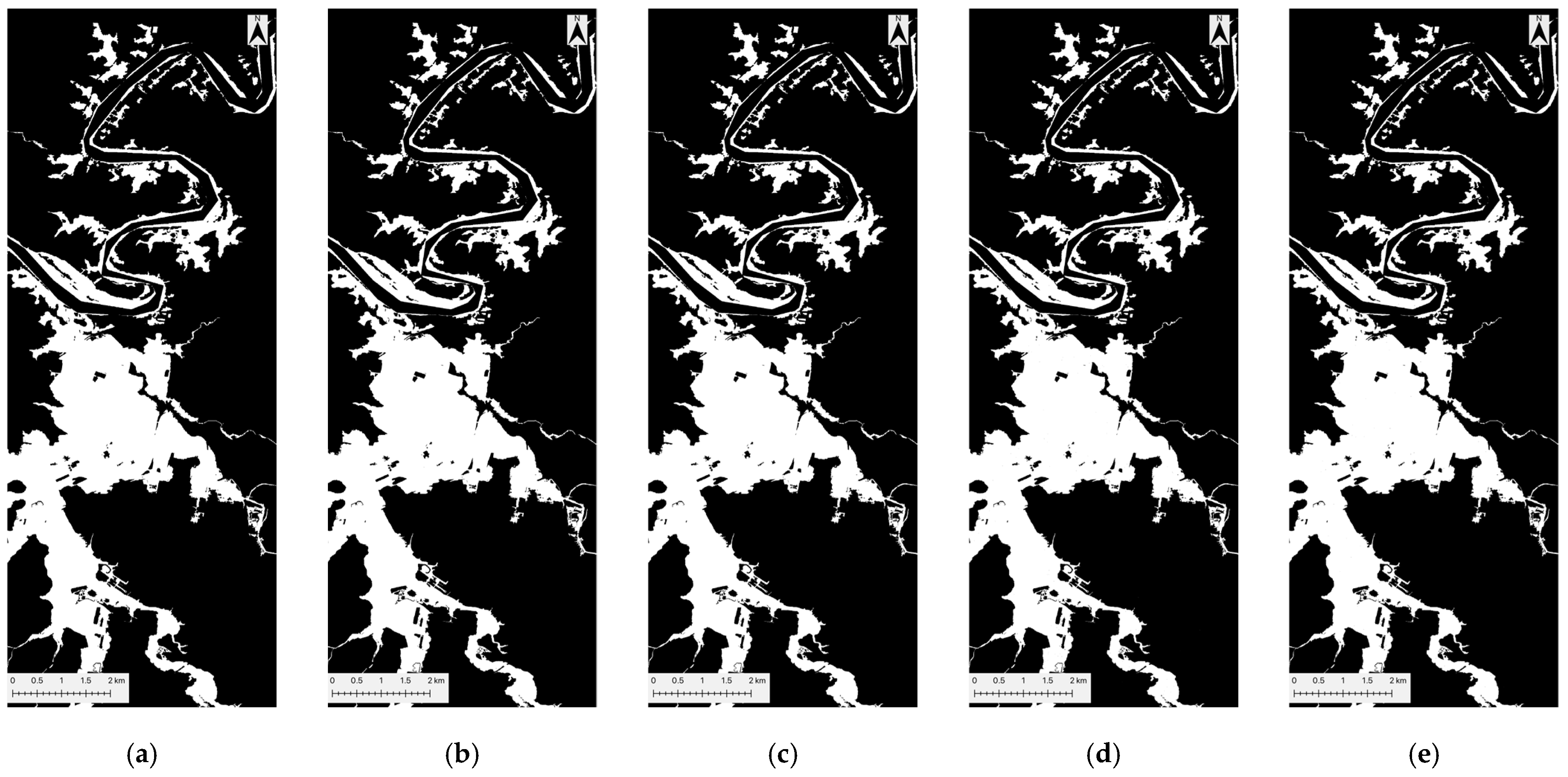
Figure 7.
GNB flood prediction maps for five datasets: (a) peak-flood image, (b) CA-dNDWI, (c) CA-cNDWI, (d) CA-NDII, and (e) CA-NDWI. Each sub-figure delineates inundated water (white) from non-inundated areas (black), which include both permanent water and non-water areas.
Figure 7.
GNB flood prediction maps for five datasets: (a) peak-flood image, (b) CA-dNDWI, (c) CA-cNDWI, (d) CA-NDII, and (e) CA-NDWI. Each sub-figure delineates inundated water (white) from non-inundated areas (black), which include both permanent water and non-water areas.
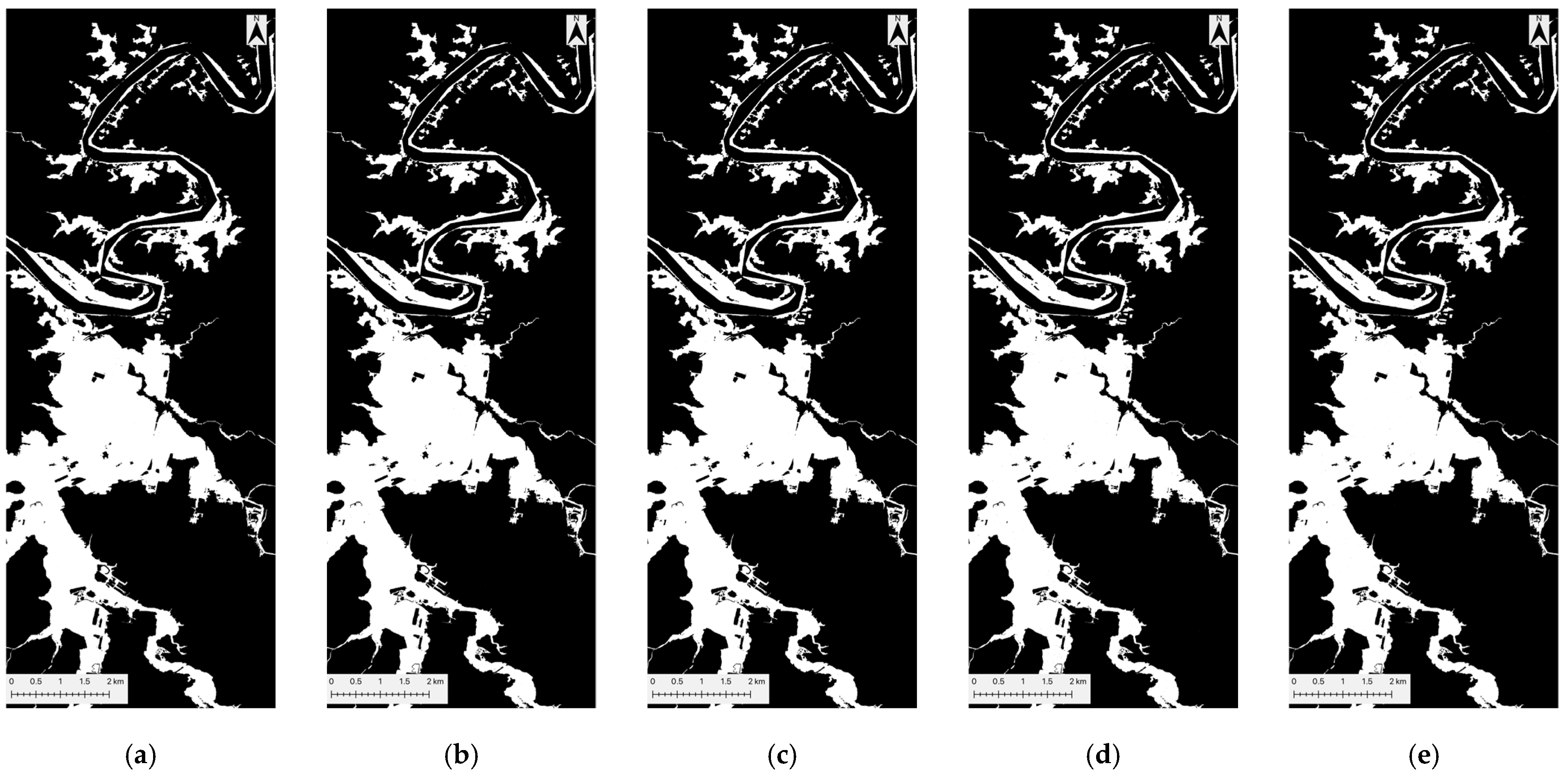
Figure 8.
DT flood prediction maps for five datasets: (a) peak-flood image, (b) CA-dNDWI, (c) CA-cNDWI, (d) CA-NDII, and (e) CA-NDWI. Each sub-figure delineates inundated water (white) from non-inundated areas (black), which include both permanent water and non-water areas.
Figure 8.
DT flood prediction maps for five datasets: (a) peak-flood image, (b) CA-dNDWI, (c) CA-cNDWI, (d) CA-NDII, and (e) CA-NDWI. Each sub-figure delineates inundated water (white) from non-inundated areas (black), which include both permanent water and non-water areas.
Figure 9.
RF flood prediction maps for five datasets: (a) peak-flood image, (b) CA-dNDWI, (c) CA-cNDWI, (d) CA-NDII, and (e) CA-NDWI. Each sub-figure delineates inundated water (white) from non-inundated areas (black), which include both permanent water and non-water areas.
Figure 9.
RF flood prediction maps for five datasets: (a) peak-flood image, (b) CA-dNDWI, (c) CA-cNDWI, (d) CA-NDII, and (e) CA-NDWI. Each sub-figure delineates inundated water (white) from non-inundated areas (black), which include both permanent water and non-water areas.
Figure 10.
EM flood prediction maps for five datasets: (a) peak-flood image, (b) CA-dNDWI, (c) CA-cNDWI, (d) CA-NDII, and (e) CA-NDWI. Each sub-figure delineates inundated water (white) from non-inundated areas (black), which include both permanent water and non-water areas.
Figure 10.
EM flood prediction maps for five datasets: (a) peak-flood image, (b) CA-dNDWI, (c) CA-cNDWI, (d) CA-NDII, and (e) CA-NDWI. Each sub-figure delineates inundated water (white) from non-inundated areas (black), which include both permanent water and non-water areas.
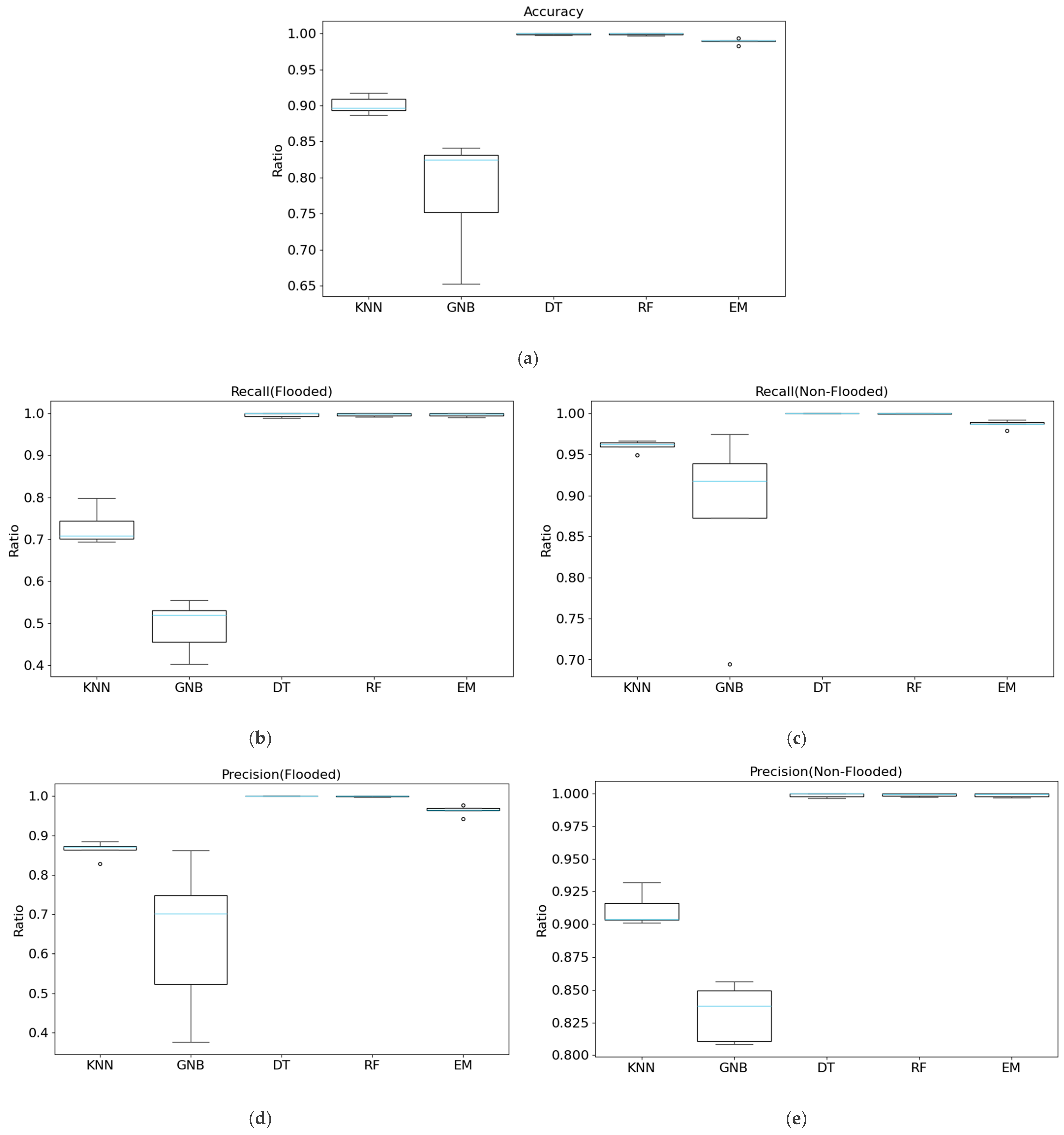
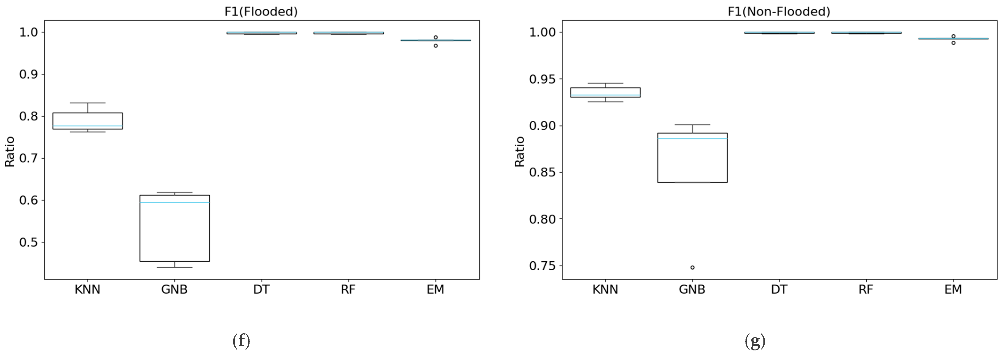
Figure 11.
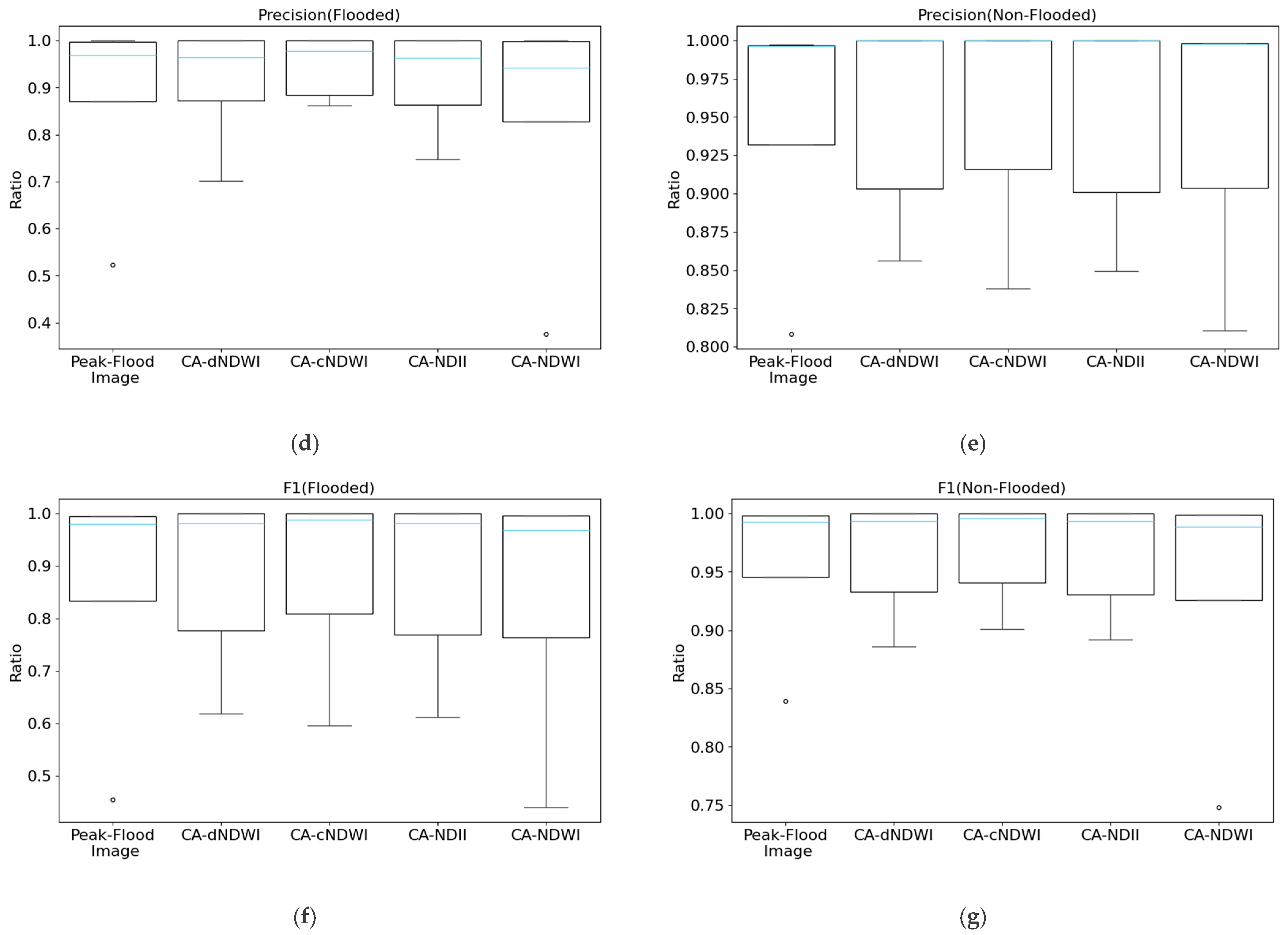
Boxplots of effectiveness metrics for each model (KNN, GNB, DT, RF, EM) across five datasets (the peak-image flood, CA-dNDWI, CA-cNDWI, CA-NDII, CA-NDWI: (a) accuracy; (b) recall (flooded); (c) recall (non-flooded); (d) precision (flooded); (e) precision (non-flooded); (f) F1 (flooded); and (g) F1 (non-flooded). The sky-blue line represents the median value across the five datasets for each model, while blank circles indicate outliers.
Figure 11.
Boxplots of effectiveness metrics for each model (KNN, GNB, DT, RF, EM) across five datasets (the peak-image flood, CA-dNDWI, CA-cNDWI, CA-NDII, CA-NDWI: (a) accuracy; (b) recall (flooded); (c) recall (non-flooded); (d) precision (flooded); (e) precision (non-flooded); (f) F1 (flooded); and (g) F1 (non-flooded). The sky-blue line represents the median value across the five datasets for each model, while blank circles indicate outliers.
Figure 12.
Boxplots of efficiency metrics for each model (KNN, GNB, DT, RF, EM) across five datasets (the peak-image flood, CA-dNDWI, CA-cNDWI, CA-NDII, CA-NDWI: (a) training time; (b) testing time; (c) training memory usage; and (d) testing memory usage. The sky-blue line represents the median value across the five datasets for each model, while blank circles indicate outliers.
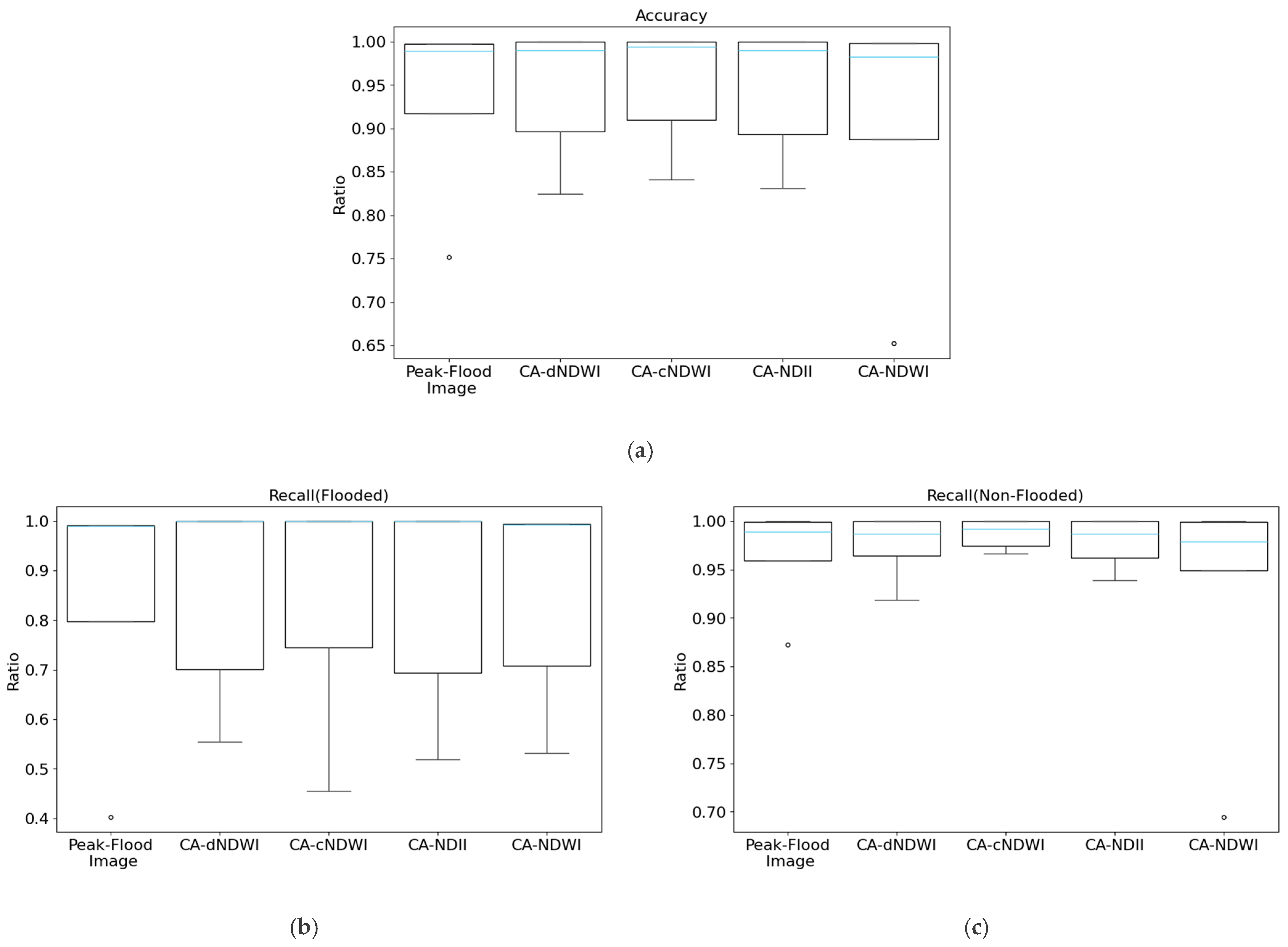
Figure 13.
Boxplots of effectiveness metrics for each dataset (the peak-image flood, CA-dNDWI, CA-cNDWI, CA-NDII, CA-NDWI) across five models (KNN, GNB, DT, RF, EM): (a) accuracy; (b) recall (flooded); (c) recall (non-flooded); (d) precision (flooded); (e) precision (non-flooded); (f) F1 (flooded); and (g) F1 (non-flooded). The sky-blue line represents the median value across the five models for each dataset, while blank circles indicate outliers.
Figure 14.
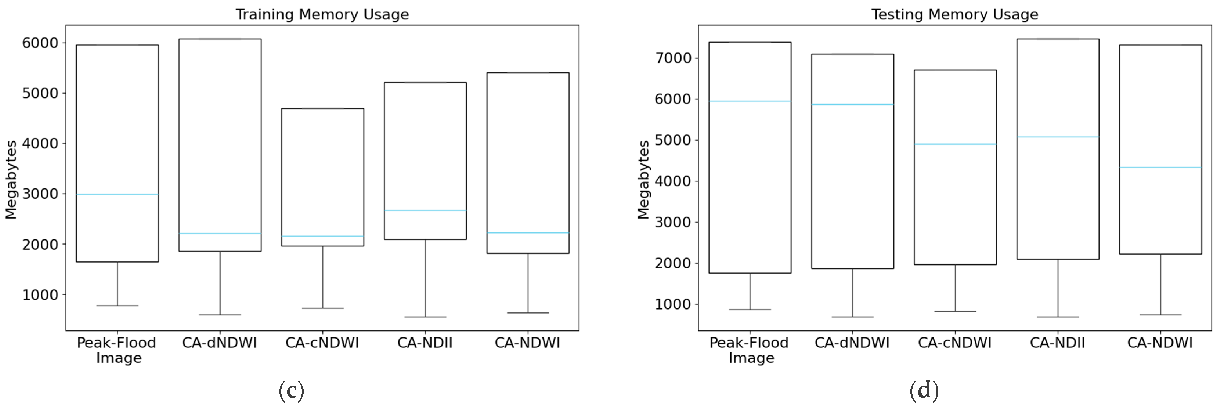
Boxplots of efficiency metrics for each dataset (the peak-image flood, CA-dNDWI, CA-cNDWI, CA-NDII, CA-NDWI) across five models (KNN, GNB, DT, RF, EM): (a) training time; (b) testing time; (c) training memory usage; and (d) testing memory usage. The sky-blue line represents the median value across the five models for each dataset, while blank circles indicate outliers.
Figure 14.
Boxplots of efficiency metrics for each dataset (the peak-image flood, CA-dNDWI, CA-cNDWI, CA-NDII, CA-NDWI) across five models (KNN, GNB, DT, RF, EM): (a) training time; (b) testing time; (c) training memory usage; and (d) testing memory usage. The sky-blue line represents the median value across the five models for each dataset, while blank circles indicate outliers.
Table 1.
Spectral Bands of PlanetScope Imagery.
Table 1.
Spectral Bands of PlanetScope Imagery.
| Order | Band | Type | Wavelength (nm) |
|---|
| 1 | Blue (B) | Visible | 455–515 |
| 2 | Green (G) | Visible | 500–590 |
| 3 | Red (R) | Visible | 590–670 |
| 4 | Near-infrared (NIR) | Invisible | 780–860 |
Table 2.
Characteristics of the pre-processed labeled image.
Table 2.
Characteristics of the pre-processed labeled image.
| Parameter | Value |
|---|
| Width | 1184 pixels |
| Height | 3081 pixels |
| Inundated Regions | 25.71% (938,033 pixels) |
| Non-Inundated Regions | 74.29% (2,709,871 pixels) |
| Spatial Pixel Size (Width × Height) | 4.65 × 5.25 m |
| Image Size (Width × Height) | 5.51 × 16.18 km |
Table 3.
Summary of effectiveness metrics for five baselines (spectral indices with pre-defined thresholds). Bold values highlight the maximum score for each metric.
Table 3.
Summary of effectiveness metrics for five baselines (spectral indices with pre-defined thresholds). Bold values highlight the maximum score for each metric.
| Baseline | Threshold | Accuracy | Recall (Flooded) | Recall (Non-Flooded) | Precision (Flooded) | Precision (Non-Flooded) | F1 (Flooded) | F1
(Non-Flooded) |
|---|
| NDWIpeak-flood | 0.2 | 0.692 | 0.429 | 0.784 | 0.407 | 0.798 | 0.418 | 0.791 |
| NDWIpeak-flood | 0.3 | 0.763 | 0.149 | 0.976 | 0.686 | 0.768 | 0.244 | 0.860 |
| NDII | 0.1 | 0.833 | 0.506 | 0.946 | 0.766 | 0.847 | 0.609 | 0.894 |
| cNDWI | 0.1 | 0.587 | 0.243 | 0.706 | 0.222 | 0.729 | 0.232 | 0.717 |
| dNDWI | 0.2 | 0.794 | 0.639 | 0.848 | 0.593 | 0.871 | 0.615 | 0.860 |
Table 4.
The mean and standard deviation for the effectiveness metrics. The mean value for each of the metrics is close to 1, indicating that most of the approaches performed strongly.
Table 4.
The mean and standard deviation for the effectiveness metrics. The mean value for each of the metrics is close to 1, indicating that most of the approaches performed strongly.
| Metric | Accuracy | Recall (Flooded) | Recall (Non-Flooded) | Precision (Flooded) | Precision (Non-Flooded) | F1 (Flooded) | F1
(Non-Flooded) |
|---|
| Mean | 0.934 | 0.842 | 0.965 | 0.894 | 0.948 | 0.862 | 0.956 |
| Standard Deviation | 0.093 | 0.210 | 0.644 | 0.160 | 0.069 | 0.184 | 0.064 |
Table 5.
Summary of effectiveness metrics for model-dataset combinations. Values significantly lower than the mean are marked with daggers (†). The number of symbols corresponds to the number of standard deviations below the mean. No values are significantly higher than the mean.
Table 5.
Summary of effectiveness metrics for model-dataset combinations. Values significantly lower than the mean are marked with daggers (†). The number of symbols corresponds to the number of standard deviations below the mean. No values are significantly higher than the mean.
| Model | Dataset | Accuracy | Recall (Flooded) | Recall (Non-Flooded) | Precision (Flooded) | Precision (Non-Flooded) | F1 (Flooded) | F1 (Non-Flooded) |
|---|
| KNN | Peak-Flood Image | 0.918 | 0.798 | 0.959 | 0.871 | 0.932 | 0.833 | 0.945 |
| CA-dNDWI | 0.897 | 0.701 | 0.965 | 0.873 | 0.903 | 0.778 | 0.933 |
| CA-cNDWI | 0.909 | 0.745 | 0.966 | 0.885 | 0.916 | 0.809 | 0.941 |
| CA-NDII | 0.893 | 0.694 | 0.962 | 0.864 | 0.901 | 0.770 | 0.930 |
| CA-NDWI | 0.887 | 0.709 | 0.949 | 0.828 | 0.904 | 0.764 | 0.926 |
| GNB | Peak-Flood Image | 0.752 † | 0.402 ††† | 0.873 † | 0.523 ††† | 0.808 ††† | 0.455 ††† | 0.839 † |
| CA-dNDWI | 0.825 † | 0.555 † | 0.918 | 0.702 † | 0.856 † | 0.619 † | 0.886 † |
| CA-cNDWI | 0.841 | 0.455 † | 0.975 | 0.862 | 0.838 † | 0.596 | 0.901 |
| CA-NDII | 0.831 † | 0.519 † | 0.939 | 0.747 | 0.849 † | 0.613 † | 0.892 † |
| CA-NDWI | 0.652 ††† | 0.531 † | 0.694 ††† | 0.376 ††† | 0.810 † | 0.440 ††† | 0.748 ††† |
| DT | Peak-Flood Image | 0.997 | 0.989 | 1.000 | 1.000 | 0.996 | 0.995 | 0.998 |
| CA-dNDWI | 1.000 | 1.000 | 1.000 | 1.000 | 1.000 | 1.000 | 1.000 |
| CA-cNDWI | 1.000 | 1.000 | 1.000 | 1.000 | 1.000 | 1.000 | 1.000 |
| CA-NDII | 1.000 | 0.999 | 1.000 | 1.000 | 1.000 | 1.000 | 1.000 |
| CA-NDWI | 0.998 | 0.993 | 1.000 | 1.000 | 0.998 | 0.996 | 0.999 |
| RF | Peak-Flood Image | 0.997 | 0.991 | 0.999 | 0.998 | 0.997 | 0.995 | 0.998 |
| CA-dNDWI | 1.000 | 0.999 | 1.000 | 1.000 | 1.000 | 1.000 | 1.000 |
| CA-cNDWI | 1.000 | 1.000 | 1.000 | 1.000 | 1.000 | 1.000 | 1.000 |
| CA-NDII | 1.000 | 0.999 | 1.000 | 1.000 | 1.000 | 1.000 | 1.000 |
| CA-NDWI | 0.998 | 0.994 | 0.999 | 0.998 | 0.998 | 0.996 | 0.999 |
| EM | Peak-Flood Image | 0.989 | 0.991 | 0.989 | 0.969 | 0.997 | 0.980 | 0.993 |
| CA-dNDWI | 0.990 | 0.999 | 0.987 | 0.964 | 1.000 | 0.982 | 0.993 |
| CA-cNDWI | 0.994 | 1.000 | 0.992 | 0.977 | 1.000 | 0.988 | 0.996 |
| CA-NDII | 0.990 | 0.999 | 0.987 | 0.964 | 1.000 | 0.981 | 0.993 |
| CA-NDWI | 0.983 | 0.994 | 0.979 | 0.943 | 0.998 | 0.968 | 0.988 |
Table 6.
The mean and standard deviation for the efficiency metrics. The mean training time is larger than the mean testing time.
Table 6.
The mean and standard deviation for the efficiency metrics. The mean training time is larger than the mean testing time.
| Metric | Training Time (s) | Testing Time (s) | Training Memory Usage (MB) | Testing Memory Usage (MB) |
|---|
| Mean | 1337.935 | 27.655 | 3186.419 | 4475.821 |
| Standard Deviation | 1575.478 | 55.105 | 5212.443 | 7212.900 |
Table 7.
Summary of efficiency metrics for model-dataset combinations. Values significantly different from the mean are marked with two symbols: asterisks (*) for higher values and daggers (†) for lower values. The number of symbols corresponds to the number of standard deviations above or below the mean.
| Model | Dataset | Training Time (s) | Testing Time (s) | Training Memory (MB) | Testing Memory Usage (MB) |
|---|
| KNN | Peak-Flood Image | 64.837 | 48.614 | 5955.547 * | 5948.859 |
| CA-dNDWI | 61.188 | 46.350 | 6079.125 * | 5869.203 |
| CA-cNDWI | 72.040 | 50.509 | 4697.828 | 4896.906 |
| CA-NDII | 59.614 | 44.955 | 5212.016 | 5080.719 |
| CA-NDWI | 60.689 | 45.508 | 5405.656 * | 4333.297 |
| GNB | Peak-Flood Image | 4.183 | 0.113 † | 1652.484 | 1749.891 |
| CA-dNDWI | 4.176 | 0.230 | 1864.734 | 1864.734 |
| CA-cNDWI | 5.059 | 0.278 | 1965.203 | 1972.578 |
| CA-NDII | 4.215 | 0.227 | 2099.375 | 2099.375 |
| CA-NDWI | 4.246 | 0.258 | 2220.703 | 2221.359 |
| DT | Peak-Flood Image | 190.609 | 1.013 | 779.844 † | 875.516 † |
| CA-dNDWI | 676.742 | 1.338 | 597.297 † | 700.250 † |
| CA-cNDWI | 832.863 | 0.961 | 730.516 † | 826.188 † |
| CA-NDII | 477.909 | 1.076 | 555.609 † | 691.375 † |
| CA-NDWI | 696.648 | 1.254 | 634.875 † | 741.938 † |
| RF | Peak-Flood Image | 1101.444 | 18.546 | 2985.891 | 7391.078 * |
| CA-dNDWI | 3601.179 * | 22.033 | 2215.188 | 7103.000 |
| CA-cNDWI | 2363.282 | 20.116 | 2158.156 | 6716.516 |
| CA-NDII | 2949.289 * | 20.711 | 2674.641 | 7469.406 * |
| CA-NDWI | 3493.978 * | 21.585 | 1825.625 | 7331.672 * |
| EM | Peak-Flood Image | 1361.073 | 68.287 * | 5955.547 * | 7391.078 * |
| CA-dNDWI | 4343.285 * | 69.958 * | 6079.125 * | 7103.000 |
| CA-cNDWI | 3273.243 * | 71.864 * | 4697.828 | 6716.516 |
| CA-NDII | 3491.026 * | 66.968 * | 5212.016 | 7469.406 |
| CA-NDWI | 4255.560 * | 68.606 * | 5405.656 * | 7331.672 * |
Table 8.
Summary of p-values from one-way ANOVA for five models across five datasets, using the effectiveness metrics.
Table 8.
Summary of p-values from one-way ANOVA for five models across five datasets, using the effectiveness metrics.
| Effectiveness Metrics | p-Value |
|---|
|
Accuracy
|
9.7880 × 10⁻⁹ |
|
Recall (Flooded)
|
2.8140 × 10⁻¹⁶ |
|
Recall (Non-Flooded)
|
4.8080 × 10⁻³ |
|
Precision (Flooded)
|
7.3880 × 10⁻⁶ |
|
Precision (Non-Flooded)
|
4.5810 × 10⁻¹⁶ |
|
F1 (Flooded)
|
2.5020 × 10⁻¹³ |
|
F1 (Non-Flooded)
|
1.8440 × 10⁻⁷ |
Table 9.
Pairwise model comparisons of p-adj values calculated by Tukey’s HSD for the accuracy. Bold values indicate a significantly different pair (p-adj value ≤ 0.05). The grey cells indicate the placeholders.
Table 9.
Pairwise model comparisons of p-adj values calculated by Tukey’s HSD for the accuracy. Bold values indicate a significantly different pair (p-adj value ≤ 0.05). The grey cells indicate the placeholders.
| Models | KNN | GNB | DT | RF | EM |
|---|
| KNN | | | | | |
| GNB | 0.0003 | | | | |
| DT | 0.0029 | <0.0001 | | | |
| RF | 0.0029 | <0.0001 | 1.0000 | | |
| EM | 0.0075 | <0.0001 | 0.9928 | 0.9929 | |
Table 10.
Pairwise model comparisons of p-adj values calculated by Tukey’s HSD for recall (flood-ed/non-flooded). Bold values indicate a significantly different pair (p-adj value ≤ 0.05). The grey cells indicate the dividers for the two metrics.
Table 10.
Pairwise model comparisons of p-adj values calculated by Tukey’s HSD for recall (flood-ed/non-flooded). Bold values indicate a significantly different pair (p-adj value ≤ 0.05). The grey cells indicate the dividers for the two metrics.
| Models | KNN | GNB | DT | RF | EM | |
|---|
| KNN | | 0.1138 | 0.7097 | 0.7149 | 0.9108 | Recall (Non-Flooded) |
| GNB | <0.0001 | | 0.0079 | 0.0081 | 0.0201 |
| DT | <0.0001 | <0.0001 | | 1.0000 | 0.9929 |
| RF | <0.0001 | <0.0001 | 1.0000 | | 0.9934 |
| EM | <0.0001 | <0.0001 | 1.0000 | 1.0000 | | |
| | Recall (Flooded) | | |
Table 11.
Pairwise model comparisons of p-adj values calculated by Tukey’s HSD for precision (flooded/non-flooded). Bold values indicate a significantly different pair (p-adj value ≤ 0.05). The grey cells indicate the dividers for the two metrics.
Table 11.
Pairwise model comparisons of p-adj values calculated by Tukey’s HSD for precision (flooded/non-flooded). Bold values indicate a significantly different pair (p-adj value ≤ 0.05). The grey cells indicate the dividers for the two metrics.
| Models | KNN | GNB | DT | RF | EM | |
|---|
| KNN | | <0.0001 | <0.0001 | <0.0001 | <0.0001 | Precision (Non-Flooded) |
| GNB | 0.0051 | | <0.0001 | <0.0001 | <0.0001 |
| DT | 0.1361 | <0.0001 | | 1.0000 | 1.0000 |
| RF | 0.1398 | <0.0001 | 1.0000 | | 1.0000 |
| EM | 0.3958 | 0.0001 | 0.9612 | 0.9642 | | |
| | Precision (Flooded) | | |
Table 12.
Pairwise model comparisons of p-adj values calculated by Tukey’s HSD for F1 (flooded/non-flooded). Bold values indicate a significantly different pair (p-adj value ≤ 0.05). The grey cells indicate the dividers for the two metrics.
Table 12.
Pairwise model comparisons of p-adj values calculated by Tukey’s HSD for F1 (flooded/non-flooded). Bold values indicate a significantly different pair (p-adj value ≤ 0.05). The grey cells indicate the dividers for the two metrics.
| Models | KNN | GNB | DT | RF | EM | |
|---|
| KNN | | 0.0018 | 0.0154 | 0.0155 | 0.0335 | F1 (Non-Flooded) |
| GNB | 0.0001 | | <0.0001 | <0.0001 | <0.0001 |
| DT | <0.0001 | <0.0001 | | 1.0000 | 0.996 |
| RF | <0.0001 | <0.0001 | 1.0000 | | 0.9961 |
| EM | <0.0001 | <0.0001 | 0.9564 | 0.9570 | | |
| | F1 (Flooded) | | |
Table 13.
Summary of p-values from one-way ANOVA for five models across five datasets, using the efficiency metrics.
Table 13.
Summary of p-values from one-way ANOVA for five models across five datasets, using the efficiency metrics.
| Efficiency Metrics | p-Value |
|---|
|
Training Time
|
2.0320 × 10⁻⁷ |
|
Testing Time
|
1.0000 × 10⁻²⁵ |
|
Training Memory Usage
|
4.6500 × 10⁻¹⁴ |
|
Testing Memory Usage
|
8.0690 × 10⁻¹⁸ |
Table 14.
Pairwise model comparisons of p-adj values calculated by Tukey’s HSD for training/testing time. Bold values indicate a significantly different pair (p-adj value ≤ 0.05). The grey cells indicate the dividers for the two metrics.
Table 14.
Pairwise model comparisons of p-adj values calculated by Tukey’s HSD for training/testing time. Bold values indicate a significantly different pair (p-adj value ≤ 0.05). The grey cells indicate the dividers for the two metrics.
| Models | KNN | GNB | DT | RF | EM | |
|---|
| KNN | | <0.0001 | <0.0001 | <0.0001 | <0.0001 | Testing Time |
| GNB | 0.9999 | | 0.8624 | <0.0001 | <0.0001 |
| DT | 0.7883 | 0.7159 | | <0.0001 | <0.0001 |
| RF | 0.0001 | 0.0001 | 0.0011 | | <0.0001 |
| EM | <0.0001 | <0.0001 | <0.0001 | 0.6208 | | |
| | Training Time | | |
Table 15.
Pairwise model comparisons of p-adj values calculated by Tukey’s HSD for training/testing memory usage. Bold values indicate a significantly different pair (p-adj value ≤ 0.05). The grey cells indicate the dividers for the two metrics.
Table 15.
Pairwise model comparisons of p-adj values calculated by Tukey’s HSD for training/testing memory usage. Bold values indicate a significantly different pair (p-adj value ≤ 0.05). The grey cells indicate the dividers for the two metrics.
| Models | KNN | GNB | DT | RF | EM | |
|---|
| KNN | | <0.0001 | <0.0001 | <0.0001 | <0.0001 | Testing Memory
Usage |
| GNB | <0.0001 | | 0.0004 | <0.0001 | <0.0001 |
| DT | <0.0001 | 0.0008 | | <0.0001 | <0.0001 |
| RF | <0.0001 | 0.5555 | <0.0001 | | 1.0000 |
| EM | 1.0000 | <0.0001 | <0.0001 | <0.0001 | | |
| | Training | | |
Table 16.
Summary of p-values from one-way ANOVA for five datasets evaluated by five models separately, using effectiveness metrics.
Table 16.
Summary of p-values from one-way ANOVA for five datasets evaluated by five models separately, using effectiveness metrics.
| Effectiveness Metrics | p-Value |
|---|
|
Accuracy
| 0.9550 |
|
Recall (Flooded)
| 0.9990 |
|
Recall (Non-Flooded)
| 0.6190 |
|
Precision (Flooded)
| 0.8420 |
|
Precision (Non-Flooded)
| 0.9990 |
|
F1 (Flooded)
| 0.9950 |
|
F1 (Non-Flooded)
| 0.9260 |
Table 17.
Pairwise dataset comparisons of p-adj values calculated by Tukey’s HSD for accuracy. The grey cells indicate the placeholders.
Table 17.
Pairwise dataset comparisons of p-adj values calculated by Tukey’s HSD for accuracy. The grey cells indicate the placeholders.
| Datasets | Peak-Flood
Image | CA-dNDWI | CA-cNDWI | CA-NDII | CA-NDWI |
|---|
Peak-Flood
Image | | | | | |
| CA-dNDWI | 0.9997 | | | | |
| CA-cNDWI | 0.9984 | 1.0000 | | | |
| CA-NDII | 0.9997 | 1.0000 | 1.0000 | | |
| CA-NDWI | 0.9927 | 0.9721 | 0.9516 | 0.9709 | |
Table 18.
Pairwise dataset comparisons of p-adj values calculated by Tukey’s HSD for recall (flooded/non-flooded). The grey cells indicate the dividers for the two metrics.
Table 18.
Pairwise dataset comparisons of p-adj values calculated by Tukey’s HSD for recall (flooded/non-flooded). The grey cells indicate the dividers for the two metrics.
| Datasets | Peak-Flood
Image | CA-dNDWI | CA-cNDWI | CA-NDII | CA-NDWI | |
|---|
Peak-Flood
Image | | 0.9992 | 0.9821 | 0.9974 | 0.8753 | Recall (Non-Flooded) |
| CA-dNDWI | 1.0000 | | 0.9981 | 1.0000 | 0.7599 |
| CA-cNDWI | 1.0000 | 1.0000 | | 0.9995 | 0.5830 |
| CA-NDII | 1.0000 | 1.0000 | 1.0000 | | 0.7113 |
| CA-NDWI | 1.0000 | 1.0000 | 1.0000 | 1.0000 | | |
| | Recall (Flooded) | |
Table 19.
Pairwise dataset comparisons of p-adj values calculated by Tukey’s HSD for precision (flooded/non-flooded). The grey cells indicate the dividers for the two metrics.
Table 19.
Pairwise dataset comparisons of p-adj values calculated by Tukey’s HSD for precision (flooded/non-flooded). The grey cells indicate the dividers for the two metrics.
| Datasets | Peak-Flood
Image | CA-dNDWI | CA-cNDWI | CA-NDII | CA-NDWI | |
|---|
Peak-Flood
Image | | 0.9999 | 1.0000 | 1.0000 | 1.0000 | Precision (Non-Flooded) |
| CA-dNDWI | 0.9971 | | 1.0000 | 1.0000 | 0.9995 |
| CA-cNDWI | 0.9582 | 0.9966 | | 1.0000 | 0.9997 |
| CA-NDII | 0.9941 | 1.0000 | 0.9985 | | 0.9998 |
| CA-NDWI | 0.9939 | 0.9448 | 0.8115 | 0.9258 | | |
| | Precision (Flooded) | |
Table 20.
Pairwise dataset comparisons of p-adj values calculated by Tukey’s HSD for F1 (flooded/non-flooded). The grey cells indicate the dividers for the two metrics.
Table 20.
Pairwise dataset comparisons of p-adj values calculated by Tukey’s HSD for F1 (flooded/non-flooded). The grey cells indicate the dividers for the two metrics.
| Datasets | Peak-Flood
Image | CA-dNDWI | CA-cNDWI | CA-NDII | CA-NDWI | |
|---|
Peak-Flood
Image | | 0.9997 | 0.9982 | 0.9997 | 0.9833 | F1
(Non-Flooded) |
| CA-dNDWI | 0.9997 | | 1.0000 | 1.0000 | 0.9523 |
| CA-cNDWI | 0.9995 | 1.0000 | | 1.0000 | 0.9199 |
| CA-NDII | 0.9998 | 1.0000 | 1.0000 | | 0.9487 |
| CA-NDWI | 0.9999 | 0.9970 | 0.9962 | 0.9978 | | |
| | F1 (Flooded) | |
Table 21.
Summary of p-values from one-way ANOVA for five datasets evaluated by five models separately, using effectiveness metrics.
Table 21.
Summary of p-values from one-way ANOVA for five datasets evaluated by five models separately, using effectiveness metrics.
| Efficiency Metrics | p-Value |
|---|
|
Training Time
| 0.7910 |
|
Testing Time
| 0.9990 |
|
Training Memory Usage
| 0.9920 |
|
Testing Memory Usage
| 0.9990 |
Table 22.
Pairwise dataset comparisons of p-adj values calculated by Tukey’s HSD for training/testing time. The grey cells indicate the dividers for the two metrics.
Table 22.
Pairwise dataset comparisons of p-adj values calculated by Tukey’s HSD for training/testing time. The grey cells indicate the dividers for the two metrics.
| Datasets | Peak-Flood
Image | CA-dNDWI | CA-cNDWI | CA-NDII | CA-NDWI | |
|---|
Peak-Flood
Image | | 1.0000 | 1.0000 | 1.0000 | 1.0000 | Testing Time |
| CA-dNDWI | 0.7849 | | 1.0000 | 1.0000 | 1.0000 |
| CA-cNDWI | 0.9470 | 0.9937 | | 1.0000 | 1.0000 |
| CA-NDII | 0.9236 | 0.9974 | 1.0000 | | 1.0000 |
| CA-NDWI | 0.8022 | 1.0000 | 0.9954 | 0.9983 | | |
| | Training Time | |
Table 23.
Pairwise dataset comparisons of p-adj values calculated by Tukey’s HSD for training/testing memory usage. The grey cells indicate the dividers for the two metrics.
Table 23.
Pairwise dataset comparisons of p-adj values calculated by Tukey’s HSD for training/testing memory usage. The grey cells indicate the dividers for the two metrics.
| Datasets | Peak-Flood
Image | CA-dNDWI | CA-cNDWI | CA-NDII | CA-NDWI | |
|---|
Peak-Flood
Image | | 1.0000 | 0.9993 | 1.0000 | 0.9999 | Testing Memory
Usage |
| CA-dNDWI | 1.0000 | | 0.9998 | 1.0000 | 1.0000 |
| CA-cNDWI | 0.9915 | 0.9956 | | 0.9998 | 1.0000 |
| CA-NDII | 0.9994 | 0.9999 | 0.9995 | | 1.0000 |
| CA-NDWI | 0.9988 | 0.9997 | 0.9998 | 1.0000 | | |
| | Training
Memory Usage | |
Table 24.
The mean and standard deviation of the differences in the effectiveness metrics between the CA datasets and the peak-flood image. The mean value for each of the metrics is small, indicating that there is not much difference between the datasets.
Table 24.
The mean and standard deviation of the differences in the effectiveness metrics between the CA datasets and the peak-flood image. The mean value for each of the metrics is small, indicating that there is not much difference between the datasets.
| Metric | Accuracy | Recall (Flooded) | Recall (Non-Flooded) | Precision (Flooded) | Precision (Non-Flooded) | F1 (Flooded) | F1
(Non-Flooded) |
|---|
| Mean | 0.004 | 0.010 | 0.002 | 0.027 | 0.003 | 0.003 | 0.013 |
| Standard Deviation | 0.041 | 0.674 | 0.051 | 0.104 | 0.020 | 0.020 | 0.065 |
Table 25.
Summary of differences in the effectiveness metrics of the comparison of the CA datasets with the peak-flood image for all model-dataset combinations. For each metric, the mean and standard deviation were calculated. Values significantly different from the mean are marked with two symbols: asterisks (*) for higher values and daggers (†) for lower values. The number of symbols corresponds to the number of standard deviations above or below the mean.
| Model | Dataset | Accuracy | Recall (Flooded) | Recall (Non-Flooded) | Precision (Flooded) | Precision (Non-Flooded) | F1 (Flooded) | F1
(Non-Flooded) |
|---|
| KNN | CA-dNDWI | −0.021 | −0.097 † | 0.006 | 0.002 | −0.029 † | −0.055 | −0.012 |
| CA-cNDWI | −0.009 | −0.053 | 0.007 | 0.014 | −0.016 | −0.024 | −0.004 |
| CA-NDII | −0.025 | −0.104 † | 0.003 | −0.007 | −0.031 † | −0.063 | −0.015 |
| CA-NDWI | −0.031 | −0.089 † | −0.010 | −0.043 | −0.028 † | −0.069 † | −0.019 |
| GNB | CA-dNDWI | 0.073 * | 0.153 ** | 0.045 | 0.179 * | 0.048 ** | 0.164 ** | 0.047 * |
| CA-cNDWI | 0.089 ** | 0.053 | 0.102 ** | 0.339 ** | 0.030 * | 0.141 ** | 0.062 ** |
| CA-NDII | 0.079 * | 0.117 * | 0.066 * | 0.224 * | 0.041 ** | 0.158 ** | 0.053 * |
| CA-NDWI | −0.100 † | 0.129 * | −0.179 † | −0.147 † | 0.002 | −0.015 | −0.091 †† |
| DT | CA-dNDWI | 0.003 | 0.011 | 0.000 | 0.000 | 0.004 | 0.005 | 0.002 |
| CA-cNDWI | 0.003 | 0.011 | 0.000 | 0.000 | 0.004 | 0.005 | 0.002 |
| CA-NDII | 0.003 | 0.010 | 0.000 | 0.000 | 0.004 | 0.005 | 0.002 |
| CA-NDWI | 0.001 | 0.004 | 0.000 | 0.000 | 0.002 | 0.001 | 0.001 |
| RF | CA-dNDWI | 0.003 | 0.008 | 0.001 | 0.002 | 0.003 | 0.005 | 0.002 |
| CA-cNDWI | 0.003 | 0.009 | 0.001 | 0.002 | 0.003 | 0.005 | 0.002 |
| CA-NDII | 0.003 | 0.008 | 0.001 | 0.002 | 0.003 | 0.005 | 0.002 |
| CA-NDWI | 0.001 | 0.003 | 0.000 | 0.000 | 0.001 | 0.001 | 0.001 |
| EM | CA-dNDWI | 0.001 | 0.008 | −0.002 | −0.005 | 0.003 | 0.002 | 0.000 |
| CA-cNDWI | 0.005 | 0.009 | 0.003 | 0.008 | 0.003 | 0.008 | 0.003 |
| CA-NDII | 0.001 | 0.008 | −0.002 | −0.005 | 0.003 | 0.001 | 0.000 |
| CA-NDWI | −0.006 | 0.003 | −0.010 | −0.026 | 0.001 | −0.012 | −0.005 |
Table 26.
Summary of the paired two-tailed t-test results comparing the peak-flood image with the CA datasets across the effectiveness metrics. Each evaluation was conducted separately for each model. Values with a significant difference are in bold.
Table 26.
Summary of the paired two-tailed t-test results comparing the peak-flood image with the CA datasets across the effectiveness metrics. Each evaluation was conducted separately for each model. Values with a significant difference are in bold.
| Model | Accuracy | Recall (Flooded) | Recall (Non-Flooded) | Precision (Flooded) | Precision (Non-Flooded) | F1 (Flooded) | F1 (Non-Flooded) |
|---|
| KNN | 0.019 | 0.005 | 0.728 | 0.539 | 0.005 | 0.013 | 0.029 |
| GNB | 0.492 | 0.013 | 0.902 | 0.249 | 0.058 | 0.078 | 0.659 |
| DT | 0.015 | 0.013 | N/A | N/A | 0.006 | 0.028 | 0.006 |
| RF | 0.015 | 0.014 | 0.058 | 0.058 | 0.015 | 0.028 | 0.006 |
| EM | 0.920 | 0.014 | 0.382 | 0.393 | 0.015 | 0.956 | 0.783 |
Table 27.
The mean and standard deviation of the efficiency metrics. There is a wide range in this table since the metrics use different measures and are on a wide scale.
Table 27.
The mean and standard deviation of the efficiency metrics. There is a wide range in this table since the metrics use different measures and are on a wide scale.
| Metric | Training Time (s) | Testing Time (s) | Training Memory (MB) | Testing Memory (MB) |
|---|
| Mean | 991.882 | 0.010 | −249.304 | −244.329 |
| Standard Deviation | 1118.160 | 0.067 | 560.034 | 506.287 |
Table 28.
Summary of differences in the efficiency metrics compared with the peak-flood image for all model-dataset combinations. For each metric, the mean and standard deviation were calculated. Values significantly different from the mean are marked with two symbols: asterisks (*) for higher values and daggers (†) for lower values. The number of symbols corresponds to the number of standard deviations above or below the mean.
| Model | Dataset | Training Time (s) | Testing Time (s) | Training Memory Usage (MB) | Testing Memory Usage (MB) |
|---|
| KNN | CA-dNDWI | −3.649 | −0.097 † | 123.578 | −79.656 |
| CA-cNDWI | 7.203 | −0.053 | −1257.719 † | −1051.953 †† |
| CA-NDII | −5.223 | −0.104 † | −743.531 † | −868.14 † |
| CA-NDWI | −4.148 | −0.089 † | −549.891 | −1615.562 ††† |
| GNB | CA-dNDWI | −0.007 | 0.153 ** | 212.250 | 114.843 |
| CA-cNDWI | 0.876 | 0.053 | 312.719 | 222.687 |
| CA-NDII | 0.032 | 0.117 * | 446.891 | 349.484 |
| CA-NDWI | 0.063 | 0.129 * | 568.219 * | 471.468 |
| DT | CA-dNDWI | 486.133 | 0.011 | −182.547 | −175.266 |
| CA-cNDWI | 642.254 | 0.011 | −49.328 | −49.328 |
| CA-NDII | 287.300 | 0.010 | −224.235 | −184.141 |
| CA-NDWI | 506.039 | 0.004 | −144.969 | −133.578 |
| RF | CA-dNDWI | 2499.735 ** | 0.008 | −770.703 † | −288.078 |
| CA-cNDWI | 1261.838 * | 0.009 | −827.735 † | −674.562 † |
| CA-NDII | 1847.845 * | 0.008 | −311.250 | 78.328 |
| CA-NDWI | 2392.534 ** | 0.003 | −1160.266 †† | −59.406 |
| EM | CA-dNDWI | 2982.212 ** | 0.008 | 123.578 | −288.078 |
| CA-cNDWI | 1912.17 * | 0.009 | −1257.719 †† | −674.562 † |
| CA-NDII | 2129.953 * | 0.008 | −743.531 † | 78.328 |
| CA-NDWI | 2894.487 ** | 0.003 | −549.891 | −59.406 |
Table 29.
Summary of the paired two-tailed t-test results comparing the peak-flood images with the CA datasets across the efficiency metrics. Each evaluation was conducted separately for each model. Values with a significant difference are in bold.
Table 29.
Summary of the paired two-tailed t-test results comparing the peak-flood images with the CA datasets across the efficiency metrics. Each evaluation was conducted separately for each model. Values with a significant difference are in bold.
| Model | Training Time (s) | Testing Time (s) | Training Memory Usage (MB) | Testing Memory Usage (MB) |
|---|
| KNN | 0.651 | 0.005 | 0.124 | 0.065 |
| GNB | 0.339 | 0.013 | 0.016 | 0.033 |
| DT | 0.007 | 0.013 | 0.028 | 0.022 |
| RF | 0.006 | 0.014 | 0.022 | 0.247 |
| EM | 0.003 | 0.014 | 0.124 | 0.247 |


