Near Real-Time Flood Monitoring Using Multi-Sensor Optical Imagery and Machine Learning by GEE: An Automatic Feature-Based Multi-Class Classification Approach

Abstract

Flooding is one of the most severe natural hazards, causing widespread environmental, economic, and social disruption. If not managed properly, it can lead to human losses, property damage, and the destruction of livelihoods. The ability to rapidly assess such damages is crucial for emergency management. Near Real-Time (NRT) spatial information on flood-affected areas, obtained via remote sensing, is essential for disaster response, relief, urban and industrial reconstruction, insurance services, and damage assessment. Numerous flood mapping methods have been proposed, each with distinct strengths and limitations. Among the most widely used are machine learning algorithms and spectral indices, though these methods often face challenges, particularly in threshold selection for spectral indices and the sampling process for supervised classification. This study aims to develop an NRT flood mapping approach using supervised classification based on spectral features. The method automatically generates training samples through masks derived from spectral indices. More specifically, this study uses FWEI, NDVI, NDBI, and BSI indices to extract training samples for water/flood, vegetation, built-up areas, and soil, respectively. The Otsu thresholding technique is applied to create the spectral masks. Land cover classification is then performed using the Random Forest algorithm with the automatically generated training samples. The final flood map is obtained by subtracting the pre-flood water class from the post-flood image. The proposed method is implemented using optical satellite images from Sentinel-2, Landsat-8, and Landsat-9. The proposed method’s accuracy is rigorously evaluated and compared with those obtained from spectral indices and machine learning techniques. The suggested approach achieves the highest overall accuracy (OA) of 90.57% and a Kappa Coefficient (KC) of 0.89, surpassing SVM (OA: 90.04%, KC: 0.88), Decision Trees (OA: 88.64%, KC: 0.87), and spectral indices like AWEI (OA: 84.12%, KC: 0.82), FWEI (OA: 88.23%, KC: 0.86), NDWI (OA: 85.78%, KC: 0.84), and MNDWI (OA: 87.67%, KC: 0.85). These results underscore the superior accuracy and effectiveness of the proposed approach for NRT flood detection and monitoring using multi-sensor optical imagery.

1. Introduction

Flooding is among the most frequent and destructive natural hazards globally, with both its occurrence and severity increasing. Inundations caused by heavy rainfall are influenced by various factors, including rainfall volume, duration, local geology, soil characteristics, and terrain [1]. In recent years, flood-related damage has surged, primarily due to rapid urbanization, development near water bodies, and changing climate patterns. The agricultural sector is particularly vulnerable, as floodwaters often inundate crops, resulting in substantial losses. Monitoring floods across extensive agricultural and urban areas remains a significant challenge [2]. Furthermore, tracking surface water bodies such as dams, rivers, and wetlands is essential for effective water resource management, especially given the climate change-induced challenges [3,4].

To effectively address and mitigate the negative consequences of floods, establishing a robust framework for flood identification and monitoring is crucial [5]. This framework should enable precise mapping of flood-affected areas and assess damage to various land uses and land covers, including residential areas, agricultural lands, and crops. Remote sensing (RS) technology has emerged as a key tool for identifying and managing flood extent, providing critical data for water resource planning and protection, especially in flood emergency management activities such as mapping, rapid assessment, and response [6,7]. Advances in RS techniques have facilitated flood monitoring using optical and Synthetic Aperture Radar (SAR) satellite data. Numerous studies have employed various methods to address these objectives. However, the primary goal of flood assessment is to identify and map flooded areas, which requires RS techniques that offer High-Resolution imagery and frequent data acquisition. Efficiency and timeliness in extracting spatiotemporal information on surface water distribution are essential. Traditional mapping methods, such as land surveys, are labor-intensive and time-consuming, particularly given the complex distribution of surface water and terrain morphology, and they cannot provide real-time or Near Real-Time (NRT) data over large areas. Therefore, significant efforts are being made to enhance surface water detection techniques.

With the availability and accessibility of optical and SAR RS data, various approaches have been employed for flood mapping. Since flooding is considered a dynamic phenomenon that is continuously changing, the use of imagery with high temporal resolution is crucial for NRT flood extent detection. However, due to limitations in temporal resolution, a single satellite dataset may not always be sufficient for flood identification. One of the most widely used RS datasets for flood monitoring is the Sentinel-1 satellite, which has been utilized in numerous studies [8,9,10]. This dataset is highly valuable for flood monitoring due to its ability to capture imagery both day and night, regardless of weather conditions [4,11]. Nevertheless, the temporal resolution of this satellite, in most regions, is limited to every 12 days, which challenges its use for NRT flood detection. Additionally, due to the inherent nature of SAR imagery, challenges related to surface geometry (such as mountainous regions and shadow effects) as well as areas with sand or gravel coverage often arise, leading to the misclassification of these features as water or flood classes [12]. Despite studies conducted on this subject, they have faced limitations and challenges [13]. Factors such as vegetation cover, construction activities, and other events can reduce coherence, potentially leading to misclassifications [13,14,15].

In contrast to SAR data, optical data offer superior spectral, temporal, and spatial resolutions. Among the most commonly used optical RS datasets are those from Sentinel-2 (SA), Landsat-8 (L8), and Landsat-9 (L9), which provide moderate spatial and temporal resolutions. The variety of spectral bands in optical imagery, combined with the high distinguishability of different land covers in visible and infrared ranges, along with suitable temporal resolution, makes these datasets ideal for monitoring water bodies and flood extents [5,16,17]. However, a significant limitation of optical imagery in flood detection is the presence of cloud cover during rainfall events [5,18,19]. Nevertheless, optical imagery can be effectively used for NRT flood monitoring when the flooding results from upstream rainfall or dam breaches [5,18]. This issue is particularly beneficial for floods with longer durations that remain in the affected areas for extended periods. Therefore, the integration of multi-source optical imagery presents a reliable, key solution for NRT monitoring of water bodies and floods.

Satellite-based flood mapping offers an efficient approach for NRT flood detection, accurately capturing the dynamic processes of flooding across both temporal and spatial scales [20]. Unlike ground observations, satellite imagery provides rapid, accurate, and wide-area coverage, offering distinct advantages in flood detection and mapping. Optical RS for flood detection primarily relies on spectral information to identify water bodies, often using the Normalized Difference Water Index (NDWI) [21,22,23,24] or other segmentation algorithms [25,26,27]. Numerous methods have been developed for extracting water and flood information from optical RS data, including supervised classifiers [23], unsupervised clustering algorithms [28], sub-pixel techniques [29,30,31,32,33], and spectral indices for water and flood detection [5,16,34,35,36,37]. Supervised classifiers such as Decision Trees (DTs) [38], Random Forests (RFs) [39,40], Support Vector Machines (SVMs) [18], as well as Neural Networks (NNs) and Deep Learning (DL) approaches [8], have proven effective for water and flood extraction.

Sub-pixel methods rely on precise end-member classification, including water, vegetation, bare land, and built-up areas. However, distinguishing between water and shadows in multispectral data is challenging, and spectral unmixing can be time-consuming, limiting its effectiveness for large-scale water mapping [30,32]. Misclassifications may occur when shadows are either included or excluded from training data, complicating water body delineation [41]. In contrast, spectral index-based techniques, such as single-band and two-band approaches, use band operations to detect water. While single-band methods may struggle to differentiate water from dark pixels [42], two-band indices, like the NDWI, improve water detection through mathematical ratios. Nevertheless, these methods may not fully eliminate non-water features, such as soil or vegetation [35].

Spectral index-based approaches are particularly useful for efficiently mapping and monitoring large water bodies and flooded areas. One major drawback of spectral indices is determining the appropriate threshold for separating water/flooded areas, which often presents multiple challenges, such as overestimation and underestimation.

Numerous spectral indices have been developed to enhance the accuracy of delineating flood and surface water bodies. Gao (1996) proposed the NDWI, commonly referred to as NDWI-G, which utilizes the NIR and Short-Wave Infrared (SWIR) bands [17]. This index assigns positive values to water features and negative values to non-water areas. In a similar timeframe, McFeeters (1996) [35] introduced another version of NDWI, known as NDWI-F, which uses the green and NIR bands to differentiate water (positive values) from non-water pixels (negative values). Both NDWI-G and NDWI-F, however, fail to adequately suppress signals from built-up areas, resulting in mixed noise between water and urban features. To overcome this limitation, Xu (2006) [43] developed the Modified NDWI (MNDWI), which substitutes the NIR band with the SWIR band for improved accuracy. Addressing challenges such as shadow-induced segmentation errors, Feyisa et al. (2014) [41] introduced the Automatic Water Extraction Index (AWEI) in two forms: one for shadow-affected areas (AWEIsh) and another for non-shadowy regions (AWEInsh). These indices incorporate various spectral bands, including blue, green, NIR, and SWIR, with specific weightings. AWEInsh effectively suppresses dark residential pixels in cloud-free images, while AWEIsh mitigates noise caused by shadows. Additionally, vegetation indices like the Normalized Difference Vegetation Index (NDVI) have been employed to identify water features [44]. However, accurate classification of water and non-water pixels requires determining appropriate thresholds tailored to the spectral characteristics of the water bodies in question [16]. Farhadi et al. (2024) introduced the Flood/Water Extraction Index (FWEI) for detecting both permanent and floodwater bodies [5]. This index is calculated by taking the ratio of the difference between the mean values of three visible bands (blue, green, red) and the NIR band, to the sum of these mean values from Sentinel-2 imagery. This adjustment utilizes the reflective properties of various features in the study area, effectively creating a new spectral band. The FWEI, leveraging the 10 m spatial resolution of these bands, can accurately extract flood and water bodies in narrow rivers, reservoirs, and fishponds. Moreover, by averaging the visible spectral bands, the index is highly effective in detecting both flooded areas and permanent water bodies. However, a key limitation of this method is its reliance on threshold determination for flood detection.

Classification approaches in various studies demonstrate their significant potential for flood detection and mapping [18,23,28,39,40,45,46,47]. Unsupervised classification is a data analysis method in RS that identifies hidden patterns or structures in raw data without prior labels or information about different classes. A major challenge of unsupervised classification is its limited accuracy in distinguishing between various classes, such as water, shadows, and bare land, which can lead to misidentification of flooded areas [28]. Consequently, additional processing is often required to correct and validate the results obtained from unsupervised methods.

In contrast, supervised classification utilizes labeled training data to learn patterns associated with different classes, such as water, agricultural land, and buildings [23,28]. Common methods like SVM [18], RF [39], Decision Tree [48], Hidden Markov Trees (HMTs) [49], Logistic Regression (LR) [50], and Maximum Likelihood (MLL) [51] are effective in flood detection and monitoring. By employing labeled training data, these models can learn more accurate feature patterns, resulting in higher accuracy in class identification and differentiation. Furthermore, selecting appropriate training data specific to the study area enhances model calibration for local conditions, improving accuracy and reliability. However, the reliance on suitable training samples and the time-intensive nature of data collection are notable drawbacks of this approach. Although studies using Multi-Criteria Decision-Making (MCDM) have attempted to reduce computational costs, there remains a significant dependence on the collection of training samples [18].

The analysis of existing research reveals several limitations across various flood detection methods. While RS techniques provide valuable data for flood monitoring, they often depend on specific conditions, such as high temporal resolution and clear imagery. The use of optical imagery for NRT flood monitoring has not been thoroughly investigated, with limited studies addressing this issue. Although optical images are effective in identifying water bodies, they can face challenges such as cloud cover and the inability to distinguish between water and dark pixels. Radar-based approaches, particularly those relying on SAR imagery, encounter difficulties related to surface geometry and misclassification due to vegetation and construction activities. Additionally, sub-pixel methods are time-consuming and struggle to accurately delineate water bodies from shadows, while spectral indices are hindered by the need for appropriate threshold determination. Both supervised and unsupervised classification methods demonstrate potential; however, the former is limited by its reliance on labeled training samples, and the latter often yields inaccurate results without prior knowledge of class distributions. Furthermore, studies employing MCDM have aimed to reduce computational costs but still depend heavily on the collection of training data.

The present study aims to achieve NRT flood detection using multi-sensor satellite imagery, employing an automated feature-based classification approach. In doing so, this study includes multiple contributions and innovations, including the development of a method for generating automated feature-based training samples for implementing supervised classification. Additionally, this research focuses on NRT flood detection by leveraging the potential of multi-sensor optical satellite imagery (Sentinel-2, Landsat-8, and Landsat-9). Furthermore, since the proposed method is developed within the Google Earth Engine (GEE) platform, a reduction in processing time and the timely delivery of the final flood maps are additional contributions of this research.

2. Study Area and Data Collection

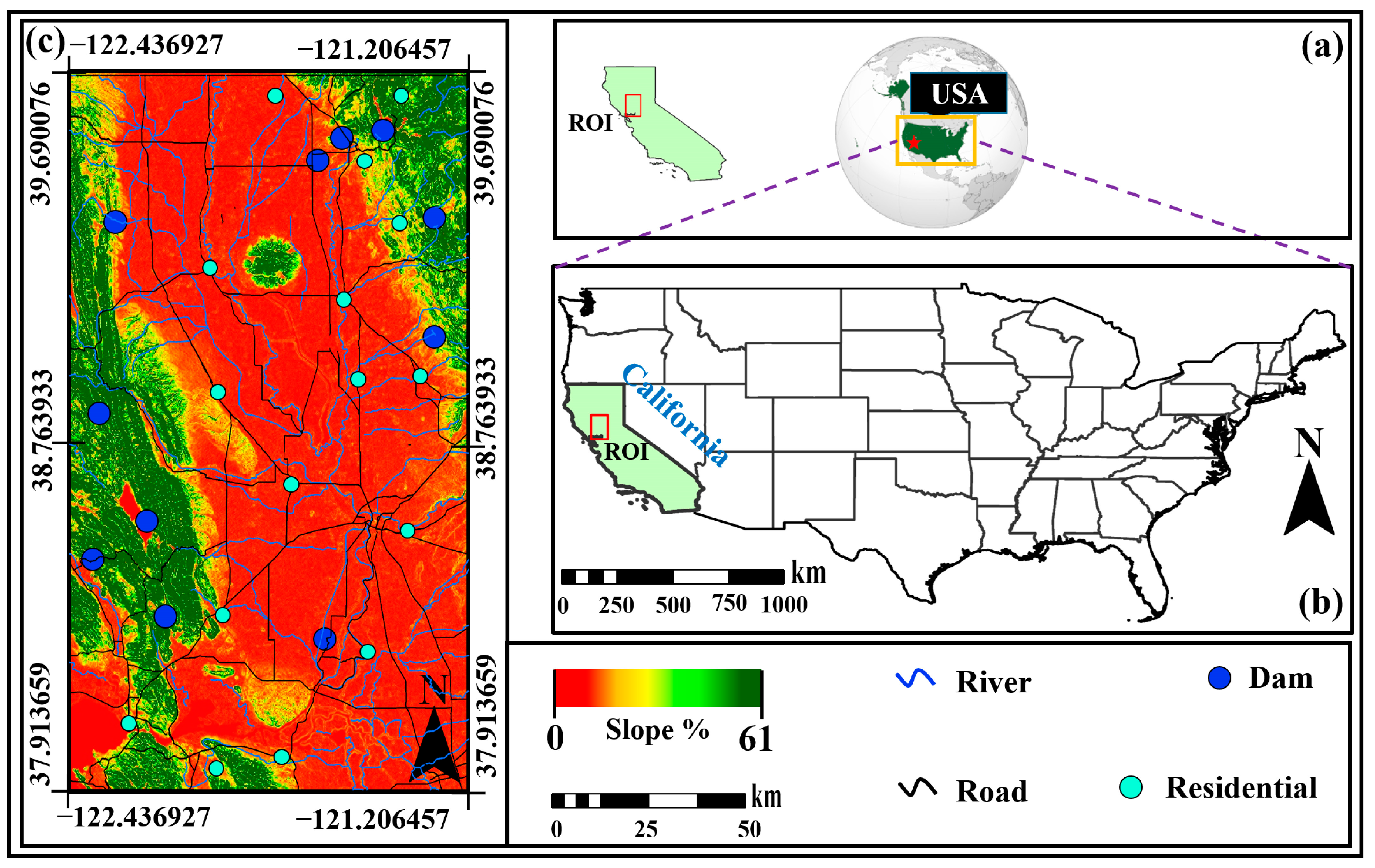
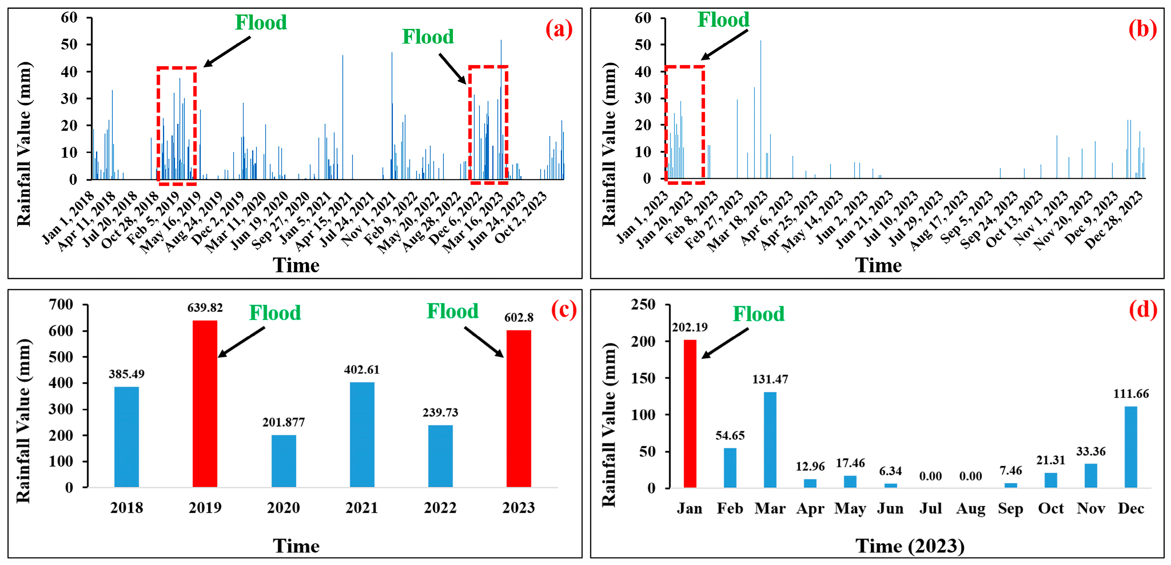
2.1. Study Areas

The city of Sacramento, located in the state of California, serves as the study area for this research, which experienced flooding in early 2023. California, one of the largest and most diverse states in the western U.S., holds significant economic, social, cultural, and natural importance. Additionally, California is known as a seismically active region and is prone to various natural hazards, including floods. In the past, flooding has had extensive impacts, particularly in coastal and mountainous areas of California. Moreover, as one of the most populous and vital states in the U.S., California’s floods can have profound effects on the population, economy, infrastructure, and environment. Impacts such as urban flooding, damage to agriculture and ecosystems, and disruptions in traffic and transportation are likely to occur as a result of flooding events. Geographically, California is known for its diverse landscapes, from the sunny southern coasts to the northern mountain ranges, resulting in varied climates and vegetation. Sacramento, the capital of California, is situated near the Sacramento River and its delta, which experienced severe flooding in early 2023 due to storms and excessive rainfall, exceeding the river’s capacity. The topography of the area ranges from elevations of −31 to 1356 m above sea level, with a maximum slope of 61%, significantly influencing runoff and flood formation. An overview of the study area is presented in Figure 1.

Figure 2 illustrates the precipitation levels in the study area. As depicted in chart (a) of Figure 2, the region has experienced a relatively stable and consistent daily rainfall pattern over the past six years. However, Figure 2c shows that the highest annual precipitation within this period occurred in 2019 (639.8 mm) and 2023 (602.8 mm). In 2019 and 2023, severe flooding struck the state of California, particularly in Sacramento, causing significant damage to urban infrastructure and agricultural lands. This study specifically examines the flood event of 2023. As shown in Figure 2, the average daily and annual precipitation in the study area over the past six years were 1.1 mm and 412.1 mm, respectively. Thus, rainfall in 2023 was approximately 190.7 mm higher than the regional average. Additionally, the average monthly precipitation in 2023, the year of the flood, was 49.9 mm. Precipitation in the first month of 2023, which led to the flood, was 202.2 mm—about 152.3 mm higher than the region’s monthly average. Rainfall exceeding 200 mm was recorded during the flood event. Specifically, precipitation in January was approximately 202.2 mm, while in February it was around 54.6 mm.

2.2. Data Collection and Data Pre-Processing

In this study, the proposed method was implemented using optical satellite images from Sentinel-2, Landsat-8, and Landsat-9. Additionally, Climate Hazards Group InfraRed Precipitation with Station data (CHIRPS) rainfall data were utilized to acquire prior knowledge of precipitation levels in the study area and to conduct subsequent analysis. Each dataset used in this research will be examined in greater detail in the following sections.

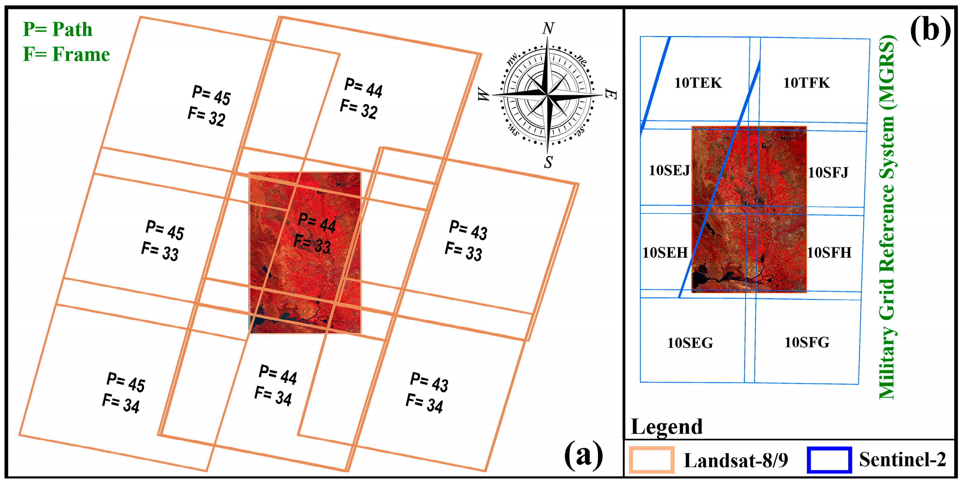
2.2.1. Sentinel-2 Satellite Imagery

The Sentinel-2 satellite imagery consists of two products, Sentinel-2A and Sentinel-2B, which were launched in 2015 and 2017, respectively. These satellites are equipped with 13 spectral bands spanning the visible, NIR, and Short-Wave Infrared (SWIR) regions, with spatial resolutions of 10 m, 20 m, and 60 m depending on the band. The revisiting time of Sentinel-2 images is 10 days if using data from just one satellite, and 5 days when both Sentinel-2A and 2B are combined, meaning that the same area can be re-imaged every 5 days. In the present study, Sentinel-2A/B have been utilized, specifically employing the bands with resolutions of 10 and 20 m. Figure 3b illustrates the footprint of Sentinel-2 images in the study area, providing coverage for the region under investigation. This combination of medium spatial and temporal resolution makes Sentinel-2 particularly suitable for monitoring dynamic environmental changes such as water bodies, vegetation health, and urban growth. The imagery data are publicly available from the GEE (https://developers.google.com/earth-engine/datasets/catalog/sentinel-2, accessed on 18 April 2024).

2.2.2. Landsat-8/9 Satellite Imagery

Landsat-8 and Landsat-9 are optical satellites launched on 11 February 2013, and 27 September 2021, respectively. They are widely used in various RS applications, including environmental monitoring, particularly for flood and surface water assessments. Therefore, this study also utilizes the sensors installed on the Landsat-8 and Landsat-9 satellites. These satellites encompass several spectral bands in the panchromatic, visible, and infrared ranges, with spatial resolutions ranging from 15 to 30 m, as well as two thermal bands with a spatial resolution of 100 m. Additionally, both satellites have a temporal resolution of 16 days; however, when utilizing both satellites, the temporal resolution improves to 8 days. Furthermore, Landsat-8 and Landsat-9 have radiometric resolutions of 12 and 14 bits, respectively. The footprints of the Landsat-8 and Landsat-9 images used in the study area are depicted in Figure 3a. The Landsat-8 imagery data are publicly available from the GEE (https://developers.google.com/earth-engine/datasets/catalog/landsat-8, accessed on 18 April 2024). The Landsat-9 imagery data are publicly available from the GEE (https://developers.google.com/earth-engine/datasets/catalog/landsat-9, accessed on 18 April 2024).

In the current research, images with cloud cover below 20% were employed for time-series flood identification. Subsequently, cloud-contaminated areas were masked using cloud removal bands from the images. The image collection corresponded to specific dates for flood identification, as illustrated in Figure 4.

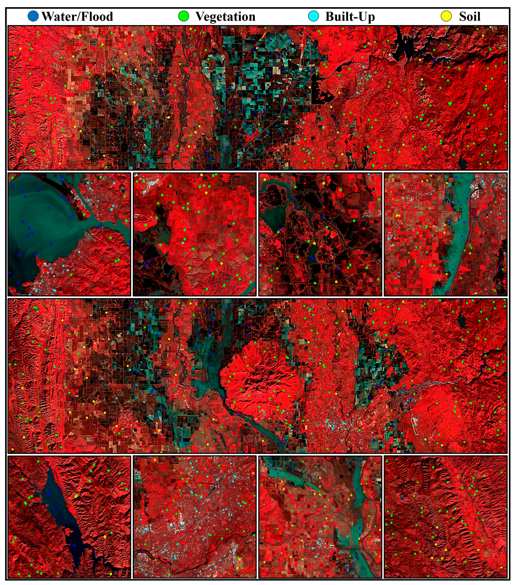
2.2.3. Test Samples Data

The test samples were collected to assess the accuracy of the proposed method in the study area through visual interpretation of Sentinel-2 imagery and High-Resolution (HR) images for the water/flood, urban, vegetation, and soil classes. Figure 5 illustrates the test samples gathered to evaluate the proposed method on Sentinel-2 and Landsat-8 images within the study area. As depicted in Figure 5, HR imagery available in Google Earth and corresponding-date Sentinel-2 images were used to assess the water/flood class. Moreover, test samples for other classes were also collected using High-Resolution imagery and Sentinel-2 images for classification accuracy assessment.

In Figure 5, images a–d correspond to water bodies captured in HR images, while images e–h represents urban areas within the study regions that were used for sampling. It is worth mentioning that the same sampling approach was employed for the evaluation of Landsat-9 images. In total, 800 samples were used to evaluate flood-affected areas, and 1700 samples were used for non-flooded areas. Therefore, the final flood map will be evaluated using the assessment samples for water/flood (target) and other samples (background).

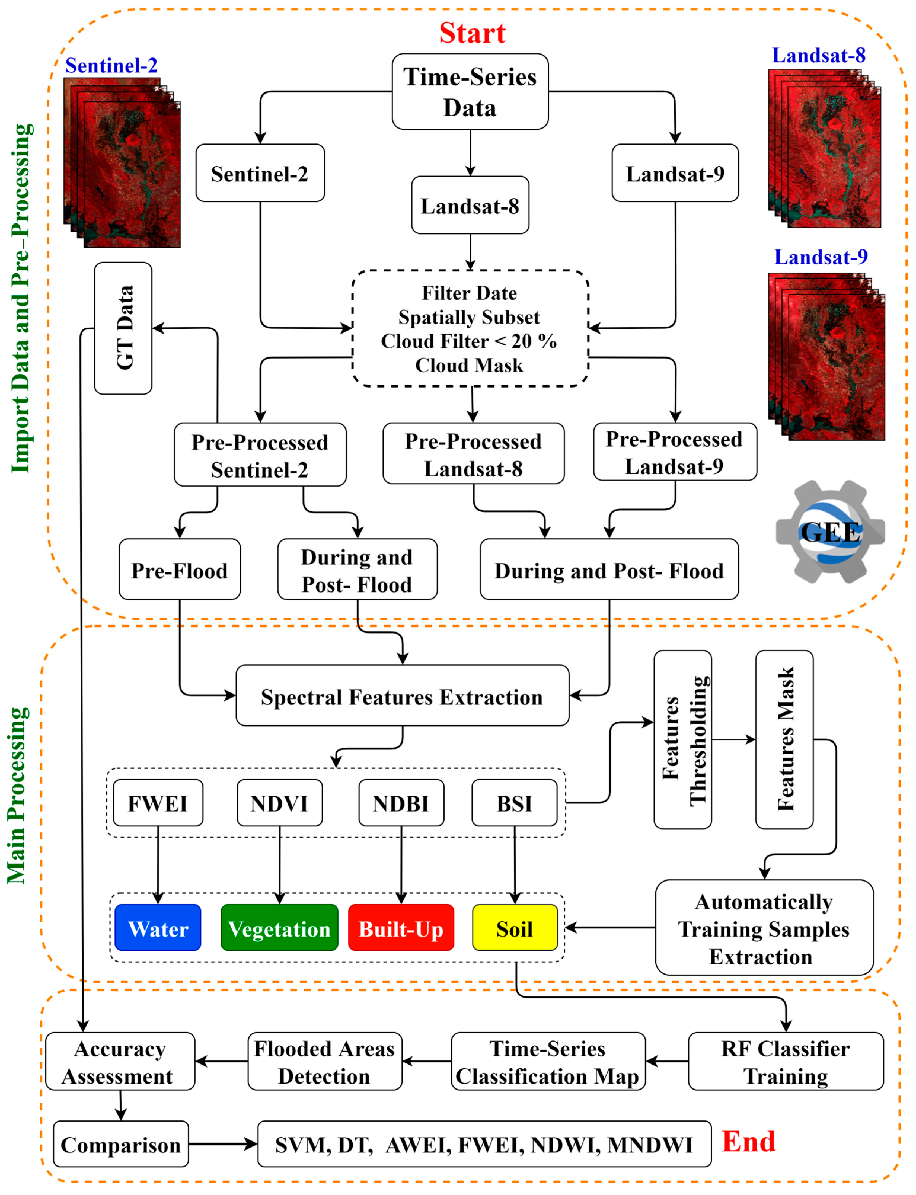
3. Methodology of the Research

This study utilizes multi-sensor satellite imagery from Sentinel-2, Landsat-8, and Landsat-9 to identify flood-affected areas by extracting relevant features and implementing an automated supervised classification. The implementation process of the proposed method is illustrated in the flowchart presented in Figure 6. The proposed method begins by importing time-series data from three satellite sources: Sentinel-2, Landsat-8, and Landsat-9. The imagery is filtered by temporal range and study area, ensuring cloud cover remains below 20%. A cloud mask is then applied using cloud filter bands to remove contaminated regions. After pre-processing, the images are categorized into pre-flood, during-flood, and post-flood periods. Spectral features are extracted using indices such as the FWEI, Normalized Difference Vegetation Index (NDVI), Normalized Difference Built-up Index (NDBI), and Bare Soil Index (BSI). These indices are used to automatically select training samples and classify key land cover types: water, vegetation, built-up areas, and soil. Feature thresholding is applied using the Otsu method to generate masks for each land cover class. Training samples are then randomly selected from the masks, and a Random Forest classifier is trained to produce a time-series classification map. The final flood map is created by subtracting the pre-flood classification from the during/post-flood classifications. The workflow concludes with an accuracy assessment and flood area detection. This automated approach, supported by GEE platform, facilitates NRT flood identification and monitoring through multi-sensor imagery.

3.1. Data Pre-Processing in GEE

GEE automatically performs orthorectification for Landsat-8, Landsat-9, and Sentinel-2 datasets, correcting atmospheric and geometric errors by default. As a result, all images are georeferenced, and no additional geometric or atmospheric correction is required. Radiometric corrections, aimed at reducing atmospheric and sensor errors, are also pre-applied in the GEE platform [52,53,54]. For datasets that are not pre-processed, GEE offers tools for efficient pre-processing, significantly reducing the steps typically needed in traditional RS methods, thus saving time [55]. The Landsat-8, Landsat-9, and Sentinel-2 datasets were filtered based on the study area boundary, time period, and a maximum cloud cover of 20%.

3.2. Extraction of Spectral Features

The FWEI, NDVI, NDBI, and BSI spectral indices were used to generate training samples for the water/flood, vegetation, built-up areas, and soil classes, respectively. Additionally, these indices, along with the primary satellite image bands, were utilized as spectral features for classification. Each index is discussed in detail below.

3.2.1. Flood/Water Extraction Index (FWEI)

The Flood/Waterbody Extraction Index (FWEI) is designed to enhance the detection of water bodies and flooded areas, by utilizing specific spectral bands from satellite imagery [5]. Equation (1) provides the methodology for computing this index.

$$FWEI={\displaystyle \frac{\left(\left(B+G+R\right)/3\right)-NIR}{\left(\left(B+G+R\right)/3\right)+NIR}}$$

(1)

The FWEI is calculated using the reflectance values from the blue, green, and red bands in relation to the NIR band. For Sentinel-2, the relevant bands for FWEI are Band 2 (Blue, 0.490 µm), Band 3 (Green, 0.560 µm), Band 4 (Red, 0.665 µm), and Band 8 (NIR, 0.842 µm). In Landsat-8 and Landsat-9, the corresponding bands are Band 2 (Blue, 0.450–0.515 µm), Band 3 (Green, 0.525–0.600 µm), Band 4 (Red, 0.640–0.670 µm), and Band 5 (NIR, 0.845–0.885 µm). The FWEI effectively differentiates water bodies from other land cover types by leveraging the spectral reflectance characteristics of water, which typically exhibit lower reflectance in the NIR band compared to visible bands [5]. Higher FWEI values indicate the presence of water, making it a useful tool for identifying both permanent and flooded areas.

3.2.2. Normalized Difference Vegetation Index (NDVI)

The NDVI is a widely used metric for extracting vegetation cover by comparing reflectance in the NIR and red bands [44]. NDVI is calculated as follows:

$$NDVI={\displaystyle \frac{NIR-R}{NIR+R}}$$

(2)

In Sentinel-2, the NIR band is Band 8 (0.842 µm), and the red band is Band 4 (0.665 µm). For Landsat-8 and Landsat-9, the NIR band is Band 5 (0.85–0.88 µm) and the red band is Band 4 (0.64–0.67 µm). Higher NDVI values reflect healthier vegetation, as plants strongly reflect NIR light and absorb red light. NDVI is highly effective for monitoring vegetation cover, biomass, and ecosystem health.

3.2.3. Normalized Difference Built-Up Index (NDBI)

The Normalized Difference Built-up Index (NDBI) is widely used to identify built-up areas in satellite imagery by leveraging the reflectance differences between the Short-Wave Infrared (SWIR) and near-infrared (NIR) bands [56]. NDBI is calculated as follows:

$$NDBI={\displaystyle \frac{SWIR-NIR}{SWIR+NIR}}$$

(3)

For Sentinel-2, the SWIR band is Band 11 (1.61 µm) and the NIR band is Band 8 (0.842 µm). In Landsat-8 and Landsat-9, the SWIR band corresponds to Band 6 (1.57–1.65 µm) and the NIR band to Band 5 (0.85–0.88 µm). Higher NDBI values indicate built-up areas, as these regions reflect more strongly in the SWIR than in the NIR, making it effective for distinguishing urban zones from other land cover types. Numerous studies have utilized this index for the extraction of urban areas and building footprints as a practical feature [57].

3.2.4. Bare Soil Index (BSI)

The Bare Soil Index (BSI) is a spectral index used to identify bare soil areas in satellite imagery by leveraging the unique reflectance characteristics of soil relative to other land cover types [58]. The index can be calculated using Equation (4).

$$BSI={\displaystyle \frac{\left(SWIR+Red\right)-\left(NIR+Blue\right)}{\left(SWIR+Red\right)+\left(NIR+Blue\right)}}$$

(4)

In Sentinel-2, the relevant bands are Band 11 (SWIR, 1.61 µm), Band 4 (Red, 0.665 µm), Band 8 (NIR, 0.842 µm), and Band 2 (Blue, 0.490 µm). For Landsat-8 and Landsat-9, the corresponding bands are Band 6 (SWIR, 1.57–1.65 µm), Band 4 (Red, 0.64–0.67 µm), Band 5 (NIR, 0.85–0.88 µm), and Band 2 (Blue, 0.45–0.51 µm). The BSI effectively distinguishes bare soil from other land cover types, as bare soil reflects more strongly in the SWIR and NIR bands while absorbing more in the blue and green bands. Higher BSI values indicate the presence of bare soil, making this index valuable for land cover classification, soil erosion assessment, and agricultural monitoring [58,59]. By applying the BSI to Sentinel-2, Landsat-8, and Landsat-9 imagery, researchers can improve their understanding of soil conditions and enhance land management practices.

3.3. Feature Thresholding for Land Cover Mask Generation

After calculating the spectral indices associated with water/flooded areas, vegetation, built-up regions, and bare soil, it is necessary to apply an optimal threshold to separate land cover classes from the background. Image classification can be conducted in two ways: manually and automatically. Manual threshold selection, particularly for large-scale and long-term studies, is complex and time-consuming, making it inefficient [5]. In 1979, Otsu introduced an unsupervised and automatic thresholding method for determining thresholds and binary image classification, which continues to be recognized as a valid approach in various remote sensing applications. This method maximizes the variance between two classes (background and foreground) based on the distribution of pixel values to derive an automatic threshold [60]. Therefore, in this study, the Otsu thresholding method was employed to differentiate the target (t) classes (water/flooded areas, vegetation, built-up regions, and bare soil) from the background (b). The Otsu threshold value is calculated as follows:

$${\sigma }^2(T_{index})=P_t(T)\times {\sigma }_t^2(T)+P_b(T)\times {\sigma }_b^2(T)$$

(5)

where σ is the weighted sum of variances of target and background pixels, Pt, σt, Pb, and σb are the probabilities and variances of the target and background classes separated by a threshold T, respectively. Therefore, the primary (Pr) and final (F) masks for the water/flood (W), vegetation (V), built-up (BU), and soil (S) classes can be calculated using Equations (6)–(9), respectively.

$$W_{\mathit{\text{F-Mask}}}=FWEI>T_{FWEI}$$

(6)

$$V_{\mathit{\text{Pr-Mask}}}=NDVI>T_{NDVI}$$

(7)

$$B{U}_{\mathit{\text{F-Mask}}}=NDBI>T_{NDBI}$$

(8)

$$S_{\mathit{\text{F-Mask}}}=BSI>T_{BSI}$$

(9)

Since the vegetation extracted by the Otsu method may classify bare soil as vegetation [5,61], the final bare soil map is generated by subtracting the primary vegetation mask (VPr-Mask). The final vegetation mask is then calculated using Equation (10).

$$V_{\mathit{\text{F-Mask}}}=V_{\mathit{\text{Pr-Mask}}}-S_{\mathit{\text{F-Mask}}}$$

(10)

Automated Generation of Training Samples

In this stage of the proposed method’s implementation, training samples are randomly selected from the generated masks for the water/flood, vegetation, built-up, and bare soil classes and are used to train the machine learning model. Since the maximum number of training samples is set to 10% of the total pixels for each class, the exact number of samples will vary in each image scene. In this study, the “randomPoints” function in GEE was employed to generate random sample points within the defined study region for training purposes. The “seed” parameter was used to control the random number generation process, ensuring reproducibility. By specifying a seed value, the same set of random points can be generated consistently across different runs, providing consistent results and eliminating variability caused by random sampling. For reproducibility, a seed value of 10 is used in the “randomPoints” function, ensuring that the same set of random points is consistently generated across multiple runs. This guarantees that during the optimization of the proposed method, the positions of the points remain fixed, preventing varying accuracies from being produced in different runs. This approach improves the consistency of results, as it ensures that the same set of representative training samples is used each time the model is trained. Furthermore, by minimizing variability in the selection of training samples, the method helps ensure more stable and accurate classification outcomes, reducing potential bias and enhancing the overall reliability of the model. These steps are crucial for achieving reproducible and reliable performance, especially in automated systems where random variation could otherwise lead to inconsistent accuracy.

3.4. Time-Series Classification of Flooded Areas

Following the generation of spectral indices, the creation of masks, and the automatic generation of training samples from various satellite images, time-series classification was conducted using the RF method. RF was selected for this study after being compared with DT and SVM, as it consistently achieved higher accuracy, demonstrated robustness to overfitting, and handled high-dimensional data more effectively. Unlike DT, RF mitigates overfitting by aggregating multiple trees, and compared to SVM, it requires less parameter tuning while providing insights into feature importance. Empirical results showed RF outperformed both DT and SVM in distinguishing flood-affected areas, making it the most reliable choice for this study. Further details are provided in the results section. The RF algorithm is a Machine Learning (ML) method widely used for classification tasks, including satellite image classification [18,39,40]. It builds multiple decision trees from random subsets of training data and features, which enhances robustness and reduces overfitting. This algorithm is particularly effective in handling high-dimensional datasets typical of image classification and managing complex interactions among numerous input features [62]. Additionally, RF offers valuable insights into feature importance, enabling researchers to identify variables that significantly influence classification outcomes. Its versatility and interpretability make RF a powerful tool for remote sensing applications and environmental monitoring. As a result, land cover was classified into four categories: water/flood, vegetation, built-up areas, and bare soil.

3.5. NRT Cumulative Flood Mapping

After generating the multi-class classification maps for the study area at different time points, the water/flood class will be extracted. The final flood map for each time will be produced by subtracting the permanent water extent from the post-flood water extent. By combining the results from each time step, a cumulative flood map will be generated as a time-series. The cumulative flood map, presented as a binary image, will indicate flood-affected areas (target) and non-flooded areas (background) throughout the flood period. Finally, the accuracy of the proposed method for extracting flood-affected areas will be evaluated using the test samples.

3.6. Results Evaluation

To assess the accuracy of the proposed method for extracting flood-affected areas, various accuracy assessment metrics derived from the error matrix were employed. These metrics include Overall Accuracy (OA), Kappa Coefficient (KC), Producer’s Accuracy (PA), and User’s Accuracy (UA). We categorized our pixels by comparing the extracted flood/water and non-flood/water pixels against test data. This resulted in four types of pixels: true positives (TPs), which signify the number of correctly identified water pixels; false negatives (FNs), representing the undetected water pixels; false positives (FPs), corresponding to the inaccurately classified water pixels; and true negatives (TNs), indicating the correctly identified non-water pixels [34,63]. The total number of pixels used for the accuracy assessment is denoted by T. Based on these pixel classifications, we calculated PA, UA, KC, and OA using Equations (11)–(14).

$$OA={\displaystyle \frac{TP+TN}{T}}$$

(11)

$$UA={\displaystyle \frac{TP}{TP+FP}}$$

(12)

$$PA={\displaystyle \frac{TP}{TP+FN}}$$

(13)

$$K={\displaystyle \frac{OA-Pe}{1-Pe}}\Rightarrow Pe={\displaystyle \sum _{i=1}^n\frac{(T{P}_i+F{P}_i)(T{P}_i+F{N}_i)}{N^2}}$$

(14)

4. Results and Discussion

In this section, the results obtained from the proposed method will be presented, covering various aspects of the current research. This includes the results of training sample generation, the outcomes of time-series classification mapping, the identification of flood-affected areas, the cumulative identification of flood-affected regions, and the qualitative and quantitative accuracy assessment. Each aspect will be discussed concurrently to provide a comprehensive understanding of the findings.

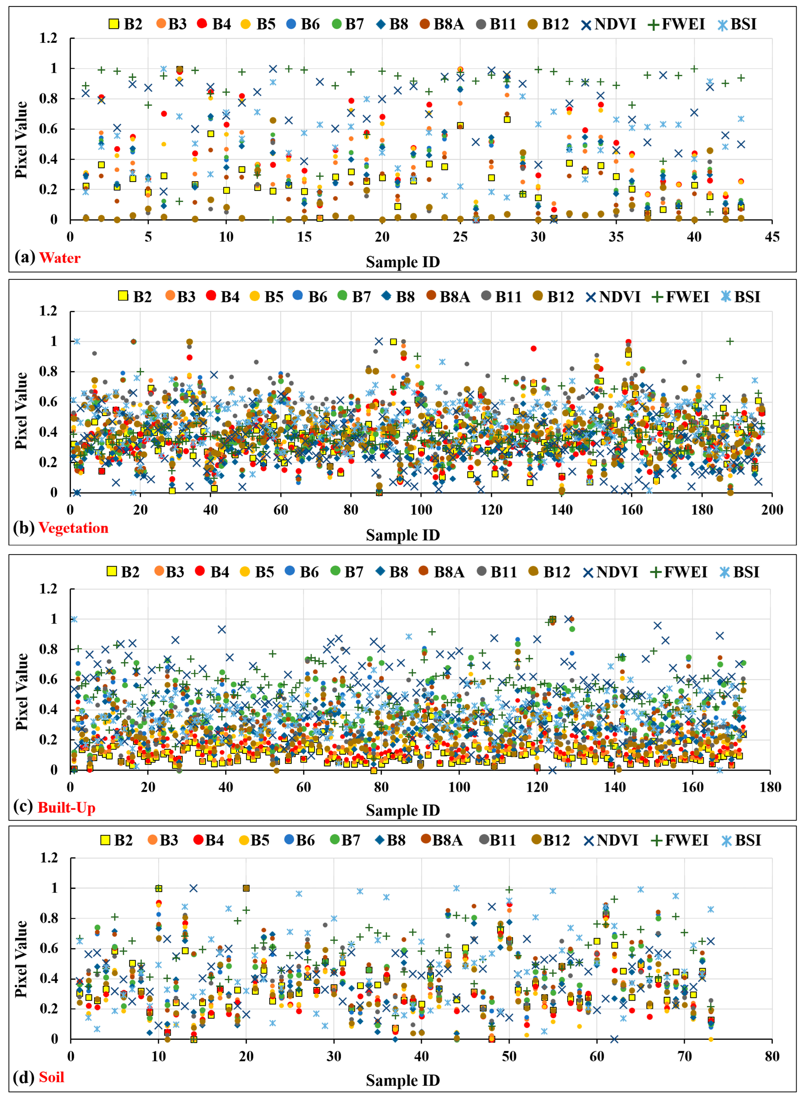
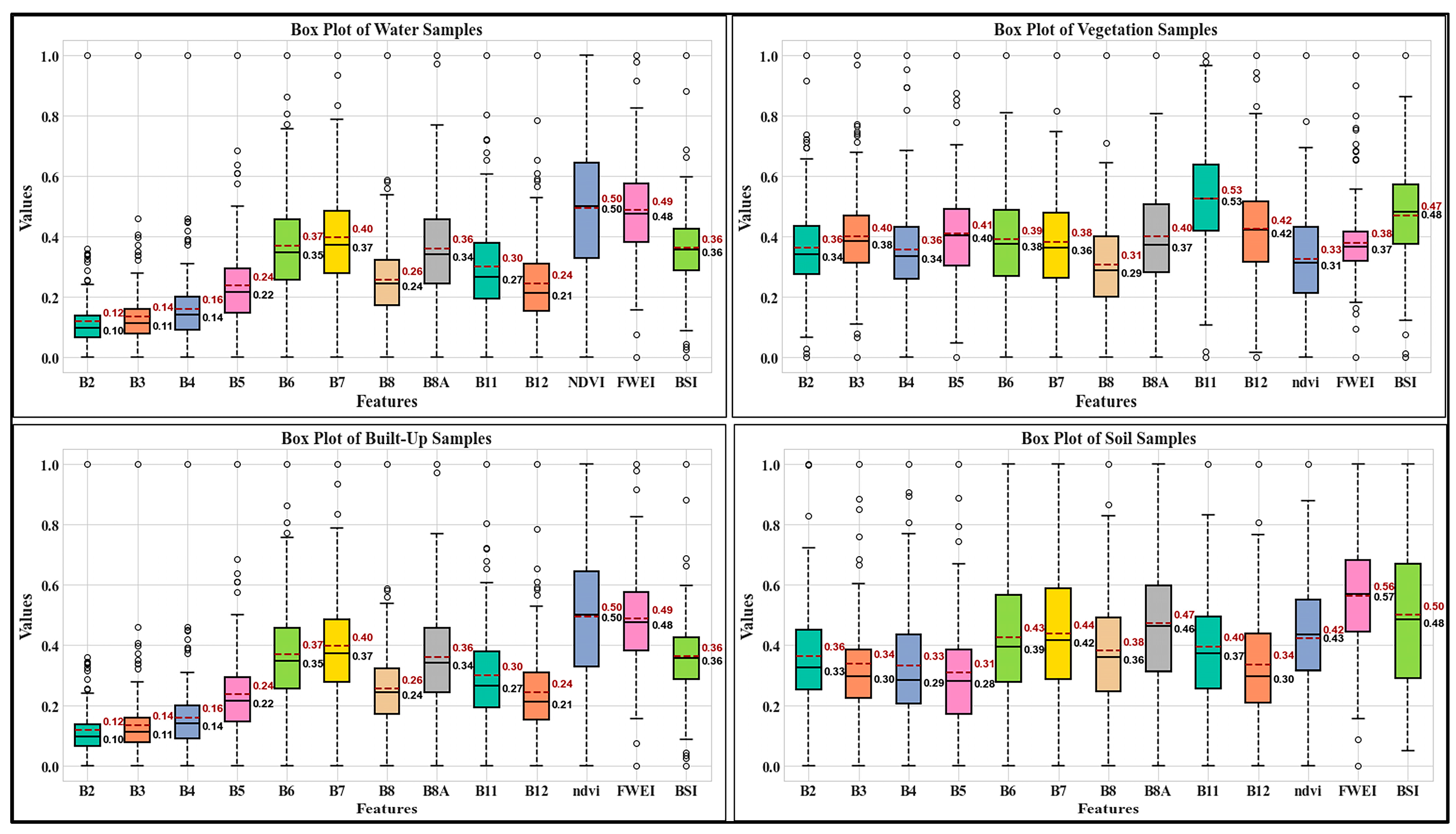
4.1. Result of Training Samples Generation

The training samples extracted by the proposed method for a portion of the study areas are presented in Figure 7. As shown in this figure, the training samples exhibit a uniform distribution across the region.

In Figure 8, the spectral behavior of automatically extracted training samples across different bands and spectral indices is depicted, offering insights into the variability and distribution of pixel values for four land cover types: (a) water, (b) vegetation, (c) built-up areas, and (d) soil. Each plot represents a range of spectral bands (B2, B3, B4, B5, B6, B7, B8, B11, and B12) and commonly used spectral indices (NDVI, FWEI, and BSI), plotted against the sample ID.

The plots reveal distinct spectral signatures, with water exhibiting lower reflectance across most bands, especially in the visible and NIR regions, while vegetation shows higher reflectance in the NIR band (B8). Built-up areas demonstrate greater variation across bands, reflecting their heterogeneous nature, and soil samples display a more balanced reflectance, with notable responses in the Short-Wave Infrared bands (B11 and B12). This detailed analysis aids in understanding the spectral variability between different classes, which is critical for the classification and monitoring of land cover changes in remote sensing applications.

The plots reveal distinct spectral signatures, with water exhibiting lower reflectance across most bands, especially in the visible and NIR regions, and vegetation showing higher reflectance in the NIR band (B8). Built-up areas demonstrate greater variation across bands, reflecting their heterogeneous nature, and soil samples display a more balanced reflectance, with notable responses in the Shor-Wave Infrared bands (B11 and B12). This detailed analysis aids in understanding the spectral variability between different classes, which is critical for the classification and monitoring of land cover changes in remote sensing applications.

The box plots in Figure 9 illustrate the spectral characteristics of four land cover classes—water, vegetation, built-up areas, and soil—across various Sentinel-2 bands and indices (B2, B3, B4, B5, B6, B7, B8, B11, B12, NDVI, FWEI, and BSI). Each plot reveals distinct reflectance patterns for the different classes. Water samples show lower reflectance in the visible and infrared bands, particularly in B8 and B11, while vegetation exhibits higher values in the NIR region, which is characteristic of healthy vegetation. Built-up areas display greater variability across all bands, particularly in B11 and B12, reflecting the heterogeneity of urban materials. Soil samples have relatively balanced reflectance across bands, with notable variability in the SWIR region (B11, B12). Figure 7, Figure 8 and Figure 9 illustrate that the training samples extracted using the proposed method exhibit an optimal distribution across the spectral ranges of the bands and indices, contributing to higher accuracy in model training. Furthermore, the box plot in Figure 9 demonstrates the effectiveness of using spectral indices in the machine learning process. Consequently, the automatically generated training samples are highly valid for land cover classification, particularly for water bodies.

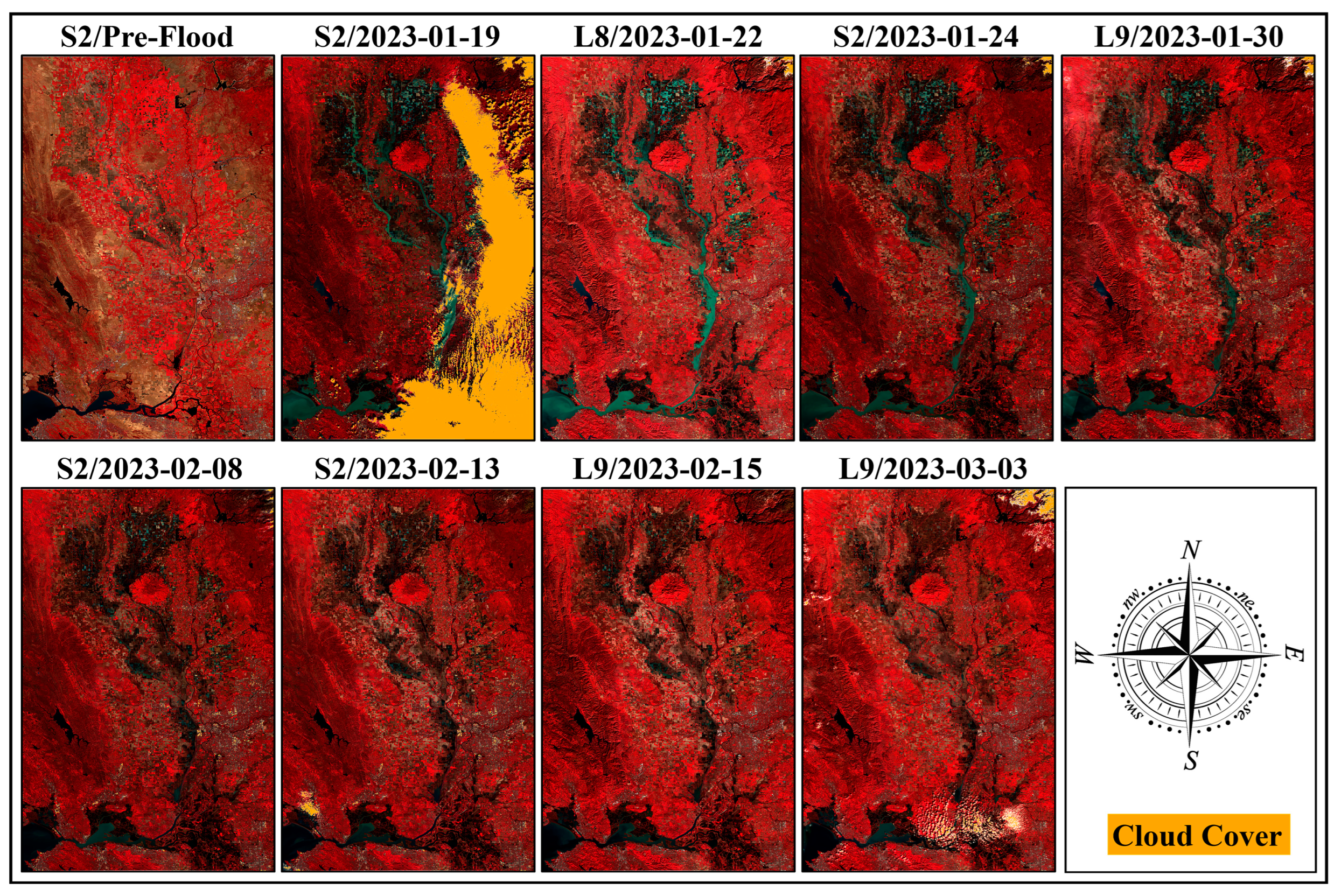
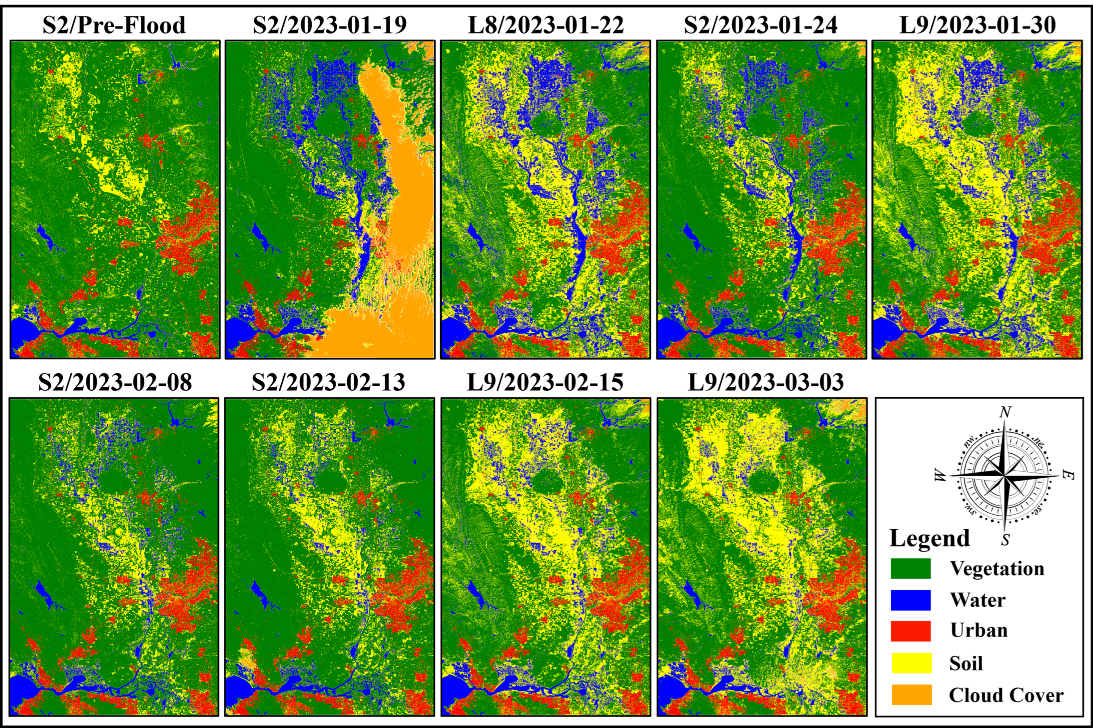
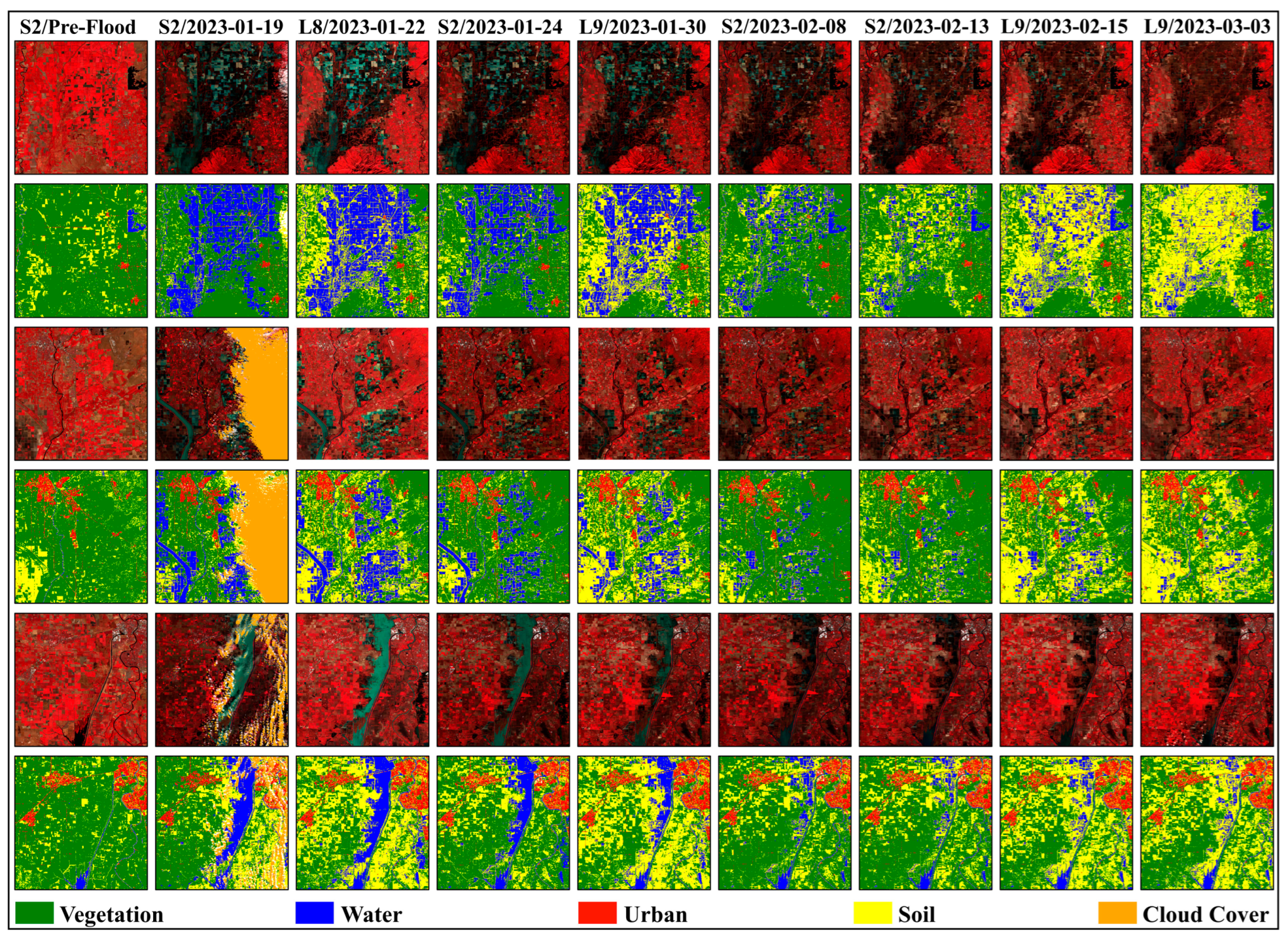
4.2. Result of Time-Series Classification Map

The results of the proposed method using RF classification, based on multi-sensor and multi-temporal imagery across four different classes, are presented in Figure 10. As shown, four maps correspond to Sentinel-2 images, one to Landsat-8, and three to Landsat-9, covering the flood period in the study area. It is important to note that the cloud cover class was derived using cloud cover bands and added to the classification maps for improved visualization. As illustrated in Figure 10, despite the extensive cloud cover in the western part of the study area in the Sentinel-2 image from 19 January 2023, which leaves no data for certain classes, the proposed method, utilizing multi-sensor images with a 3-day temporal gap, successfully identified water bodies in that region. Visually, the method effectively delineated four classes: water/flood, vegetation, built-up areas, and soil.

The results indicate an expansion of the water/flood extent compared to the pre-flood image. Moreover, due to heavy rainfall and flooding, which destroyed vegetation, the soil class area increased compared to the pre-flood image. Therefore, the proposed method demonstrates reliable accuracy in capturing land use changes, with the accuracy of each class evaluated in the accuracy assessment section. Figure 11 presents portions of the study area with different land covers as extracted by the proposed method.

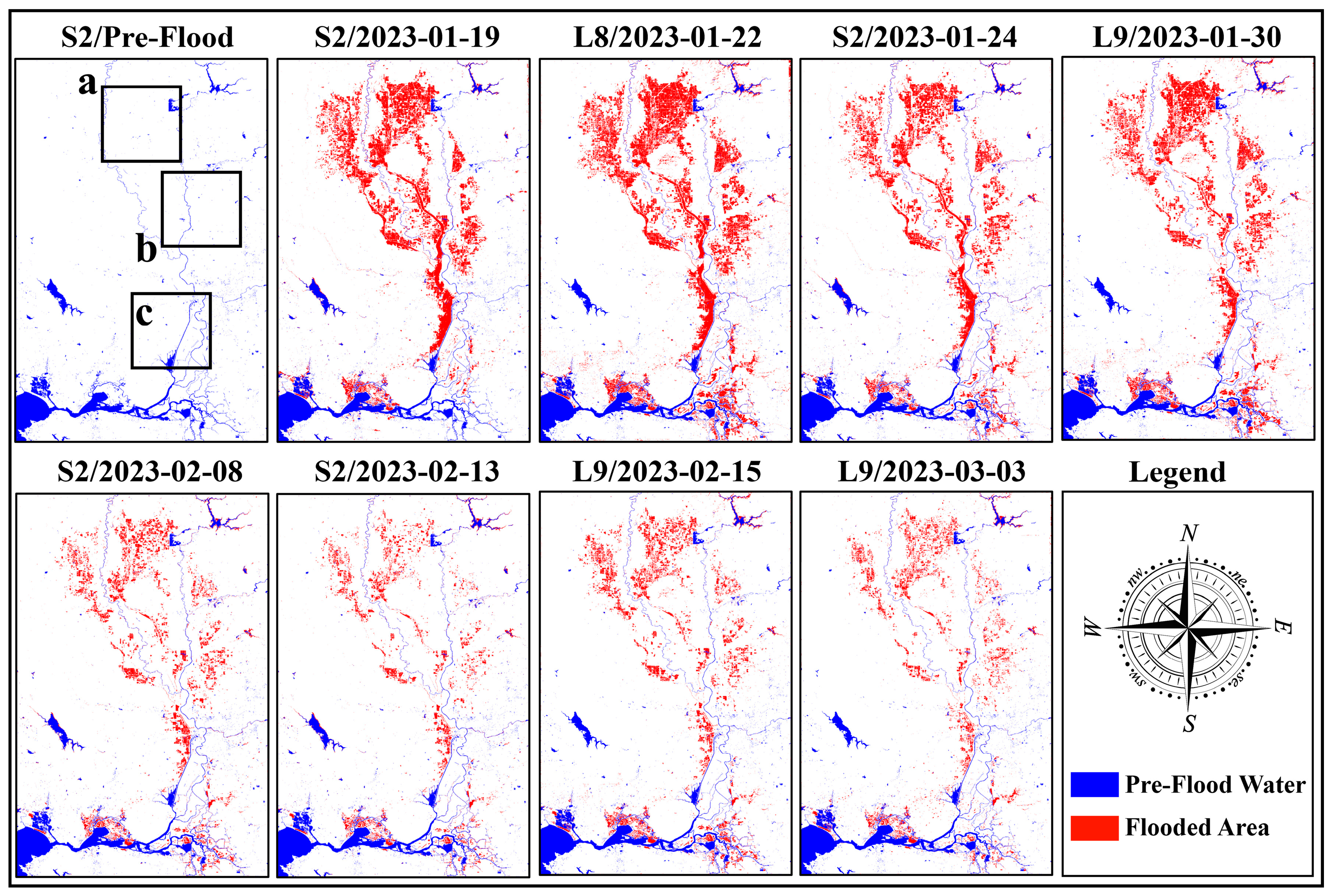
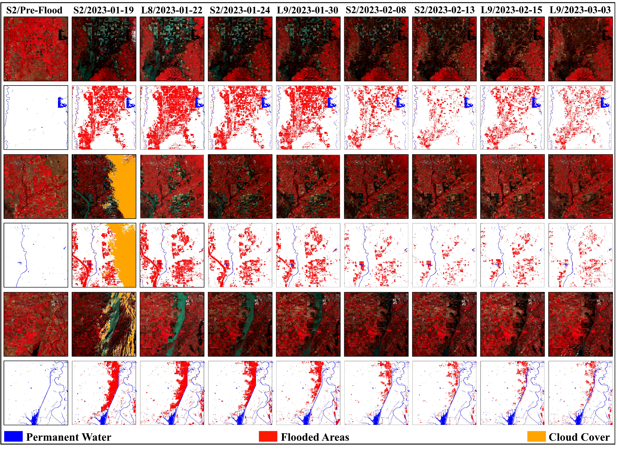
4.3. Result of NRT Flood Mapping

The results of flood-affected area identification, presented as a time-series using multi-sensor imagery for the study area, are shown in Figure 12. As illustrated, the changes in flood extents over time have been detected using data from various sensors. Despite the temporal resolution of Sentinel-2 imagery being 5 days and that of Landsat-8 and Landsat-9 being 16 days, the proposed method enables flood monitoring in the first three time points with a temporal resolution of 2–3 days by integrating imagery from multiple satellites. Therefore, using this approach, near real-time flood monitoring in a time-series format has been achieved. Based on the temporal resolution of each satellite and the percentage of cloud cover in the region, a temporal gap can occur in flood monitoring. This gap may result in the inability to detect flood-affected areas during specific time intervals. Therefore, the availability of more images from the region, combined with lower cloud cover, enables flood monitoring at much shorter intervals, potentially as close as 1 to 2 days. The spatial resolution of each flood map corresponds to the imagery used. In other words, the spatial resolution of the generated flood maps is 10 m for Sentinel-2 and 30 m for Landsat-8 and Landsat-9.

Portions of the flooded areas (a, b, and c) are presented in Figure 12 for improved visual interpretation, and the flood progression is illustrated in Figure 13. As demonstrated by three different regions in Figure 13, the proposed method effectively models the flooding process using multi-sensor, multi-temporal images, providing a time-series analysis with high spatial resolution. Consequently, the proposed method allows for near real-time assessment of damage to various land covers through time-series data. Thus, it can be concluded that, in the absence of heavy cloud cover, optical images from different sensors can also be utilized for flood mapping and detection.

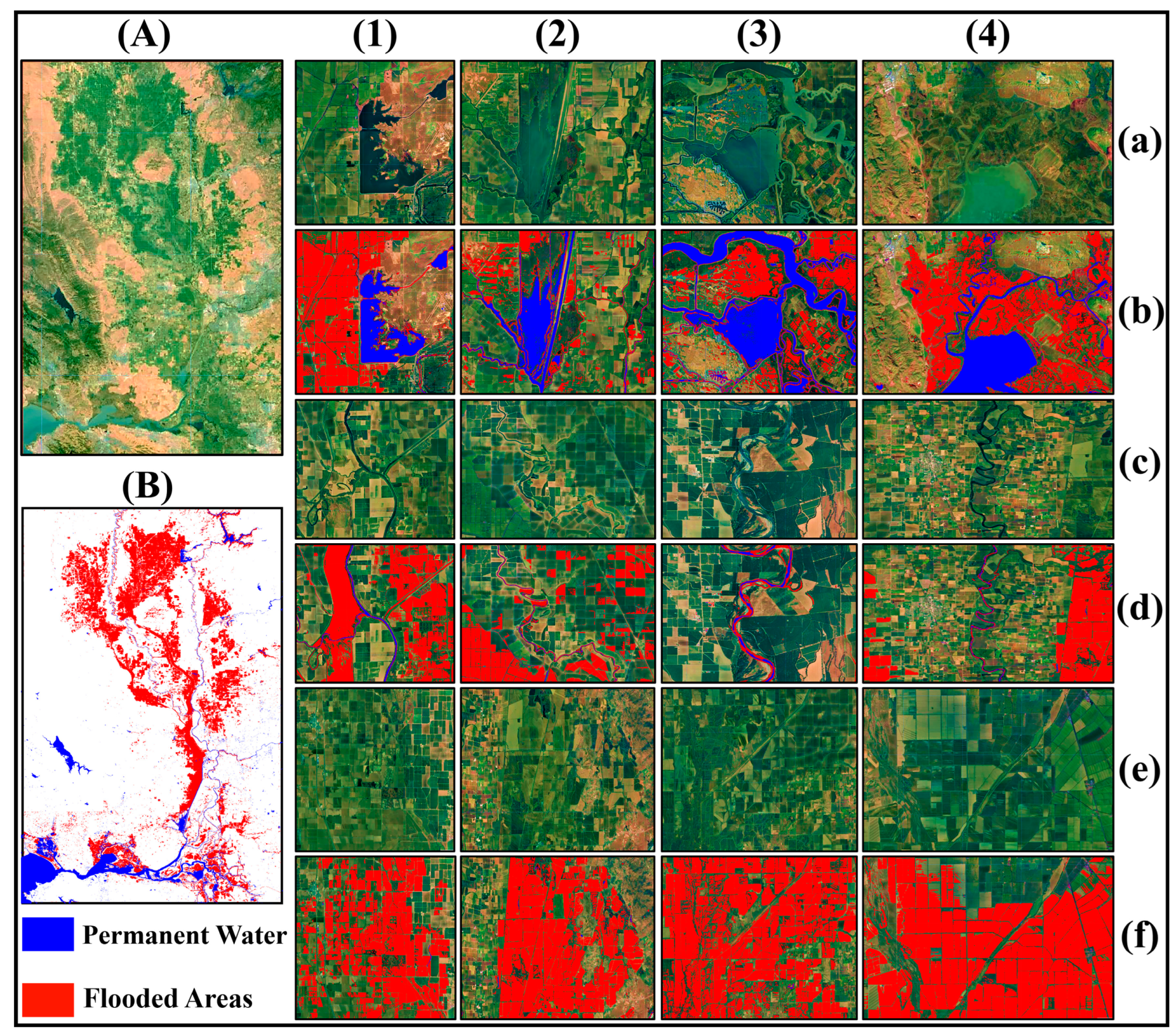
4.4. Extraction of Water and Flooded Areas Using the Proposed Method

To evaluate the potential of the proposed method for flood detection across various land uses, flood identification was conducted along riverbanks, vegetated areas, and regions containing reservoirs and lakes, as shown in Figure 14. This figure presents four areas containing water bodies and lakes (Figure 14a), four riverine areas (Figure 14c), and four vegetated regions (Figure 14d), all analyzed using High-Resolution imagery from Google Earth (Figure 14A) alongside the flood detection results (Figure 14B). As depicted in Figure 14, the proposed method demonstrates strong potential for extracting water and flooded areas in rivers (Figure 14d), reservoirs (Figure 14b), and vegetated regions (Figure 14f). Thus, the method is highly suitable for identifying vegetation damaged by floods, aligning with the findings of [5]. Additionally, the proposed approach effectively extracts flood-affected areas around rivers, reservoirs, and coastal zones, also consistent with previous studies [16,17,43]. Therefore, the results indicate the effectiveness of the proposed method for NRT flood monitoring.

4.5. Accuracy Assessment of the Results

In this section, the accuracy of the land cover classification maps produced by the proposed method will be evaluated. Additionally, the accuracy of identifying and extracting flood-affected areas will be assessed. Furthermore, a quantitative comparison between the proposed method and other existing techniques and indices for flood detection will be conducted.

4.5.1. Land Cover Classification Accuracy Assessment

The accuracy assessment of the proposed land cover classification method, as presented in

Table 1. Accuracy assessment of the proposed method (with RF) for land cover classification.

Image Scene	Class	UA	PA	OA	KC
S2-2023/01/24	Flood/Water	91.23	92.42	89.96	0.89
	Vegetation	90.14	90.17
	Built-Up	68.64	69.12
	Soil	79.34	80.05
L8-2023/01/22	Flood/Water	90.58	90.87	87.68	0.86
	Vegetation	89.93	88.99
	Built-Up	66.49	67.06
	Soil	79.64	79.85
L9-2023/02/15	Flood/Water	90.05	90.59	88.84	0.88
	Vegetation	90.43	90.62
	Built-Up	69.26	70.09
	Soil	79.81	80.28

, shows that the flood/water class consistently achieves the highest accuracy across all three sensors (Sentinel-2, Landsat-8, and Landsat-9). Sentinel-2 imagery yields an OA of 89.96% with a KC of 0.89, indicating a strong alignment with test data. The flood/water class demonstrates UA and PA exceeding 91%, while the vegetation class also performs well, with accuracies around 90%. However, the built-up class exhibits the lowest accuracy, with both UA and PA below 70%, likely due to the difficulty in distinguishing urban areas from other land cover types. Also, Landsat-8 and Landsat-9 show slightly lower overall accuracies, at 87.68% and 88.84%, with a corresponding KC of 0.86 and 0.88. Despite these differences, all sensors exhibit strong classification performance, particularly for the flood/water and vegetation classes. The soil class maintains moderate accuracy across the sensors, with accuracies close to 80%. Overall, the proposed method proves effective for land cover classification, with Sentinel-2 imagery outperforming the others due to its superior spatial resolution. The lower accuracy in the built-up class suggests room for improvement, but the method’s consistency across multiple sensors underscores its potential for reliable flood mapping and land cover classification.

4.5.2. Flood Detection Accuracy Assessment

In addition to assessing the accuracy of the land cover classification results, the flood-affected areas were also evaluated quantitatively. To evaluate the accuracy of the proposed method for identifying flood zones, the water/flood class from each image was subtracted from the corresponding pre-flood image, and the remaining areas were considered as flooded regions. The other classes (vegetation, built-up areas, and soil) were classified as non-flooded areas. The accuracy assessment results for the proposed method in extracting flood-affected areas are presented in

Table 2. Accuracy assessment of the proposed method of flood detection.

Image Scene	Class	UA	PA	OA	KC
S2-2023/01/24	Flooded	92.24	92.58	92.03	0.91
	Non-Flooded	89.39	90.61
L8-2023/01/22	Flooded	90.19	90.49	89.14	0.88
	Non-Flooded	88.66	89.63
L9-2023/02/15	Flooded	89.97	90.09	90.54	0.89
	Non-Flooded	88.81	89.42
Average	Flooded	90.8	90.05	90.57	0.89
	Non-Flooded	88.95	89.89

.

The accuracy assessment for the proposed flood detection method, detailed in Table 2, reveals that the highest accuracy of detection for flooded areas is obtained using Sentinel-2 imagery from 24 January 2023. This dataset demonstrates a UA of 92.24%, a PA of 92.58%, and an OA of 92.03%. A KC of 0.91 indicates a strong agreement with test samples data. In comparison, although the OA of Landsat-8 and Landsat-9 imagery is slightly lower, both sensors exhibit robust performance; Landsat-8 imagery from 22 January 2023, achieves an OA of 89.14% with a KC of 0.88, while Landsat-9 imagery from 15 February 2023 achieves an OA of 90.54% and a KC of 0.89. Notably, the flooded class shows high UA and PA, exceeding 90% in both cases. Furthermore, non-flooded areas are effectively detected, with user and producer accuracies averaging approximately 88.95% and 89.89%, respectively, across all sensors, underscoring the robustness of the method for detecting both flooded and non-flooded areas. Therefore, the proposed method consistently achieves high accuracy in flood detection across all satellite images, with Sentinel-2 slightly outperforming due to its higher spatial resolution. This analysis highlights the effectiveness and reliability of the method for NRT flood monitoring, with the highest accuracy values in Table 2, clearly illustrating the superior performance of Sentinel-2 imagery.

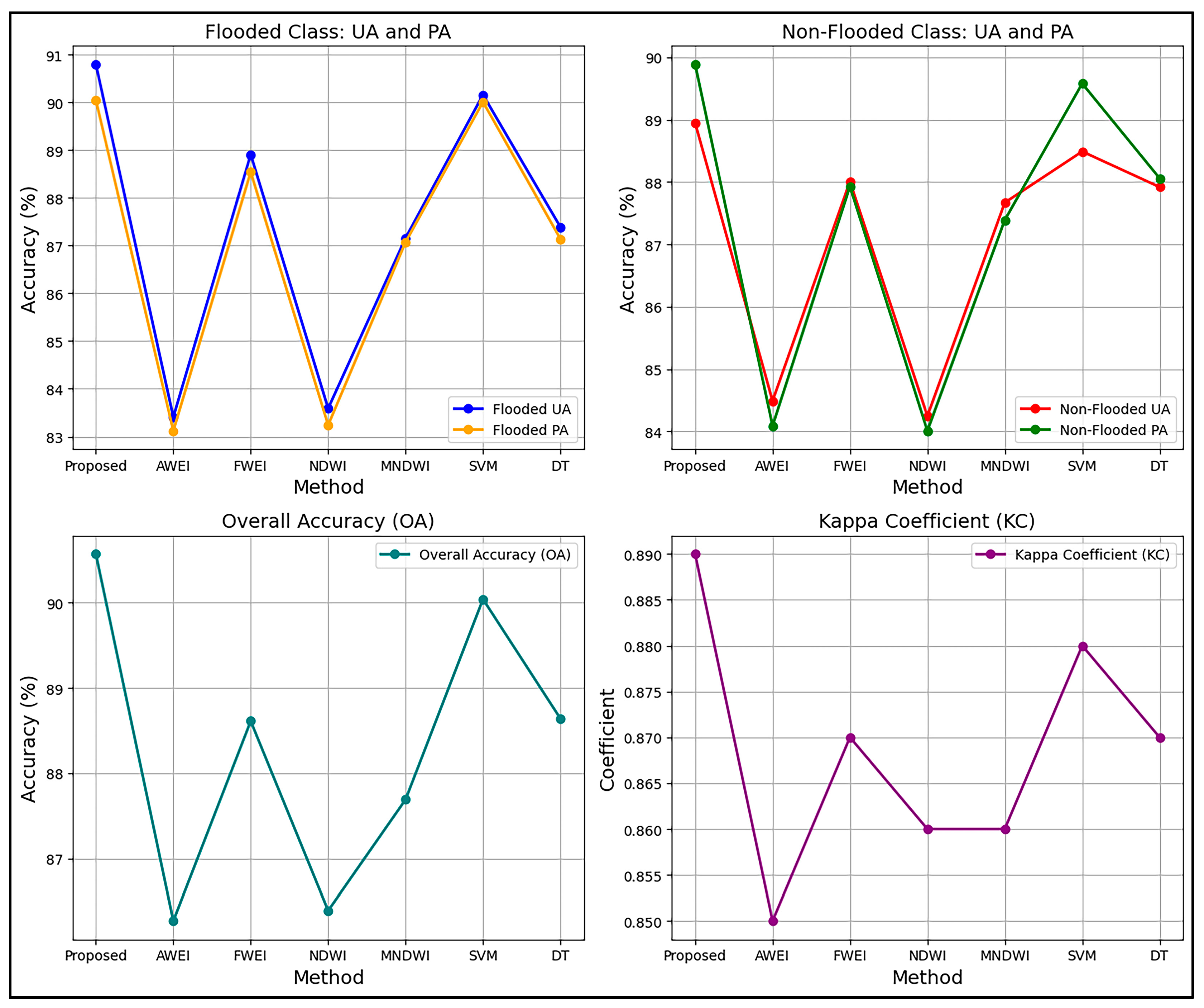
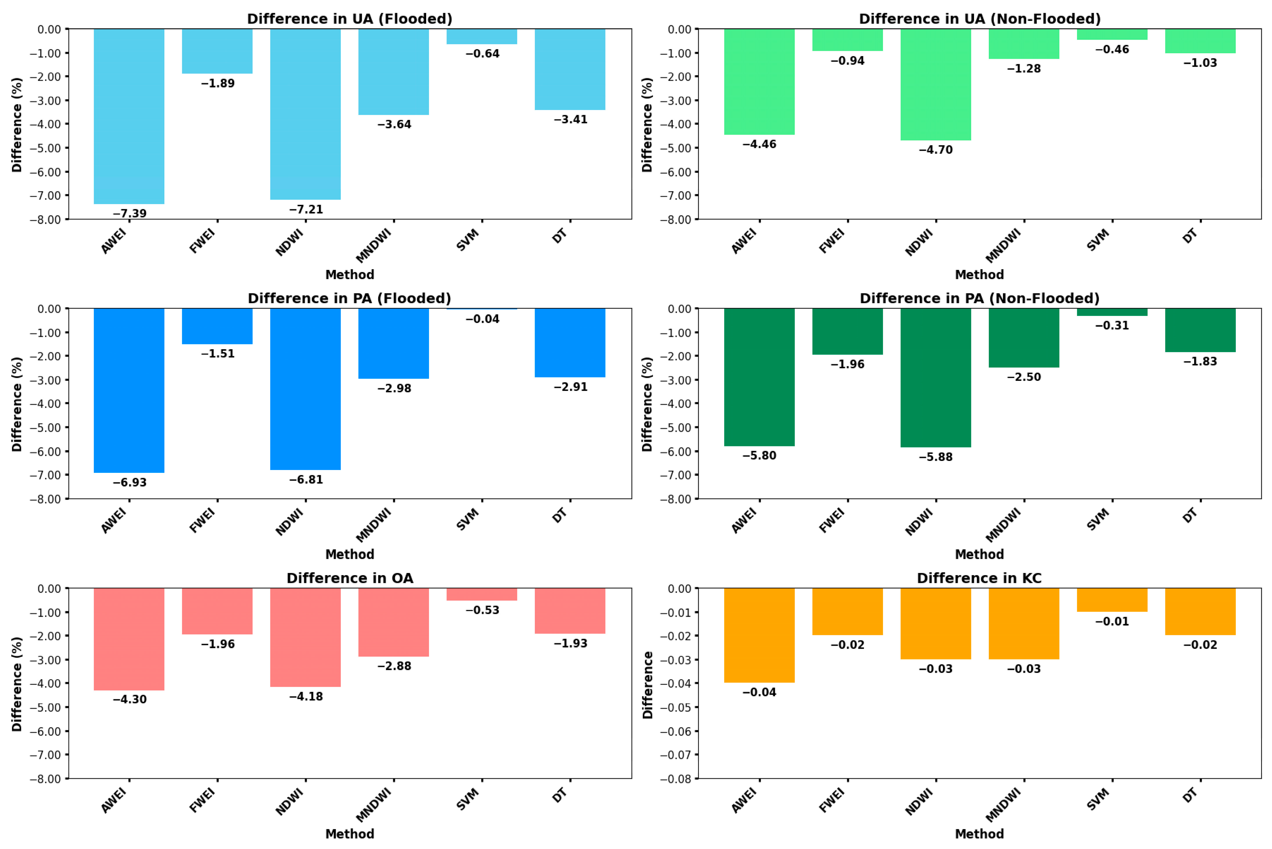
4.5.3. Comparing the Accuracy of the Proposed Method and Other Methods

Table 3. Performance comparison of the proposed method and other approaches.

Method	Class	UA	PA	OA	KC
Proposed (Average)	Flooded	90.8	90.05	90.57	0.89
	Non-Flooded	88.95	89.89
AWEI	Flooded	83.41	83.12	86.27	0.85
	Non-Flooded	84.49	84.09
FWEI	Flooded	88.91	88.54	88.61	0.87
	Non-Flooded	88.01	87.93
NDWI	Flooded	83.59	83.24	86.39	0.86
	Non-Flooded	84.25	84.01
MNDWI	Flooded	87.16	87.07	87.69	0.86
	Non-Flooded	87.67	87.39
SVM	Flooded	90.16	90.01	90.04	0.88
	Non-Flooded	88.49	89.58
DT	Flooded	87.39	87.14	88.64	0.87
	Non-Flooded	87.92	88.06

presents a comparative analysis of the proposed flood detection method against several alternative approaches, including spectral indices (AWEI, FWEI, NDWI, and MNDWI) and popular ML methods (SVM and DT), using key performance metrics such as UA, PA, OA, and the KC. Notably, the proposed method achieves the highest performance across all metrics, particularly excelling in the detection of flooded areas with a UA of 90.8% and a PA of 90.05%. This strong performance is also reflected in the non-flooded class, where the suggested method records a UA of 88.95% and a PA of 89.89%. Moreover, the proposed method attains the highest OA at 90.57% and a KC of 0.89, indicating excellent agreement between predicted and actual classifications, further supporting its overall robustness.

In contrast, alternative methods such as AWEI and FWEI exhibit lower performance, with AWEI showing the weakest results for the flooded class (PA of 83.12%) and moderate accuracy overall. While FWEI improves slightly with UA and PA around 88% for flooded areas, it still falls short of the proposed method’s reliability. Similarly, NDWI has lower UA and PA values for flooded areas, indicating less effectiveness in accurately detecting these regions. MNDWI improves upon this slightly, with UA and PA values exceeding 87%, yet it remains behind the proposed approach in overall performance.

Among the alternative methods, SVM stands out as the closest competitor to the proposed method. SVM achieves nearly identical performance for flooded areas (UA: 90.16%, PA: 90.01%) and records a slightly lower OA (90.04%) and KC (0.88), suggesting it is a strong alternative but still marginally less effective. Finally, the DT method, while showing solid performance in both classes with UA and PA around 87–88%, also trails behind the proposed method in OA (88.64%) and KC (0.87).

Therefore, the proposed method outperforms all aforementioned approaches, particularly in flood detection, where it demonstrates superior accuracy and consistency. While SVM serves as a competitive option, the performance of AWEI, FWEI, NDWI, and MNDWI is marked by substantial decreases in accuracy, making them less dependable for accurate flood detection. Therefore, the proposed approach offers greater reliability for NRT flood mapping. The chart in Figure 15 illustrates the accuracy assessment metrics for the proposed method (with RF) and other flood delineation methods. Also, the results of the comparison between the proposed method and other methods are presented in the charts of Figure 16.

4.6. Impact of Training Sample Size on Classification Accuracy Metrics

Figure 17 examines the impact of training sample size (ranging from 7% to 13%) on classification accuracy metrics, including UA, PA, OA, and KC. This analysis was conducted using satellite images from Sentinel-2, Landsat-8, and Landsat-9 to assess the sensitivity of classification performance to variations in training data proportions. The findings indicate that changes in training sample size have minimal effect on accuracy metrics. For instance, Sentinel-2 consistently achieves an overall accuracy above 92% (average 92.03%), while Landsat-8 and Landsat-9 yield average values of approximately 89.15% and 89.01%, respectively. Similarly, the UA for Sentinel-2 ranges from 92.01% to 92.25%, whereas Landsat-8 and Landsat-9 exhibit ranges of 89.55–89.87% and 90.12–90.20%, respectively. This stability highlights the robustness of classification results against variations in training sample size. A one-way ANOVA analysis revealed no statistically significant differences in accuracy metrics across different training sample sizes (p-value > 0.05). However, significant differences were observed in the classification maps produced by the three satellites. These differences appear to be driven by spatial resolution rather than sample size. Sentinel-2, with its higher spatial resolution of 10 m, consistently outperformed Landsat-8 and Landsat-9, which have a 30 m resolution, across all metrics. The low standard deviation values for all metrics (less than 0.1%) underscore the consistency and reliability of the results. Overall, the findings emphasize the advantage of higher spatial resolution imagery, such as Sentinel-2, in improving classification accuracy, irrespective of the proportion of training samples used.

4.7. Advantages and Limitations of the Proposed Method

The present study aimed to identify flood-affected areas in NRT using multi-source satellite imagery. A critical step in supervised classification is the extensive need for training samples, which poses a significant challenge in time-series analysis. However, the proposed approach in this study overcomes this challenge by automatically generating training samples, which is a key advantage of this research. Another benefit of this approach is its implementation in the GEE platform, reducing computational time and enabling the execution of essential pre-processing steps for time-series analysis. Additionally, it enhances the level of automation in generating training samples.

A further advantage of the proposed approach is the use of multi-source optical imagery, allowing for NRT flood mapping. Nevertheless, this study has some limitations. One notable drawback is the method’s weakness in detecting flood-affected areas when shadows are present. Moreover, since the sampling process relies on thresholding to create feature masks (flooded/water areas, vegetation, built-up areas, and soil), some samples may be inaccurately classified. Despite these limitations, the proposed approach demonstrates high accuracy in delineating water bodies, though it is less suitable for urban mapping. Overall, based on the comparisons conducted in this study, the proposed method shows significant potential for time-series flood mapping using multi-sensor satellite imagery, outperforming other methods.

5. Conclusions

Accurate identification and mapping of flood-affected areas are crucial for relief efforts, urban management, insurance services, and reconstruction. Remote sensing with satellite imagery offers a key solution for this task. Various methods for flood detection exist, depending on regional weather conditions, image type, and land cover. Spectral index thresholding and supervised classification are common approaches, but challenges arise with threshold dependency and the need for training samples in supervised machine learning, especially for multi-temporal, multi-sensor flood mapping. To address these challenges, this study proposes an automated framework for Near Real-Time (NRT) flood mapping using multi-sensor satellite imagery and automated training sample generation. The approach utilizes Random Forest (RF) classification with four classes (water/flood, vegetation, built-up areas, and soil) and employs spectral indices to extract training samples. Flooded areas are identified by subtracting pre-flood water bodies from post-flood imagery. The results are evaluated using test samples and accuracy metrics, showing that the proposed method (RF) outperforms other techniques (SVM and DT) and spectral indices (AWEI, FWEI, NDWI, and MNDWI), achieving an Overall Accuracy of 90.57% and a Kappa Coefficient of 0.89. The method offers key advantages, such as automated training sample generation, reduced computational time through Google Earth Engine implementation, and enhanced automation for time-series flood mapping. However, it has limitations in detecting flood-affected areas in shadowed regions and may misclassify urban areas. Therefore, this study demonstrates the high potential of multi-temporal, multi-sensor optical satellite imagery for accurate NRT flood monitoring.

Since optical imagery is often unusable in cloudy conditions, combining optical and Synthetic Aperture Radar (SAR) imagery can reduce revisit time and improve NRT flood mapping. Additionally, future studies could investigate the proposed method using datasets with higher temporal but lower spatial resolution, such as MODIS and Sentinel-3, to assess its performance in broader-scale flood monitoring scenarios.

References

1. Fischer, S.; Lun, D.; Schumann, A.; Blöschl, G. Detecting flood-type-specific flood-rich and flood-poor periods in peaks-over-threshold series with application to Bavaria (Germany). Stoch. Environ. Res. Risk Assess. 2023, 37, 1395–1413. [Google Scholar] [CrossRef] [PubMed]
2. Chandole, V.; Joshi, G.S.; Srivastava, V.K. Flood risk mapping under changing climate in Lower Tapi river basin, India. Stoch. Environ. Res. Risk Assess. 2024, 38, 2231–2259. [Google Scholar] [CrossRef]
3. Jiang, W.; Ji, X.; Li, Y.; Luo, X.; Yang, L.; Ming, W.; Liu, C.; Yan, S.; Yang, C.; Sun, C. Modified flood potential index (MFPI) for flood monitoring in terrestrial water storage depletion basin using GRACE estimates. J. Hydrol. 2023, 616, 128765. [Google Scholar] [CrossRef]
4. Tran, K.H.; Menenti, M.; Jia, L. Surface Water Mapping and Flood Monitoring in the Mekong Delta Using Sentinel-1 SAR Time Series and Otsu Threshold. Remote Sens. 2022, 14, 5721. [Google Scholar] [CrossRef]
5. Farhadi, H.; Ebadi, H.; Kiani, A.; Asgary, A. A novel flood/water extraction index (FWEI) for identifying water and flooded areas using sentinel-2 visible and near-infrared spectral bands. Stoch. Environ. Res. Risk Assess. 2024, 38, 1873–1895. [Google Scholar] [CrossRef]
6. Chowdhury, E.H.; Hassan, Q.K. Use of remote sensing data in comprehending an extremely unusual flooding event over southwest Bangladesh. Nat. Hazards 2017, 88, 1805–1823. [Google Scholar] [CrossRef]
7. Pandey, A.C.; Bhattacharjee, S.; Wasim, M.; Salim, M.; Ranjan Parida, B. Extreme rainfall-induced urban flood monitoring and damage assessment in Wuhan (China) and Kumamoto (Japan) cities using Google Earth Engine. Environ. Monit. Assess. 2022, 194, 402. [Google Scholar] [CrossRef]
8. Andrew, O.; Apan, A.; Paudyal, D.R.; Perera, K. Convolutional Neural Network-Based Deep Learning Approach for Automatic Flood Mapping Using NovaSAR-1 and Sentinel-1 Data. ISPRS Int. J. Geo-Inf. 2023, 12, 194. [Google Scholar] [CrossRef]
9. Baghermanesh, S.S.; Jabari, S.; McGrath, H. Urban Flood Detection Using TerraSAR-X and SAR Simulated Reflectivity Maps. Remote Sens. 2022, 14, 6154. [Google Scholar] [CrossRef]
10. Bangira, T.; Iannini, L.; Menenti, M.; Van Niekerk, A.; Vekerdy, Z. Flood extent mapping in the Caprivi floodplain using sentinel-1 time series. IEEE J. Sel. Top. Appl. Earth Obs. Remote Sens. 2021, 14, 5667–5683. [Google Scholar] [CrossRef]
11. Shen, X.; Wang, D.; Mao, K.; Anagnostou, E.; Hong, Y. Inundation extent mapping by synthetic aperture radar: A review. Remote Sens. 2019, 11, 879. [Google Scholar] [CrossRef]
12. Martinis, S.; Plank, S.; Ćwik, K. The use of Sentinel-1 time-series data to improve flood monitoring in arid areas. Remote Sens. 2018, 10, 583. [Google Scholar] [CrossRef]
13. Garg, S.; Dasgupta, A.; Motagh, M.; Martinis, S.; Selvakumaran, S. Unlocking the full potential of Sentinel-1 for flood detection in arid regions. Remote Sens. Environ. 2024, 315, 114417. [Google Scholar] [CrossRef]
14. Abdel-Hamid, A.; Dubovyk, O.; Greve, K. The potential of sentinel-1 InSAR coherence for grasslands monitoring in Eastern Cape, South Africa. Int. J. Appl. Earth Obs. Geoinf. 2021, 98, 102306. [Google Scholar] [CrossRef]
15. Wang, T.; Liao, M.; Perissin, D. InSAR coherence-decomposition analysis. IEEE Geosci. Remote Sens. Lett. 2009, 7, 156–160. [Google Scholar] [CrossRef]
16. Du, Y.; Zhang, Y.; Ling, F.; Wang, Q.; Li, W.; Li, X. Water bodies’ mapping from Sentinel-2 imagery with modified normalized difference water index at 10-m spatial resolution produced by sharpening the SWIR band. Remote Sens. 2016, 8, 354. [Google Scholar] [CrossRef]
17. Gao, B.-C. NDWI—A normalized difference water index for remote sensing of vegetation liquid water from space. Remote Sens. Environ. 1996, 58, 257–266. [Google Scholar] [CrossRef]
18. Farhadi, H.; Esmaeily, A.; Najafzadeh, M. Flood monitoring by integration of Remote Sensing technique and Multi-Criteria Decision Making method. Comput. Geosci. 2022, 160, 105045. [Google Scholar] [CrossRef]
19. Zoka, M.; Psomiadis, E.; Dercas, N. The complementary use of optical and SAR data in monitoring flood events and their effects. Proceedings 2018, 2, 644. [Google Scholar] [CrossRef]
20. Martinis, S.; Kersten, J.; Twele, A. A fully automated TerraSAR-X based flood service. ISPRS J. Photogramm. Remote Sens. 2015, 104, 203–212. [Google Scholar] [CrossRef]
21. Cian, F.; Marconcini, M.; Ceccato, P. Normalized Difference Flood Index for rapid flood mapping: Taking advantage of EO big data. Remote Sens. Environ. 2018, 209, 712–730. [Google Scholar] [CrossRef]
22. Huang, C.; Chen, Y.; Wu, J. Mapping spatio-temporal flood inundation dynamics at large river basin scale using time-series flow data and MODIS imagery. Int. J. Appl. Earth Obs. Geoinf. 2014, 26, 350–362. [Google Scholar] [CrossRef]
23. Huang, M.; Jin, S. Rapid flood mapping and evaluation with a supervised classifier and change detection in Shouguang using Sentinel-1 SAR and Sentinel-2 optical data. Remote Sens. 2020, 12, 2073. [Google Scholar] [CrossRef]
24. Sakamoto, T.; Van Nguyen, N.; Kotera, A.; Ohno, H.; Ishitsuka, N.; Yokozawa, M. Detecting temporal changes in the extent of annual flooding within the Cambodia and the Vietnamese Mekong Delta from MODIS time-series imagery. Remote Sens. Environ. 2007, 109, 295–313. [Google Scholar] [CrossRef]
25. Boni, G.; Ferraris, L.; Pulvirenti, L.; Squicciarino, G.; Pierdicca, N.; Candela, L.; Pisani, A.R.; Zoffoli, S.; Onori, R.; Proietti, C. A prototype system for flood monitoring based on flood forecast combined with COSMO-SkyMed and Sentinel-1 data. IEEE J. Sel. Top. Appl. Earth Obs. Remote Sens. 2016, 9, 2794–2805. [Google Scholar] [CrossRef]
26. Mason, D.C.; Davenport, I.J.; Neal, J.C.; Schumann, G.J.-P.; Bates, P.D. Near real-time flood detection in urban and rural areas using high-resolution synthetic aperture radar images. IEEE Trans. Geosci. Remote Sens. 2012, 50, 3041–3052. [Google Scholar] [CrossRef]
27. McCormack, T.; Campanyà, J.; Naughton, O. A methodology for mapping annual flood extent using multi-temporal Sentinel-1 imagery. Remote Sens. Environ. 2022, 282, 113273. [Google Scholar] [CrossRef]
28. Landuyt, L.; Verhoest, N.E.; Van Coillie, F.M. Flood mapping in vegetated areas using an unsupervised clustering approach on sentinel-1 and-2 imagery. Remote Sens. 2020, 12, 3611. [Google Scholar] [CrossRef]
29. Jiang, L.; Zhou, C.; Li, X. Sub-Pixel Surface Water Mapping for Heterogeneous Areas from Sentinel-2 Images: A Case Study in the Jinshui Basin, China. Water 2023, 15, 1446. [Google Scholar] [CrossRef]
30. Luo, X.; Xie, H.; Xu, X.; Pan, H.; Tong, X. A hierarchical processing method for subpixel surface water mapping from highly heterogeneous urban environments using Landsat OLI data. In Proceedings of the 2016 IEEE International Geoscience and Remote Sensing Symposium (IGARSS), Beijing, China, 10–15 July 2016; pp. 6221–6224. [Google Scholar]
31. Xie, H.; Luo, X.; Xu, X.; Pan, H.; Tong, X. Automated subpixel surface water mapping from heterogeneous urban environments using Landsat 8 OLI imagery. Remote Sens. 2016, 8, 584. [Google Scholar] [CrossRef]
32. Xiong, L.; Deng, R.; Li, J.; Liu, X.; Qin, Y.; Liang, Y.; Liu, Y. Subpixel surface water extraction (SSWE) using Landsat 8 OLI data. Water 2018, 10, 653. [Google Scholar] [CrossRef]
33. Zhang, C.; Wang, Q.; Xie, H.; Ge, Y.; Atkinson, P.M. Spatio-temporal subpixel mapping with cloudy images. Sci. Remote Sens. 2022, 6, 100068. [Google Scholar] [CrossRef]
34. Acharya, T.D.; Subedi, A.; Lee, D.H. Evaluation of water indices for surface water extraction in a Landsat 8 scene of Nepal. Sensors 2018, 18, 2580. [Google Scholar] [CrossRef] [PubMed]
35. McFeeters, S.K. The use of the Normalized Difference Water Index (NDWI) in the delineation of open water features. Int. J. Remote Sens. 1996, 17, 1425–1432. [Google Scholar] [CrossRef]
36. Wang, X.; Xie, S.; Zhang, X.; Chen, C.; Guo, H.; Du, J.; Duan, Z. A robust Multi-Band Water Index (MBWI) for automated extraction of surface water from Landsat 8 OLI imagery. Int. J. Appl. Earth Obs. Geoinf. 2018, 68, 73–91. [Google Scholar] [CrossRef]
37. Farhadi, H.; Ebadi, H.; Kiani, A.; Asgary, A. Introducing a New Index for Flood Mapping Using Sentinel-2 Imagery (SFMI). Comput. Geosci. 2024, 194, 105742. [Google Scholar] [CrossRef]
38. Pham, B.T.; Jaafari, A.; Van Phong, T.; Yen, H.P.H.; Tuyen, T.T.; Van Luong, V.; Nguyen, H.D.; Van Le, H.; Foong, L.K. Improved flood susceptibility mapping using a best first decision tree integrated with ensemble learning techniques. Geosci. Front. 2021, 12, 101105. [Google Scholar] [CrossRef]
39. Esfandiari, M.; Jabari, S.; McGrath, H.; Coleman, D. Flood mapping using random forest and identifying the essential conditioning factors; a case study in fredericton, new brunswick, canada. ISPRS Ann. Photogramm. Remote Sens. Spat. Inf. Sci. 2020, 3, 609–615. [Google Scholar] [CrossRef]
40. Farhadi, H.; Najafzadeh, M. Flood risk mapping by remote sensing data and random forest technique. Water 2021, 13, 3115. [Google Scholar] [CrossRef]
41. Feyisa, G.L.; Meilby, H.; Fensholt, R.; Proud, S.R. Automated Water Extraction Index: A new technique for surface water mapping using Landsat imagery. Remote Sens. Environ. 2014, 140, 23–35. [Google Scholar] [CrossRef]
42. Wolski, P.; Murray-Hudson, M.; Thito, K.; Cassidy, L. Keeping it simple: Monitoring flood extent in large data-poor wetlands using MODIS SWIR data. Int. J. Appl. Earth Obs. Geoinf. 2017, 57, 224–234. [Google Scholar] [CrossRef]
43. Xu, H. Modification of normalised difference water index (NDWI) to enhance open water features in remotely sensed imagery. Int. J. Remote Sens. 2006, 27, 3025–3033. [Google Scholar] [CrossRef]
44. Rouse, J.W.; Haas, R.H.; Schell, J.A.; Deering, D.W. Monitoring vegetation systems in the Great Plains with ERTS. NASA Spec. Publ. 1974, 351, 309. [Google Scholar]
45. Bijeesh, T.; Narasimhamurthy, K. Surface water detection and delineation using remote sensing images: A review of methods and algorithms. Sustain. Water Resour. Manag. 2020, 6, 68. [Google Scholar] [CrossRef]
46. Inman, V.L.; Lyons, M.B. Automated inundation mapping over large areas using Landsat data and Google Earth Engine. Remote Sens. 2020, 12, 1348. [Google Scholar] [CrossRef]
47. Wang, J.; Wang, F.; Wang, S.; Zhou, Y.; Ji, J.; Wang, Z.; Zhao, Q.; Liu, L. Flood Monitoring in the Middle and Lower Basin of the Yangtze River Using Google Earth Engine and Machine Learning Methods. ISPRS Int. J. Geo-Inf. 2023, 12, 129. [Google Scholar] [CrossRef]
48. Malinowski, R.; Groom, G.; Schwanghart, W.; Heckrath, G. Detection and delineation of localized flooding from WorldView-2 multispectral data. Remote Sens. 2015, 7, 14853–14875. [Google Scholar] [CrossRef]
49. Xie, M.; Jiang, Z.; Sainju, A.M. Geographical hidden markov tree for flood extent mapping. In Proceedings of the 24th ACM SIGKDD International Conference on Knowledge Discovery & Data Mining, London, UK, 19–23 August 2018; pp. 2545–2554. [Google Scholar]
50. Lim, J.; Lee, K.-s. Flood mapping using multi-source remotely sensed data and logistic regression in the heterogeneous mountainous regions in North Korea. Remote Sens. 2018, 10, 1036. [Google Scholar] [CrossRef]
51. Lin, K.; Chen, H.; Xu, C.-Y.; Yan, P.; Lan, T.; Liu, Z.; Dong, C. Assessment of flash flood risk based on improved analytic hierarchy process method and integrated maximum likelihood clustering algorithm. J. Hydrol. 2020, 584, 124696. [Google Scholar] [CrossRef]
52. Amani, M.; Ghorbanian, A.; Ahmadi, S.A.; Kakooei, M.; Moghimi, A.; Mirmazloumi, S.M.; Moghaddam, S.H.A.; Mahdavi, S.; Ghahremanloo, M.; Parsian, S. Google earth engine cloud computing platform for remote sensing big data applications: A comprehensive review. IEEE J. Sel. Top. Appl. Earth Obs. Remote Sens. 2020, 13, 5326–5350. [Google Scholar] [CrossRef]
53. Wulder, M.A.; Loveland, T.R.; Roy, D.P.; Crawford, C.J.; Masek, J.G.; Woodcock, C.E.; Allen, R.G.; Anderson, M.C.; Belward, A.S.; Cohen, W.B. Current status of Landsat program, science, and applications. Remote Sens. Environ. 2019, 225, 127–147. [Google Scholar] [CrossRef]
54. Yang, L.; Driscol, J.; Sarigai, S.; Wu, Q.; Chen, H.; Lippitt, C.D. Google Earth Engine and artificial intelligence (AI): A comprehensive review. Remote Sens. 2022, 14, 3253. [Google Scholar] [CrossRef]
55. Teluguntla, P.; Thenkabail, P.S.; Oliphant, A.; Xiong, J.; Gumma, M.K.; Congalton, R.G.; Yadav, K.; Huete, A. A 30-m landsat-derived cropland extent product of Australia and China using random forest machine learning algorithm on Google Earth Engine cloud computing platform. ISPRS J. Photogramm. Remote Sens. 2018, 144, 325–340. [Google Scholar] [CrossRef]
56. Zha, Y.; Gao, J.; Ni, S. Use of normalized difference built-up index in automatically mapping urban areas from TM imagery. Int. J. Remote Sens. 2003, 24, 583–594. [Google Scholar] [CrossRef]
57. Farhadi, H.; Managhebi, T.; Ebadi, H. Buildings extraction in urban areas based on the radar and optical time series data using Google Earth Engine. Sci.-Res. Q. Geogr. Data (SEPEHR) 2022, 30, 43–63. [Google Scholar]
58. Diek, S.; Fornallaz, F.; Schaepman, M.E.; De Jong, R. Barest pixel composite for agricultural areas using landsat time series. Remote Sens. 2017, 9, 1245. [Google Scholar] [CrossRef]
59. Panahi, H.; Azizi, Z.; Kiadaliri, H.; Almodaresi, S.A.; Aghamohamadi, H. Bare soil detecting algorithms in western iran woodlands using remote sensing. Smart Agric. Technol. 2024, 7, 100429. [Google Scholar] [CrossRef]
60. Otsu, N. A threshold selection method from gray-level histograms. IEEE Trans. Syst. Man Cybern. 1979, 9, 62–66. [Google Scholar] [CrossRef]
61. Farhadi, H.; Ebadi, H.; Kiani, A. F2BFE: Development of feature-based building footprint extraction by remote sensing data and GEE. Int. J. Remote Sens. 2023, 44, 5845–5875. [Google Scholar] [CrossRef]
62. Breiman, L. Random forests. Mach. Learn. 2001, 45, 5–32. [Google Scholar] [CrossRef]
63. Yamazaki, D.; Trigg, M.A.; Ikeshima, D. Development of a global ~90 m water body map using multi-temporal Landsat images. Remote Sens. Environ. 2015, 171, 337–351. [Google Scholar] [CrossRef]
Figure 1. The study area location in the western U.S., California; (a) The study area’s location on the global map, (b) On the national map, (c) Characteristics of the study area, including Digital Elevation Model (DEM) (slope of the region), location of rivers and streams, settlements, road networks, and the location of dams in the region.
Remotesensing 16 04454 g001
Figure 2. Daily, monthly, and annual precipitation variations in the study area. (a) Daily precipitation changes from 2018 to 2023, (b) Daily precipitation variations during the flood event year (2023), (c) Total annual precipitation in the study area from 2018 to 2023, and (d) Total monthly precipitation during the event year (2023).
Remotesensing 16 04454 g002
Figure 3. Lansat-8/9 (a) and Sentinel-2 (b) image footprints in the study area.
Remotesensing 16 04454 g003
Figure 4. Satellite images used include pre-, during-, and post-flood data from Sentinel-2, Landsat-8, and Landsat-9.
Remotesensing 16 04454 g004
Figure 5. The collected test samples from Sentinel-2 and High-Resolution (HR) images for accuracy assessment. (A) The location of test samples on the Landsat-8 image with a specific date, (B) the location of test samples on the Sentinel-2 image with a specific date, (C) the collected test samples combined into a single layer for clearer visualization, (ad) correspond to water bodies captured in HR images, and (eh) correspond to urban areas.
Remotesensing 16 04454 g005
Figure 6. Implementation process of the proposed NRT flood monitoring method using multi-sensor imagery.
Remotesensing 16 04454 g006
Figure 7. Examples of randomly selected training samples from the flood/water, vegetation, built-up, and soil classes were created using a fixed seed (10) for reproducibility.
Remotesensing 16 04454 g007
Figure 8. The spectral behavior of automatically extracted training samples across different bands and spectral indices; (a) water, (b) vegetation, (c) built-up areas, and (d) soil.
Remotesensing 16 04454 g008
Figure 9. The spectral characteristics of four land cover classes (water, vegetation, built-up areas, and soil) across various Sentinel-2 bands and used indices. Distinct reflectance patterns reveal optimal class separation, highlighting effective training sample extraction for improved land cover classification accuracy, especially for water bodies.
Remotesensing 16 04454 g009
Figure 10. NRT land cover classification using the proposed method.
Remotesensing 16 04454 g010
Figure 11. Portions of the classified maps with different land covers as extracted by the proposed method. This figure demonstrates the performance of the proposed method on optical satellite images acquired on different dates, providing detailed classification results for various land cover types.
Remotesensing 16 04454 g011
Figure 12. NRT Flood mapping using proposed method.
Remotesensing 16 04454 g012
Figure 13. Detection of change patterns in multi-temporal, multi-sensor imagery across sections of the study area.
Remotesensing 16 04454 g013
Figure 14. Examples of flood-affected area detection around dams, lakes, rivers, and agricultural lands. (A) High-resolution image of the study area; (B) Flood-affected areas and pre-flood water bodies; (a,c,e) Sections of the high spatial resolution imagery; (b,d,f) Corresponding sections with high spatial resolution imagery.
Remotesensing 16 04454 g014
Figure 15. Comparison of accuracy metrics for flood detection methods.
Remotesensing 16 04454 g015
Figure 16. Comparison of accuracy assessments between the proposed method and other methods.
Remotesensing 16 04454 g016
Figure 17. Analysis of the impact of training sample size on classification accuracy metrics across different satellite images.
Remotesensing 16 04454 g017