Soil Reflectance Composite for Digital Soil Mapping in a Mediterranean Cropland District

Abstract

Accurate soil maps are essential for soil protection, management, and digital agriculture. However, traditional soil maps often lack the detail required for local applications, while farm-scale surveys are often not economically viable. This study uses legacy soil data and digital soil mapping (DSM) to produce accurate, low-cost maps of key soil properties, namely clay, sand, total lime (CaCO₃), organic carbon (SOC), total nitrogen (TN), and the cation-exchange capacity (CEC). The DSM procedure involved multivariate stepwise regression kriging that uses the terrain attributes and bare soil reflectance composite (SRC) from Sentinel-2 multitemporal images. The procedure to obtain the SRC was carried out following the Soil Composite Mapping Processor (SCMaP) methodology. The Sentinel-2 bands of the SRC showed strong correlations with soil features, making them very suitable explicative variables for regression kriging. In particular, the SWIR bands (b11 and b12) were important covariates in predicting clay, sand, and CEC maps. The accuracy of the regression models was very good for clay, sand, SOC, and CEC (R² > 0.90), while CaCO₃ showed lower accuracy (R² = 0.67). Normalization of SOC, TN, and CaCO₃ did not significantly improve the prediction accuracy, except for SOC, which showed a slight improvement. In addition, a supervised classification approach was applied to predict soil typological units (STUs) using the mapped soil attributes. This methodology demonstrates the potential of SRCs and regression kriging to produce detailed soil property maps to support precision agriculture and sustainable land management.

1. Introduction

Detailed maps of soil properties are essential for soil protection planning and management, as well as for the implementation of digital and precision agriculture methodologies. The mapping and monitoring of certain soil key features, such as soil organic carbon (SOC), are also fundamental in soil conservation, climate change mitigation strategies, and Sustainable Development Goals (SDGs) framework [1,2]

Currently, in Italy, like in many other countries, the available soil maps are at a national or regional scale, only with some cases at a semi-detailed scale (1:50,000–1:25,000). In addition, traditional soil maps are limited in terms of both their spatial delineations and their representations of the soil attributes within the classes [3] and fail to provide information on their accuracy. Only recently, a digital soil map of Italian soil typological units (STUs) with accuracy information was published at a 500 m spatial resolution [4]. Other countries produced digital soil maps at a higher resolution, such as the United States [5], India [6], France [7], Switzerland [8], and the Czech Republic [9], among others. A global digital soil map of soil features is also available at a 250 m spatial resolution: Soilgrids 2.0 [10]. Examples of digital soil maps at a regional scale with similar resolutions are several, for instance, Latium [11], Brittany [12], Rio de Janeiro State [13], Southern Sweden [14], and Tasmania [15].

Such large spatial extent and resolution maps are not particularly relevant for farm-scale issues because the spatial variability at the farm scale is not detectable in global, national, and regional digital soil maps [16,17]. Additionally, these soil maps are often of a categorical or qualitative nature and do not report in soil properties useful for management in a quantitative way. Therefore, farmers who intend to implement site-specific management approaches are usually required to commission soil mapping and analysis at the farm or field scale, for example, using proximal sensing methods such as electromagnetic induction [18,19] or gamma-ray spectroscopy [20]. An alternative approach would be to concentrate on the creation of detailed soil maps at the scale of agricultural districts or farmers’ associations. This would enable the production of maps at an appropriate scale while reducing costs. In addition, the use of a combination of different covariates, such as terrain-based covariates, with satellite-based covariates, can strongly improve soil property prediction and reduce the prediction uncertainty [7,21,22,23].

The use of multispectral and hyperspectral remote sensing images to map topsoil features has been tested by several authors in the last decades [24,25,26,27]. For example, a recent review by Vaudour et al. (2022) [28] reported an exponential increase in scientific publications on the use of remote sensing methods to monitor soil organic carbon (SOC). Notably, the European Space Agency is currently promoting the development of an Earth Observation-based Soil Monitoring System [29] for producing SOC maps with a 100 m resolution for the whole of Europe [30]. In addition to SOC monitoring, remote sensing was also used to monitor the soil salinity [31], pH [32], clay [25,32,33], calcium carbonate [26], and CEC [25].

One of the primary challenges associated with the use of remote sensing methodologies for soil monitoring is the restricted temporal window during which bare soil is available for observation, given the presence of vegetation or crop residues. Satellite image archives, i.e., Copernicus Data Space Ecosystem and USGS Landsat data, contain thousands of images collected on different dates and over different seasons. Recently, some methods have been developed to generate large amounts of bare soil images by mosaicking multitemporal historical collections of satellite images. One of the first approaches to combine multitemporal images was reported by Diek et al. (2016) [34], using the Airborne Prism Experiment (APEX) from 2013 and 2015. Subsequently, Dematté et al. (2018) [35] published a data-mining procedure, called the “Geospatial Soil Sensing System” (GEOS-3), using Landsat-5 legacy images. The method was based on three main steps: (i) filtering the pixels of each image for specific values of NDVI and NBR (Normalized Burn ratio) to remove those affected by vegetation cover or residues; (ii) calculating the value of Temporal Synthetic Spectral Reflectance (TESS) for each pixel extracted by the time series of images; and (iii) the aggregation of all TESSs into a Synthetic Soil Image (SYSI). This method was successfully used in several soil mapping projects [26,36,37].

Rogge et al. (2018) [38] proposed another approach based on the multitemporal elaboration of Landsat satellite images to obtain a bare soil reflectance composite (SRC) index, called the Soil Composite Processor (SCMaP). This method differs from GEOS-3 [35] in the data-driven way the pixel selection of the bare soil is conducted. A vegetation index combining the NDVI with the reflectance in the blue wavelength region (PV) is used to calculate a mask of pixels that are characterized by a change between the vegetation cover and bare soil in the multitemporal stack of input scenes. Additionally, a threshold of the spectral index for bare soils is defined based on the temporal dynamic (histograms) of agricultural areas and deciduous trees to account for the uncertain spectral differentiation between bare soils and dry vegetation. The PV index threshold is then applied to the masked pixels in the temporal data stack and averaged per pixel.

A first continental mosaic of the bare soil spectral index was published by Roberts et al. (2019) [39] for Australia, using an archive of 30 years of Landsat 5, 7, and 8 images. A first approach of data-fusion between multispectral Sentinel-2 and the Synthetic Aperture Radar (SAR) of Sentinel-1 was also proposed to determine the thresholds of bare/covered soil pixels [40].

Very recently, Heiden et al. (2022) [41] improved the SCMaP model, calculating thresholds between bare soil and covered soils without any arbitrary choices, but using a new data-driven methodology called the “HIstogram SEparation Threshold” (HISET).

In a first step, the HISET computes, as published in a previous paper [38], a spectral vegetation index for each single scene and selects the minimum spectral index value across the temporal data stack. Pixels that belong to cropland or grassland (distinguished using a Land Cover map) are aggregated into two separate histograms and, thus, represent their least vegetated state. In a second step, both histograms are transformed into discrete probability density functions, which usually overlap to some extent, highlighting the difficulty of spectrally separating bare soils from dry vegetation. The threshold is chosen to be the center of the histogram bin that minimizes the size of both intersected areas on either side. The histogram bin that serves as the index threshold is automatically defined based on an iterative minimization function. The generic character of the HISET is independent from any spectral index or analyzed LC type and can be used to regionalize the temporal composite generation for large areas.

The objective of the present work is to assess the use of terrain-based covariates coupled with the SRC map, calculated using the SCMaP model, to produce predictive maps of topsoil features within an agricultural district of Central Italy of approximately 52 km², namely the Rieti plain. The proposed digital soil mapping approach uses a limited number of sampling points from legacy data, approximately one per 40 hectares, belonging to previous soil surveys at wider (regional) and smaller (farm) scales.

The prediction of maps with a limited number of data points is possible only if the statistical relationships between soil features and covariates are strong [22]; therefore, it is fundamental to find suitable covariates for soil mapping. At small–medium agricultural district scales, where climate and land use are rather homogeneous and parent material and morphology show low variability, satellite data like the SRC index could be one of the few covariates suitable for digital soil mapping. The methods for the interpolation of soil data points using covariates are several, mainly based on geostatistical or machine learning (ML) approaches. Recently, the proportion of papers utilizing ML for digital soil mapping has increased, in particular Random Forest, Cubist, and Support Vector Machine algorithms [42]. On the other hand, the sample size and, in addition, the sample design, play a critical role in ML approaches. Most of the papers on ML for digital soil mapping used from 100 to 150 samples to several hundreds or thousands of samples. Geostatistical approaches that use covariates, also known as non-stationary geostatistics, include universal kriging, kriging with external drift, and regression kriging. In these approaches, the minimal sample size could be slightly lower than ML, between some tens and hundreds [43], making the methods more suitable for small study areas and lower sampling frequencies.

A preliminary study of digital soil mapping in this area was already conducted in 2023, using the Sentinel-2 bands of Synthetic Soil Images (SYSIs) as covariates [44]. Although the study employed a limited number of calibration (n = 50) and validation sites (n = 5), it demonstrated the potential of using multitemporal bare soil indices for soil mapping. The current work seeks to advance both the accuracy of the mapping and the methodology by refining the use of SRC maps in combination with terrain-based covariates. This approach aims to improve the robustness of the predictions and contribute valuable insights into effective DSM on this scale, facilitating better informed land management decisions. This paper emphasizes the importance of covariates in the study, as well as the context of using satellite data and legacy sampling for DSM in areas with homogeneous conditions.

2. Materials and Methods

2.1. Study Area

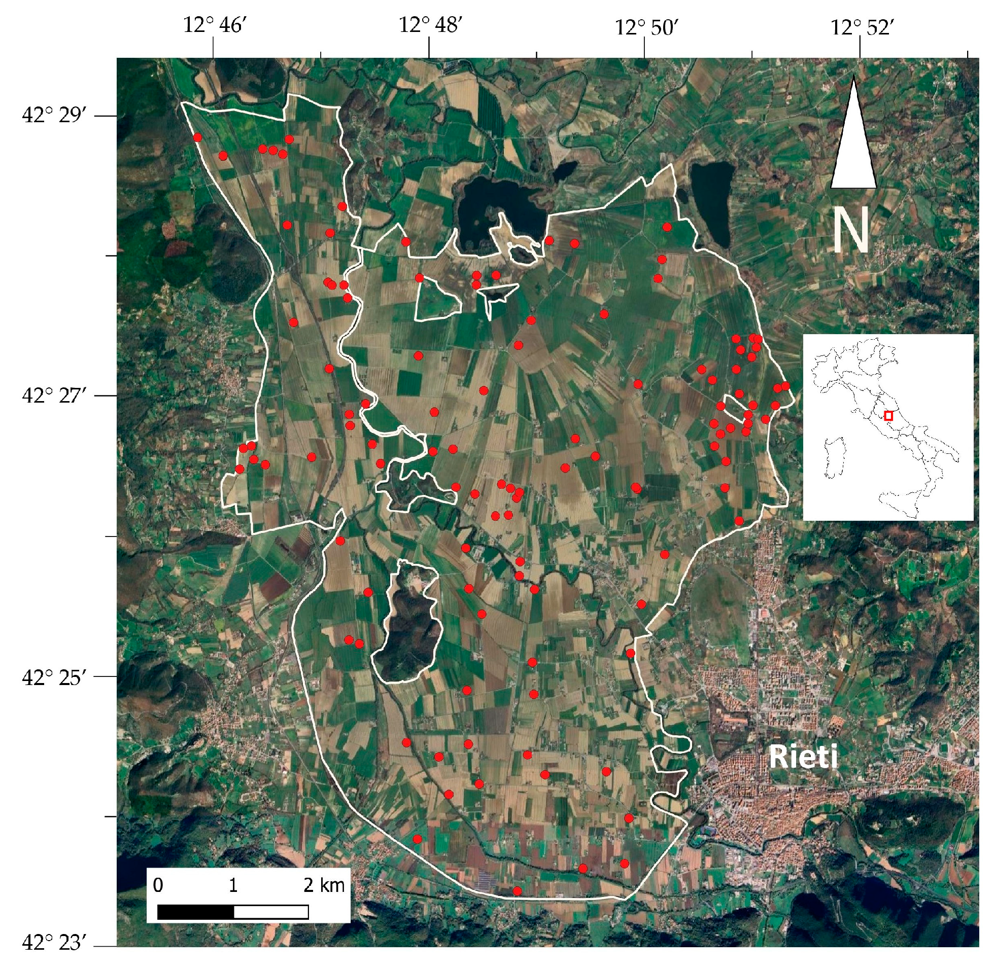
The study area (Figure 1) (about 5200 ha) is located in an intra-mountain plain of Central Italy in the province of Rieti (around 42°26′N; 12°49′E). The area is bounded on the North and on the East by the Reatini Mountains, with the highest elevation being Mount Terminillo (2217 m a.s.l.), and on the South and West by the Sibillini Mountains (2476 m a.s.l. at Mount Vettore). The plain has a very slight slope gradient from South to North, with a slope always below 2%, and slightly higher gradients (<10%) on some edges of the lowlands, close to the slopes and elevations. The elevation of the study area ranges from about 420 m a.s.l. in the South and along the borders to about 360 m a.s.l. in the Northern part. Two rivers cross the plain, the main river Velino from South-East to North, and its tributary, the Turano river, from South-West to North. The mean annual temperature is around 10 °C, and the mean annual precipitation is around 1000 mm per year.

The Rieti plain is composed of Plio-Quaternary alluvial and lacustrine sediments and is bordered by reliefs composed of detritic, calcareous, and marly deposits. In prehistoric times, the Rieti basin was entirely occupied by a large lake fed by the Velino and Turano. The waters of the Velino, rich in calcium carbonate deriving from the alteration of the sedimentary rocks present along its course, began to sediment limestone, which collected particularly at the confluence point between the Velino and Nera rivers, creating a considerable difference in the height between the Rieti plain and the surrounding area, which were originally on the same level. The entire area was progressively reclaimed from the Roman time until the beginning of the XX century. In the early 1900s, two dams were built on the main tributaries of the Velino, the Salto, and the Turano, which would allow for the regulation of the flow of water from their respective catchment areas.

During the last century, the entire plain has become an important cropland area, with a cultivated surface of about 5200 hectares and several tens of farms. The main crops follow a rotation of durum wheat–sunflower in the Northern part of the plain, and corn–sunflower–sorghum in the Southern part. The main soil tillage systems (Ap layer) are inversion ploughing (30–40 cm deep) and non-inversion tillage or subsoiling (30–40 cm deep), followed by harrowing for sowing. A limited fraction of the land is used for permanent crops such as pastures or meadows.

A few small, isolated hills are also present within the basin, and they are used for tree cultivation or fallow land. These hills and the areas with riparian vegetation of the two rivers were excluded from the mapping effort.

2.2. Soil Characterization and Sampling

Legacy data from 12 soil profiles, collected from 1980 to 2015, were acquired from a regional soil database, having been previously used for the soil map of the Latium region [45]. These legacy data reported the soil description, classification, and laboratory analysis, and they were included in the database of this work. Furthermore, data from soil surveys and monitoring carried out in 2022 and 2023 by the research unit of the University of Tuscia were also used. The soil survey included soil profiles and manual augering to characterize soil typologies and to analyze soil horizons. It is evident that the use of legacy data leads to greater errors in data harmonization, as some soil characteristics may have been modified (e.g., SOC and TN), and the analysis may have been carried out in different laboratories. On the other hand, the use of legacy soil data is highly recommended to make soil mapping cost effective.

Profiles were described by conventional soil description methods and classified using international WRB classification [46]. A and B horizons were also collected for soil laboratory analysis. Manual augering was performed to a depth around 70 cm and was also described and classified following the WRB guidelines [46]. In manual augering, A horizons were consistently collected for laboratory analysis, whereas B horizons were only collected in certain instances. The results of this survey were aimed at producing soil typological units map (STUs) with traditional pedological methods.

Overall, 103 sites were sampled, and A horizons (usually 0–30/40 cm) were collected and analyzed using standard laboratory methods. Subsoil samples of B horizons were collected and analyzed at only 68 sites. Laboratory analyses were carried out in a certified laboratory, following standard Italian soil analysis [47,48]. In particular, texture analysis was carried out using a pipette method, according to USDA textural thresholds; the pH and EC were measured at a 1:2.5 soil/water solution; soil organic carbon (SOC) and total nitrogen were measured using the Wet methods of Walkley–Black and Kjeldhal, respectively; total carbonates were quantified using the gas-volumetric method of Dietrich–Fruhling using a calcimeter; and the cation-exchange capacity and exchangeable bases were measured via extraction in 1 N ammonium acetate solution. In addition to soil description and analysis, soil profiles and augering have been classified according to the World Reference Base Soil Classification [46] and grouped into soil typological units (STUs) according to their characteristics and pedogenetic processes.

2.3. Covariates

The soil characteristics within the entire study area were interpolated using non-stationary geostatistical methods, which included grids of explanatory variables, also known as covariates. In particular, two groups of covariates were selected: (i) morphometric indicators, based on a digital elevation model (DEM), and (ii) indicators based on multispectral remote sensing images.

2.3.1. Covariates from Digital Elevation Model

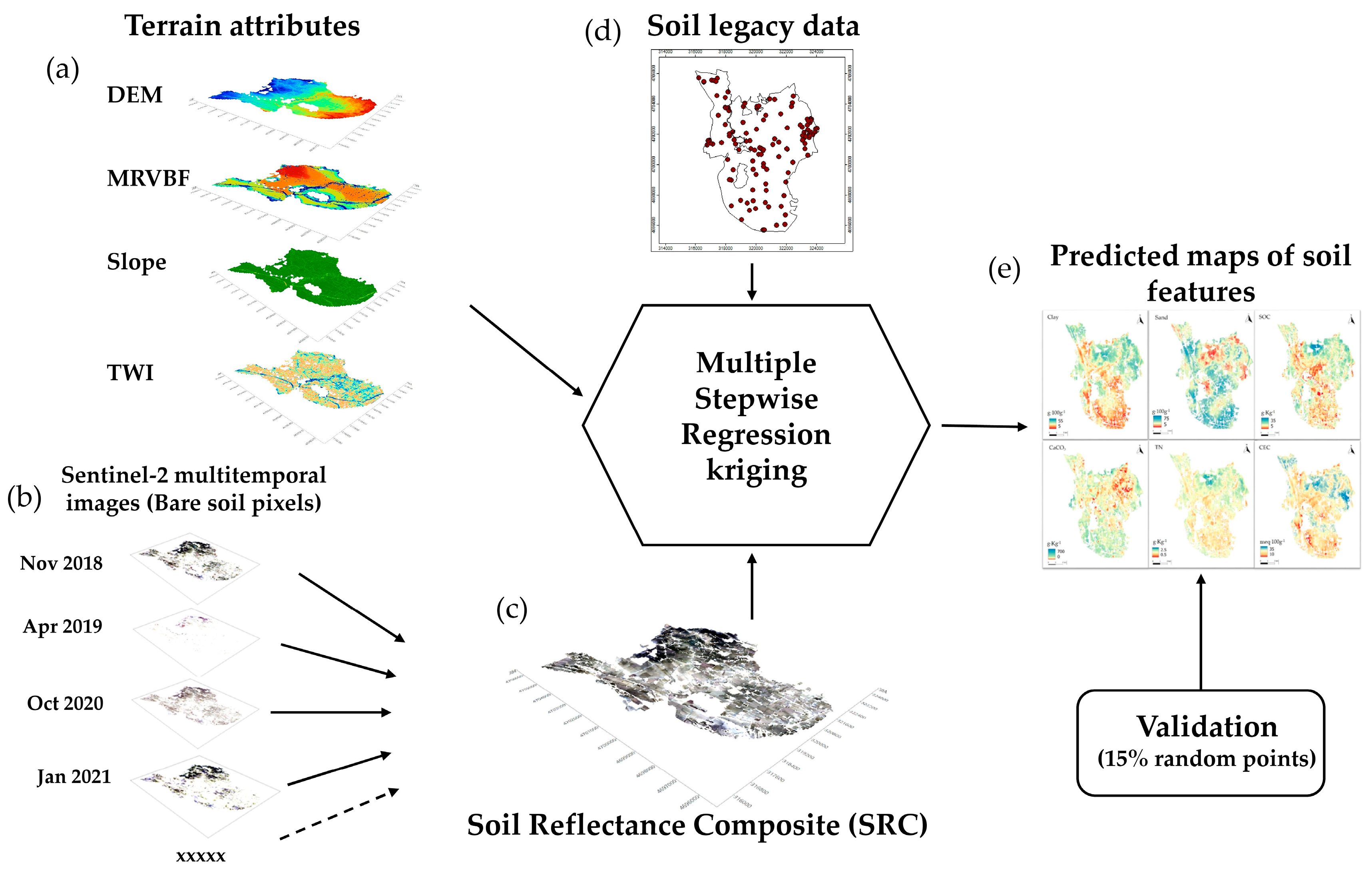
The study area was located within an enclosed plain between mountains, resulting in a predominantly flat surface. On the other hand, a clear elevation gradient was evident from the Southern part of the area (average elevation of 380–385 m a.s.l.) to the Northern part (average elevation of 360–365 m a.s.l.), exhibiting an average northward slope of −0.02%. An elevation grid (DEM) with a resolution of 5 m was downloaded from the map portal of the Latium region. The DEM covariates were calculated using SAGA-Gis 9.0, and they were the slope, Topographic Wetness Index (TWI), and Multiresolution Index of Valley Bottom Flatness (MRVBF). The reason for using the slope in a predominantly flat area was to distinguish the boundaries of the plain, characterized by a slight slope, from the rest of the internal plain (Figure 2a).

The TWI is one of the most widely used hydrologically based topographic indices and is a measure of the tendency of each cell to accumulate surface water, assuming uniform soil properties [49]. Areas prone to water accumulation (large contributing drainage areas) and characterized by low slope angles are associated with high TWI values. On the other hand, steep and convex slopes are considered well-drained areas and are associated with low TWI values [50].

The MRVBF (Multiresolution Index of Valley Bottom Flatness) utilizes the flatness and lowness characteristics of valley bottoms. Flatness is measured by the inverse of the slope, and lowness is measured by a ranking of elevation with respect to a circular surrounding area [51]. Values approaching zero identify regions exhibiting a relatively gentle slope, whereas higher values indicate areas of greater flatness and depression. Such a morphometrics index has been used by several authors working on digital soil mapping [52,53,54]. This is due to the capacity of this index to effectively differentiate between the extremely flat and depressed areas of the valley bottom, where sedimentation is at its maximum and the probability of waterlogging is higher than that in the relatively gentle slope of the distal plain.

2.3.2. Multitemporal Sentinel-2 Bare Soil Reflectance Mosaic

A multitemporal Sentinel-2 composite of bare soil reflectance was also used as a covariate. Sentinel-2-MSI satellite data, processed to bottom-of-atmosphere reflectance using the MACCS-ATCOR Joint Algorithm (MAJA) [55], were used for this work. The Sentinel-2 MultiSpectral Instrument (S2-MSI) mission was launched by the European Space Agency (ESA) in 2015. Two satellites (2A and 2B) were placed in orbit, providing a five-day revisit time. Sentinel 2-MSI has spatial resolutions ranging from 10 to 60 m and thirteen spectral bands covering the visible, near-infrared, red-edge, and short wave-infrared regions. To obtain a mosaic of the multitemporal bare soil reflectance of Sentinel-2 images, two main steps were followed:

• Pixels with cover, namely vegetation and crop residues, must be removed from each single-date Sentinel-2 image (Figure 2b).
• The SRC map is computed as a result of the means of each single-date Sentinel-2 image after removing the cover (Figure 2c).

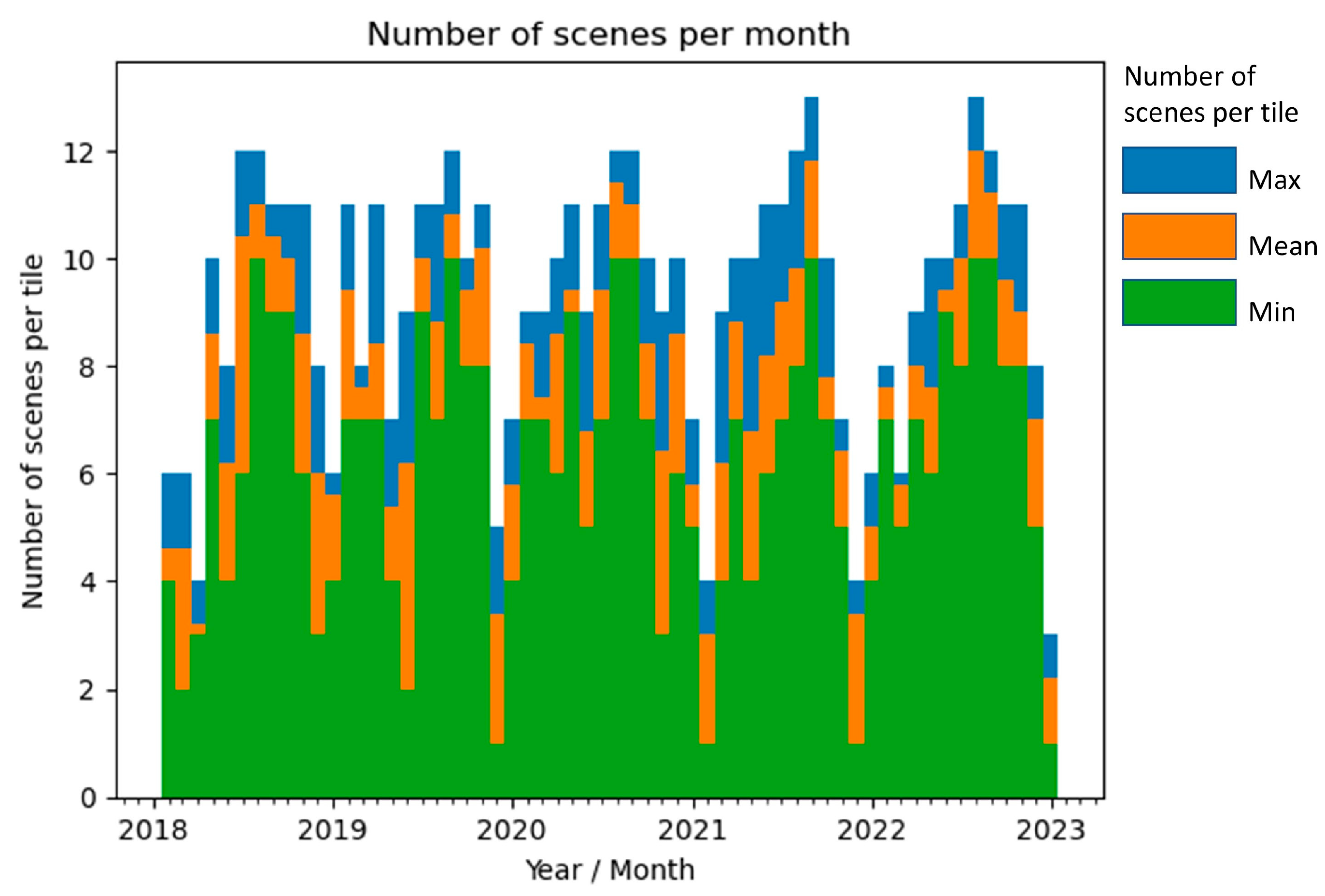
In particular, for generating the SRC, all Sentinel-2 scenes that were available in a five-year period between 2018 and 2022 covering the Rieti plain were included (Figure 3). The dataset included full-year data, as the area in question was cultivated with different crops during both the winter and summer months, causing the bare area to fluctuate throughout the year. This included data from 5 UTM tiles (32TQM, 32TQN, 33TTG, 33TUG, and 33TUH). The resulting data stack has been reduced by filtering out all scenes with a cloud coverage of >80%, sun elevation <20°, all bands (B1, B9, and B10) with a 60 m spatial resolution, and pixels classified as water, clouds, snow, and topographic shadows by the geophysical mask (*MG2-a product of MAJA processing). All Sentinel-2 bands with a pixel resolution of 10 m (B2, B3, B4, and B8) and SWIR bands (11 and 12), originally at 20 m resolution, were resampled at 10 m using B-spline interpolation by SAGA-Gis 9.0.

For the bare soil pixel selection, the PV+IR2 index [55] combining the NDVI and NBR into one index is used. Thresholds are derived per UTM tile using the HISET methodology, using crop and grassland areas from the ESA WorldCover map [56]. For each Sentinel-2 scene, these surface reflectance pixels are stored in a temporal data stack below the PV+IR2 index thresholds (0.12–0.21). Pixels containing the remaining cloud and haze effects are filtered out in two ways: (1) sB12 − sB8 > 0, where s is the surface reflectance of the respective band B, and (2) filtering outliers in the blue band (B2) in relation to the median of the dataset in the blue band (Karlshoefer et al., in review). On a per-pixel basis, the SRC map is created by calculating the average of bare soil pixels extracted from each band of Sentinel-2 images. A minimum of 19 and a maximum of 391 pixels are used to calculate each pixel of the SRC map.

2.4. Soil Data Interpolation

A preliminary investigation on the relationships between soil features and covariates was carried out using Spearman’s correlation.

The entire dataset of soil profiles and augering details (n = 115) was subdivided into calibration (85%, n = 98) and validation datasets (15%). The validation sites were randomly selected, extracting 17 sites (≈15%) from the general dataset and removing them from the map interpolation procedures. The predictive models of subsoil features (clay_sub, sand_sub, and CaCO₃_sub) used only 68 data points: 57 for calibration and 11 for validation.

The soil features used for interpolation were clay, sand, total lime (CaCO₃), soil organic carbon (SOC), total nitrogen (TN,) and the cation-exchange capacity (CEC).

The normality of the data was evaluated using histograms and the Kolmogorov–Smirnov test. The data for CaCO₃, SOC, and TN exhibited a distinct non-normal distribution; therefore, data normalization procedures were also performed to verify eventual improvements in regression kriging prediction.

The “OrderNorm” function of the “BestNormalize” package in R [57] was used for the normalization of CaCO₃ and TN, whereas the “Arcsinh” function was used for SOC.

The spatialization of the soil variables was carried out using regression kriging (RK) with forward stepwise multiple linear regression (Figure 2), using SAGA-Gis 9.0 software [58]. The covariates used for this geostatistical method were the DEM, DEM covariates (slope, TWI, and MRVBF), and the ten bands of Sentinel-2, produced via SCMaP, namely band 2 (blue), band 3 (green), band 4 (red), band 6, band 7, band 8 and 8a (NIR), and bands 11 and 12 (SWIR).

RK is a geostatistical technique that combines a regression of the dependent variable on auxiliary variables (or covariates) with simple kriging of the regression residuals [59]. Regression is used to model the spatial variation that is correlated to one or more explanatory variables (deterministic components), whereas kriging of residuals is used to model the unexplained variation (stochastics components).

This geostatistical method is applicable in most cases where the number of soil sampling points is relatively small and there is a statistically significant correlation between the soil properties measured at these points and one or more auxiliary variables. Multiple linear regression was used to model the relationships between soil features and covariates. To prevent the inclusion of insignificant or redundant variables in the multiple regression and then model overfitting, a forward stepwise approach was selected. The forward stepwise approach starts with the null model and subsequently incorporates a variable that optimizes the model, one at a time, until a pre-established stopping criterion is met. The criterion for the inclusion of a predictor in the model is based on the F-statistic and, in this case, is associated with a p-value of 0.05. The quality of multiple regression was assessed by inspecting the R²_adj and RMSE (Root Mean Square Error). In this study, the residuals were interpolated via ordinary kriging, after semi-variogram modeling. The sum of the maps of regression estimates and the maps of residuals interpolated via ordinary kriging provided the final maps of the predicted soil features (Figure 2e).

RK has been widely applied in digital soil mapping [60,61,62] and has often shown better performance than ordinary kriging, co-kriging, as well as machine learning methods [63,64]. A recent review [65] reported that most of the digital soil mapping using the RK approach covered the local scale, which is also the scale of this work.

The validation of the interpolated maps was carried out by 17 randomly selected soil augering points, which were extracted by the dataset and not used in the RK calibration procedures. The validation procedure calculated the RMSEP (Root Mean Square Error of Prediction), the coefficient of determination (R²) between the predicted and the measured values, and the Ratio of Performance to InterQuartile distance (RPIQ). The latter is calculated as the interquartile range (Q75–Q25) of the observed values divided by the RMSEP.

2.5. Mapping the Soil Typological Units (STUs) by Supervised Classification

A supervised classification method to map the distribution of the soil typological units (STUs), which were previously identified and classified using the soil survey, was also tested using SAGA-GIS. The soil observations (profiles and augering data) that were classified and attributed to an STU were used to calibrate the classification model. A 20 m round buffer was created around each soil observation point, transforming the point shapefile into a polygon shapefile. The explicative layers used for classification were the terrain attributes (DEM, slope, MVRBF, and TWI), SRC bands, and all predicted maps of soil properties (clay, sand, clay_subsoil, sand_subsoil, CaCO₃, SOC, TN, and CEC), performed in the previous step. The predicted maps of the soil parameters of subsoil horizons (B horizons) were only clay_sub and sand_sub. Two new maps, representing the differences between clay in A horizon versus clay_sub and sand in A horizon versus sand_sub, were also produced to highlight eventual lithological discontinuities. In fact, such lithological discontinuities were typical of an STU, namely REO, described in the following section.

The method selected for classification was the supervised classification for grids and polygons, using an artificial neural networks approach called “Winner Takes All” (WTA). WTA is a competitive machine learning strategy, often used in image classification [66,67]. This computational technique tests several classification models and, for each pixel, uses the model with the highest activation value, which is the result of the non-linear activation function used from each model. SAGA-GIS simultaneously compares 6 classification models: (i) Binary Encoding, (ii) Parallelepiped, (iii) Maximum Distance, (iv) Mahalanobis Distance, v) Maximum Likelihood; and vi) Spectral Angle Mapping.

Three datasets of covariates were tested for this supervised classification: (1) terrain attributes and SRC bands; (2) predicted maps of the single soil features, including clay and sand of subsoil, and the ratio between topsoil and subsoil for clay and sand; and (3) all the available covariates (terrain attributes, SRC bands, and predicted maps of soil features).

A confusion matrix between STU maps and the sampling points was carried out to evaluate the accuracy of each classification method.

3. Results

3.1. Soils Features and Statistical Correlations

Legacy data from the different soil surveys showed sandy and clayey soils developed on Plio-Quaternary alluvial and lacustrine sediments, with little or no stoniness. The classification of soil observations, already reported in the legacy data, was revised, according to the new WRB classification [45], and included three reference groups: Cambisols, Phaeozems, and Vertisols. Five soil typological units (STUs) were identified, as described in

Table 1. Soil typological units and WRB classification of the soil observations within the Rieti plain.

STU	Classification (WRB, 2022)	Textural Class	n.observ.
LLU	Haplic Vertisols (Calcaric)	clay, clay–loam	19
REO	Haplic Vertisols (Calcaric, Raptic) or Calcaric Cambisol (Loamic, Raptic)	clay–loam over sandy–loam	11
MONT	Calcaric Cambisols (Loamic)	loam, clay–loam, sandy–clay loam	49
TUR	Eutric or Calcaric Cambisols (Arenic)	sandy–loam, loamy–sand	17
RIPA	Endo-Calcaric Phaeozems (Loamic)	clay–loam, clay	6

. The most common STU is MONT, which included Calcaric Cambisols (Loamic) developed on the alluvial deposits of the Velino river and colluvial–alluvial deposits around the border of the plain, generally at an altitude between 375 and 380 m a.s.l. Such an STU is characterized by a loam or clay loam texture, scarce or no stoniness, good drainage, and scarce horizonation. The STU TUR is very similar to the previous one, but with sandy loam, loamy sand, or, in only one case, sandy texture.

In the Northern part of the plain, which is slightly more depressed (360 m a.s.l.), the most common STU was LLU, characterized by Vertisols generally calcareous and with stagnic or gleyic properties in depth. In the same Northern area, soils with no vertic properties, but a clay or clay–loam texture and gleyic or stagnic properties in depth, were also individuated. These soils were attributed to the STU RIPA and classified as Phaeozems.

In the Northern-Central part of the area, another STU has also been found, namely REO. This STU showed a peculiarity, which is an evident lithological discontinuity between a clay or clay loam texture in the topsoil and sandy loam or loamy sand in the deeper horizons (>50–60 cm). The variability in physical and chemical soil parameters is probably influenced by the alluvial and lacustrine origin of the sediments in the plain. The presence of alternating clay and sandy deposits suggests an irregular deposition history, which has contributed to the observed differences in the soil properties, particularly in the distribution of clay and sand, as also evidenced in the B horizons. The variability in the total CaCO₃ content, with values reaching up to 900 g∙kg⁻¹ in the subsoil, reflects the calcareous nature of the deposits, particularly highlighted in calcareous STUs such as MONT and LLU.

By analyzing the topsoil, we found that the soil particle distribution followed a trend from clay, clay–loam, loam, and sandy clay–loam. In general, clay showed the highest values (35–50%) in the Northern side of the plain and the lowest in the Southern side (5–20%,

Table 2. Descriptive statistics of soil variables used in the spatialization of analyzed samples (_sub is referring to the subsoil; all the other variables are referring to the topsoil).

	n	Mean	Min	Max	St. Dev.	Skewness	Kurtosis
Clay	115	28.6	5.0	56.0	11.0	0.1	−0.7
Clay_sub	68	28.5	3.0	56.1	12.5	0.1	−0.6
Sand	115	36.9	2.4	81.0	17.0	0.1	−0.7
Sand_sub	68	38.7	0.0	94.0	19.7	0.3	0.1
CaCO3	115	151.5	0.0	755.0	117.0	2.2	7.1
CaCO3_sub	68	165.9	0.0	900.0	154.5	2.9	4.2
pH	115	8.1	7.0	8.5	0.2	−1.5	10.6
SOC	115	14.8	1.0	75.8	8.6	4	24.3
TN	115	1.6	0.1	9.0	1.1	4.2	20
CEC	115	22.7	7.1	39.5	7.4	0.3	−0.5

). The highest percentage of sand (50–80%) was mainly found in the observations closer to the rivers Velino (in the center of the plain) and Turano (in the South), in particular. As expected, the sand fraction has a negative correlation with clay (

Table 3. Spearman’s ranks correlation between soil properties. In bold, significant correlations for p < 0.001.

n = 115 n(sub) = 68 p < 0.01	Clay	Clay_sub	Sand	Sand_sub	CaCO3	CaCO3_sub	pH	SOC	TN	CEC
Clay_sub	0.81
Sand	−0.88	−0.66
Sand_sub	−0.69	−0.81	0.84
CaCO3	−0.15	−0.01	0.18	0.09
CaCO3_sub	0.00	0.01	0.16	0.14	0.86
pH	0.07	0.00	−0.02	0.13	0.14	0.15
SOC	0.58	0.66	−0.57	−0.67	0.02	0.01	−0.19
TN	0.39	0.38	−0.34	−0.31	0.12	0.04	−0.17	0.74
CEC	0.84	0.63	−0.81	−0.63	−0.22	−0.15	−0.08	0.54	0.42

).

CaCO₃ also showed a large variability, with areas free of carbonates, being more frequent on the North side, and areas with amounts higher than 700 g·kg⁻¹ (Table 2). In this area, CaCO₃ was not statistically correlated with any of the other soil variables (Table 3). The pH was very homogeneous and sub-alkaline (8.1–8.5) all over the Rieti plain; therefore, this variable was not spatialized. Soil salinity, determine by electrical conductivity (EC) using a 1:2.5 solution, was always low from 0.1 and 0.35 mS·cm⁻¹, and it was also not used for spatialization.

SOC showed relative homogeneity, with mean values around 10–15 g·kg⁻¹, although some higher values (from 50 to 75 g·kg⁻¹) were present in the Northern area. This high content of SOC derived from the presence of lacustrine and palustrine sediments rich in organic matter and with thin peat layers, now generally mixed with the Ap horizons by tillage.

Total nitrogen (TN) showed moderate variability and high correlation with SOC (Table 3) and also showed few high values (around 9 g·kg⁻¹) in the Northern sites characterized by thin peat deposition.

CEC is positively correlated with clay, SOC, and TN and negatively correlated with sand (Table 3); therefore, it showed generally high values on the Northern side and lower values near the two rivers.

The B horizons have been generally analyzed only for texture and CaCO₃. They also have a large spatial variability, in some cases being linked to the spatial variability of the correspondent A horizons. In the case of the REO typological unit, the soil type exhibited abrupt textural changes, with the presence of sandy loam B horizons beneath clay loamy or loamy A horizons. For the rest of the soil observations, the trend of clay and sand contents in the subsoil is very similar to that of the topsoil. Total carbonates also show a wide variability in the subsoil, ranging from 0 to 900 g·kg⁻¹, but with a high correlation with topsoil CaCO₃ (Table 3).

Regarding the distribution of the values, clay, sand, and the CEC showed a quasi-normal distribution and a skewness ranging from 0.1 to 0.3. On the contrary, CaCO₃, SOC, and TN showed a positive skewness ranging from 2.2 to 4.2. For this reason, these variables were transformed by normalization procedures, and the spatialization was subsequently performed with both normalized and non-normalized values.

Both Pearson and Spearman correlations were tested, but since they provided similar results, only Spearman’s rank correlation was shown in this paper, particularly because some variables did not follow a normal distribution.

Spearman’s rank correlations showed weak relationships between soil properties and DEM covariates. In particular, the DEM was significantly correlated with clay, sand, SOC, TN, and the CEC (

Table 4. Spearman’s ranks correlation between soil properties and covariates. “b” corresponds to the Sentinel-2 bands. The number of samples for topsoil is n = 115 and for subsoil is n = 68. In bold, significant correlations for p < 0.01 are presented.

n = 115 n(sub) = 68 p < 0.01	DEM	MRVBF	Slope	TWI	b2	b3	b4	b5	b6	b7	b8	b8a	b11	b12
Clay	−0.51	0.00	−0.15	0.08	−0.63	−0.62	−0.64	−0.66	−0.68	−0.68	−0.69	−0.69	−0.68	−0.72
Clay_sub	−0.37	−0.18	−0.06	−0.11	−0.51	−0.51	−0.54	−0.55	−0.55	−0.56	−0.58	−0.58	−0.60	−0.66
Sand	0.37	−0.05	0.14	−0.11	0.52	0.50	0.52	0.54	0.55	0.55	0.57	0.57	0.57	0.59
Sand_sub	0.19	0.13	0.04	0.09	0.48	0.47	0.49	0.50	0.50	0.51	0.53	0.53	0.57	0.59
CaCO3	0.13	−0.33	−0.06	−0.06	0.34	0.30	0.28	0.28	0.28	0.28	0.28	0.28	0.27	0.24
CaCO3_sub	−0.16	−0.20	−0.14	−0.16	0.15	0.09	0.07	0.07	0.07	0.08	0.09	0.1	0.11	0.04
pH	−0.20	−0.10	0.06	−0.15	0.09	0.10	0.11	0.11	0.11	0.11	0.10	0.10	0.10	0.08
SOC	−0.38	0.05	−0.25	0.20	−0.48	−0.49	−0.50	−0.50	−0.50	−0.50	−0.51	−0.51	−0.48	−0.5
TN	−0.27	−0.03	−0.21	0.13	−0.36	−0.37	−0.39	−0.39	−0.40	−0.40	−0.40	−0.41	−0.40	−0.42
CEC	−0.39	0.05	−0.17	0.07	−0.61	−0.60	−0.61	−0.63	−0.65	−0.65	−0.66	−0.67	−0.68	−0.70

). CaCO₃ of the A horizon was significantly correlated with the MRVBF. On the other hand, all the Sentinel-2 bands of the SRC showed significant correlations with most of the soil variables, with the exception of pH and CaCO₃_sub (Table 4). In particular, clay, SOC, TN, and the CEC were significantly negatively correlated with all the SRC bands, whereas sand and CaCO₃ were positively correlated. It should be stressed that all the SRC bands were strongly correlated with each other (rs > 0.90) and, to a lesser degree, with the DEM (

Table 5. Spearman’s ranks correlation between covariates, extracted in the 115 sampling points. “b” corresponds to the Sentinel-2 bands extracted from the SRC index. In bold, significant correlations for p < 0.01 are presented.

n = 115	DEM	MRVBF	Slope	TWI	b2	b3	b4	b5	b6	b7	b8	b8a	b11
MRVBF	−0.10
Slope	0.38	−0.41
TWI	−0.09	0.49	−0.56
b2	0.55	−0.20	0.25	−0.15
b3	0.58	−0.19	0.24	−0.14	0.99
b4	0.57	−0.18	0.24	−0.13	0.98	1.00
b5	0.57	−0.18	0.24	−0.14	0.98	0.99	1.00
b6	0.58	−0.18	0.26	−0.15	0.98	0.99	0.99	0.99
b7	0.56	−0.17	0.26	−0.16	0.97	0.98	0.98	0.99	1.00
b8	0.56	−0.17	0.27	−0.16	0.97	0.97	0.98	0.99	1.00	1.00
b8a	0.56	−0.17	0.26	−0.16	0.97	0.97	0.97	0.98	0.99	1.00	1.00
b11	0.47	−0.17	0.26	−0.15	0.92	0.91	0.92	0.93	0.95	0.95	0.97	0.97
b12	0.51	−0.12	0.24	−0.12	0.93	0.92	0.93	0.95	0.96	0.96	0.97	0.97	0.99

). For these reasons, the multiple regression to predict soil parameters used a stepwise approach, which removes all the redundant variables.

3.2. Spatialization of Soil Variables

The results of the forward stepwise multiple linear regressions adopted by the regression kriging approach to predict spatialized soil variables are summarized in

Table 6. Explicative covariates used for the regression.

Original Values	Variable Name	R2adj
Clay	b12, b11, DEM	0.54
Clay_sub	b12, b8a, MRVBF	0.54
Sand	b12	0.32
Sand_sub	b12, b6	0.35
CaCO3	b2, b4	0.29
SOC	b3, b11, TWI	0.35
TN	b6	0.17
CEC	b12, b11	0.49
Normalized values
CaCO3	b2, b8	0.22
SOC	b6, TWI	0.29
TN	b11	0.22

. One of the most explicative variables is SRC_band12 (SWIR), which was selected in the multiple regressions of clay and sand (topsoil and subsoil) and the CEC. SRC_ band 11 (SWIR) was also explicative for the prediction of topsoil clay, SOC, and the CEC. SRC_band6 (Red edge) resulted in the best predictor for TN and the second-best predictor for sand_sub. SRC_band2 (blue) and SRC_band4 (red) were explanatory for CaCO₃ regression.

The regressions that showed the best performance in terms of R²_adj were the predictions of clay (top and sub) and the CEC, whereas the worst performance was shown for the TN prediction (R²_adj = 0.18). Although the subsoil texture cannot be predicted using remote sensing, which directly investigates only the soil surface, the prediction of clay and sand of the B horizon (clay_sub and sand_sub) was also tested to evaluate indirect relationships.

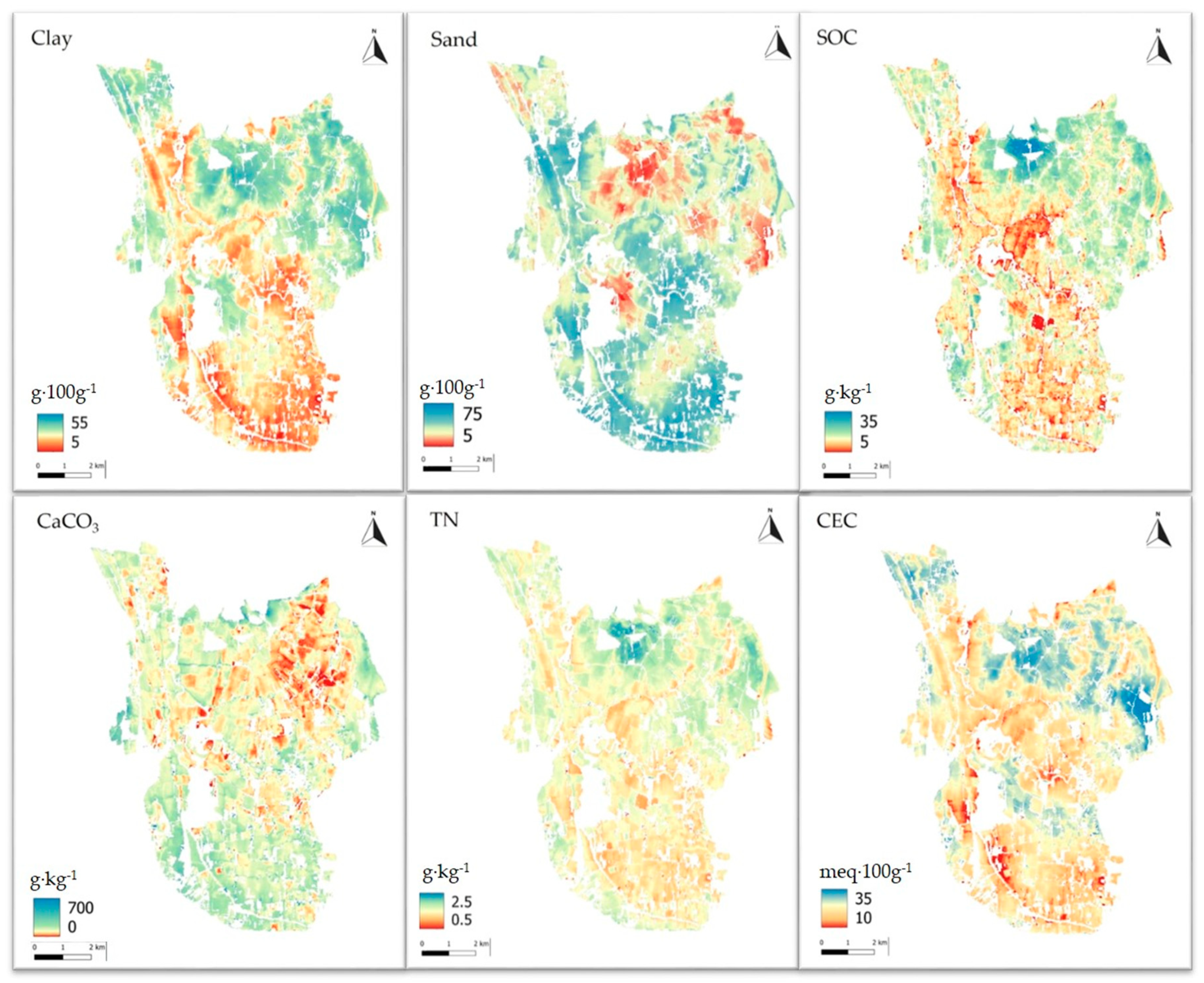
The regression results demonstrate that the SRC bands were the most valuable covariates for predicting soil parameters, including subsoil clay and sand, in the Rieti plain area. Interpolation via simple kriging of the regression residual, which is the second step of the RK procedure, was possible for all parameters because the spatial autocorrelation of the residuals could be modeled using a semi-variogram. The predicted maps of soil parameters are reported in Figure 4.

Apart from a slight improvement in the prediction of SOC, there were no significant improvements in TN and CaCO₃ despite normalizing the data. The performance of the regression was not greatly influenced by data normalization but rather by the correlation with the covariates.

3.3. Validation of the Results

The maps of soil variables predicted using RK (Figure 4) were validated using 17 soil observations that were randomly selected and removed from the previous mapping procedures. The means of the validation points (

Table 7. Descriptive statistics of the 17 validation points. The suffix “_sub” refers to the soil characteristics of the subsoil horizons (B horizons).

Variable		Mean	St. Dev.	CV (%)
Clay	g·100 g−1	29.6	9.1	30.9
Clay_sub		24.2	10.9	45.2
Sand		37.0	16.9	45.5
Sand_sub		43.3	25.4	58.7
CaCO3	g·kg−1	143.7	107.1	74.5
SOC		12.6	4.1	32.5
TN		1.4	0.4	28.0
CEC	meq·100 g−1	22.7	7.2	31.5

) were consistent with the variability of the soil within the Rieti plain (Table 2), and the coefficient of variation (CV) was generally higher than 30%. Therefore, the validation dataset can be considered representative of the soil variability in the study area.

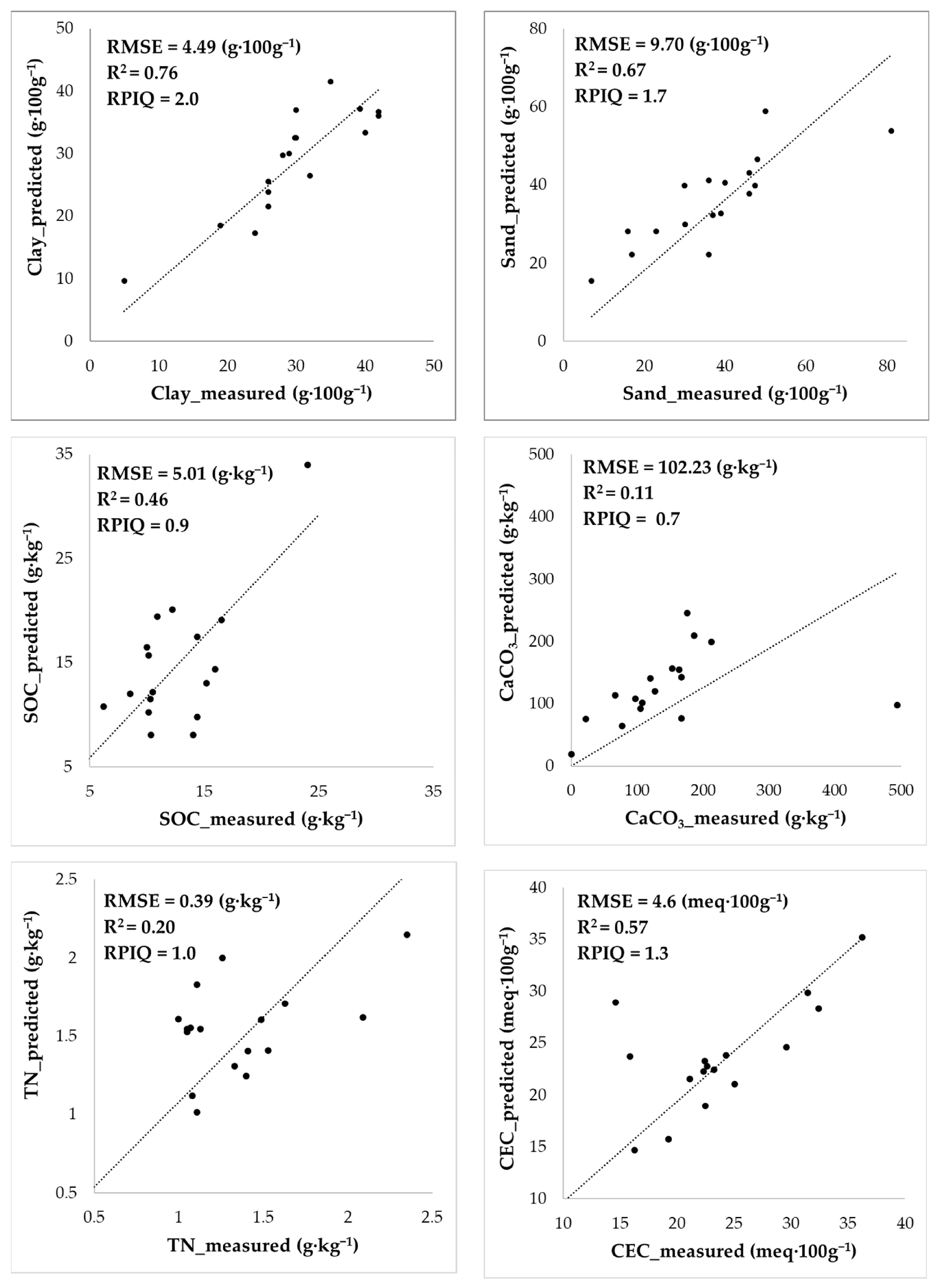
The results of the validation of the predicted map have been summarized in Figure 5 and Figure 6. The prediction accuracy was good for clay, sand, and the CEC, which showed a coefficient of determination (R²) ranging between 0.57 and 0.76. The prediction of clay showed the best accuracy, with an RMSE of 4.49 g∙100 g⁻¹ and an RPIQ of 2.0, whereas sand prediction showed slightly higher errors (9.7 g∙100 g⁻¹). The standard deviation of the measured values of sand was about twice that of clay (Table 7); therefore, the accuracy could be considered similar, as also demonstrated by very similar R² (0.67) and by acceptable RPIQ (1.6) values. The maps of the predicted subsoil parameters, namely clay_sub and sand_sub, were also validated in 11 points, instead of 17 of the topsoil maps, showing similar accuracy to those of the topsoil parameters. The R² between predicted and measured values was 0.70 and 0.50 for clay_sub and sand_sub, respectively, therefore being slightly lower than topsoil clay and sand prediction. The RMSEs were 5.6 g∙100 g⁻¹ for clay_sub and 17.2 g∙100 g⁻¹ for sand_sub. On the other hand, there was a strong correlation between the topsoil and subsoil textures, as reported in Table 3; therefore, the prediction model of the subsoil texture could be strongly influenced by the relationships between the topsoil texture and covariates.

SOC prediction showed limited results in terms of accuracy, with an RMSE of 5.01 g·kg⁻¹ and RPIQ of 0.9. Similarly, TN did not provide satisfactory prediction in terms of its R² (0.20), although the RMSEP (0.39 g·kg⁻¹) and RPIQ (1.0) were adequate. It is clearly observable in Figure 5 that one-half of the validation points fit almost perfectly with the bisector between predicted and measured, whereas one group showed higher errors of estimation, and another kind of correlation between predicted and measured. Probably, there is something influencing the TN distribution that we did not take into account. This could probably be due to fertilization and the temporal variation of TN in the soil, which is higher than the rest of the variables.

CaCO₃ prediction was the least satisfactory overall, with an RMSE of 102 g·kg⁻¹, R² of 0.1, and RPIQ of 0.7. This parameter showed a strong variability for the measured sites and a coefficient of variation of 74.5% for the validation sites. In Mediterranean areas, CaCO₃ in soils commonly shows very high spatial variability, varying from 0 to very high values according to the parent materials and soil hydrology context. The prediction model used in this paper for CaCO₃ tends to slightly overestimate the lower values (bias of CaCO₃ < 200 g∙kg⁻¹ = +5.5 g∙kg⁻¹) and strongly underestimate the higher ones (error of −396 g∙kg⁻¹ in a single point with CaCO₃ of 494 g∙kg⁻¹). Such large errors jeopardize the quantitative estimation of CaCO₃ but leave the possibility of distinguishing areas with no or low lime content from the others.

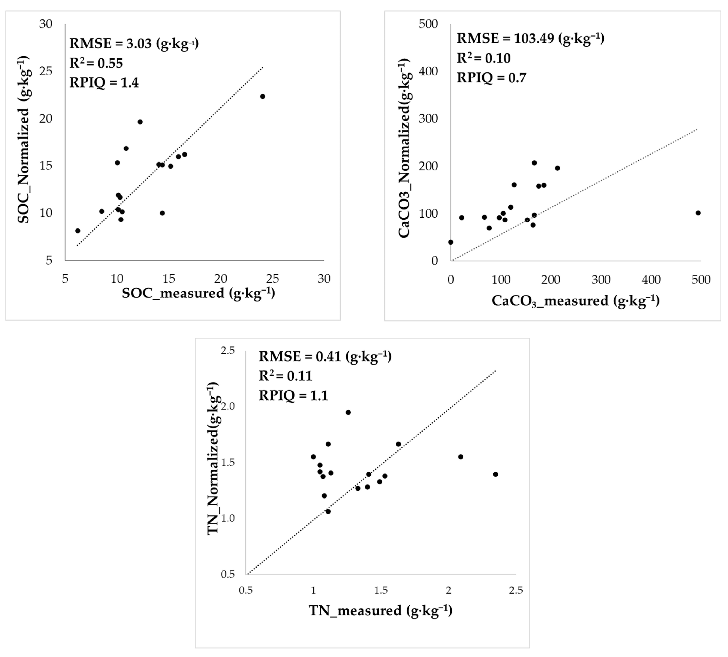
The normalization of the data with non-normal distribution, namely SOC, TN, and CaCO₃, before modeling did not show evident improvements in the accuracy, with the exception of SOC (Figure 6). The latter showed a decrease in the RMSE from 5.01 (non-normalized data) to 3.03 g∙kg⁻¹, a bias from 2.25 to 1.15 g∙kg⁻¹, and a satisfactory RPIQ of 1.4. High values of CaCO₃ were still predicted with strong underestimation, whereas low values were generally slightly overestimated. Therefore, validation confirms that the normalization of CaCO₃ data does not substantially enhance the results. This suggests that the underlying problem is the weak relationship between the target variables, namely TN and CaCO₃, and the predictors, rather than the non-parametric distribution of the data.

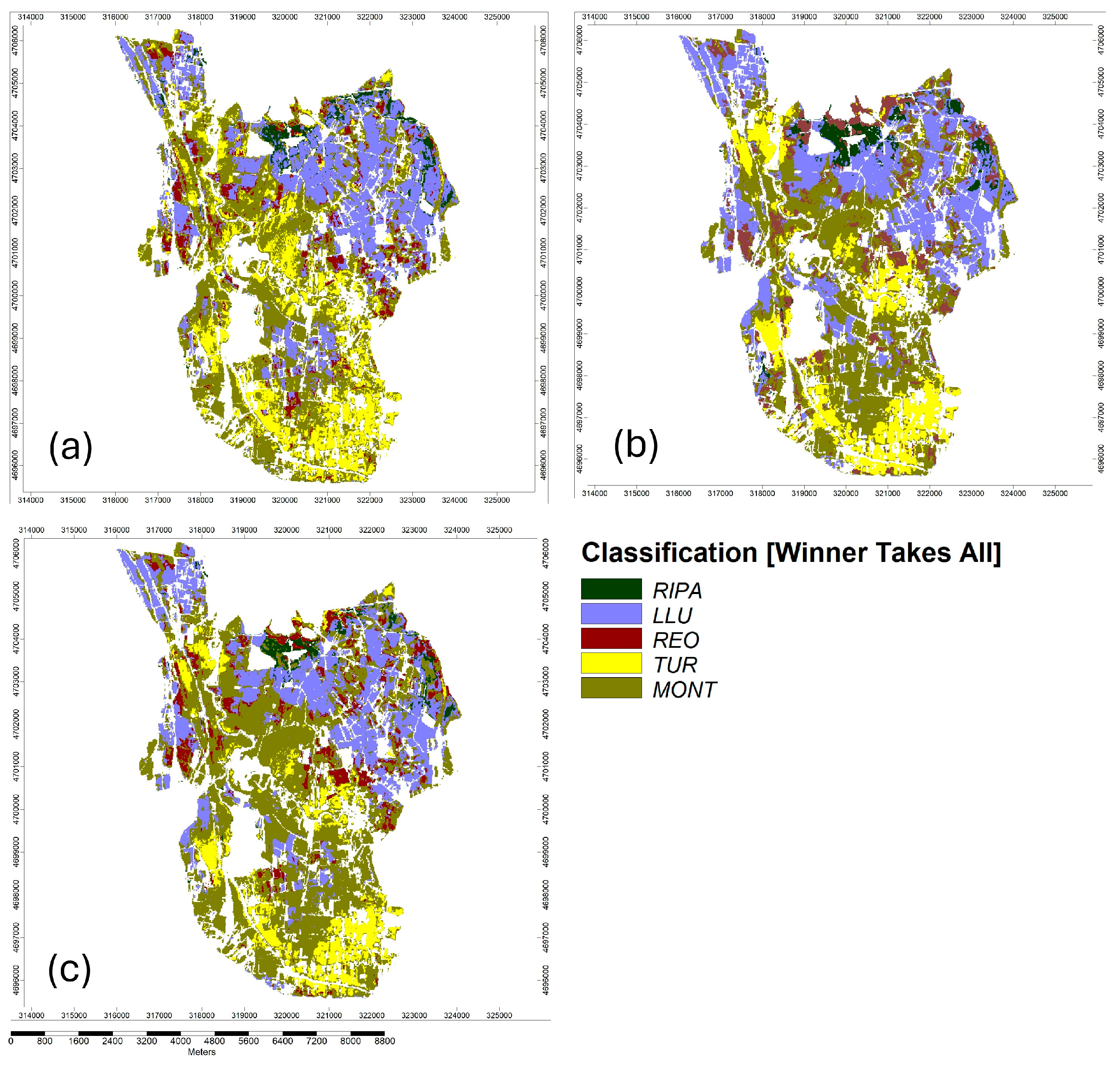
3.4. Map of Soil Typological Units (STUs)

The supervised classification of the terrain attributes, SRC bands, and predicted maps of the single soil features allowed us to obtain a categorical map of soil typological units (STUs) (Figure 7). The use of the WTA procedure allowed us to prioritize the best model of grid classification, improving the accuracy of the final map. The limited numbers of the sampling points, in particular for some less common STUs like RIPA, which had only six observations, make this classification not extremely robust. On the other hand, the results shown by the confusion matrices (

Table 8. Confusion matrix of the cross-validation of STU maps, using, as explanatory variables for the supervised classification, (a) only terrain attributes and SRC covariates; (b) only maps of the predicted values of soil features; or (c) both covariates and predicted maps. The row shows the pixels classified according to the field observations (sampling points with 20 m of rounded buffer); the column shows the pixels classified according to the supervised classification (WTA). The grey color highlights the right classification of the STUs.

(a) Terrain Attributes and SRC
		Described STUs					Accuracy	Overall Accuracy
Predicted STUs	STUs	LLU	RIPA	MONT	REO	TUR
	LLU	230	0	50	56	0	68%	76%
	RIPA	0	86	0	0	0	100%
	MONT	10	0	443	17	20	90%
	REO	11	0	39	69	4	56%
	TUR	0	0	115	13	205	61%
(b) Predicted Maps of Soil Features
		Described STUs					Accuracy	Overall Accuracy
Predicted STUs	STUs	LLU	RIPA	MONT	REO	TUR
	LLU	223	1	59	49	0	67%	79%
	RIPA	14	85	0	10	0	78%
	MONT	11	0	510	12	32	90%
	REO	3	0	35	65	4	61%
	TUR	0	0	43	19	193	76%
(c) Terrain Attributes and SRC + Predicted Maps of Soil Features
		Described STUs					Accuracy	Overall Accuracy
Predicted STUs	STUs	LLU	RIPA	MONT	REO	TUR
	LLU	247	0	46	55	0	71%	85%
	RIPA	0	86	0	0	0	100%
	MONT	4	0	563	16	20	93%
	REO	0	0	24	72	21	62%
	TUR	0	0	14	12	188	88%

) were very promising and showed an overall accuracy of pixel classification from 76%, using only the terrain attributes and SRC bands as covariates, to 85%, adding the predicted maps of soil features to the covariates.

In particular, the classifications of RIPA (Phaeozems) and MONT (Calcaric Cambisols) performed better than the others, probably for two different reasons. RIPA soil is located only in limited specific areas of the Northern part, characterized by flat surfaces slightly higher (about 1 m) than the rest of the plain. The terrain attributes and SRC bands allowed us to accurately map this type of STU. On the other hand, MONT is the widest and most representative (49 observation points, Table 1) STU of the Rieti plain, and it is mainly situated in the Central part of the basin.

The TUR STU mapping also performed well, in particular when the maps of soil features were used as covariates (Table 8b,c). In fact, this STU is very similar to MONT, and it is distinguished only by a sandier texture. The classification of LLU (Vertisols) and REO (Vertisols or Cambisols and Raptic) performed slightly worse, probably for several reasons. LLU is a rather abundant soil type in the Northern part (19 observations, Table 1), but the distribution is very heterogeneous. REO is the most complex STU because its main peculiarity is the lithological discontinuity between top- and subsoil (Raptic supplementary qualifier of WRB classification). In some cases, A horizons of REO were characterized by a clay or clay–loam texture, in other cases by a loamy texture. Therefore, the topsoil features were not discriminants for recognizing the REO STU. In addition, the spatial distribution of the REO STU was very discontinuous and probably follows ancient paleochannels active during palustrine environment and reclamation activities. However, using all the available covariates, including the ratio between topsoil and subsoil for clay and sand, allows us to obtain a rather accurate map of this STU (62% of pixel accuracy). Probably only proximal sensing methods, such as electromagnetic induction (EMI), can improve the accuracy and precision of mapping this soil type.

4. Discussion

The aim of this study was to test soil reflectance composite (SRC) indices coupled with terrain-based covariates for the digital soil mapping of an important arable territory in Central Italy, namely the Rieti plain. The soil data from the calibration (n = 98) and the validation (n = 17) sites were legacy data from previous studies and those collected in a recent soil sampling and surveying effort.

The Spearman rank correlations and the stepwise multiple regressions highlighted the high importance of the SRC indices for the prediction of all topsoil features investigated, namely clay, sand, CaCO₃, SOC, TN, and the CEC. In particular, SRC SWIR bands (b11: 1565–1655 nm; b12: 2100–2280 nm) showed the best performance in the prediction of clay, sand, the CEC, and SOC. In a flat area such as the Rieti plain, the terrain-based covariates showed less importance in the interpolation of soil characteristics than the SRC indices, although the DEM and MRVBF were explanatory for the clay and clay_sub maps, as well as the TWI for the SOC map. The significant improvement of the predictive model at a local field scale using the SRC in addition of terrain-based covariates has been also found by Moller et al. (2022) [68].

A recent paper [31] also found that Sentinel-2 SWIR bands (b11 and b12) showed the highest variable importance for SOC prediction. Similar previous works found consistent results, and most agreed that clay, the CEC, and SOC had the best predictive performance using multispectral imagery [25,26,69,70]. In a digital soil mapping study in four areas of the Czech Republic, Gholizadeh et al. (2018) [69] found that the relationships between Sentinel-2 bands and topsoil features were strongly site specific, although b12 often showed the best correlation with SOC and clay. In a Mediterranean environment, Vaudour et al. (2019) [25] found good correlations between Sentinel-2 multispectral images of bare soil and several soil parameters, in particular SOC and the CEC. In a study at a large, regional scale in Canada (Saskatchewan), Soreson et al. (2021) [71] used bare soil indices based on Landsat-5 and performed map predictions of SOC, clay, and the CEC, with prediction errors of 0.67 g∙100 g⁻¹ (R² = 0.55), 5 g∙100 g⁻¹ (R² = 0.44), and 5.7 meq∙100 g⁻¹ (R² = 0.50). At the field scale, in Brazil, Rizzo et al. (2020) [69] obtained R² values of 0.62 for clay content and 0.38 for organic matter content, using a multitemporal bare surface composite image based on the Landsat-5 satellite. In a recent work focused on the use of the SCMaP SRC to map SOC in Bavarian croplands, Zepp et al. (2021) [72] showed a map validation accuracy of SOC characterized by R² from 0.47 to 0.67 and an RMSE from 11.2 to 15.1 g∙kg⁻¹, according to the different algorithms used for the regression.

Most of these previous studies used Partial Least Squares Regression (PLSR) or machine learning methods, namely SVMs (Support Vector Machines), ANNs (Artificial Neural Networks), and RF (Random Forest) for digital soil mapping. For a limited number of sampling points for model calibration, like the 98 of this work, multiple linear regression to quantify the deterministic variation and ordinary kriging to quantify the stochastic variation have been preferred. On the other hand, there is not evident proof that machine learning methods or other geostatistical methods performed better, or worse, than RK, as reported by the review of Keskin and Grunwald (2018) [65]. According to this review, about one-third of the digital soil mapping papers using regression kriging for interpolation used factor analysis (PCA) to remove multicollinearity of covariates. In this work, forward stepwise regression was preferred to highlight the most important covariates for each dependent variable.

It is interesting to note that the data normalization of the SOC prior to the RK procedure did not result in a significant improvement in the linear regression performance (Table 6) but improved the accuracy of the final maps (Figure 5 and Figure 6). On the contrary, the normalization of TN and CaCO₃ did not show any improvement in the map prediction accuracy. It is known that skewed data, with important deviations from normality, affects linear regression. In addition, the residuals from the multiple regression analysis should have a low skewness to be interpolated via the kriging procedure. In this work, the skewness of the residuals showed similar trends of skewness as the original data, with values close to 0 for clay, sand, and the CEC and values from 1.3 to 3 for CaCO₃, SOC, and TN. On the contrary, the multiple regression analyses that use normalized values (CaCO₃_norm, SOC_norm, and TN_norm) also showed a quasi-normal distribution of the residuals and skewness varying from −0.01 to 0.22. From a geostatistical point of view, the normalization of CaCO₃, SOC, and TN was then correct, but the results, in terms of map accuracy, did not show clear improvements, with the exception of SOC. It should be emphasized that the multiple stepwise regressions on the normalized data used different covariates than on the non-normalized data (Table 6) and, in the case of SOC_norm, only one SRC band (b6) and not two (b3 and b11) as for the non-normalized SOC. Moreover, the regressions of normalized data did not improve their R²_adj, with the exception of TN_norm, which increased the R²_adj from 0.17 to 0.22. In other words, the statistical relationships between these soil variables and covariates were significant but moderate, as also shown by Spearman’s correlation (Table 4), and the normalization of the data did not improve such statistical relationships.

The results of this work showed that Sentinel-2 SRC bands, coupled with some terrain-based covariates, can be suitable auxiliary variables for digital soil mapping at the local scale in arable lands. The use of these freely available covariates and soil legacy data allows us to create high-detail topsoil maps at low cost for a medium or large agricultural district. In particular, the predicted maps of clay, sand, and the CEC showed excellent accuracies, determined via external validation. The result of SOC prediction was also fine, in particular using normalized data (SOC_norm). The CaCO₃ map showed higher errors (102 g∙kg⁻¹), in particular an overestimation of the lower values and a strong underestimation of the higher ones. On the other hand, the trend of the CaCO₃ map was consistent with reality, as shown by the validation plot (Figure 5). The results of this paper improved the map accuracy of a preliminary digital soil mapping effort for the Rieti plain, performed by the use of another index of bare soils, called a Synthetic Soil Image (SYSI) [44].

The prediction map of STUs, mapped as categorial variables using a supervised classification, showed acceptable performance. The only STU showing scarce results was REO because of its main peculiarities that were lithological discontinuity in depth, not observable in remote sensing images, and its fragmented spatial distribution. To map in detail such a soil type, which is characterized by subsoil horizon variation, other techniques are probably needed, for example, electromagnetic induction (EMI) sensing, as demonstrated in several papers [73,74].

Such work can be replicated in several other agricultural areas at a low cost, and the predicted maps can be very useful mainly for two objectives: (i) obtaining high-detail soil maps for precision agriculture; (ii) obtaining a baseline map of SOC of a certain agricultural territory to monitor the future evolution of SOC related to the modification of soil management or carbon farming practices, as also demonstrated in recent publications [75,76,77]. Regarding this last point, we must highlight that there are two limitations on the use of this approach to monitor the temporal variability of SOC or other dynamic soil features. The use of legacy data grouped the soil data collected at different times, providing a possible source of error due to the temporal variation of the soil feature. In addition, the use of an SRC covariate provides an image with average characteristics of the soil surface over several years. In a recent European-wide study [30], three consecutive 3-year bare SRCs were used to investigate the potential of SOC monitoring. The researchers concluded that the derived uncertainty level for croplands (P95 − P5 = 2.5 g C kg⁻¹) was lower than that required by the end users (5 g C kg⁻¹), which was defined in order to monitor SOC changes. The further reduction in the temporal length of the SRC to 1–2 years would result in a lower coverage of bare soil pixels and a reduced number of valid bare soil pixels, increasing the uncertainty of the soil reflectance spectra. Dvorakova et al. 2022 [23] found that a minimum of six observations is required to obtain reliable SOC content values. Future studies could be focused on the analysis of additional data characterizing the temporal variability of the soil spectral reflectance to improve the mapping and monitoring capabilities of soil properties.

5. Conclusions

This work aimed to produce a digital soil map of an important agricultural district in Central Italy, namely the Rieti intra-mountain plain, using soil legacy data, terrain-based covariates, and bare soil multitemporal composite images, namely an SRC, calculated using Sentinel-2 images. The work demonstrated that SRC Sentinel-2 bands, in particular SWIR (bands 11 and 12), can be outstanding explanatory variables to predict topsoil clay, sand, SOC, and the CEC. Other more heterogeneous and dynamic variables like CaCO₃ and TN showed a lower accuracy of prediction using this method, even if the prediction of semi-quantitative maps is possible.

The correlation between subsoil and topsoil textures, as well as between subsoil and some terrain-based covariates, allowed us to predict clay and sand of the B horizon. Using a supervised classification based on machine learning and using all the predicted maps of soil features, it was possible to obtain a map of soil typological units (STUs) with a classification accuracy of 85%, if all the covariates were used for the classification model.

The paper showed a case study that can be replicated in similar agricultural contexts, supporting the strength of the SRC, coupled with terrain-based covariates, in predicting maps of topsoil features and STUs. Although the predictive models used for this work, as well as the relationships between soil characteristics and covariates, may be site specific, the proposed approach can be replicated everywhere. It should be emphasized that the proposed method is indeed cost effective, as it uses existing soil data and freely available information layers such as the SRC and terrain-based covariates. The main limitation of using SRC imagery is that it requires bare, cultivated soil, at least for some periods of time. In soils that are always covered with grass or where no-tillage practices are used, it is not possible to use SRCs for digital soil mapping. In addition, the spectral mean obtained using SRCs provides an average multispectral topsoil image over several years, so the temporal variation of the soil surface during these years is lost.