CloudTran++: Improved Cloud Removal from Multi-Temporal Satellite Images Using Axial Transformer Networks

Abstract

We present a method for cloud removal from satellite images using axial transformer networks. The method considers a set of multi-temporal images in a given region of interest, together with the corresponding cloud masks, and produces a cloud-free image for a specific day of the year. We propose the combination of an encoder-decoder model employing axial attention layers for the estimation of the low-resolution cloud-free image, together with a fully parallel upsampler that reconstructs the image at full resolution. The method is compared with various baselines and state-of-the-art methods on Sentinel-2 datasets of different coverage, showing significant improvements across multiple standard metrics used for image quality assessment.

1. Introduction

Cloud removal from satellite images is a crucial part of remote sensing tasks, especially for the production of composite mosaics covering a region of interest and the analysis of multi-temporal data, including, among others, change detection [1,2], detection of phenological events [3,4], semantic segmentation of remote sensing images [5,6] and land cover classification [7]. Nowadays, Earth observation data of high spatial and temporal resolution are available thanks to the commissioning of a large fleet of satellites continuously monitoring the Earth. However, a large proportion of the collected data cannot be used as they are affected by clouds. This proportion depends on the geographic location of the region, its climate characteristics, and the season.

Cloud removal methods can be divided into two main categories, namely, those taking advantage of the temporal evolution of the pixel values and those attempting inpainting/gap-filling of parts affected by clouds in a single image, with the former having the advantage of being conditioned on the history of each pixel, reducing the prediction uncertainty for the missing values. Deep learning methods have been developed for both these categories. For single-image cloud removal, the proposed methods typically employ generative adversarial neural networks [8,9] while more recent works on this task integrate the self-attention mechanism into the standard generative adversarial network architecture (e.g., [10,11]). Multi-temporal cloud removal methods on the other hand typically employ conditional generative models, such as ResNet and U-Net, enriched with (ConvLSTM) modules (e.g., [12,13,14,15]), while multi-temporal cloud removal methods based on denoising diffusion have recently been proposed [16]. As these methods capture both the temporal and spatial relations of the pixels, although more challenging and computationally intensive, they typically lead to significant improvements in the produced cloud-free images.

Transformer networks have pushed the state-of-the-art in numerous natural language processing [17], computer vision [18,19], and remote sensing tasks [20,21] due to their ability to model long-range dependencies. However, their application in image generation and especially in the multi-temporal case is quite challenging due to their quadratic dependence on the input size (i.e., number of pixels). We propose a novel method for cloud removal from multi-temporal satellite images based on transformer networks [17] that are based on the axial attention mechanism. Axial attention [22] significantly improves temporal and parameter efficiency by applying attention independently on each tensor axis, without sacrificing the model’s receptive field.

The contributions of this work are the following:

• we propose a memory-efficient transformer-based method for cloud removal from multi-temporal images based on axial transformers that produces high-fidelity cloud-free images, both for thick and thin clouds, without considering additional data modalities (e.g., SAR);
• we perform experimental evaluation on an in-house multi-temporal Sentinel-2A dataset, as well as two customized RGB versions (L1C and L2A) of the publicly available SEN12MS-CR-TS dataset [14];
• compared with our previous work [23], we further improve the training strategy by considering a discriminator for reducing possible outlying intensity values, and we offer a more thorough experimental evaluation, by considering further comparisons with state-of-the-art methods.

2. Related Work

Cloud removal methods can be divided into two main categories, based on whether they use context from the temporal evolution of the pixel values, like ours, or they attempt to generate content to fill the cloudy part in a single image.

2.1. Single-Image Cloud Removal Methods

Cloud-GAN [8] is a generative adversarial network which uses two generator and two discriminator networks. By employing a cycle consistency loss, the generator is restrained to map the input domain to the target domain and vice versa, producing an output that is as close as possible to the original input. The method does not require a paired dataset with cloudy and matching cloud-free images, nor any extra sources, such as SAR data.

SpA-GAN [9] utilizes a Generator called the spatial attentive network (SPANet) and a Discriminator which is a standard convolutional neural network. The generator employs a spatial attention mechanism with a local-to-global perspective to detect cloudy regions and better capture the relative context so as to produce results with higher fidelity.

SACTNet [24] consists of two networks: first, a transformer-based network with a content extractor to get context from the ground-truth and the cloudy image, a correlation embedding and a soft attention module to synthesize texture elements; second, a backbone generative adversarial network that utilizes a spatial attention mechanism in a recurrent style in order to obtain spatial information for the regions affected by clouds. This method gives state-of-the-art results in the RICE dataset [25] for thin and thick cloud removal tasks.

Cloudformer [10] effectively combines the advantages of a self-attention mechanism and convolutional layers for thin and thick single-image cloud removal. Smaller-scale features are acquired through convolutions in the shallow layers of the U-shaped architecture, while a windowed-based multi-head self-attention calculates dependencies on a larger scale in the deeper layers of the network.

Cloud-EGAN [11], motivated by the CycleGAN framework that consists of two generators and two discriminators, also proposes the integration of a CNN with the self-attention mechanism. While both discriminators follow the PatchGAN structure, generators adopt a UNet architecture like the previous work. The contributions of this method include a saliency enhancement module (SE) during encoding and decoding in order to generate enhanced hierarchical feature maps. Combining the SE module with a CNN-based and subsequently transformer-based high-level feature enhancement modules, Cloud-EGAN retains global features for the cloud-free image.

2.2. Multi-Temporal Cloud Removal Methods

The work that introduces the SEN12MS-CR-TS multi-modal multi-temporal cloud removal dataset [14], also proposes two multi-temporal cloud removal methods. The first, is based on a 3D convolution neural network that considers time-series of Sentinel-1 (SAR) and Sentinel-2 (optical) data to produce a single cloud-free image. The second is a sequence-to-sequence method, with a 3D encoder-decoder architecture in a U-Net style, that takes as input time-series of Sentinel-1 images and produces the corresponding time-series of Sentinel-2 images. Subsequent work [26] has further improved the quality of the produced cloud-free images by introducing an attention-based architecture and a formulation for multivariate uncertainty prediction.

In [15], a conditional Generative Adversarial Network (cGAN) and a Convolutional Long Short-Term Memory (convLSTM) are employed to extract spatio-temporal features from multi-temporal Sentinel-1 (SAR) and Sentinel-2 (optical) data, respectively. Finally, the extracted features are fused by a U-shaped convolutional neural network to predict the final output.

DecRecNet [27] considers a background representation, derived from the cloud-affected image and its corresponding cloud mask and a cloud-free temporal image as the foreground representation with inverted masking in order to create a single composite image. The latter is passed through a ground content radiation correction module (GCR) and an imaging environment radiation correction module (IER) with their corresponding loss functions. Although this method utilizes a temporal cloud-free image, it does not incorporate the temporal axis to capture the historical evolution per pixel.

In this work, instead, we propose a method employing transformer networks for reconstructing a cloud-free target image considering only a small number of previously acquired optical images of the same region.

2.3. Video Inpainting

Video inpainting is a closely related computer vision task. The authors of [28] propose the Learnable Gated Temporal Shift Module (LGTSM) which handles masked videos with 2D convolutions. This method models the spatio-temporal features, processing context from a variable number of temporal neighbors. In [29], transformer networks are employed for video inpainting via fine-grained feature fusion. Two task-specific modules are introduced which are used in tokenization and de-tokenization before and after transformer layers, enabling sub-patch level information interaction for addressing blurring in masked regions caused by patch splitting. In our work, by using axial attention, we avoid the problems related to patch splitting-based vision transformer networks.

3. Method

We aim at producing a cloud-free version of a target image $I_T$ given a stack of cloud-affected images $I_{1:T}$ for a certain temporal horizon T. Our method is based on the use of transformer networks [17], which are powerful learning based estimators. Transformer networks are autoregressive models, i.e., each sequence element they produce, apart from the input, is also conditioned on all previously generated outputs.

3.1. Axial Transformers

Considering that both the number of parameters and their computational complexity depends quadratically on the number of sequence elements, for images where sequences of pixels are considered, transformer networks can have prohibitively large model sizes. To address this issue, several solutions have been proposed ([30] provides a survey). In this work, we consider Axial Transformers whose basic building block is axial attention [22]. An axial attention block performs self-attention over a single axis (here, columns and rows of an image), mixing information along that axis while keeping it independent along the other axes. This helps to reduce the model complexity to $\mathcal{O}\left(n\sqrt{n}\right)$, where n is the total number of pixels, providing $\mathcal{O}\left(\sqrt{n}\right)$ savings. This is especially crucial for processing multi-temporal data that we consider here.

Models employing axial attention achieve a global receptive field by combining multiple axis attention blocks spanning different axes. The resulting autoregressive network models a distribution $p\left(x_{i,j}\right)$ over a pixel x at position $(i,j)$ by processing all the past context from $x_{i,<j}$ and $x_{<i}$ following the raster scan order. Each axial attention block is composed of a self-attention block passing through a feed-forward block consisting of a layer normalization and a two-layer network. During training, a masked axial attention block is employed to prevent the model from considering subsequent outputs.

A full axial transformer architecture is composed of an encoder, capturing context from individual channels and images, an outer decoder capturing context of entire rows, and an inner decoder considering context within a single row. Specifically, the encoder consists of unmasked row and column attention layers and makes each pixel $x_{i,j}$ depend on all the previous channels and images. The output of the encoder is used as context to condition the decoder. In this work, we follow the conditioning approach proposed in [31].

Regarding the decoder, its outer part consists of unmasked row and masked column attention layers and makes each pixel $x_{i,j}$ depend on all the previous rows $x_{<i}$. The output context is then shifted down by a single row in order to ensure that it contains information only from previous rows and not from its own. This context is then summed with the encoder context and used to condition the inner decoder. The inner decoder consists of masked row attention layers, capturing information from the previous pixels of the same row $x_{i,<j}$. The inner decoder embeddings are shifted right by one pixel, ensuring that the current pixel is excluded from the receptive field. The new output context is then passed through a final dense layer to produce logits of shape $H\times W\times V$, where V corresponds to the range of pixel values at each location.

Outputs of autoregressive models are produced by sampling a single pixel at a time, which is a particularly computationally expensive process as the whole network needs to be re-evaluated each time. Axial transformers enable the significantly more efficient semi-parallel autoregressive sampling where the encoder runs once per image, the outer decoder once per-row, and the inner decoder once per-pixel. The context from the encoder and outer decoder conditions the inner decoder, which generates a row, pixel-by-pixel. After generating all pixels in a row, the outer decoder runs to recompute the context and condition the inner decoder, to generate the next row. After all the pixels of an image are generated, the encoder recomputes the context to generate the next image.

3.2. Proposed Architecture

The complete architecture of the proposed CloudTran method is presented in Figure 1. While the efficiency gains achieved by using axial attention blocks are substantial, it is still challenging to build encoder-decoder models for images of increased resolution (e.g., $224\times 224$ or higher) as, besides increased model size, sampling becomes excessively slow for generating images with higher resolutions. 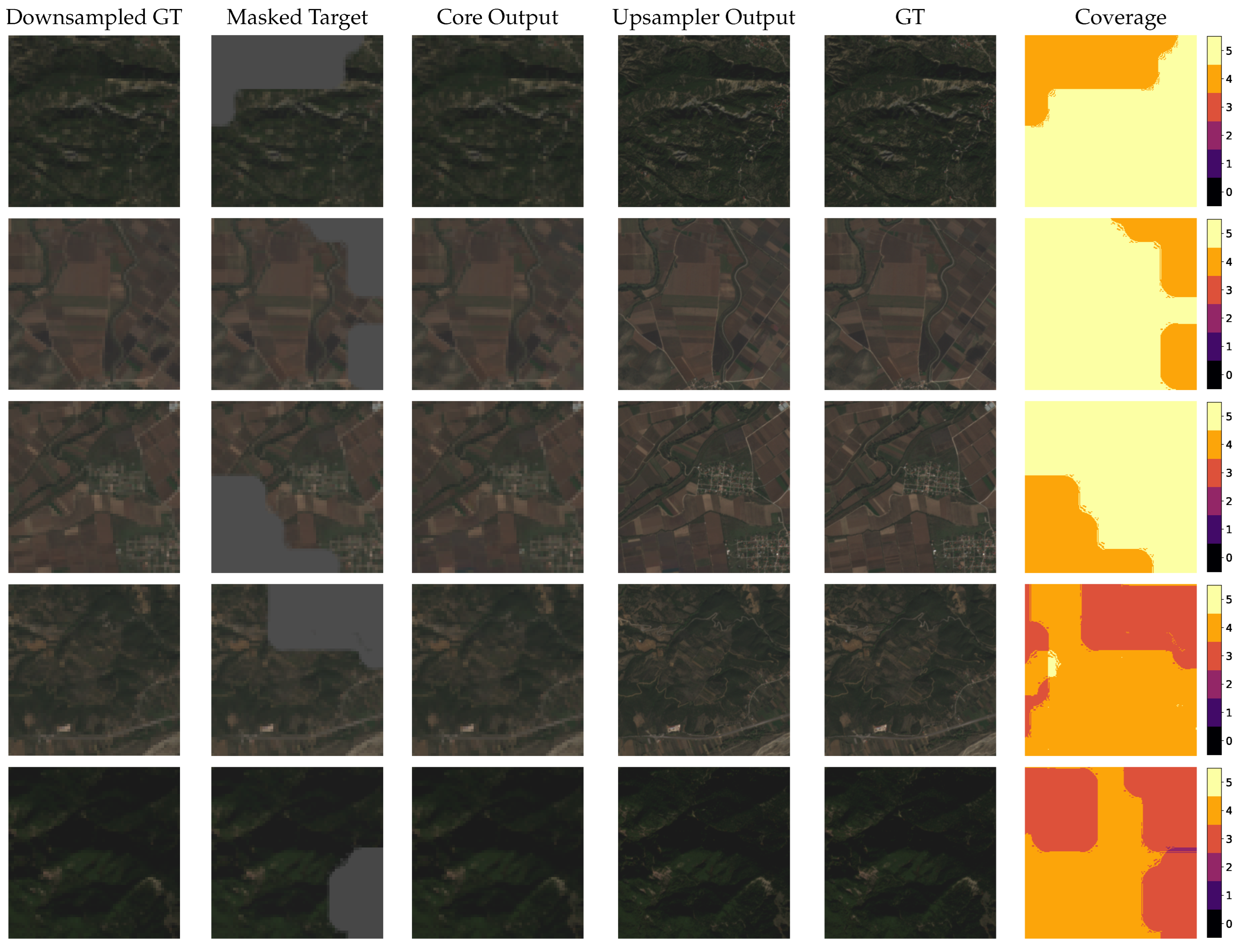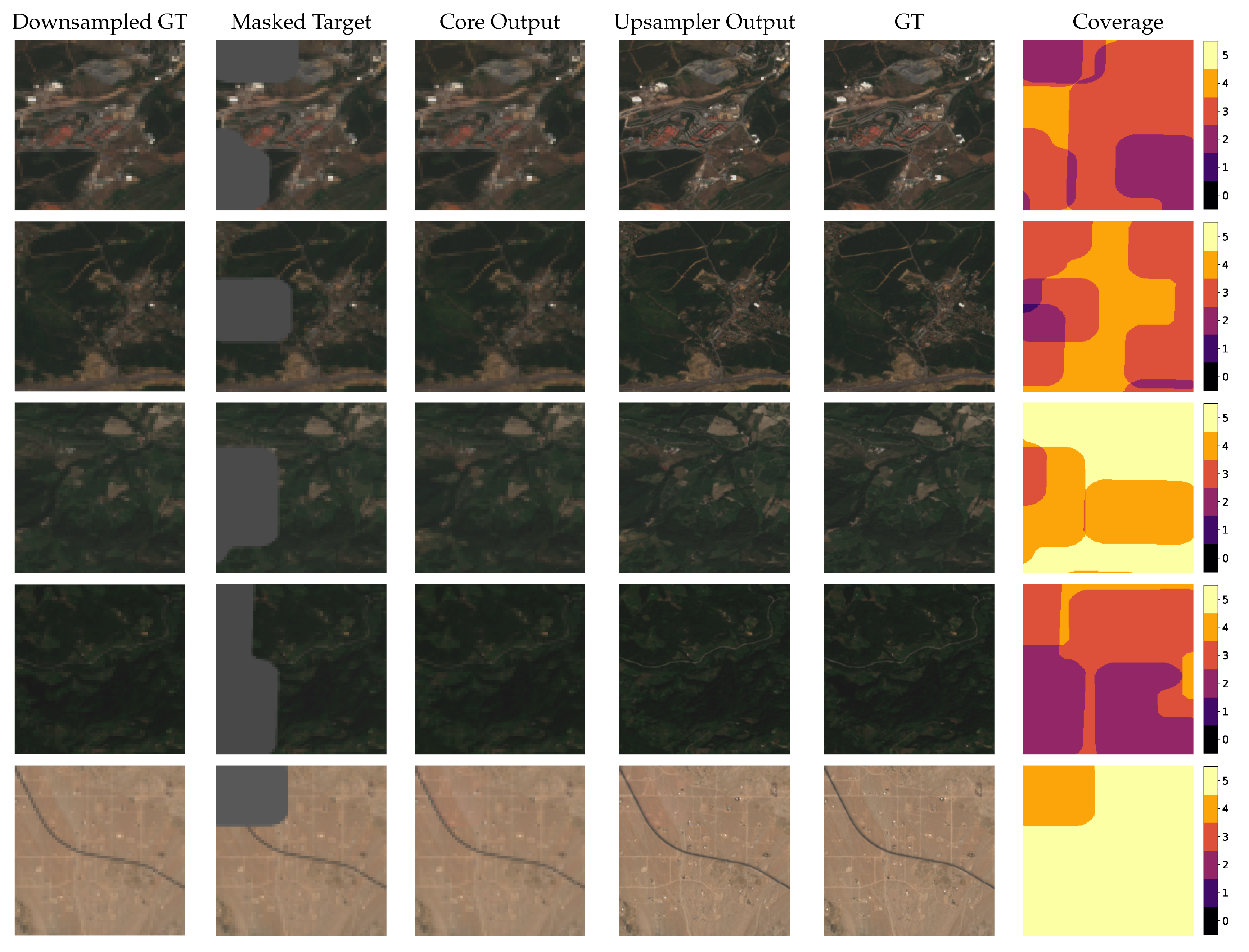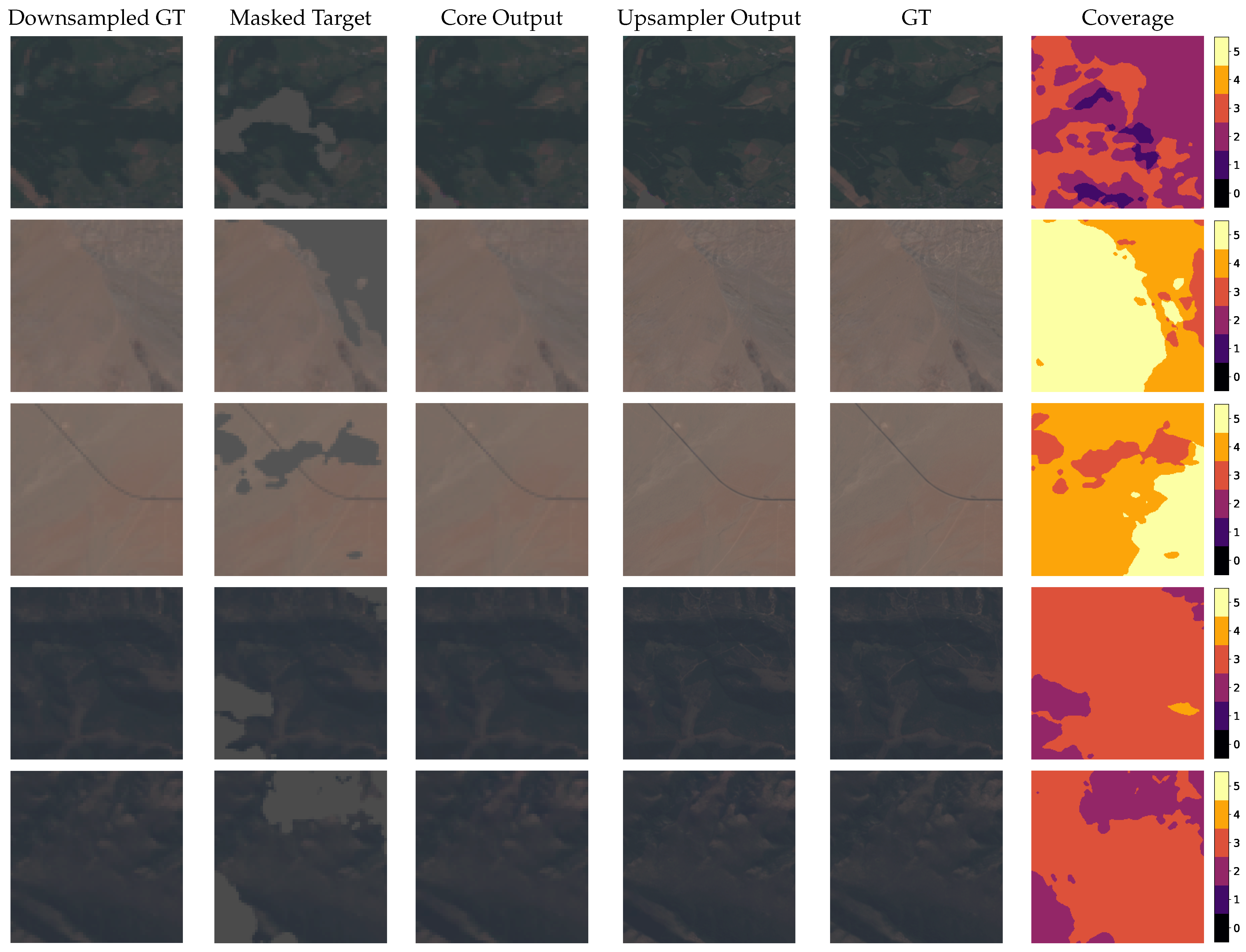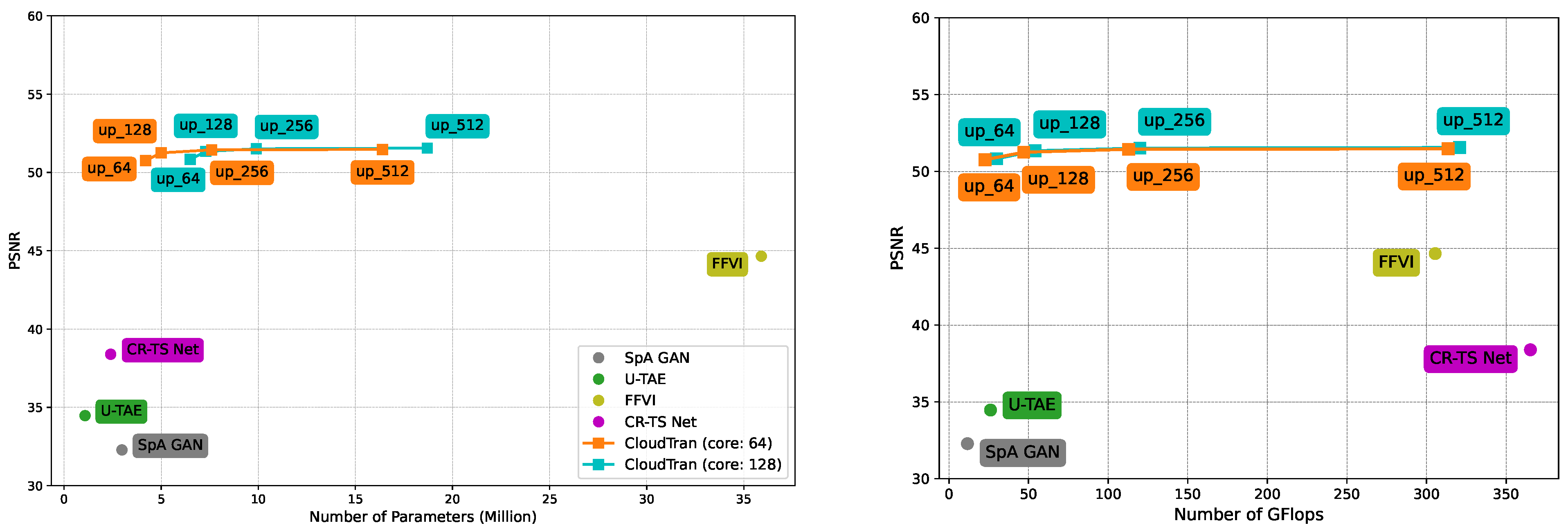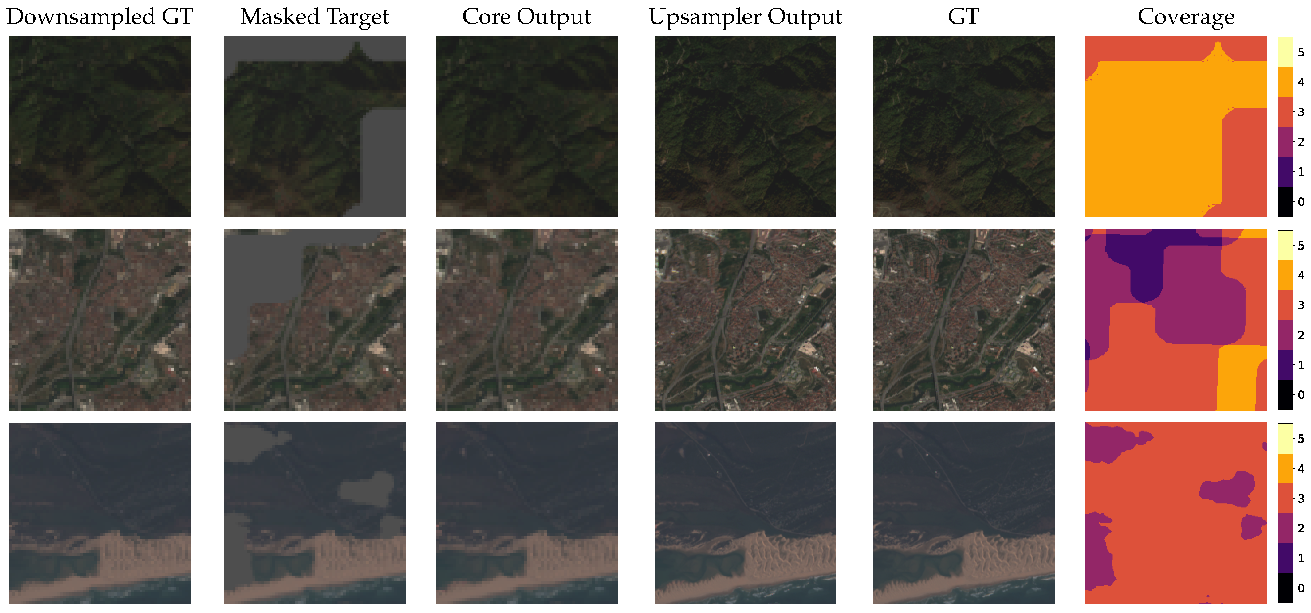To address this issue, following similar ideas from [31,32], we split the cloud removal problem into two sub-problems, each addressed by a specialized network. The first network (core) is an encoder-decoder model that performs cloud removal to a downsampled version of the original inputs, while the second one (upsampler) brings the output of the core network to the original resolution.

Specifically, the core network takes as input a stack of downsampled T image patches $I_t^{\downarrow }$, with $t\in \{1,2,\dots ,T\}$, and produces a cloud-free version of the downsampled target image $I_T^{\downarrow }$. The encoder, comprised of four layers of row and column attention, processes the input tensor ${\mathcal{H}}^{\downarrow }\in {\mathbf{R}}^{h\times w\times B\times T}$ made of T image patches corresponding to consecutive dates, with $h\times w$ the size of the downsampled images and B the number of bands considered. In each patch $I_t$, cloudy regions are masked out using image masks ${\mathcal{M}}^{\downarrow }$. Suitable embeddings are applied to the input, including positional encoding, which allows to explicitly model the non-uniform temporal differences between the images forming the tensor. Denoting d the embedding dimension, the encoder produces separate contexts ${\mathbf{c}}_t\in {\mathbf{R}}^{h\times w\times d}$ for each date which are subsequently aggregated, producing a single context $\overline{\mathbf{c}}\in {\mathbf{R}}^{h\times w\times d}$ for each band. The aggregated context $\overline{\mathbf{c}}$ is then used for conditioning the layers of the decoder whose output captures the per-pixel distribution over the admissible values of the downsampled cloud-free target image, conditioned on the input tensor ${\mathcal{H}}^{\downarrow }$, namely:

$${\displaystyle p_c\left(I_T^{\downarrow }\right|{\mathcal{H}}^{\downarrow })=\prod _i\prod _j{p}_c\left(I_T^{\downarrow }(i,j)|I_T^{\downarrow }(<i,·),I_T^{\downarrow }(i,<j),{\mathcal{H}}^{\downarrow }\right)}$$

(1)

The context is considered independently for each band $b\in B$ of the input tensor, and the model distinguishes between contexts corresponding to different bands via positional encoding.

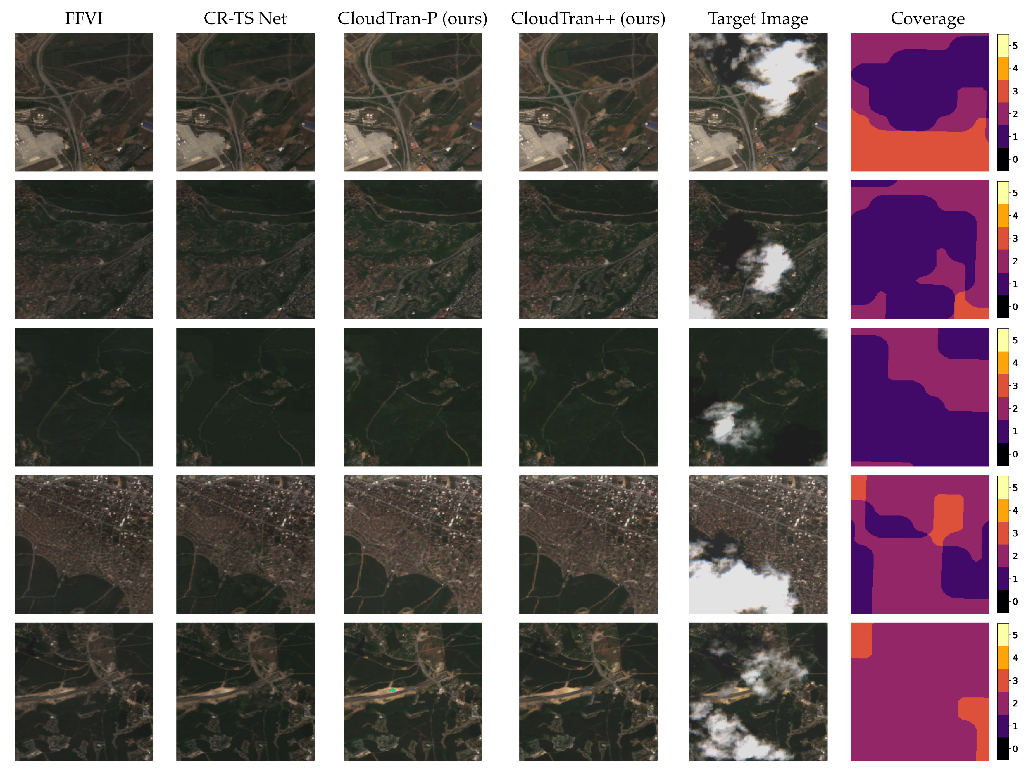
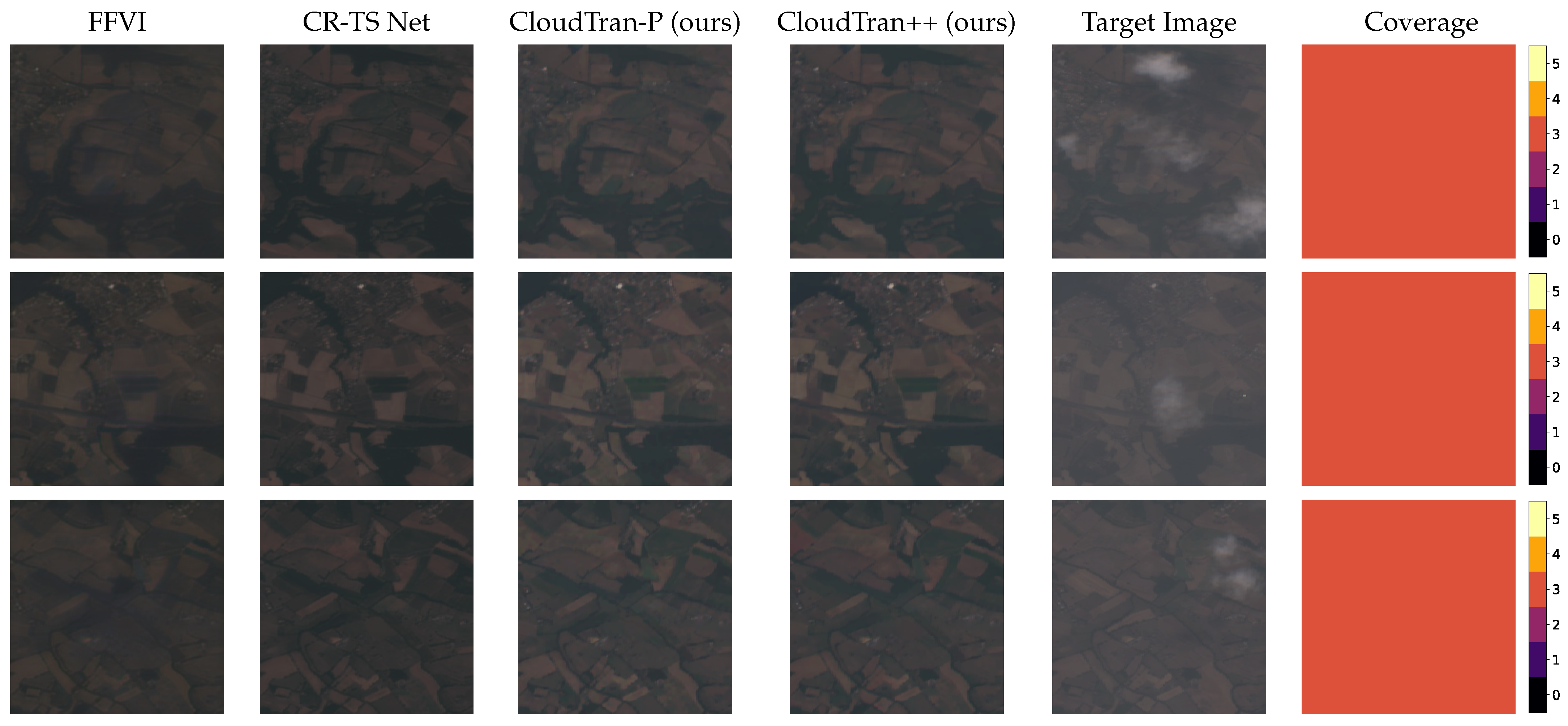
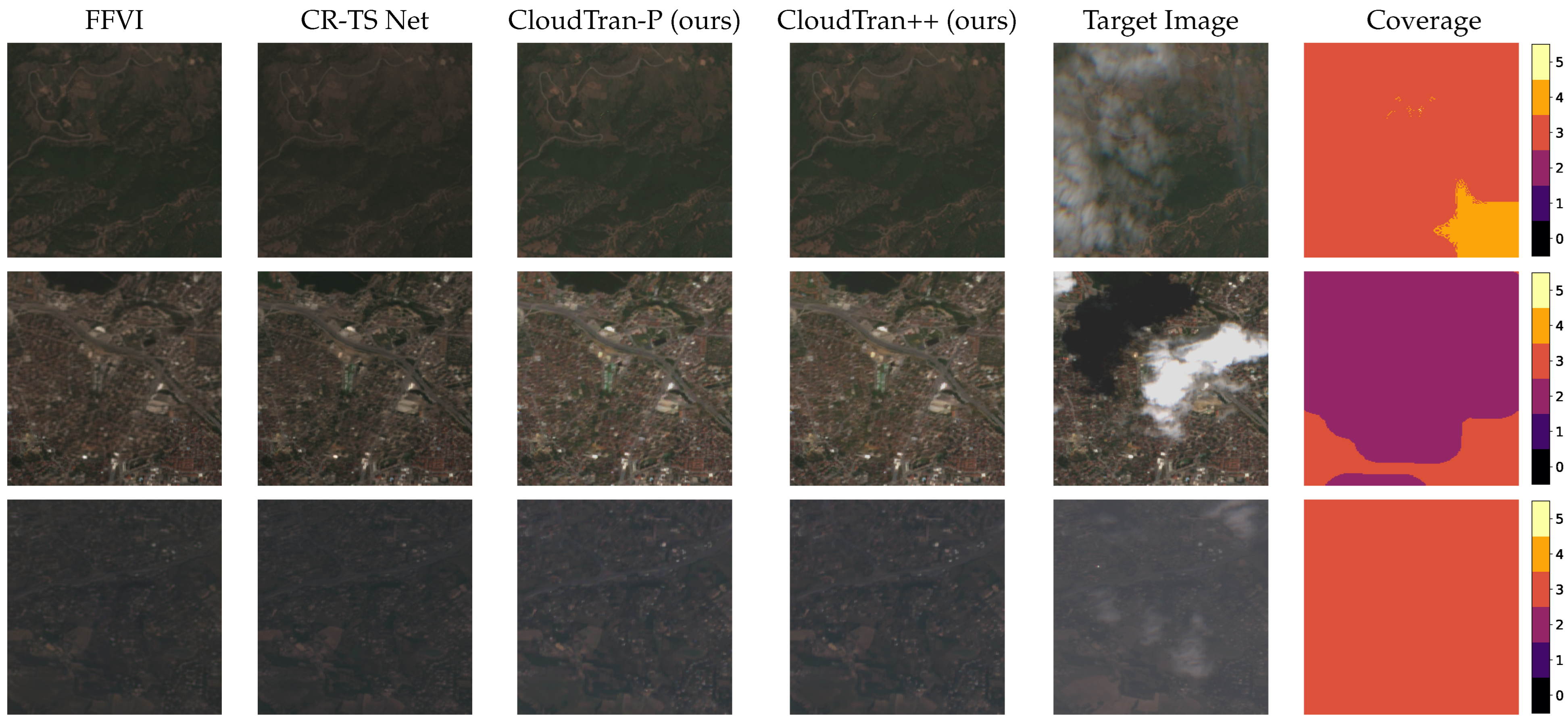
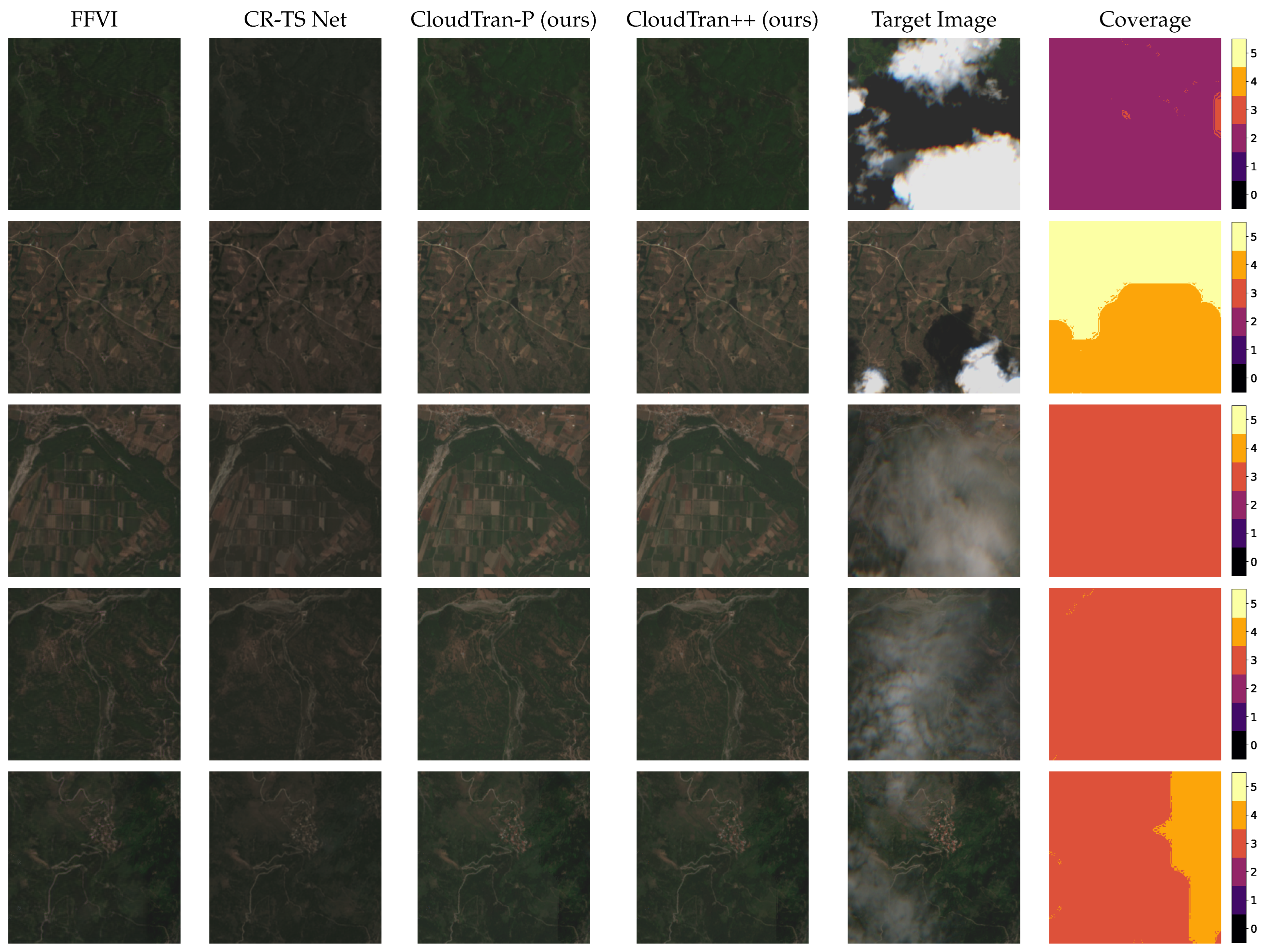
Similarly to [31], we also model the per-pixel distribution from the encoder output ${\tilde{p}}_c\left(I_T^{\downarrow }\right|{\mathcal{H}}^{\downarrow })$ to increase stability of the training process, by adding a dense and a softmax layer after the encoder’s aggregation layer. We denote this output of the model as CloudTran-Parallel (or in short, CloudTran-P), which due to its fully parallel nature is much more efficient for producing outputs in terms of time and computational cost, as in contrast to the full CloudTran++ model, it avoids autoregressive sampling (context recomputation for each pixel).

The upsampler network is a parallel model, i.e., all outputs are produced at once, given the input context. It is composed of three layers of row and column attention, and captures the per-pixel distribution of the cloud-free target image given the input tensor and the bilinearly upsampled cloud-free image, namely, $p_s\left(I_T\right|{\tilde{I}}_T^{\uparrow },\mathcal{H})$.

Each network is trained independently by minimizing the negative log-likelihood of the data, considering the cloud-free version of the last image $I_T^{GT}$, which, in the case of the core network, is also given as input to the decoder during training. During inference, to generate the low-resolution cloud-free image ${\tilde{I}}_T^{\downarrow }$, the context from the input data tensor is computed by the encoder given the input tensor ${\mathcal{H}}^{\downarrow }$. Based on the computed context, each pixel is sampled from the decoder in an autoregressive fashion, with previously sampled pixels being fed back to the decoder to condition generation of subsequent ones. We make use of the semi-parallel sampling property of axial transformers to speed up the sampling process, which avoids reevaluating the entire network for each pixel of the generated image. As the model considers the context corresponding to each band separately, sampling of each band is performed independently and the target image is obtained by stacking together the sampled bands. The image generated from the core network is then passed to the upsampler to produce the target cloud-free image ${\tilde{I}}_T$.

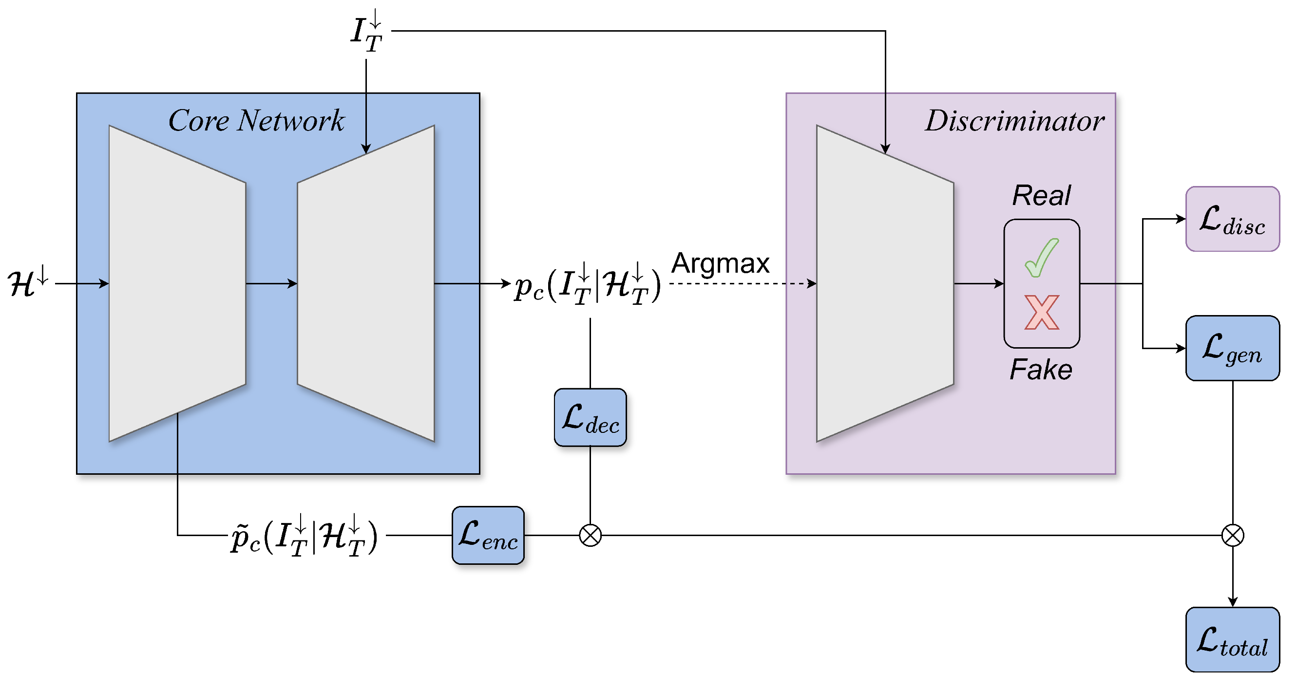
To limit the impact of the excessively bright values, we train a discriminator in parallel with our core network (Figure 2). The discriminator is a convolutional PatchGAN classifier as described in [33] and is responsible for the classification of an input image as real or fake. It has three inputs: the masked input image, the target ($I_T$) or the generated (${\tilde{I}}_T$) cloud-free image, and finally, the channel index of the corresponding training step. The first two inputs are concatenated together, resulting in a final output of a single band $30\times 30$ image patch. Inspired by WGAN [34], we incorporated a clip constraint, restricting the discriminator weights within a defined range, for enhanced training stability. We employ Binary Cross Entropy as the loss function for both the discriminator and the generator losses with a relative loss factor of $0.01$. The latter derives from the transformer output logits compared to discriminator outputs. Each discriminator model is optimized via Adam with a learning rate of $2\times {10}^{-4}$ and a momentum term $b_1=0.5$.

As a result, the total loss of our core network is given by Equation (2):

$${\mathcal{L}}_{total}={\lambda }_{dec}·{\mathcal{L}}_{dec}+{\lambda }_{enc}·{\mathcal{L}}_{enc}+{\lambda }_{gen}·{\mathcal{L}}_{gen}$$

(2)

where ${\mathcal{L}}_{dec}$, ${\mathcal{L}}_{enc}$ are the decoder and encoder loss functions that are based on the Cross entropy following a Softmax activation function, ${\mathcal{L}}_{gen}$ is the generator-like loss function for our transformer network, which serves as the generator in this context, based on the Binary Cross entropy, and ${\lambda }_{dec}$, ${\lambda }_{enc}$ and ${\lambda }_{gen}$ are the relative weighting factors for the encoder-decoder, encoder-only, and generator loss functions, respectively, with default values $0.99$, $0.01$ and $0.01$. Finally, we incorporate the Binary Cross entropy loss ${\mathcal{L}}_{disc}$ for the concurrent training of the discriminator network.

4. Experimental Evaluation

4.1. Datasets

4.1.1. In-House Multi-Temporal Dataset

We consider an in-house dataset consisting of fifty-six (56) Level-2A (L2A) products of Sentinel-2 satellite images, corresponding to different Days of Year (DOYs) in the period 2018–2019. Level-2A products provide Bottom of Atmosphere (BOA) reflectance images derived from the associated Level-1C products. Each product is a $109.8\times 109.8$ km² tile that extends across four regional units: Central Greece, Western Greece, Epirus and Thessaly. The dataset consists of ten (10) spectral bands with a wavelength range of 0.49–2.18 μm. We consider the bands B02, B03, B04 with 10 m spatial resolution and create multiband RGB tiles for each of the 56 different dates, from which we cut $512\times 512$ patches producing 441 multi-temporal patches of dimensions $512\times 512\times 3\times 56$ in total. The pixel values correspond to reflectances stored as 16-bit integers in the S2 product. As a final preprocessing step, the reflectances are divided with a fixed value for every band.

We compute cloud masks by considering all pixels with non-zero value in the CLD band that corresponds to each L2A product. We select a $5\times 5$ window of $512\times 512$ patches from every corner of the tile for testing/validation. This translates to a total of 100 regions ($\sim 20\%$) used for testing/validation, while the training set consists of the remaining 341 regions ($\sim 80\%$). In particular, the training set is defined by T consecutive image patches, with the last one corresponding to the summer period, so as to guarantee a cloud coverage below $5\%$. This is because the last image patch $I_T$ is used as a target.

4.1.2. SEN12MS-CR-TS (L1C Version)

We also consider the publicly available SEN12MS-CR-TS dataset [14] to further validate our proposed architecture. This multi-modal and multi-temporal dataset contains radar and optical observations collected via the Sentinel-1 and Sentinel-2 satellites for 53 ROIs (Regions Of Interest) worldwide (although only 43 were available in the published dataset at the time we accessed it), with 30 temporal samples provided for each patch-wise $256\times 256$ observation. In this work, we consider the bands B02, B03, B04 of Sentinel-2 images (Level 1C top-of-atmosphere reflectance products) to create 12,293 multi-temporal RGB patches in total. We follow the train/test splits indicated in [14], resulting in 1031 testing/validation and 11,262 training patches.

We produce cloud masks using the s2cloudless cloud detector [35], which takes as input the S2 image with its original 13 bands and returns the binary raster cloud mask, where 0 indicates pixels classified as clear-sky while 1 indicates pixels classified as clouds.

4.1.3. SEN12MS-CR-TS (L2A Version)

In order to validate the robustness of our network, we produce the Level-2A products corresponding to a subset of the SEN12MS-CR-TS dataset. This subset covers the regions of Europe and America with train/test splits as indicated in [14] (

Table 1. Number of (multi-temporal) patches for processed (Level-2A) version of SEN12MS-CR-TS covering Europe and America.

	Train	Test
America	1965	508
Europe	3930	1590
Total	5895	2098

).

To extract the Level-2A products from the respective Level-1C products, we employed the MAJA algorithm [36,37]. To match the specifications required by MAJA, we acquired, for every region of interest within the SEN12MS-CR-TS dataset across America and Europe, the raw Sentinel-2 Level-1C tiles. Consequently, we consider the B02, B03, B04 spectral bands, cropped according to a bounding box defined by the original patches of the Level-1C version of the dataset. This approach guarantees spatial correspondence between the two versions of the SEN12MS-CR-TS dataset, so they could be comparable.

Since calculating cloud masks on the fly limits our options in selecting the right cloud detection algorithm for the task, we utilize the CLD products derived from MAJA as pixel-based probabilities of cloud existence. Cloud shadows are also considered as non-valid pixels and, therefore, they are also masked out.

4.2. Implementation

We train the proposed CloudTran++ model on a Workstation equipped with two NVIDIA Quadro RTX 6000 GPUs with 24 GB of VRAM each. Unless explicitly stated otherwise, each model of the core transformer network has been trained for 50,000 iterations with a batch size equal to one, using the RMSProp algorithm with a learning rate equal to $3\times {10}^{-4}$, and by taking the exponential moving average of the parameters with a decay value equal to $0.999$. The same optimization parameters were used also for training the spatial upsampler.

The input tensor $\mathcal{H}$ is formed using patches corresponding to T consecutive dates, considering the last one $I_T$ as the target image. For the in-house dataset, the input patches are randomly cropped to $224\times 224$ for training and centrally cropped to the same dimension for evaluation. The SEN12MS-CR-TS dataset contains patches of $256\times 256$ and we define the input size for training and evaluation as $224\times 224$.

The inputs of the core model are first downsampled to $64\times 64$. During training, the clean target image $I_T$ is also provided as input to the decoder. For training the spatial upsampler, the target image is first downsampled and then bilinearly upsampled back to the original resolution, and fed to the model together with the input tensor $\mathcal{H}$. Supervision to both models is provided via the clean target image.

During inference, the input patches, masked with the corresponding cloud masks, are provided to the core model. The low-resolution cloud-free image is produced by sampling the model in an autoregressive fashion. This image is then provided to the spatial upsampler after bilinear upsampling, together with the input tensor $\mathcal{H}$. The pixel values of the cloud-free image are taken as the maximum likelihood estimates of the output distribution.

4.3. Evaluation Protocol

For training and validation, we consider T images from the training and testing validation split, respectively, captured during the summer period (DOY 55 for our dataset and 16 for SEN12MS-CR-TS L1C) to maximize the number of patches having a cloud-free target image, i.e., with a cloud coverage below $5\%$. For testing, we consider from within the testing/validation split, T dates in the spring period, and require that the target image has a cloud coverage above $5\%$.

Due to the extensive global coverage of both SEN12-MS-CR-TS datasets, a fixed reference index T defining the target image $I_T$ combined with the restriction that $I_T$ must exhibit cloud coverage below $5\%$, a large proportion of the initial time series patches are inevitably excluded during the training and validation phases. To address this issue within the SEN12MS-CR-TS L2A dataset and maximize the utilization of the available patches, we implement a flexible and adaptive approach in selecting the reference index. Thus, we investigated the optimal reference time index T for which the least cloudy $T-1$ consecutive patches were found. This approach was carried out in a geographical location (tile) scale, considering the inherent epoch diversity within the dataset.

During training, to mitigate the risk of overfitting and make our resulting model more robust, we consider an augmentation strategy by modifying randomly the contrast and brightness of each input tensor $\mathcal{H}$. The augmented dataset is subsequently concatenated and shuffled with the original dataset.

Regarding the cloud masks, for each dataset, we build a collection of masks with moderate coverage (typically, 5–30% coverage) $\mathcal{M}$, from all the patches of the corresponding dataset split. To increase the variety of masks that the models encounter during training, after masking out the clouds present in each patch, masks from $\mathcal{M}$ are randomly applied to each patch of the input tensor $\mathcal{H}$, before these are fed to the network. For validation, each patch is masked using the corresponding cloud mask, and a random mask from the collection is applied to the target image. For testing the networks in real cloud-covered patches, we consider tensors of T dates, where the last DOY, which corresponds to the reconstructed patch, is affected at least by moderate cloud coverage.

In terms of comparing our trained models with a strong multi-temporal cloud removal baseline, we implemented a ResNet-based architecture in a sequence-to-point style inspired by CR-TS Net [14]. The first part of the network consists of T Siamese ResNet branches responsible for cloud removal on each individual time point. Specifically, each ResNet branch consists of a 2D convolutional block followed by 16 sequential 2D ResNet blocks. The second part of the network aggregates the previous output feature maps in the temporal axis, feeding them into a 3D convolutional block and 5 sequential 3D ResNet blocks. The output of the network is a single cloud-free prediction, which is derived from a final 3D convolutional layer with a hyperbolic tangent (tanh()) activation function. As inputs, we consider the Sentinel-2 bands B02, B03, B04 with a temporal horizon $T=5$ and patch size $224\times 224$. Each model has been trained end-to-end for 50 epochs, and optimized via Adam with a learning rate of $2\times {10}^{-4}$ and a momentum term $b_1=0.5$. Due to the high number of GFlops occurring in the full network, we could only train these networks with a model size of 64. The masking strategy for training, validation and inference is identical to that described above for our models, where moderate cloud coverage was set to 5–30%.

4.4. Ablation

We perform several ablations on our dataset both for the core and the upsampler models to assess the contribution of different parameter choices on the quality of the reconstructed patches. The ablation results are compared with respect to the validation loss of the models, which is measured in bits per dimension (bits/dim) [38].

First, we study the effectiveness of the encoder’s context aggregation method used in the core network. The results are presented in

Table 2. Model performance in relation to the encoder’s context aggregation method in the core network. Symbol ↑ indicates higher is better and ↓ lower is better.

Context Aggregation	Validation Loss (↓)	PSNR (↑)	SSIM (↑)	MSE (↓)
Sum	1.4960	44.71	0.9810	3.976
Attention	0.3647	52.99	0.9969	0.957
Convolution	0.2674	54.48	0.9977	0.665

, where Sum corresponds to the depth-wise addition of the per-DOY contexts, Attention corresponds to the use of an attention block operating in the third axis of the context tensor, and Convolution corresponds to the use of $1\times 1$ convolution on the context tensor. It is evident that simple tensor reduction is not able to produce a single context summarizing sufficiently well the whole tensor. Learnable blocks on the other hand perform much better, reducing the validation loss by almost an order of magnitude. Between attention and convolution, the latter performs slightly better, while employing fewer parameters. Hence, unless otherwise stated, for the experiments that follow, we consider the $1\times 1$ convolution as the preferred context aggregation mechanism.

We also consider the impact of the model size on the final result. In particular,

Table 3. Model performance in relation to core model size. Symbol ↑ indicates higher is better and ↓ lower is better. Symbol # stands for number and NA stands for Not Available.

Model Size	Validation Loss (↓)	PSNR (↑)	SSIM (↑)	MSE (↓)	# Params
64	0.2898	52.76	0.9968	1.278	0.9 M
128	0.2782	52.88	0.9969	1.537	3.2 M
256	0.2674	54.48	0.9977	0.665	12.0 M
512	3.9090	NA	NA	NA	46.4 M

reports the validation loss for core models of size 64, 128, 256 and 512. The model size, defines the common size used for the input embedding, as well as the size of the attention block and the feed-forward block. Although, increasing the core model size from 64 to 128 and 256 improves the reconstruction quality, further increasing the model size to 512 leads to significant degradation. We justify this due to the large number of model parameters and the relatively small size of the dataset employed.

Table 4. Ablation on upsampler model size with core size 128 (baseline). Symbol ↑ indicates higher is better and ↓ lower is better. Symbol # stands for number.

Model Size	Validation Loss (↓)	PSNR (↑)	SSIM (↑)	MSE (↓)	# Params
64	0.3345	50.83	0.9961	1.289	0.5 M
128	0.3222	51.34	0.9963	1.200	1.3 M
256	0.3150	51.51	0.9963	1.167	3.9 M
512	0.3137	51.55	0.9964	1.149	12.7 M

and

Table 5. Ablation on upsampler model size with core size 64 (small). Symbol ↑ indicates higher is better and ↓ lower is better. Symbol # stands for number.

Model Size	Validation Loss (↓)	PSNR (↑)	SSIM (↑)	MSE (↓)	# Params
64	0.3345	50.76	0.9960	1.307	0.5 M
128	0.3222	51.25	0.9962	1.219	1.3 M
256	0.3150	51.44	0.9963	1.190	3.9 M
512	0.3137	51.47	0.9963	1.169	12.7 M

report the validation loss for spatial upsampler models of increasing size. Table 4 showcases results obtained with a core model of size 128, while Table 5 refers to a core model size 64. We can see here, that in both cases, increasing the model size leads to higher reconstruction quality. Nevertheless, as this model also operates to much larger inputs, and considering that the complexity is $\mathcal{O}\left(n\sqrt{n}\right)$, increasing the model size leads to significant increase in memory footprint. Due to this, 512 is the largest model size we could afford.

We also consider the effect of the number of DOYs T forming the input tensor and the percentage of cloud coverage considered of the masks employed during training. The respective results are shown in Figure 3. We observe that training with three DOYs leads to a higher validation loss compared to five DOYs. This outcome is expected, as fewer temporal contexts (smaller number of DOYs) provide limited information, making cloud removal less effective. The higher validation loss observed for four DOYs can most likely be attributed to errors introduced by adding noisy cloudy images without valuable temporal context. Increasing the number of DOYs to five or more stabilizes the training process, improving robustness and generalization. Regarding cloud coverage, we observe that when masks with higher coverage are used during training, the validation loss initially decreases and then remains, to a large extent, constant. This is reasonable as the model becomes more robust in reconstructing larger areas affected by clouds. Nevertheless, the differences in validation loss are small, showing that the proposed method is quite robust both with respect to the number of DOYs and the amount of mask cloud coverage employed during training.

Finally,

Table 6. Ablation on augmentation techniques and discriminator. Symbol ↑ indicates higher is better and ↓ lower is better. Symbol ✓ represents use of corresponding feature and ✗ its absence.

Augmentation	Discriminator	Validation Loss (↓)	PSNR (↑)	SSIM (↑)	MSE (↓)
✗	✗	0.2674	54.48	0.9977	0.665
✗	✓	0.2682	54.14	0.9975	0.803
✓	✗	0.2823	53.70	0.9970	0.901
✓	✓	0.2711	54.32	0.9975	0.709

reviews the utilization of the discriminator network and the augmentation techniques considered in this paper. We can see that using the discriminator network during training and augmentation methods together outperforms the models trained considering each of these features alone. On the other hand, the model that uses none of those features, leads to better metrics on this particular dataset; however, it is less adaptive to domain changes and more challenging datasets. Specifically, the in-house dataset features limited variations as it concerns a specific geographic region, enabling even simpler versions of the model to learn and generalize. In contrast, when evaluated on more complex datasets, such as SEN12MS-CR-TS that covers a wide variaty of geographic regions, we observed that incorporating both the discriminator network and augmentation techniques consistently improve the model’s generalization ability.

4.5. Quantitative and Qualitative Results

Based on the ablation study, we consider in this section a core model of size 128 reconstructing the reduced resolution target image ($64\times 64$), followed by an upsampler model of size 512, that together produce the cloud-less target image in full resolution. We perform quantitative evaluation considering the Mean Squared Error (MSE), Peak Signal-to-Noise Ratio (PSNR) and Structural Similarity (SSIM) metrics with respect to the validation set of each dataset [39]. Additionally, we calculate the Fréchet Inception Distance (FID) [40] and the Kernel Inception Distance (KID) [41].

Table 7. Comparison with multi-temporal cloud removal methods on in-house dataset for $64\times 64$ outputs. Symbol ↑ indicates higher is better and ↓ lower is better. CloudTran-P indicates the CloudTran++ parallel model. Symbol # stands for number and NA stands for Not Available. Tran. stands for Transformer network and Disc. for discriminator. Best results are in bold.

Method	PSNR (↑)	SSIM (↑)	MSE (↓)	# Params
SpA GAN [9]	33.55	0.9310	46.982	2.98 M
Median	32.89	0.8540	55.720	NA
FFVI [28]	44.61	0.9796	2.977	35.9 M
U-TAE [42]	36.46	0.9117	27.470	1.08 M
CloudTran-P (core: 64)	51.69	0.9957	1.213	0.9 M Tran. + 2.8 M Disc. = 3.7 M
CloudTran++ (core: 64)	53.34	0.9969	0.914
CloudTran-P (baseline)	51.83	0.9958	1.193	3.2 M Tran. + 2.8 M Disc. = 6 M
CloudTran++ (baseline)	53.75	0.9971	0.880

and

Table 8. Comparison with multi-temporal cloud removal methods on in-house dataset for $224\times 224$ outputs. Symbol ↑ indicates higher is better and ↓ lower is better. CloudTran-P indicates the CloudTran++ parallel model. Symbol # stands for number and NA stands for Not Available. C and Up in the last column indicate the Core and Upsampler networks, respectively. Best results are in bold.

Method	PSNR (↑)	SSIM (↑)	MSE (↓)	# Params
SpA GAN [9]	32.28	0.9144	58.323	2.98 M
Median	30.94	0.8335	87.30	NA
FFVI [28]	44.65	0.9833	3.106	35.9 M
U-TAE [42]	34.47	0.8697	31.802	1.08 M
CR-TS Net [14]	38.39	0.9404	10.341	2.4 M
CloudTran-P (core: 64)	50.42	0.9956	1.435	3.7 M C + 0.5 M Up = 4.2 M
CloudTran++ (core: 64)	50.76	0.9960	1.307
CloudTran-P (baseline)	50.95	0.9958	1.339	6 M C + 12.7 M Up = 18.7 M
CloudTran++ (baseline)	51.55	0.9964	1.149

compare the performance of the proposed CloudTran++ method with different baselines for the low- and full-resolution outputs, respectively. In particular, we consider a suitably adapted version of the powerful video inpainting method of [28], as well as a standard gap-filling method based on rolling median filtering and CR-TS Net, a 3D-ResNet sequence-to-point model by [14], discussed in detail above. Table 7, considers only the core model, while Table 8 reports the results using the entire architecture. We also report the performance of the method proposed by [9] based on SpA GAN, as an indicative case of single-image cloud removal methods, utilizing Generative Adversarial Networks. SpA GAN employs a single temporal instance, justifying the relatively high MSE values. Finally, we adapt the U-TAE architecture [42], which was initially designed for panoptic and semantic segmentation on satellite time-series, to perform cloud removal. U-TAE introduced a method for spatio-temporal encoding, with a shared convolutional encoder across the temporal axis. In our adaptation, instead of generating segmentation maps, the output of the U-TAE decoder is used to reconstruct cloud-free RGB images to address the cloud removal task. We trained this repurposed architecture for 200 epochs using the Mean Squared Error (MSE) loss to optimize reconstruction accuracy.

Our models outperform the baselines with a significant margin both for reduced- and full-resolution results, while using fewer trainable parameters than the second-best FFVI. Although the CR-TS Net model with size 64 has fewer trainable parameters, it requires a considerably large amount of GFlops (Figure 4).

Both tables also report the results obtained using solely the encoder output as CloudTran Parallel. Being a parallel model, its sampling is much more efficient, but the quality of the model produced is inferior as the samples are more affected by artifacts.

Nevertheless, it still performs better than other baselines.

Table 9. Comparison of cloud removal methods for $224\times 224$ outputs of SEN12MS-CR-TS dataset. Average metrics on the entire dataset are reported. Symbol ↑ indicates higher is better and ↓ lower is better. CloudTran-P indicates the CloudTran++ parallel model. Best values are shown in bold and second-best values are underlined.

Method	L1C Version					L2A Version
	PSNR (↑)	SSIM (↑)	MSE (↓)	FID (↓)	KID (↓) ($\mathbf{\times }{\mathbf{10}}^{\mathbf{-}\mathbf{3}}$)	PSNR (↑)	SSIM (↑)	MSE (↓)	FID (↓)	KID (↓) ($\mathbf{\times }{\mathbf{10}}^{\mathbf{-}\mathbf{3}}$)
SpA GAN [9]	28.76	0.8847	131.22	4.529	$1.93\pm 0.16$	23.31	0.5716	442.08	4.170	$\mathbf{1.73}\pm \mathbf{0.13}$
Median	26.18	0.8017	274.66	4.855	$1.89\pm 0.16$	27.47	0.7651	249.72	4.081	$1.93\pm 0.18$
FFVI [28]	51.17	0.9948	1.292	4.808	$1.87\pm 0.14$	40.77	0.9731	10.383	4.033	$1.90\pm 0.16$
U-TAE [42]	23.26	0.7989	4914.2	4.388	$2.06\pm 0.15$	29.46	0.8244	128.26	3.840	$1.88\pm 0.17$
CR-TS Net [14]	39.55	0.9848	8.327	4.274	$1.89\pm 0.17$	35.93	0.8839	20.510	4.285	$2.15\pm 0.22$
CloudTran-P	46.62	0.9890	8.758	4.263	$1.76\pm 0.18$	39.83	0.9691	16.790	4.317	$2.05\pm 0.22$
CloudTran++	52.83	0.9957	1.957	4.156	$\mathbf{1.75}\pm \mathbf{0.15}$	41.27	0.9750	13.163	3.949	$1.88\pm 0.19$

also reports the results of median filtering, SpA-GAN, FFVI, U-TAE, CR-TS Net and CloudTran++, on both versions of the SEN12MS-CR-TS dataset. Our models have been trained on the SEN12MS-CR-TS dataset for 200,000 iterations in either case. Our full model achieves PSNR values of $52.83/41.27$ dB, SSIM values of $0.9957/0.9750$ and MSE equal to $1.957/13.163$ on the validation set of the L1C and L2A versions, respectively. These values are not directly comparable to the ones reported in [14] for numerous reasons. Just to mention some of them, [14] considers also data from Sentinel 1, processing is performed in a sequence-to-sequence fashion, and also validation is defined differently. Nevertheless, the values reported on the SEN12MS-CR-TS dataset are significantly improved with respect to the ones reported in [14] and the ones obtained by a fully trained CR-TS Net model of size 64.

The FID/KID metrics were calculated using a ResNet50 feature extractor, pretrained on the RGB version of the SSL4EO-S12 dataset [43]. The reported values are based on the difference between the extracted ResNet50 features of the EuroSAT dataset (Sentinel-2, Level-1C imagery) [44] and the respective features of the cloud-free generated images. Table 9 shows that the CloudTran++ and CloudTran parallel models achieve lower FID/KID values than the CR-TS Net on sample outputs from both the L1C and L2A versions of SEN12-MS-CR-TS.

Figure 5 shows randomly chosen cloud removal results obtained by our models on the validation set of the three datasets. The first column shows the downsampled ground truth target image, the second shows the target image after applying the cloud mask, and the third one shows the cloud-free image produced by the core model. The next two columns show the output of the upsampler and the ground truth image in the original resolution. The last column shows for each location the number of cloud-free pixels in the input tensor.

Figure 6 shows randomly chosen results from the test sets of the three datasets considered. Here, the first two columns show the results of the FFVI [28] and the sequence-to-point CR-TS Net model based on [14]. The third and fourth columns show the results of the proposed CloudTran++ model from the encoder and the decoder, respectively. The original unmasked image and the cloud coverage are shown in the last two columns. We observe that the results of the proposed method contain fewer artifacts and are more faithful to the corresponding inputs. More validation and test results for each dataset can be found in the Appendix A.

Finally, Figure 7 presents some failure cases caused by different contributing factors. To mention some of them, time-series affected by severe (>50%) cloud coverage in all but 1 or 2 patches forming the input tensor may lead to failures. Additionally, vast sea regions of interest and patches representing seasonal changes, such as crop fields, within the input tensor $\mathcal{H}$, prove to be more challenging to predict.

5. Conclusions

Our work introduces a cloud-removal architecture based on two transformer-based models using axial attention blocks for increased efficiency. An encoder-decoder model is proposed for producing low-resolution cloud-free images in an autoregressive fashion, given a number of input patches where the cloudy regions have been masked-out. A parallel output based only on the encoder of the core network is utilized to reduce sampling time and increase training stability. An encoder-only parallel model is proposed for upsampling the cloud-free image to the original resolution. The proposed model is shown to perform significantly better with respect to a number of strong baselines, across different sentinel-2 datasets. Finally, by making publicly available the three datasets considered in this work, we aim to facilitate further advancements in the field of multi-temporal remote sensing tasks.

References

1. Liu, S.; Marinelli, D.; Bruzzone, L.; Bovolo, F. A review of change detection in multitemporal hyperspectral images: Current techniques, applications, and challenges. IEEE Geosci. Remote Sens. Mag. 2019, 7, 140–158. [Google Scholar] [CrossRef]
2. Papadomanolaki, M.; Vakalopoulou, M.; Karantzalos, K. A Deep Multitask Learning Framework Coupling Semantic Segmentation and Fully Convolutional LSTM Networks for Urban Change Detection. IEEE Trans. Geosci. Remote Sens. 2021, 59, 7651–7668. [Google Scholar] [CrossRef]
3. Karakizi, C.; Karantzalos, K.; Vakalopoulou, M.; Antoniou, G. Detailed land cover mapping from multitemporal landsat-8 data of different cloud cover. Remote Sens. 2018, 10, 1214. [Google Scholar] [CrossRef]
4. Franchetti, B.; Ntouskos, V.; Giuliani, P.; Herman, T.; Barnes, L.; Pirri, F. Vision Based Modeling of Plants Phenotyping in Vertical Farming under Artificial Lighting. Sensors 2019, 19, 4378. [Google Scholar] [CrossRef]
5. Schmitt, M.; Prexl, J.; Ebel, P.; Liebel, L.; Zhu, X.X. Weakly Supervised Semantic Segmentation of Satellite Images for Land Cover Mapping—Challenges and Opportunities. arXiv 2020, arXiv:2002.08254. [Google Scholar] [CrossRef]
6. Ding, L.; Lin, D.; Lin, S.; Zhang, J.; Cui, X.; Wang, Y.; Tang, H.; Bruzzone, L. Looking Outside the Window: Wide-Context Transformer for the Semantic Segmentation of High-Resolution Remote Sensing Images. IEEE Trans. Geosci. Remote Sens. 2022, 60, 4410313. [Google Scholar] [CrossRef]
7. Tang, X.; Ma, Q.; Zhang, X.; Liu, F.; Ma, J.; Jiao, L. Attention Consistent Network for Remote Sensing Scene Classification. IEEE J. Sel. Top. Appl. Earth Obs. Remote Sens. 2021, 14, 2030–2045. [Google Scholar] [CrossRef]
8. Singh, P.; Komodakis, N. Cloud-gan: Cloud removal for sentinel-2 imagery using a cyclic consistent generative adversarial networks. In Proceedings of the IEEE International Geoscience and Remote Sensing Symposium, Valencia, Spain, 22–27 July 2018; pp. 1772–1775. [Google Scholar]
9. Pan, H. Cloud Removal for Remote Sensing Imagery via Spatial Attention Generative Adversarial Network. arXiv 2020, arXiv:2009.13015. [Google Scholar]
10. Wu, P.; Pan, Z.; Tang, H.; Hu, Y. Cloudformer: A Cloud-Removal Network Combining Self-Attention Mechanism and Convolution. Remote Sens. 2022, 14, 6132. [Google Scholar] [CrossRef]
11. Ma, X.; Huang, Y.; Zhang, X.; Pun, M.O.; Huang, B. Cloud-EGAN: Rethinking CycleGAN From a Feature Enhancement Perspective for Cloud Removal by Combining CNN and Transformer. IEEE J. Sel. Top. Appl. Earth Obs. Remote Sens. 2023, 16, 4999–5012. [Google Scholar] [CrossRef]
12. Sarukkai, V.; Jain, A.; Uzkent, B.; Ermon, S. Cloud Removal from Satellite Images using Spatiotemporal Generator Networks. In Proceedings of the IEEE/CVF Winter Conference on Applications of Computer Vision (WACV), Snowmass, CO, USA, 1–5 March 2020. [Google Scholar]
13. Boston, T.; Van Dijk, A.; Thackway, R. Convolutional Neural Network Shows Greater Spatial and Temporal Stability in Multi-Annual Land Cover Mapping Than Pixel-Based Methods. Remote Sens. 2023, 15, 2132. [Google Scholar] [CrossRef]
14. Ebel, P.; Xu, Y.; Schmitt, M.; Zhu, X.X. SEN12MS-CR-TS: A Remote Sensing Data Set for Multi-modal Multi-temporal Cloud Removal. IEEE Trans. Geosci. Remote Sens. 2022, 60. [Google Scholar] [CrossRef]
15. Sebastianelli, A.; Puglisi, E.; Del Rosso, M.P.; Mifdal, J.; Nowakowski, A.; Mathieu, P.P.; Pirri, F.; Ullo, S.L. PLFM: Pixel-Level Merging of Intermediate Feature Maps by Disentangling and Fusing Spatial and Temporal Data for Cloud Removal. IEEE Trans. Geosci. Remote Sens. 2022, 60, 5412216. [Google Scholar] [CrossRef]
16. Zhao, X.; Jia, K. Cloud Removal in Remote Sensing Using Sequential-Based Diffusion Models. Remote Sens. 2023, 15, 2861. [Google Scholar] [CrossRef]
17. Vaswani, A.; Shazeer, N.; Parmar, N.; Uszkoreit, J.; Jones, L.; Gomez, A.N.; Kaiser, Ł.; Polosukhin, I. Attention is all you need. In Proceedings of the Advances in Neural Information Processing Systems, Long Beach, CA, USA, 4–9 December 2017; pp. 5998–6008. [Google Scholar]
18. Dosovitskiy, A.; Beyer, L.; Kolesnikov, A.; Weissenborn, D.; Zhai, X.; Unterthiner, T.; Dehghani, M.; Minderer, M.; Heigold, G.; Gelly, S.; et al. An image is worth 16x16 words: Transformers for image recognition at scale. arXiv 2020, arXiv:2010.11929. [Google Scholar]
19. He, K.; Chen, X.; Xie, S.; Li, Y.; Doll’ar, P.; Girshick, R.B. Masked Autoencoders Are Scalable Vision Learners. In Proceedings of the 2022 IEEE/CVF Conference on Computer Vision and Pattern Recognition (CVPR), New Orleans, LA, USA, 18–24 June 2022; pp. 15979–15988. [Google Scholar]
20. Bazi, Y.; Bashmal, L.; Rahhal, M.M.A.; Dayil, R.A.; Ajlan, N.A. Vision transformers for remote sensing image classification. Remote Sens. 2021, 13, 516. [Google Scholar] [CrossRef]
21. Zhang, J.; Zhao, H.; Li, J. TRS: Transformers for Remote Sensing Scene Classification. Remote. Sens. 2021, 13, 4143. [Google Scholar] [CrossRef]
22. Ho, J.; Kalchbrenner, N.; Weissenborn, D.; Salimans, T. Axial attention in multidimensional transformers. arXiv 2019, arXiv:1912.12180. [Google Scholar]
23. Christopoulos, D.; Ntouskos, V.; Karantzalos, K. Cloudtran: Cloud Removal from Multitemporal Satellite Images Using Axial Transformer Networks. Int. Arch. Photogramm. Remote Sens. Spat. Inf. Sci. 2022, 43, 1125–1132. [Google Scholar] [CrossRef]
24. Liu, L.; Hu, S. SACTNet: Spatial Attention Context Transformation Network for Cloud Removal. Wirel. Commun. Mob. Comput. 2021, 2021, 8292612. [Google Scholar] [CrossRef]
25. Lin, C.H.; Tsai, P.H.; Lai, K.H.; Chen, J.Y. Cloud removal from multitemporal satellite images using information cloning. IEEE Trans. Geosci. Remote Sens. 2012, 51, 232–241. [Google Scholar] [CrossRef]
26. Ebel, P.; Garnot, V.S.F.; Schmitt, M.; Wegner, J.D.; Zhu, X.X. UnCRtainTS: Uncertainty Quantification for Cloud Removal in Optical Satellite Time Series. In Proceedings of the IEEE/CVF Conference on Computer Vision and Pattern Recognition (CVPR) Workshops, Vancouver, BC, Canada, 17–24 June 2023; pp. 2086–2096. [Google Scholar]
27. Liu, W.; Cui, H.; Jiang, Y.; Zhang, G.; Li, X.; Li, H.; Chen, Y.; Yang, J. DecRecNet: A Decoupling-Reconstruction Network for Restoring the Missing Information of Optical Remote Sensing Images. IEEE J. Sel. Top. Appl. Earth Obs. Remote Sens. 2023, 16, 9777–9801. [Google Scholar] [CrossRef]
28. Chang, Y.L.; Liu, Z.Y.; Lee, K.Y.; Hsu, W. Free-form video inpainting with 3D gated convolution and temporal PatchGAN. In Proceedings of the IEEE International Conference on Computer Vision, Seoul, Republic of Korea, 27–28 October 2019; pp. 9066–9075. [Google Scholar]
29. Liu, R.; Deng, H.; Huang, Y.; Shi, X.; Lu, L.; Sun, W.; Wang, X.; Dai, J.; Li, H. Fuseformer: Fusing fine-grained information in transformers for video inpainting. In Proceedings of the IEEE International Conference on Computer Vision, Montreal, BC, Canada, 11–17 October 2021; pp. 14040–14049. [Google Scholar]
30. Khan, S.; Naseer, M.; Hayat, M.; Zamir, S.W.; Khan, F.S.; Shah, M. Transformers in Vision: A Survey. ACM Comput. Surv. 2022, 54, 1–41. [Google Scholar] [CrossRef]
31. Kumar, M.; Weissenborn, D.; Kalchbrenner, N. Colorization Transformer. In Proceedings of the International Conference on Learning Representations, Vienna, Austria, 4 May 2021. [Google Scholar]
32. Menick, J.; Kalchbrenner, N. Generating high fidelity images with subscale pixel networks and multidimensional upscaling. In Proceedings of the International Conference on Learning Representations, New Orleans, LA, USA, 6–9 May 2019. [Google Scholar]
33. Isola, P.; Zhu, J.Y.; Zhou, T.; Efros, A.A. Image-to-Image Translation with Conditional Adversarial Networks. arXiv 2018, arXiv:1611.07004. [Google Scholar]
34. Arjovsky, M.; Chintala, S.; Bottou, L. Wasserstein GAN. arXiv 2017, arXiv:1701.07875. [Google Scholar]
35. Skakun, S.; Wevers, J.; Brockmann, C.; Doxani, G.; Aleksandrov, M.; Batič, M.; Frantz, D.; Gascon, F.; Gómez-Chova, L.; Hagolle, O.; et al. Cloud Mask Intercomparison eXercise (CMIX): An evaluation of cloud masking algorithms for Landsat 8 and Sentinel-2. Remote Sens. Environ. 2022, 274, 112990. [Google Scholar] [CrossRef]
36. Hagolle, O.; Huc, M.; Pascual, D.V.; Dedieu, G. A multi-temporal method for cloud detection, applied to FORMOSAT-2, VENµS, LANDSAT and SENTINEL-2 images. Remote Sens. Environ. 2010, 114, 1747–1755. [Google Scholar] [CrossRef]
37. Hagolle, O.; Huc, M.; Desjardins, C.; Auer, S.; Richter, R. MAJA Algorithm Theoretical Basis Document. 2018. Available online: https://zenodo.org/records/1209633 (accessed on 21 February 2023). [CrossRef]
38. Papamakarios, G.; Pavlakou, T.; Murray, I. Masked autoregressive flow for density estimation. In Proceedings of the Advances in Neural Information Processing Systems, Long Beach, CA, USA, 4–9 December 2017; Volume 30. [Google Scholar]
39. Wang, Z.; Bovik, A.C.; Sheikh, H.R.; Simoncelli, E.P. Image quality assessment: From error visibility to structural similarity. IEEE Trans. Image Process. 2004, 13, 600–612. [Google Scholar] [CrossRef]
40. Heusel, M.; Ramsauer, H.; Unterthiner, T.; Nessler, B.; Klambauer, G.; Hochreiter, S. GANs Trained by a Two Time-Scale Update Rule Converge to a Nash Equilibrium. arXiv 2017, arXiv:1706.08500. [Google Scholar]
41. Bińkowski, M.; Sutherland, D.J.; Arbel, M.; Gretton, A. Demystifying MMD GANs. arXiv 2021, arXiv:1801.01401. [Google Scholar]
42. Garnot, V.S.F.; Landrieu, L. Panoptic Segmentation of Satellite Image Time Series with Convolutional Temporal Attention Networks. In Proceedings of the 2021 IEEE/CVF International Conference on Computer Vision, ICCV 2021, Montreal, QC, Canada, 10–17 October 2021; pp. 4852–4861. [Google Scholar] [CrossRef]
43. Wang, Y.; Braham, N.A.A.; Xiong, Z.; Liu, C.; Albrecht, C.M.; Zhu, X.X. SSL4EO-S12: A Large-Scale Multi-Modal, Multi-Temporal Dataset for Self-Supervised Learning in Earth Observation. arXiv 2023, arXiv:2211.07044. [Google Scholar]
44. Helber, P.; Bischke, B.; Dengel, A.; Borth, D. Eurosat: A novel dataset and deep learning benchmark for land use and land cover classification. IEEE J. Sel. Top. Appl. Earth Obs. Remote Sens. 2019, 12, 2217–2226. [Google Scholar] [CrossRef]
Figure 1. CloudTran architecture: The core network takes as input T reduced-resolution images where clouds are masked and generates the cloud-free image corresponding to the last date. An upsampler network is used to generate the full-resolution cloud-free image based on the core network output, conditioned on the T original masked images. The symbol ⊗ indicates summation of ingoing quantities.
Remotesensing 17 00086 g001
Figure 2. Addition of discriminator during the core network training for addressing outlying values in the generated images. The symbol ⊗ indicates summation of ingoing quantities.
Remotesensing 17 00086 g002
Figure 3. Validation loss in relation to number of DOYs provided as input and maximum cloud coverage considered during training. Symbol # stands for number.
Remotesensing 17 00086 g003
Figure 4. Model comparison with respect to the total number of parameters.
Remotesensing 17 00086 g004
Figure 5. Cloud-free images generated using the proposed method randomly selected from the validation set of the three datasets considered. First row: in-house dataset, 2nd row: processed (Level-2A) SEN12MS-CR-TS dataset of Europe and America, 3rd row: original SEN12MS-CR-TS (Level-1C) dataset. (Best viewed on screen zoomed-in).
Remotesensing 17 00086 g005
Figure 6. Comparison of cloud-free images generated using the proposed method with multi-temporal cloud removal methods for randomly selected patches taken from the test set of the three datasets considered. First row: in-house dataset, 2nd row: processed (Level-2A) SEN12MS-CR-TS dataset of Europe and America, 3rd row: original SEN12MS-CR-TS (Level-1C) dataset. FFVI is based on [28] and 3D-ResNet on [14]. CloudTran-P results are based solely on the encoder output of the core-network. (Best viewed on screen zoomed-in).
Remotesensing 17 00086 g006
Figure 7. Failure cases (top) and corresponding ground truth images (bottom).
Remotesensing 17 00086 g007