
Deep Learning Applications in Ionospheric Modeling: Progress, Challenges, and Opportunities

 ,
,  ,
,  and
and 
Abstract
:1. Introduction
2. Data Challenges in Ionospheric Modeling
2.1. Primary Data Sources
2.2. Data Preprocessing Algorithms
3. Progress of Ionospheric Modeling Based on Deep Learning Technology
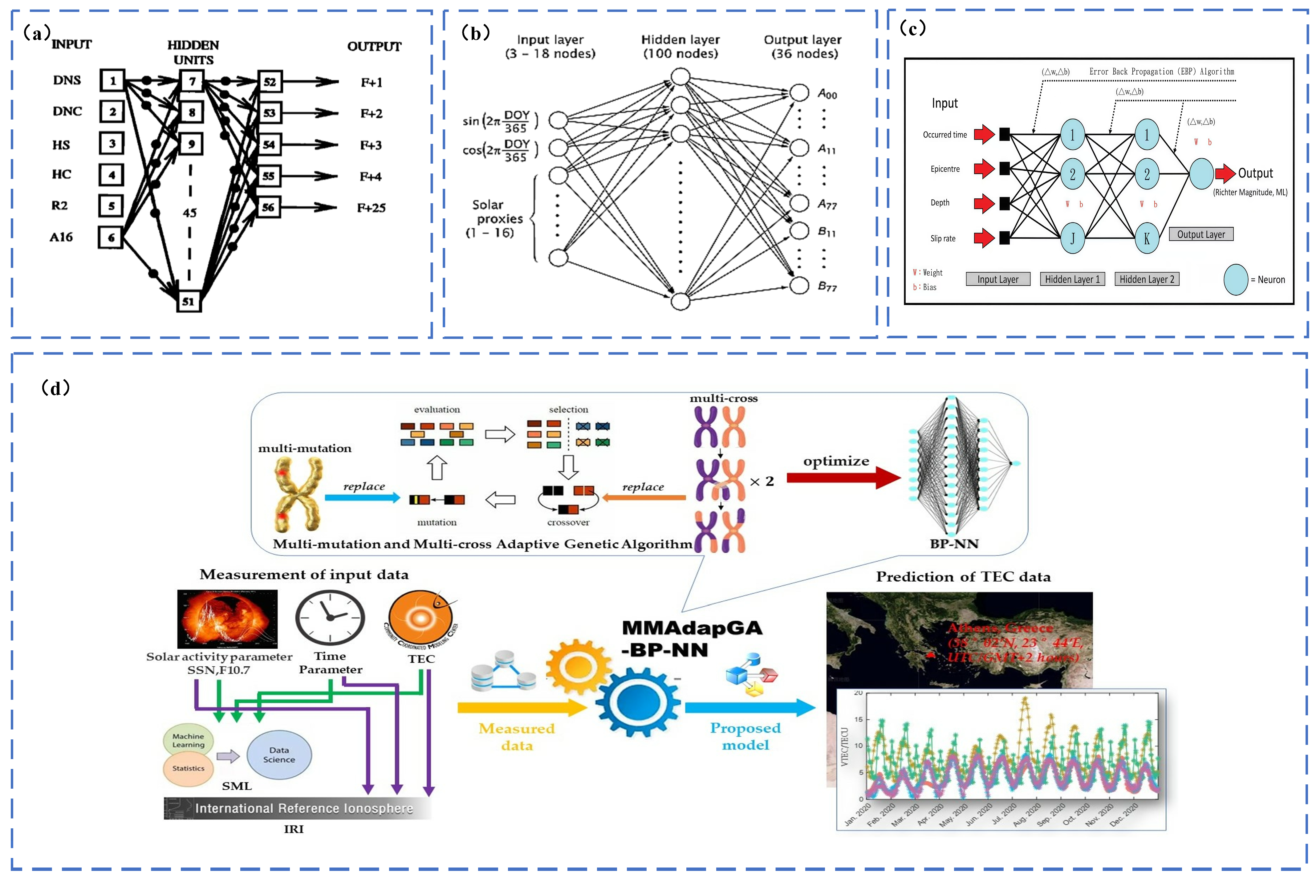
3.1. Backpropagation (BP) Neural Network

| Source | Method | Main Features and Results |
|---|---|---|
| Weng et al. [52] | MMAdapGA-BP-NN |
|
| Lei et al. [88] | GA-BP |
|
| Zhang et al. [89] | AdaBoost-BP |
|
| Huang et al. [84] | GA-BP |
|
| Long et al. [90] | Inte-BP |
|
| Xu et al. [85] | BP-NN-GA |
|
| Zhao et al. [80] | AdaBoost-BP |
|
| Fang et al. [91] | BP with Single Point Extrapolation |
|
| Chen et al. [92] | GA-BP |
|
3.2. Convolutional Neural Networks (CNNs)
| Source | Method | Main Features and Results |
|---|---|---|
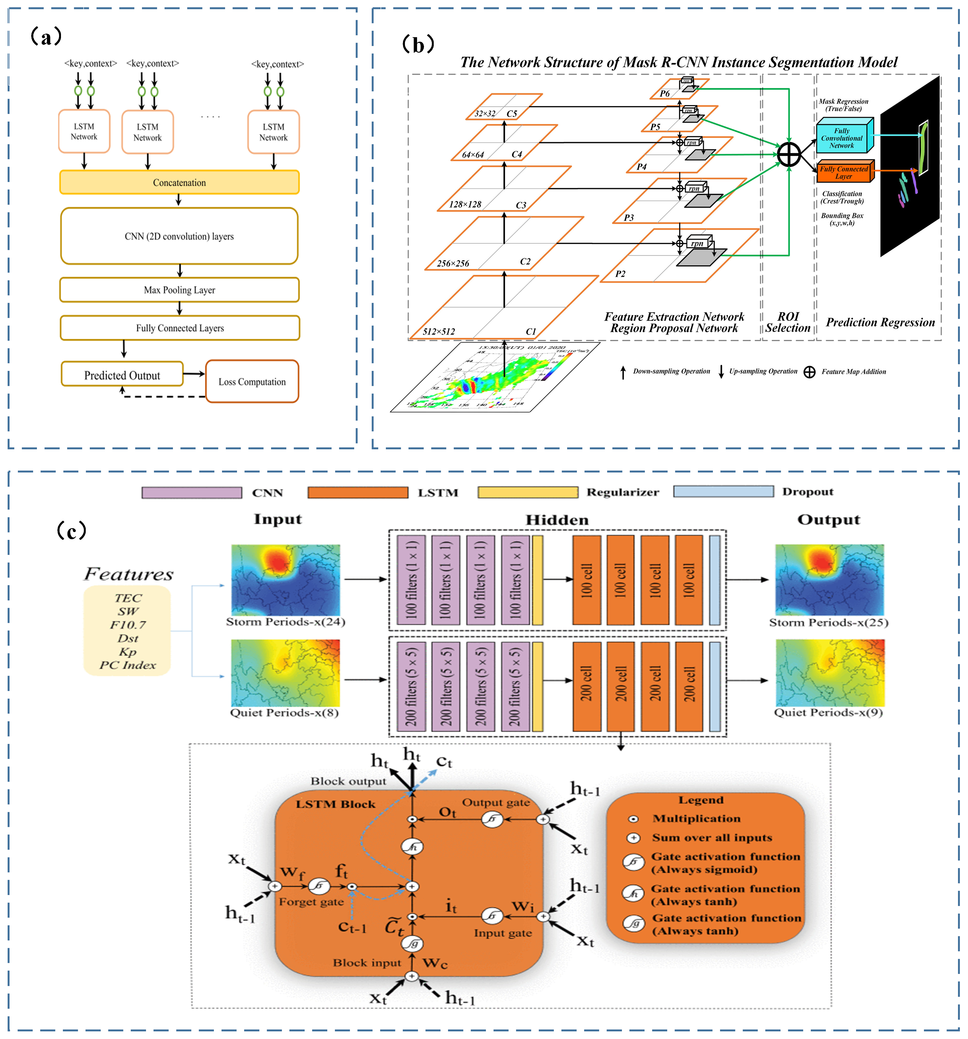
| Ren et al. [44] | Mixed-CNN-BiLSTM |
|
| Xia et al. [51] | ED-ConvLSTM |
|
| Boulch et al. [103] | CNN+RNN |
|
| Ruwali et al. [53] | LSTM-CNN |
|
| Li et al. [100] | ED-ConvLSTM |
|
| Tang et al. [104] | CNN-LSTM-Attention |
|
| Kaselimi et al. [101] | CNN-GRU |
|
| Xu et al. [102] | CNN-BiLSTM-TPA |
|
| Mao et al. [99] | CNN-LSTM |
|
3.3. Recurrent Neural Network (RNNs) and Long Short-Term Memory Network (LSTM)

| Source | Method | Main Features and Results |
|---|---|---|
| Liu et al. [9] | LSTM-NN |
|
| Sun et al. [112] | Bi-LSTM |
|
| Xie et al. [14] | Piecewise LSTM |
|
| Yuan et al. [106] | RNN |
|
| NATH et al. [113] | EEMD-LSTM |
|
| Ruwali et al. [53] | LSTM-CNN |
|
| Reddybattula et al. [6] | LSTM |
|
| Shi et al. [114] | ICEEMDAN-LSTM |
|
| Lu et al. [115] | Seq2Seq-LSTM-Attention |
|
3.4. Autoencoder and Generative Adversarial Network (GAN)
3.5. Comparative Performances of Global or Regional Models
4. Applications of Ionospheric Models Based on Deep Learning Techniques
4.1. Enhancing Navigation Service Quality
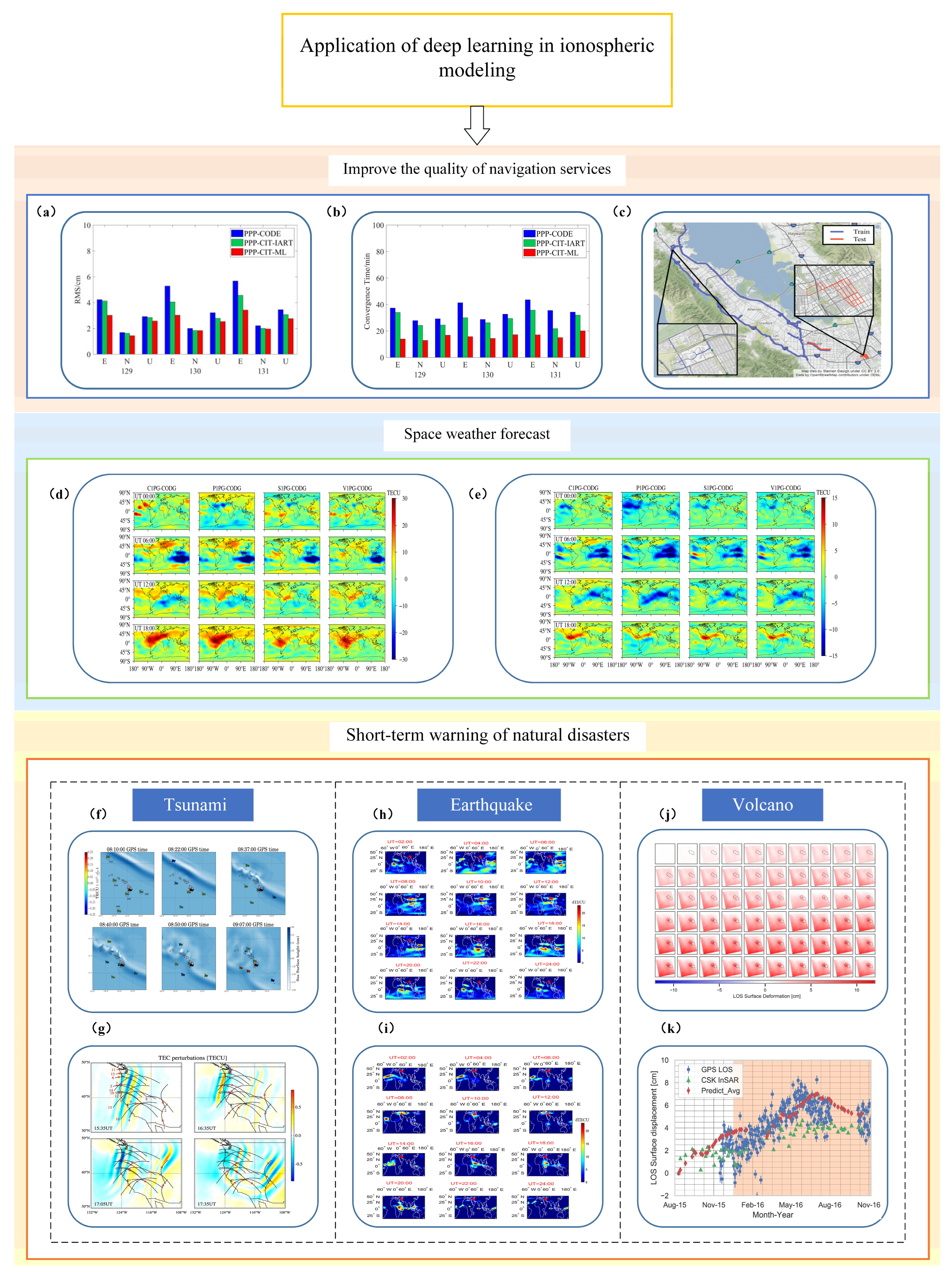
4.2. Space Weather Monitoring
4.3. Short-Term Early Warning of Major Natural Disasters
5. Conclusions and Prospects
- (1)
- Integrating multi-modal data fusion with deep learning effectively combines data from diverse sources, such as ground observations, satellite data, and space weather parameters, capturing the spatiotemporal dynamics of the ionosphere. For instance, the hybrid model RFGAN utilizes multi-source TEC data for global fusion, enhancing data integrity and prediction accuracy [144]. Furthermore, deep learning in multi-modal remote sensing data fusion has significantly improved the interpretability of Earth observation data [145]. Multi-modal networks like MANET, which combine meteorological and imagery data, enhance the accuracy of weather system classification [146]. These methods highlight deep learning’s advantages in multisource data fusion, contributing to more precise ionospheric modeling and prediction.
- (2)
- The integration of deep learning and transfer learning techniques in data-limited areas effectively addresses shortages and enhances predictive performance. Combining GANs with transfer learning significantly improves ionospheric modeling in data-scarce regions. GANs generate synthetic data that closely resembles real distributions, compensating for deficiencies and enhancing model stability in low-latitude areas [58]. Transfer learning, by utilizing pretrained models and fine-tuning them for specific domains, greatly enhances generalization and prediction accuracy [147]. This combination offers significant advantages in managing spatiotemporal inhomogeneity, thereby enhancing the precision and reliability of ionospheric predictions [148].
- (3)
- By integrating traditional physics-based models with deep learning techniques, hybrid models leverage the strengths of both approaches, enhancing the accuracy and feasibility of ionospheric modeling. This integration allows for the reliable application of physical features alongside deep learning’s ability to manage complex nonlinear data, improving model accuracy and stability. Such models excel in data-scarce environments and extreme space weather conditions, significantly enhancing the prediction accuracy of ionospheric TEC and other parameters [51,108]. This hybrid model has promising applications in creating robust real-time early warning systems and supporting navigation and communication.
- (4)
- Research on adaptive learning algorithms focuses on real-time adjustment of deep learning model parameters and structures to better handle the complex and unpredictable variations of the ionosphere. This includes online parameter tuning and trajectory tracking via the Lyapunov method, enhancing stability in nonlinear systems [149]. Integrating reinforcement learning techniques allows for dynamic adjustment of the action space and reward function, improving convergence speed and control stability of real-time tuning [150]. Additionally, adaptive activation functions optimize the learning process, accelerating convergence and enhancing accuracy in complex problem-solving [151]. These methods provide a solid foundation for improving the flexibility and responsiveness of models.
Author Contributions
Funding
Data Availability Statement
Conflicts of Interest
References
- Liu, J.; Wan, W.-X. Spatial-temporal distribution of the ionospheric perturbations prior to MS≥6.0 earthquakes in China main land. Chin. J. Geophys. 2014, 57, 2181–2189. (In Chinese) [Google Scholar]
- Tang, J.; Yao, Y.; Zhang, L. Temporal and Spatial Ionospheric Variations of 20 April 2013 Earthquake in Yaan, China. IEEE Geosci. Remote Sens. Lett. 2015, 12, 2242–2246. [Google Scholar] [CrossRef]
- Li, W.; Yang, F.; Yang, J.; Zhang, R.; Lin, J.; Zhao, D.; Hancock, C.M. Morphological Features of Severe Ionospheric Weather Associated with Typhoon Doksuri in 2023. Remote Sens. 2024, 16, 3375. [Google Scholar] [CrossRef]
- Li, W.; Zhu, H.; Feng, J.; Wu, X.; Tang, J.; Zhang, Z.; Chen, J. Asymmetric ionospheric fluctuations over the Circum-Pacific regions following the January 2022 Tonga volcanic eruption. Space Weather. 2023, 21, e2022SW003213. [Google Scholar] [CrossRef]
- Ren, X.; Zhao, B.; Ren, Z.; Xiong, B. Ionospheric TEC Prediction in China during Storm Periods Based on Deep Learning: Mixed CNN-BiLSTM Method. Remote Sens. 2024, 16, 3160. [Google Scholar] [CrossRef]
- Reddybattula, K.D.; Nelapudi, L.S.; Moses, M.; Devanaboyina, V.R.; Ali, M.A.; Jamjareegulgarn, P.; Panda, S.K. Ionospheric TEC Forecasting over an Indian Low Latitude Location Using Long Short-Term Memory (LSTM) Deep Learning Network. Universe 2022, 8, 562. [Google Scholar] [CrossRef]
- Dabbakuti, J.R.K.K.; Jacob, A.; Veeravalli, V.R.; Kallakunta, R.K. Implementation of IoT Analytics Ionospheric Forecasting System Based on Machine Learning and ThingSpeak. IET Radar Sonar Navig. 2020, 14, 341–347. [Google Scholar] [CrossRef]
- Li, X.; Zhou, C.; Tang, Q.; Zhao, J.; Zhang, F.; Xia, G.; Liu, Y. Forecasting Ionospheric foF2 Based on Deep Learning Method. Remote Sens. 2021, 13, 3849. [Google Scholar] [CrossRef]
- Liu, L.; Zou, S.; Yao, Y.; Wang, Z. Forecasting Global Ionospheric TEC Using Deep Learning Approach. Space Weather 2020, 18, e2020SW002501. [Google Scholar] [CrossRef]
- Ren, X.; Yang, P.; Liu, H.; Chen, J.; Liu, W. Deep Learning for Global Ionospheric TEC Forecasting: Different Approaches and Validation. Space Weather 2022, 20, e2021SW003011. [Google Scholar] [CrossRef]
- Klobuchar, J.A. Ionospheric Time-Delay Algorithm for Single-Frequency GPS Users. IEEE Trans. Aerosp. Electron. Syst. 1987, AES-23, 325–331. [Google Scholar] [CrossRef]
- Yuan, Y.; Wang, N.; Li, Z.; Huo, X. The BeiDou Global Broadcast Ionospheric Delay Correction Model (BDGIM) and Its Preliminary Performance Evaluation Results. Navigation 2019, 66, 55–69. [Google Scholar] [CrossRef]
- Prieto-Cerdeira, R.; Orús Pérez, R.; Breeuwer, E.; Lucas-Rodriguez, R.; Falcone, M. Performance of the Galileo Single-Frequency Ionospheric Correction During In-Orbit Validation. GPSworld 2014, 25, 53–58. [Google Scholar]
- Xie, T.; Dai, Z.; Zhu, X.; Chen, B.; Ran, C. LSTM-Based Short-Term Ionospheric TEC Forecast Model and Positioning Accuracy Analysis. GPS Solut. 2023, 27, 66. [Google Scholar] [CrossRef]
- Mohanty, A.; Gao, G. A Survey of Machine Learning Techniques for Improving Global Navigation Satellite Systems. EURASIP J. Adv. Signal Process. 2024, 2024, 73. [Google Scholar] [CrossRef]
- Srivani, I.; Siva Vara Prasad, G.; Venkata Ratnam, D. A Deep Learning-Based Approach to Forecast Ionospheric Delays for GPS Signals. IEEE Geosci. Remote Sens. Lett. 2019, 16, 1180–1184. [Google Scholar] [CrossRef]
- Yuan, Y.; Ou, J. An Improvement to Ionospheric Delay Correction for Single-Frequency GPS Users–the APR-I Scheme. J. Geod. 2001, 75, 331–336. [Google Scholar] [CrossRef]
- Xu, H.; Chen, X.; Ou, J.; Yuan, Y. Crowdsourcing RTK: A New GNSS Positioning Framework for Building Spatial High-Resolution Atmospheric Maps Based on Massive Vehicle GNSS Data. Satell. Navig. 2024, 5, 13. [Google Scholar] [CrossRef]
- Zhang, Z.; Wang, Y. A Spatiotemporal Model for Global Earthquake Prediction Based on Convolutional LSTM. IEEE Trans. Geosci. Remote Sens. 2023, 61, 5915712. [Google Scholar] [CrossRef]
- Uyanık, H.; Şentürk, E.; Akpınar, M.H.; Ozcelik, S.T.A.; Kokum, M.; Freeshah, M.; Sengur, A. A Multi-Input Convolutional Neural Networks Model for Earthquake Precursor Detection Based on Ionospheric Total Electron Content. Remote Sens. 2023, 15, 5690. [Google Scholar] [CrossRef]
- Saba, S.; Ahsan, F.; Mohsin, S. BAT-ANN Based Earthquake Prediction for Pakistan Region. Soft Comput. 2017, 21, 5805–5813. [Google Scholar] [CrossRef]
- Alfonsi, L.; Cesaroni, C.; Hernandez-Pajares, M.; Astafyeva, E.; Bufféral, S.; Elias, P.; Belehaki, A.; Ioanna, T.; Yang, H.; Guerra, M. Ionospheric Response to the 2020 Samos Earthquake and Tsunami. Earth Planets Space 2024, 76, 13. [Google Scholar] [CrossRef]
- Brissaud, Q.; Astafyeva, E. Near-Real-Time Detection of Co-Seismic Ionospheric Disturbances Using Machine Learning. Geophys. J. Int. 2022, 230, 2117–2130. [Google Scholar] [CrossRef]
- Peltier, W.R.; Hines, C.O. On the Possible Detection of Tsunamis by a Monitoring of the Ionosphere. J. Geophys. Res. 1896–1977 1976, 81, 1995–2000. [Google Scholar] [CrossRef]
- Savastano, G.; Komjathy, A.; Verkhoglyadova, O.; Mazzoni, A.; Crespi, M.; Wei, Y.; Mannucci, A.J. Real-Time Detection of Tsunami Ionospheric Disturbances with a Stand-Alone GNSS Receiver: A Preliminary Feasibility Demonstration. Sci. Rep. 2017, 7, 46607. [Google Scholar] [CrossRef] [PubMed]
- Constantinou, V.; Ravanelli, M.; Liu, H.; Bortnik, J. Deep Learning Driven Detection of Tsunami Related Internal GravityWaves: A Path Towards Open-Ocean Natural Hazards Detection. In Proceedings of the IEEE/CVF International Conference on Computer Vision Workshops (ICCVW), Paris, France, 2–6 October 2023; pp. 3748–3753. [Google Scholar] [CrossRef]
- Brengman, C.M.J.; Barnhart, W.D. Identification of Surface Deformation in InSAR Using Machine Learning. Geochem. Geophys. Geosyst. 2021, 22, e2020GC009204. [Google Scholar] [CrossRef]
- Tang, L. Ionospheric Disturbances of the January 15, 2022, Tonga Volcanic Eruption Observed Using the GNSS Network in New Zealand. GPS Solut. 2023, 27, 53. [Google Scholar] [CrossRef]
- Hickey, M.P.; Schubert, G.; Walterscheid, R.L. Propagation of Tsunami-Driven Gravity Waves into the Thermosphere and Ionosphere. J. Geophys. Res. Space Phys. 2009, 114, A08304. [Google Scholar] [CrossRef]
- Fadhillah, M.F.; Hakim, W.L.; Park, S.; Kim, D.; Park, Y.-C.; Kim, C.-H.; Lee, C.-W. Surface Deformation Simulation for InSAR Detection Using a Machine Learning Approach on the Hantangang River Volcanic Field: A Case Study on the Orisan Mountain. Front. Environ. Sci. 2022, 10, 968120. [Google Scholar] [CrossRef]
- Marchetti, D.; Zhu, K.; Zhang, H.; Zhima, Z.; Yan, R.; Shen, X.; Chen, W.; Cheng, Y.; He, X.; Wang, T.; et al. Clues of Lithosphere, Atmosphere and Ionosphere Variations Possibly Related to the Preparation of La Palma 19 September 2021 Volcano Eruption. Remote Sens. 2022, 14, 5001. [Google Scholar] [CrossRef]
- Bilitza, D.; Pezzopane, M.; Truhlik, V.; Altadill, D.; Reinisch, B.W.; Pignalberi, A. The International Reference Ionosphere Model: A Review and Description of an Ionospheric Benchmark. Rev. Geophys. 2022, 60, e2022RG000792. [Google Scholar] [CrossRef]
- Pongracic, B.; Wu, F.; Fathollahi, L.; Brčić, D. Midlatitude Klobuchar Correction Model Based on the K-Means Clustering of Ionospheric Daily Variations. GPS Solut. 2019, 23, 80. [Google Scholar] [CrossRef]
- Wang, C.; Xia, S.; Fan, L.; Shi, C.; Jing, G. Ionospheric Climate Index as a Driving Parameter for the NeQuick Model. Adv. Space Res. 2023, 71, 216–227. [Google Scholar] [CrossRef]
- Razin, M.R.G.; Voosoghi, B. Regional Ionosphere Modeling Using Spherical Cap Harmonics and Empirical Orthogonal Functions over Iran. Acta Geod. Geophys. 2017, 52, 19–33. [Google Scholar] [CrossRef]
- Zhou, C.; Yang, L.; Su, X.; Li, B. Neural Network-Based Ionospheric Modeling and Predicting—To Enhance High Accuracy GNSS Positioning and Navigation. Adv. Space Res. 2022, 70, 2878–2893. [Google Scholar] [CrossRef]
- Yuan, Y.; Ou, J. A Generalized Trigonometric Series Function Model for Determining Ionospheric Delay. Prog. Nat. Sci. 2004, 14, 1010–1014. [Google Scholar] [CrossRef]
- Asaly, S.; Gottlieb, L.-A.; Inbar, N.; Reuveni, Y. Using Support Vector Machine (SVM) with GPS Ionospheric TEC Estimations to Potentially Predict Earthquake Events. Remote Sens. 2022, 14, 2822. [Google Scholar] [CrossRef]
- Yuan, Y.; Tscherning, C.C.; Knudsen, P.; Xu, G.; Ou, J. The Ionospheric Eclipse Factor Method (IEFM) and Its Application to Determining the Ionospheric Delay for GPS. J. Geod. 2008, 82, 1–8. [Google Scholar] [CrossRef]
- Qian, L.; Burns, A.G.; Emery, B.A.; Foster, B.; Lu, G.; Maute, A.; Richmond, A.D.; Roble, R.G.; Solomon, S.C.; Wang, W. The NCAR TIE-GCM: A Community Model of the Coupled Thermosphere/Ionosphere System. In Proceedings of the Modeling the Ionosphere-Thermosphere System; Huba, J., Schunk, R., Khazanov, G., Eds.; Amer Geophysical Union: Washington, DC, USA, 2013; Volume 201, pp. 73–83. [Google Scholar]
- Tao, C.; Jin, H.; Miyoshi, Y.; Shinagawa, H.; Fujiwara, H.; Nishioka, M.; Ishii, M. Numerical Forecast of the Upper Atmosphere and Ionosphere Using GAIA. Earth Planets Space 2020, 72, 178. [Google Scholar] [CrossRef]
- Liu, H.-L.; Bardeen, C.G.; Foster, B.T.; Lauritzen, P.H.; Liu, J.; Lu, G.; Marsh, D.R.; Maute, A.; McInerney, J.M.; Pedatella, N.M.; et al. Development and Validation of the Whole Atmosphere Community Climate Model With Thermosphere and Ionosphere Extension (WACCM-X 2.0). J. Adv. Model. Earth Syst. 2018, 10, 381–402. [Google Scholar] [CrossRef]
- Rao, T.V.; Sridhar, M.; Ratnam, D.V.; Harsha, P.B.S.; Srivani, I. A Bidirectional Long Short-Term Memory-Based Ionospheric foF2 and hmF2 Models for a Single Station in the Low Latitude Region. IEEE Geosci. Remote Sens. Lett. 2022, 19, 8005405. [Google Scholar] [CrossRef]
- Ren, X.; Zhao, B.; Ren, Z.; Wang, Y.; Xiong, B. Deep Learning-Based Prediction of Global Ionospheric TEC During Storm Periods: Mixed CNN-BiLSTM Method. Space Weather 2024, 22, e2024SW003877. [Google Scholar] [CrossRef]
- Tian, P.; Yu, B.; Ye, H.; Xue, X.; Wu, J.; Chen, T. Estimation Model of Global Ionospheric Irregularities: An Artificial Intelligence Approach. Space Weather 2022, 20, e2022SW003160. [Google Scholar] [CrossRef]
- Bi, C.; Ren, P.; Yin, T.; Zhang, Y.; Li, B.; Xiang, Z. An Informer Architecture-Based Ionospheric foF2 Model in the Middle Latitude Region. IEEE Geosci. Remote Sens. Lett. 2022, 19, 1005305. [Google Scholar] [CrossRef]
- Tang, J.; Ding, M.; Yang, D.; Fan, C.; Khonsari, N.; Mao, W. Different Data-Driven Prediction of Global Ionospheric TEC Using Deep Learning Methods. Int. J. Appl. Earth Obs. Geoinf. 2024, 130, 103889. [Google Scholar] [CrossRef]
- Tang, J.; Yang, D.; Ding, M. Forecasting Ionospheric foF2 Using Bidirectional LSTM and Attention Mechanism. Space Weather 2023, 21, e2023SW003508. [Google Scholar] [CrossRef]
- Yang, D.; Fang, H. Forecasting of Global Ionospheric TEC Using a Deep Learning Approach. GPS Solut. 2023, 27, 74. [Google Scholar] [CrossRef]
- An, X.; Meng, X.; Jiang, W.; Chen, H.; He, Q.; Xi, R. Global Ionosphere Estimation Based on Data Fusion From Multisource: Multi-GNSS, IRI Model, and Satellite Altimetry. J. Geophys. Res. Space Phys. 2019, 124, 6012–6028. [Google Scholar] [CrossRef]
- Xia, G.; Zhang, F.; Wang, C.; Zhou, C. ED-ConvLSTM: A Novel Global Ionospheric Total Electron Content Medium-Term Forecast Model. Space Weather 2022, 20, e2021SW002959. [Google Scholar] [CrossRef]
- Weng, J.; Liu, Y.; Wang, J. A Model-Assisted Combined Machine Learning Method for Ionospheric TEC Prediction. Remote Sens. 2023, 15, 2953. [Google Scholar] [CrossRef]
- Ruwali, A.; Kumar, A.J.S.; Prakash, K.B.; Sivavaraprasad, G.; Ratnam, D.V. Implementation of Hybrid Deep Learning Model (LSTM-CNN) for Ionospheric TEC Forecasting Using GPS Data. IEEE Geosci. Remote Sens. Lett. 2021, 18, 1004–1008. [Google Scholar] [CrossRef]
- Tang, J.; Zhong, Z.; Hu, J.; Wu, X. Forecasting Regional Ionospheric TEC Maps over China Using BiConvGRU Deep Learning. Remote Sens. 2023, 15, 3405. [Google Scholar] [CrossRef]
- Roma-Dollase, D.; Hernández-Pajares, M.; Krankowski, A.; Kotulak, K.; Ghoddousi-Fard, R.; Yuan, Y.; Li, Z.; Zhang, H.; Shi, C.; Wang, C.; et al. Consistency of Seven Different GNSS Global Ionospheric Mapping Techniques during One Solar Cycle. J. Geod. 2018, 92, 691–706. [Google Scholar] [CrossRef]
- Chen, Z.; Wang, S.; Fang, G.; Wang, J. Ionograms Denoising via Curvelet Transform. Adv. Space Res. 2013, 52, 1289–1296. [Google Scholar] [CrossRef]
- Wang, C.; Liu, L.; Chen, L.; Feng, J.; Zhao, H.-S. Improved TEC Retrieval Based on Spaceborne PolSAR Data. Radio Sci. 2017, 52, 288–304. [Google Scholar] [CrossRef]
- Yang, D.; Fang, H.; Liu, Z. Completion of Global Ionospheric TEC Maps Using a Deep Learning Approach. J. Geophys. Res. Space Phys. 2022, 127, e2022JA030326. [Google Scholar] [CrossRef]
- Lin, X.; Chao, S.; Yan, D.; Guo, L.; Liu, Y.; Li, L. Multi-Sensor Data Fusion Method Based on Self-Attention Mechanism. Appl. Sci. 2023, 13, 11992. [Google Scholar] [CrossRef]
- Richmond, A.D.; Ridley, E.C.; Roble, R.G. A Thermosphere/Ionosphere General Circulation Model with Coupled Electrodynamics. Geophys. Res. Lett. 1992, 19, 601–604. [Google Scholar] [CrossRef]
- Bilitza, D. IRI the International Standard for the Ionosphere. Adv. Radio Sci. 2018, 16, 1–11. [Google Scholar] [CrossRef]
- Wang, C.; Hajj, G.; Pi, X.; Rosen, I.G.; Wilson, B. Development of the Global Assimilative Ionospheric Model. Radio Sci. 2004, 39, 1–11. [Google Scholar] [CrossRef]
- Komjathy, A.; Wilson, B.; Pi, X.; Akopian, V.; Dumett, M.; Iijima, B.; Verkhoglyadova, O.; Mannucci, A.J. JPL/USC GAIM: On the Impact of Using COSMIC and Ground-Based GPS Measurements to Estimate Ionospheric Parameters. J. Geophys. Res. Space Phys. 2010, 115, A02307. [Google Scholar] [CrossRef]
- Bust, G.S.; Garner, T.W.; Gaussiran II, T.L. Ionospheric Data Assimilation Three-Dimensional (IDA3D): A Global, Multisensor, Electron Density Specification Algorithm. J. Geophys. Res. Space Phys. 2004, 109, A11312. [Google Scholar] [CrossRef]
- Mengist, C.K.; Ssessanga, N.; Jeong, S.-H.; Kim, J.-H.; Kim, Y.H.; Kwak, Y.-S. Assimilation of Multiple Data Types to a Regional Ionosphere Model With a 3D-Var Algorithm (IDA4D). Space Weather 2019, 17, 1018–1039. [Google Scholar] [CrossRef]
- Jeong, S.-H.; Kim, Y.H.; Kim, J.-H.; Kwak, Y.-S. A Regional Ionospheric Assimilation Study with GPS and COSMIC Measurements Using a 3D-Var Algorithm (IDA4D). Adv. Space Res. 2022, 69, 2489–2500. [Google Scholar] [CrossRef]
- Inyurt, S.; Sekertekin, A. Modeling and Predicting Seasonal Ionospheric Variations in Turkey Using Artificial Neural Network (ANN). Astrophys. Space Sci. 2019, 364, 62. [Google Scholar] [CrossRef]
- Habarulema, J.B.; McKinnell, L.-A.; Cilliers, P.J. Prediction of Global Positioning System Total Electron Content Using Neural Networks over South Africa. J. Atmos. Sol.-Terr. Phys. 2007, 69, 1842–1850. [Google Scholar] [CrossRef]
- Hernández-Pajares, M.; Juan, J.M.; Sanz, J. Neural Network Modeling of the Ionospheric Electron Content at Global Scale Using GPS Data. Radio Sci. 1997, 32, 1081–1089. [Google Scholar] [CrossRef]
- Cander, L.R. Artificial Neural Network Applications in Ionospheric Studies. Ann. Geophys. 1998, 41, 5–6. [Google Scholar] [CrossRef]
- Rumelhart, D.E.; Hinton, G.E.; Williams, R.J. Learning Representations by Back-Propagating Errors. Nature 1986, 323, 533–536. [Google Scholar] [CrossRef]
- Gu, J.; Wang, Z.; Kuen, J.; Ma, L.; Shahroudy, A.; Shuai, B.; Liu, T.; Wang, X.; Wang, G.; Cai, J.; et al. Recent Advances in Convolutional Neural Networks. Pattern Recognit. 2018, 77, 354–377. [Google Scholar] [CrossRef]
- Kail, R.; Burnaev, E.; Zaytsev, A. Recurrent Convolutional Neural Networks Help to Predict Location of Earthquakes. IEEE Geosci. Remote Sens. Lett. 2022, 19, 8019005. [Google Scholar] [CrossRef]
- Sun, W.; Xu, L.; Huang, X.; Zhang, W.; Yuan, T.; Chen, Z.; Yan, Y. Forecasting of Ionospheric Vertical Total Electron Content (TEC) Using LSTM Networks. In Proceedings of the 2017 International Conference on Machine Learning and Cybernetics (ICMLC), Ningbo, China, 9–12 July 2017; Volume 2, pp. 340–344. [Google Scholar] [CrossRef]
- Goodfellow, I.; Pouget-Abadie, J.; Mirza, M.; Xu, B.; Warde-Farley, D.; Ozair, S.; Courville, A.; Bengio, Y. Generative Adversarial Networks. Commun. ACM 2020, 63, 139–144. [Google Scholar] [CrossRef]
- Chen, Z.; Liao, W.; Li, H.; Wang, J.; Deng, X.; Hong, S. Prediction of Global Ionospheric TEC Based on Deep Learning. Space Weather 2022, 20, e2021SW002854. [Google Scholar] [CrossRef]
- Oyeyemi, E.O.; Poole, A.W.V.; McKinnell, L.A. On the Global Model for foF2 Using Neural Networks. Radio Sci. 2005, 40, RS6011. [Google Scholar] [CrossRef]
- Habarulema, J. A Feasibility Study into Total Electron Content Prediction Using Neural Networks. Doctoral Dissertation, Rhodes University, Makhanda, South Africa, 2007. [Google Scholar]
- Maruyama, T. Solar Proxies Pertaining to Empirical Ionospheric Total Electron Content Models. J. Geophys. Res. Space Phys. 2010, 115, A04306. [Google Scholar] [CrossRef]
- Zhao, X.; Ning, B.; Liu, L.; Song, G. A Prediction Model of Short-Term Ionospheric foF2 Based on AdaBoost. Adv. Space Res. 2014, 53, 387–394. [Google Scholar] [CrossRef]
- Pu, Y.; Chen, Y.; Dong, Y.; Zhang, K.; Wang, F.; Xi, X. Prediction the Diurnal Variation of VLF Waves in Earth-Ionosphere Waveguide Based on BPNN-TL Method. IEEE Antennas Wirel. Propag. Lett. 2024, 1–5. [Google Scholar] [CrossRef]
- Wu, J.; Chen, J.; Gu, L. Alternative Combination of Improved Particle Swarm and Back Propagation Neural Network. In Proceedings of the 2010 Sixth International Conference on Natural Computation, Yantai, China, 10–12 August 2010; Volume 1, pp. 75–78. [Google Scholar] [CrossRef]
- Xiao, C.; Hu, X. Applying Artificial Neural Networks to Modeling the Middle Atmosphere. Adv. Atmos. Sci. 2010, 27, 883–890. [Google Scholar] [CrossRef]
- Huang, Z.; Li, Q.B.; Yuan, H. Forecasting of Ionospheric Vertical TEC 1-h Ahead Using a Genetic Algorithm and Neural Network. Adv. Space Res. 2015, 55, 1775–1783. [Google Scholar] [CrossRef]
- Xu, L.; Gao, J.; Li, Z.; Shu, M.; Yang, X.; Zhang, G. A New Flexible Model to Calibrate Single-Layer Height for Ionospheric Modeling Using a Neural Network Model. GPS Solut. 2023, 27, 106. [Google Scholar] [CrossRef]
- Poole, A.W.V.; McKinnell, L.-A. On the Predictability of f0F2 Using Neural Networks. Radio Sci. 2000, 35, 225–234. [Google Scholar] [CrossRef]
- Lin, J.-W.; Chao, C.-T.; Chiou, J.-S. Determining Neuronal Number in Each Hidden Layer Using Earthquake Catalogues as Training Data in Training an Embedded Back Propagation Neural Network for Predicting Earthquake Magnitude. IEEE Access 2018, 6, 52582–52597. [Google Scholar] [CrossRef]
- Lei, J.; Rui, S.U.N.; Zhengwu, L.I.U.; Cheng, X.U.; Dida, L.; Dezhen, H.U. Modeling and Accuracy Analysis of GNSS Ionospheric Error in EU-China Based on GA-BP. J. Beijing Univ. Aeronaut. Astronaut. 2022, 49, 1533–1542. [Google Scholar] [CrossRef]
- Zhang, Y.; Zhen, W.; Chen, L.; Ou, M.; Yu, X.; Wang, Y.; Chen, L. Ionospheric TEC Storm Prediction Based on AdaBoost-BP. In Proceedings of the 2022 Cross Strait Radio Science & Wireless Technology Conference (CSRSWTC), Haidian, China, 17–18 December 2022; pp. 1–3. [Google Scholar] [CrossRef]
- Long, F.; Gao, C.; Dong, Y. Modeling and Predicting the Ionospheric Total Electron Content Over Western China With Machine Learning. In Proceedings of the 2021 IEEE 12th Annual Information Technology, Electronics and Mobile Communication Conference (IEMCON), Vancouver, BC, Canada, 27–30 October 2021; pp. 1052–1057. [Google Scholar] [CrossRef]
- Fang, Z.; Shen, J.; Zhou, X. Prediction of foF2 Frequency Based on BP Neural Network with Single Point Extrapolation. In Proceedings of the 2022 IEEE 6th Information Technology and Mechatronics Engineering Conference (ITOEC), Chongqing, China, 4–6 March 2022; Volume 6, pp. 1808–1812. [Google Scholar] [CrossRef]
- Chen, X.; Yang, H.; Gao, J.; Yu, C. Prediction of Ionospheric F2 Layer Heights Obtained from HFSWR during Typhoons Utilizing GA-BP Neural Network Model. In Proceedings of the 2024 Photonics & Electromagnetics Research Symposium (PIERS), Chengdu, China, 21–25 April 2024; pp. 1–7. [Google Scholar] [CrossRef]
- Lecun, Y.; Bottou, L.; Bengio, Y.; Haffner, P. Gradient-Based Learning Applied to Document Recognition. Proc. IEEE 1998, 86, 2278–2324. [Google Scholar] [CrossRef]
- Krizhevsky, A.; Sutskever, I.; Hinton, G.E. ImageNet Classification with Deep Convolutional Neural Networks. Commun. ACM 2017, 60, 84–90. [Google Scholar] [CrossRef]
- Szegedy, C.; Liu, W.; Jia, Y.; Sermanet, P.; Reed, S.; Anguelov, D.; Erhan, D.; Vanhoucke, V.; Rabinovich, A. Going Deeper With Convolutions. In Proceedings of the IEEE Conference on Computer Vision and Pattern Recognition, Boston, MA, USA, 7–12 June 2015; pp. 1–9. [Google Scholar] [CrossRef]
- He, K.; Zhang, X.; Ren, S.; Sun, J. Deep Residual Learning for Image Recognition. In Proceedings of the IEEE Conference on Computer Vision and Pattern Recognition, Las Vegas, NV, USA, 27–30 June 2016; pp. 770–778. [Google Scholar] [CrossRef]
- Liu, P.; Yokoyama, T.; Fu, W.; Yamamoto, M. Statistical Analysis of Medium-Scale Traveling Ionospheric Disturbances Over Japan Based on Deep Learning Instance Segmentation. Space Weather 2022, 20, e2022SW003151. [Google Scholar] [CrossRef]
- Li, W.; Zhu, H.; Shi, S.; Zhao, D.; Shen, Y.; He, C. Modeling China’s Sichuan-Yunnan’s Ionosphere Based on Multichannel WOA-CNN-LSTM Algorithm. IEEE Trans. Geosci. Remote Sens. 2024, 62, 5705018. [Google Scholar] [CrossRef]
- Mao, S.; Li, H.; Zhang, Y.; Shi, Y. Prediction of Ionospheric Electron Density Distribution Based on CNN-LSTM Model. IEEE Geosci. Remote Sens. Lett. 2024, 21, 1003305. [Google Scholar] [CrossRef]
- Li, L.; Liu, H.; Le, H.; Yuan, J.; Shan, W.; Han, Y.; Yuan, G.; Cui, C.; Wang, J. Spatiotemporal Prediction of Ionospheric Total Electron Content Based on ED-ConvLSTM. Remote Sens. 2023, 15, 3064. [Google Scholar] [CrossRef]
- Kaselimi, M.; Doulamis, N.; Voulodimos, A.; Doulamis, A.; Delikaraoglou, D. Spatio-Temporal Ionospheric TEC Prediction Using a Deep CNN-GRU Model on GNSS Measurements. In Proceedings of the 2021 IEEE International Geoscience and Remote Sensing Symposium IGARSS, Brussels, Belgium, 11–16 July 2021; pp. 8317–8320. [Google Scholar] [CrossRef]
- Xu, B.; Huang, W.; Ren, P.; Li, Y.; Xiang, Z. Modeling and Forecasting Ionospheric foF2 Variation Based on CNN-BiLSTM-TPA during Low- and High-Solar Activity Years. Remote Sens. 2024, 16, 3249. [Google Scholar] [CrossRef]
- Boulch, A.; Cherrier, N.; Castaings, T. Ionospheric Activity Prediction Using Convolutional Recurrent Neural Networks. arXiv 2018, arXiv:1810.13273. [Google Scholar]
- Tang, J.; Li, Y.; Ding, M.; Liu, H.; Yang, D.; Wu, X. An Ionospheric TEC Forecasting Model Based on a CNN-LSTM-Attention Mechanism Neural Network. Remote Sens. 2022, 14, 2433. [Google Scholar] [CrossRef]
- Hopfield, J.J. Neural Networks and Physical Systems with Emergent Collective Computational Abilities. Proc. Natl. Acad. Sci. USA 1982, 79, 2554–2558. [Google Scholar] [CrossRef] [PubMed]
- Tianjiao, Y.; Yanhong, C.; Siqing, L.I.U.; Jiancun, G. Prediction Model for Ionospheric Total Electron Content Based on Deep Learning Recurrent Neural Networkormalsize. Chin. J. Space Sci. 2018, 38, 48–57. [Google Scholar] [CrossRef]
- Hochreiter, S.; Schmidhuber, J. Long Short-Term Memory. Neural Comput. 1997, 9, 1735–1780. [Google Scholar] [CrossRef] [PubMed]
- Tang, R.; Zeng, F.; Chen, Z.; Wang, J.-S.; Huang, C.-M.; Wu, Z. The Comparison of Predicting Storm-Time Ionospheric TEC by Three Methods: ARIMA, LSTM, and Seq2Seq. Atmosphere 2020, 11, 316. [Google Scholar] [CrossRef]
- Wen, Z.; Li, S.; Li, L.; Wu, B.; Fu, J. Ionospheric TEC Prediction Using Long Short-Term Memory Deep Learning Network. Astrophys. Space Sci. 2021, 366, 3. [Google Scholar] [CrossRef]
- Kaselimi, M.; Voulodimos, A.; Doulamis, N.; Doulamis, A.; Delikaraoglou, D. A Causal Long Short-Term Memory Sequence to Sequence Model for TEC Prediction Using GNSS Observations. Remote Sens. 2020, 12, 1354. [Google Scholar] [CrossRef]
- Li, D.; Jin, Y.; Wu, F.; Zhao, J.; Min, P.; Luo, X. A Hybrid Model for TEC Prediction Using BiLSTM and PSO-LSSVM. Adv. Space Res. 2024, 74, 303–318. [Google Scholar] [CrossRef]
- Sun, W.; Xu, L.; Huang, X.; Zhang, W.; Yuan, T.; Yan, Y. Bidirectional LSTM for Ionospheric Vertical Total Electron Content (TEC) Forecasting. In Proceedings of the 2017 IEEE Visual Communications and Image Processing (VCIP), St. Petersburg, FL, USA, 10–13 December 2017; pp. 1–4. [Google Scholar] [CrossRef]
- Nath, S.; Chetia, B.; Kalita, S. Ionospheric TEC Prediction Using Hybrid Method Based on Ensemble Empirical Mode Decomposition (EEMD) and Long Short-Term Memory (LSTM) Deep Learning Model over India. Adv. Space Res. 2023, 71, 2307–2317. [Google Scholar] [CrossRef]
- Shi, Y.; Yang, C.; Wang, J.; Meng, F. A Hybrid Deep Learning-Based Short-Term Forecast Model for Ionospheric foF2 in East Asia Region. Adv. Space Res. 2024, 75, 988–1002. [Google Scholar] [CrossRef]
- Lu, Z.; Xu, K.; Wang, H.; Du, K. A Seq2Seq-LSTM-Attention Model for Ionospheric foF2 Prediction in the Middle Latitude Region. In Proceedings of the 2024 9th International Conference on Signal and Image Processing (ICSIP), Nanjing, China, 12–14 July 2024; pp. 221–225. [Google Scholar] [CrossRef]
- Abri, R.; Abri, S.; Artuner, H.; Cetin, S. Predicting Earthquakes with Ionospheric Data: A Hybrid Approach Utilizing Deep AutoEncoder and LSTM Networks. In Proceedings of the 2024 IEEE 3rd International Conference on Computing and Machine Intelligence (ICMI), Mt Pleasant, MI, USA, 13–14 April 2024; pp. 1–5. [Google Scholar] [CrossRef]
- Reid, J.; Liu, J.; Ananthabhotla, B. QuakeCast, an Earthquake Forecasting System Using Ionospheric Anomalies and Machine Learning. Authorea Prepr. 2021, 1–19. [Google Scholar] [CrossRef]
- Pan, Y.; Jin, M.; Zhang, S.; Deng, Y. TEC Map Completion Through a Deep Learning Model: SNP-GAN. Space Weather 2021, 19, e2021SW002810. [Google Scholar] [CrossRef]
- Yang, K.; Liu, Y. Global Ionospheric Total Electron Content Completion with a GAN-Based Deep Learning Framework. Remote Sens. 2022, 14, 6059. [Google Scholar] [CrossRef]
- Pan, Y.; Jin, M.; Zhang, S.; Deng, Y. TEC Map Completion Using DCGAN and Poisson Blending. Space Weather 2020, 18, e2019SW002390. [Google Scholar] [CrossRef]
- Li, L.; Liu, H.; Le, H.; Yuan, J.; Wang, H.; Chen, Y.; Shan, W.; Ma, L.; Cui, C. ED-AttConvLSTM: An Ionospheric TEC Map Prediction Model Using Adaptive Weighted Spatiotemporal Features. Space Weather 2024, 22, e2023SW003740. [Google Scholar] [CrossRef]
- Bilitza, D.; Altadill, D.; Truhlik, V.; Shubin, V.; Galkin, I.; Reinisch, B.; Huang, X. International Reference Ionosphere 2016: From Ionospheric Climate to Real-Time Weather Predictions. Space Weather 2017, 15, 418–429. [Google Scholar] [CrossRef]
- Chen, P.; Zheng, D.; Nie, W.; Ye, F.; Long, S.; He, C.; Liao, M.; Xie, J. Precise Point Positioning (PPP) Based on the Machine Learning-Based Ionospheric Tomography. Adv. Space Res. 2024, 74, 4835–4848. [Google Scholar] [CrossRef]
- Shi, S.; Zhang, K.; Shi, J.; Hu, A.; Zhao, D.; Shi, Z.; Sun, P.; Wu, H.; Wu, S. Modeling TEC Maps Over China Using Particle Swarm Optimization Neural Networks and Long-Term Ground-Based GPS, COSMIC, and Fengyun Data. Space Weather 2023, 21, e2022SW003357. [Google Scholar] [CrossRef]
- Kanhere, A.V.; Gupta, S.; Akshay, S.; Gao, G. Improving GNSS Positioning Using Neural-Network-Based Corrections. Navig. J. Inst. Navig. 2022, 69, navi.548. [Google Scholar] [CrossRef]
- Meng, X.; Komjathy, A.; Verkhoglyadova, O.P.; Yang, Y.-M.; Deng, Y.; Mannucci, A.J. A New Physics-Based Modeling Approach for Tsunami-Ionosphere Coupling. Geophys. Res. Lett. 2015, 42, 4736–4744. [Google Scholar] [CrossRef]
- Tariq, M.A.; Shah, M.; Hernández-Pajares, M.; Iqbal, T. Pre-Earthquake Ionospheric Anomalies before Three Major Earthquakes by GPS-TEC and GIM-TEC Data during 2015–2017. Adv. Space Res. 2019, 63, 2088–2099. [Google Scholar] [CrossRef]
- Sun, J.; Wauthier, C.; Stephens, K.; Gervais, M.; Cervone, G.; La Femina, P.; Higgins, M. Automatic Detection of Volcanic Surface Deformation Using Deep Learning. J. Geophys. Res. Solid Earth 2020, 125, e2020JB019840. [Google Scholar] [CrossRef]
- Li, W.; Wu, X. An Ionospheric Total Electron Content Model with a Storm Option over Japan Based on a Multi-Layer Perceptron Neural Network. Atmosphere. 2023, 14, 634. [Google Scholar] [CrossRef]
- Zewdie, G.K.; Valladares, C.; Cohen, M.B.; Lary, D.J.; Ramani, D.; Tsidu, G.M. Data-Driven Forecasting of Low-Latitude Ionospheric Total Electron Content Using the Random Forest and LSTM Machine Learning Methods. Space Weather 2021, 19, e2020SW002639. [Google Scholar] [CrossRef]
- Li, W.; Zhao, D.; Feng, J.; Wu, X.; Zhang, Z. Spatial Development of Strong Storm-Induced Ionospheric Perturbations during 25–27 August 2018. Remote Sens. 2023, 15, 2549. [Google Scholar] [CrossRef]
- Astafyeva, E. Ionospheric Detection of Natural Hazards. Rev. Geophys. 2019, 57, 1265–1288. [Google Scholar] [CrossRef]
- Foroodi, Z.; Alizadeh, M.; Schuh, H.; Tsai, L.-C. Alternative Approach for Tsunami Early Warning Indicated by Gravity Wave Effects on Ionosphere. Remote Sens. 2021, 13, 2150. [Google Scholar] [CrossRef]
- Verhulst, T.G.W.; Altadill, D.; Barta, V.; Belehaki, A.; Burešová, D.; Cesaroni, C.; Galkin, I.; Guerra, M.; Ippolito, A.; Herekakis, T.; et al. Multi-Instrument Detection in Europe of Ionospheric Disturbances Caused by the 15 January 2022 Eruption of the Hunga Volcano. J. Space Weather Space Clim. 2022, 12, 35. [Google Scholar] [CrossRef]
- Kakinami, Y.; Kamogawa, M.; Tanioka, Y.; Watanabe, S.; Gusman, A.R.; Liu, J.-Y.; Watanabe, Y.; Mogi, T. Tsunamigenic Ionospheric Hole. Geophys. Res. Lett. 2012, 39, L00G27. [Google Scholar] [CrossRef]
- Canário, J.P.; Mello, R.; Curilem, M.; Huenupan, F.; Rios, R. In-Depth Comparison of Deep Artificial Neural Network Architectures on Seismic Events Classification. J. Volcanol. Geotherm. Res. 2020, 401, 106881. [Google Scholar] [CrossRef]
- Bueno, A.; Benítez, C.; De Angelis, S.; Díaz Moreno, A.; Ibáñez, J.M. Volcano-Seismic Transfer Learning and Uncertainty Quantification With Bayesian Neural Networks. IEEE Trans. Geosci. Remote Sens. 2020, 58, 892–902. [Google Scholar] [CrossRef]
- Akhoondzadeh, M.; De Santis, A.; Marchetti, D.; Wang, T. Developing a Deep Learning-Based Detector of Magnetic, Ne, Te and TEC Anomalies from Swarm Satellites: The Case of Mw 7.1 2021 Japan Earthquake. Remote Sens. 2022, 14, 1582. [Google Scholar] [CrossRef]
- Salazar, A.; Arroyo, R.; Pérez, N.; Benítez, D. Deep-Learning for Volcanic Seismic Events Classification. In Proceedings of the 2020 IEEE Colombian Conference on Applications of Computational Intelligence (IEEE ColCACI 2020), Cali, Colombia, 7–8 August 2020; pp. 1–6. [Google Scholar] [CrossRef]
- Massinas, B.A.; Doulamis, A.; Doulamis, N.; Protopapadakis, E.; Paradissis, D. Deep Convolutional Neural Networks for Modeling Patterns of Spaceborne Interferometric SAR Systems Signals. In AIAA SPACE and Astronautics Forum and Exposition; American Institute of Aeronautics and Astronautics: Reston VA, USA, 2017. [Google Scholar] [CrossRef]
- Konstantaras, A. Deep Learning and Parallel Processing Spatio-Temporal Clustering Unveil New Ionian Distinct Seismic Zone. Informatics 2020, 7, 39. [Google Scholar] [CrossRef]
- Mignan, A.; Broccardo, M. A Deeper Look into ‘Deep Learning of Aftershock Patterns Following Large Earthquakes’: Illustrating First Principles in Neural Network Physical Interpretability. In Proceedings of the Advances in Computational Intelligence; Springer: Cham, Sitzerland, 2019; pp. 3–14. [Google Scholar]
- Li, Y.; Zhou, B.; Shen, S.; Lu, W.; Tang, C.; Li, S.; Su, Y.; Dai, S.; Fang, G. The Lunar Regolith Structure and Electromagnetic Properties of Chang’E-5 Landing Site. Remote Sens. 2022, 14, 4539. [Google Scholar] [CrossRef]
- Chen, Z.; Zhou, K.; Li, H.; Wang, J.; Ouyang, Z.; Deng, X. Autoencoders. Space Weather 2023, 21, e2022SW003341. [Google Scholar] [CrossRef]
- Li, J.; Hong, D.; Gao, L.; Yao, J.; Zheng, K.; Zhang, B.; Chanussot, J. Deep Learning in Multimodal Remote Sensing Data Fusion: A Comprehensive Review. Int. J. Appl. Earth Obs. Geoinf. 2022, 112, 102926. [Google Scholar] [CrossRef]
- Bai, C.; Zhao, D.; Zhang, M.; Zhang, J. Multimodal Information Fusion for Weather Systems and Clouds Identification From Satellite Images. IEEE J. Sel. Top. Appl. Earth Obs. Remote Sens. 2022, 15, 7333–7345. [Google Scholar] [CrossRef]
- Lin, F.; Chen, J.; Ding, G.; Jiao, Y.; Sun, J.; Wang, H. Spectrum Prediction Based on GAN and Deep Transfer Learning: A Cross-Band Data Augmentation Framework. China Commun. 2021, 18, 18–32. [Google Scholar] [CrossRef]
- Wang, B.; Kato, S.; Kano, M. GAN-Based Homogenous Transfer Learning Method for Regression Problems. In Proceedings of the 2023 IEEE Conference on Control Technology and Applications (CCTA), Bridgetown, Barbados, 16–18 August 2023; pp. 85–90. [Google Scholar] [CrossRef]
- Sun, R.; Greene, M.L.; Le, D.M.; Bell, Z.I.; Chowdhary, G.; Dixon, W.E. Lyapunov-Based Real-Time and Iterative Adjustment of Deep Neural Networks. IEEE Control Syst. Lett. 2022, 6, 193–198. [Google Scholar] [CrossRef]
- Detroja, K.P. Parameterized Adaptive Controller Design Using Reinforcement Learning and Deep Neural Networks. In Proceedings of the 2022 Eighth Indian Control Conference (ICC), Chennai, India, 14–16 December 2022; pp. 121–126. [Google Scholar] [CrossRef]
- Jagtap, A.D.; Kawaguchi, K.; Karniadakis, G.E. Adaptive Activation Functions Accelerate Convergence in Deep and Physics-Informed Neural Networks. J. Comput. Phys. 2020, 404, 109136. [Google Scholar] [CrossRef]


| Date Type | Affiliations | Date Access URL |
|---|---|---|
| GNSS Networks | Australian Space Weather Services | https://downloads.sws.bom.gov.au/wdc/gnss/data/, accessed on 1 July 2024 |
| Can-Net | https://www.can-net.ca/, accessed on 1 July 2024 | |
| Canadian High Arctic Ionospheric Network | http://chain.physics.unb.ca/chain/pages/data_download, accessed on 1 July 2024 | |
| Crustal Dynamics Data Information System | https://cddis.nasa.gov/archive/gnss/data/daily/, accessed on 1 July 2024 | |
| Dutch Permanent GNSS Array | http://gnss1.tudelft.nl/dpga/rinex, accessed on 1 July 2024 | |
| GeoNet New Zealand | https://www.geonet.org.nz/data/types/geodetic, accessed on 1 July 2024 | |
| INGV-Rete Integrata Nazionale GPS (RING) | http://ring.gm.ingv.it/, accessed on 1 July 2024 | |
| Institute of Geodynamics, National Observatory of Athens | https://www.gein.noa.gr/services/GPSData/, accessed on 1 July 2024 | |
| Instituto Tecnologico Agrario de Castilla y Leon | ftp://ftp.itacyl.es/RINEX/, accessed on 1 July 2024 | |
| International GNSS Service(IGS), UNAVCO | https://www.unavco.org/data/gps-gnss/gps-gnss.html, accessed on 1 July 2024. | |
| National Geodetic Survey | https://geodesy.noaa.gov/corsdata/, accessed on 1 July 2024. | |
| Pacific Northwest Geodetic Array (PANGA) | https://www.geodesy.org/about, accessed on 1 July 2024. | |
| Scripps Orbit and Permanent Array Center | http://garner.ucsd.edu/, accessed on 1 July 2024. | |
| SWEPOS Sweden | https://swepos.lantmateriet.se/, accessed on 1 July 2024. | |
| The Western Canada Deformation Array (WCDA) | ftp://wcda.pgc.nrcan.gc.ca/pub/gpsdata/rinex, accessed on 1 July 2024. | |
| TrigNet South Africa | ftp://ftp.trignet.co.za, accessed on 1 July 2024. | |
| Ionosonde | Global Ionospheric Radio Observatory (GIRO) | http://giro.uml.edu/, accessed on 1 July 2024. |
| CHAMP | CHAMP Mission Data from ISDC | https://isdc.gfz-potsdam.de/champ-isdc/, accessed on 1 July 2024. |
| COSMIC | University Corporation for Atmospheric Research | https://www.cosmic.ucar.edu, accessed on 1 July 2024. |
| GRACE | International Science Data Center (ISDC) | https://isdc.gfz-potsdam.de/, accessed on 1 July 2024. |
| FY-3C | National Center for Space Weather (NCSW) | http://www.nsmc.org.cn/, accessed on 1 July 2024. |
| Scope | Author | Model | RMSE (TECU) | |
|---|---|---|---|---|
| High | Low | |||
| global | Liu et al. [9] | LSTM-NN | 1.510 | 0.860 |
| global | Xie et al. [51] | ED-ConvLSTM | 4.360 | 1.650 |
| global | Ren et al. [44] | Mixed-CNN-BiLSTM | 3.589 | 3.122 |
| Global | Liu et al. [9] | IRI-2016/Nequick-2 | 9.210 | 5.500 |
| China | Li et al. [98] | WOA-CNN-LSTM | 1.960 | 0.740 |
| Athens | Weng et al. [52] | MMAdapGA-BP-NN | 2.840 | 0.850 |
| Bangalore | Ruwali et al. [53] | LSTM-CNN | 3.430 | 1.490 |
| East Asia | Li et al. [121] | ED-AttConvLSTM | 4.613 | 1.610 |
| China | Tang et al. [54] | BiConvGRU | 5.009 | 1.636 |
| Beijing | Bilitza et al. [122] | IRI-2016 | 11.516 | 4.720 |
Disclaimer/Publisher’s Note: The statements, opinions and data contained in all publications are solely those of the individual author(s) and contributor(s) and not of MDPI and/or the editor(s). MDPI and/or the editor(s) disclaim responsibility for any injury to people or property resulting from any ideas, methods, instructions or products referred to in the content. |
© 2025 by the authors. Licensee MDPI, Basel, Switzerland. This article is an open access article distributed under the terms and conditions of the Creative Commons Attribution (CC BY) license (https://creativecommons.org/licenses/by/4.0/).
Share and Cite
Zhang, R.; Li, H.; Shen, Y.; Yang, J.; Li, W.; Zhao, D.; Hu, A. Deep Learning Applications in Ionospheric Modeling: Progress, Challenges, and Opportunities. Remote Sens. 2025, 17, 124. https://doi.org/10.3390/rs17010124
Zhang R, Li H, Shen Y, Yang J, Li W, Zhao D, Hu A. Deep Learning Applications in Ionospheric Modeling: Progress, Challenges, and Opportunities. Remote Sensing. 2025; 17(1):124. https://doi.org/10.3390/rs17010124
Chicago/Turabian StyleZhang, Renzhong, Haorui Li, Yunxiao Shen, Jiayi Yang, Wang Li, Dongsheng Zhao, and Andong Hu. 2025. "Deep Learning Applications in Ionospheric Modeling: Progress, Challenges, and Opportunities" Remote Sensing 17, no. 1: 124. https://doi.org/10.3390/rs17010124
APA StyleZhang, R., Li, H., Shen, Y., Yang, J., Li, W., Zhao, D., & Hu, A. (2025). Deep Learning Applications in Ionospheric Modeling: Progress, Challenges, and Opportunities. Remote Sensing, 17(1), 124. https://doi.org/10.3390/rs17010124