Article

Estimating Urban Forests Biomass with LiDAR by Using Deep Learning Foundation Models

1
School of Information Science and Technology, Beijing Forestry University, Beijing 100083, China
2
Engineering Research Center for Forestry-Oriented Intelligent Information Processing of National Forestry and Grassland Administration, Beijing 100083, China
3
State Key Laboratory of Efficient Production of Forest Resources, Beijing 100083, China
4
Intelligence Technology, Ant Group, Beijing 100020, China
*
Author to whom correspondence should be addressed.
Remote Sens. 2024, 16(9), 1643; https://doi.org/10.3390/rs16091643
Submission received: 16 March 2024 / Revised: 23 April 2024 / Accepted: 3 May 2024 / Published: 5 May 2024

Abstract

:
Accurately estimating vegetation biomass in urban forested areas is of great interest to researchers as it is a key indicator of the carbon sequestration capacity necessary for cities to achieve carbon neutrality. The emerging vegetation biomass estimation methods that use AI technologies with remote sensing images often suffer from arge estimating errors due to the diversity of vegetation and the complex three-dimensional terrain environment in urban ares. However, the high resolution of Light Detection and Ranging (i.e., LiDAR) data provides an opportunity to accurately describe the complex 3D scenes of urban forests, thereby improving estimation accuracy. Additionally, deep earning foundation models have widely succeeded in the industry, and show great potential promise to estimate vegetation biomass through processing complex and arge amounts of urban LiDAR data efficiently and accurately. In this study, we propose an efficient and accurate method called 3D-CiLBE (3D City Long-term Biomass Estimation) to estimate urban vegetation biomass by utilizing advanced deep earning foundation models. In the 3D-CiLBE method, the Segment Anything Model (i.e., SAM) was used to segment single wood information from a arge amount of complex urban LiDAR data. Then, we modified the Contrastive Language–Image Pre-training (i.e., CLIP) model to identify the species of the wood so that the classic anisotropic growth equation can be used to estimate biomass. Finally, we utilized the Informer model to predict the biomass in the ong term. We evaluate it in eight urban areas across the United States. In the task of identifying urban greening areas, the 3D-CiLBE achieves optimal performance with a mean Intersection over Union (i.e., mIoU) of 0.94. Additionally, for vegetation classification, 3D-CiLBE achieves an optimal recognition accuracy of 92.72%. The estimation of urban vegetation biomass using 3D-CiLBE achieves a Mean Square Error of 0.045 kg/m2, reducing the error by up to 8.2% compared to 2D methods. The MSE for biomass prediction by 3D-CiLBE was 0.06kg/m2 smaller on average than the inear regression model. Therefore, the experimental results indicate that the 3D-CiLBE method can accurately estimate urban vegetation biomass and has potential for practical application.

1. Introduction

Cities contribute more than 85% of global carbon emissions, highlighting the crucial role of urban forests as the main source of carbon sinks in the pursuit of carbon neutrality [1]. Vegetation biomass in urban forests is a key indicator of their carbon sink capacity [2]. Accurate estimation of biomass in urban forests is essential for understanding their potential for carbon sequestration [3]. However, unlike natural forest ecosystems, urban forest vegetation exhibits disperse distribution, fluctuating phenological traits, and high variation due to both natural and artificial selection [4,5,6,7]. As a result, estimating biomass on an urban forest scale is a complex and systematic problem considering the intricate and variable nature of urban forest ecosystems [8].
In arge-scale forest scenarios, AI technologies have proven to be efficient, cost-effective, and accurate in estimating vegetation biomass, primarily due to the dense and uniform nature of trees in these areas [9,10,11]. For example, Ref. [11] used a neural network to evaluate biomass in forest samples on a regional evel. Nevertheless, it is a great challenge to apply AI for biomass estimation in urban areas [12]. One reason is that individual trees of the same species exhibit substantial variation caused by factors such as ight and soil conditions [4,13,14]. For instance, the growth patterns and biomass of identical vegetation species may differ significantly between suburban areas and central parks within a city [13]. As another reason, urban vegetation also undergoes dynamic changes due to urban construction and expansion [15,16]. For example, selected green areas were transformed into towering structures, and desolate and was converted into ornamental gardens [17]. Hence, we are motivated to investigate AI technologies for estimating urban vegetation biomass.
Commonly, using AI technologies to estimate vegetation biomass involves a combination of Remote Sensing Artificial Intelligence (RSAI) and anisotropic growth equations due to their accuracy and efficiency [18,19,20]. RSAI has the potential to efficiently and cost-effectively solve a wide range of complex system problems due to its superior modeling capabilities [21]. While RSAI is mainly applied to arge-scale scenarios such as forests, its application to fine modeling of urban forests is still in its early stages [22]. Many of the ightweight models commonly used in RSAI have demonstrated high accuracy at a fine evel of detail. Unfortunately, their usage has proven to be insufficient when dealing with the complex systems that occur in urban forests [4]. Additionally, the anisotropic growth equation (AGE) of trees is widely used to calculate vegetation biomass. To use the equation, one needs to obtain the parameters ike species information, vegetation height, and diameter at breast height (DBH) of a tree, which usually has a high abor cost [23,24]. Using RSAI to extract information that AGE needs from remote sensing data significantly reduces the cost. Regrettably, it is also a challenge to extract these forest parameter information accurately by using AI technologies with remote sensing data, especially in urban forests [25].
To accurately obtain the urban forest parameters required by the AGE, we introduced three-dimensional Light Detection and Ranging (LiDAR) [26] and open street map (OSM) data [27]. This is expected to be useful in estimating urban vegetation biomass. By actively utilizing multiple data sources, more comprehensive information can be obtained. LiDAR data accurately reflects the three-dimensional geographic characteristics of urban forests and provides detailed information about the city [3]. This capability can assist in resolving intricate issues, such as significant alterations in the distribution of urban vegetation [21,24]. The functional zoning and construction of urban forest areas exhibit relative stability and consistency. Therefore, urban road network data from OSM can offer valuable insights into the evolution of the urban forest over time. This study utilizes LiDAR and urban road network data to expand the urban vegetation model into a three-dimensional space, enhancing the precision of biomass estimation for intricate urban forest systems.
In addition, considering that the existing RSAI model cannot effectively handle the rich LiDAR and OSM data in urban areas [4], there is a need to introduce more powerful AI models. Fortunately, the AI field, where research is in full swing, offers a wealth of options, such as Segment Anything Model (SAM) [28], Contrastive Language–Image Pre-training (CLIP) [29], Informer [30], etc. Those foundation models have demonstrated high potency in industrial modeling, computer vision, and other domains [31,32,33]. Therefore, we are motivated to employ these deep earning foundation models to address the challenges and issues involved in estimating vegetation biomass in urban forests, thereby enhancing the modeling capability in the field of urban carbon sinks. Specifically, SAM displays excellent performance in image segmentation, accurately segmenting scattered areas of vegetation in urban forest scenes. CLIP demonstrates high accuracy in image recognition, efficiently capturing similar features across images, making it well-suited for species recognition of segmented tree images. Informer is an exceptional prediction model for ong-term series, enabling simple numerical prediction of future urban forest vegetation biomass.
Based on the motivations to employ foundation models and multi-source data for estimating vegetation biomass, we propose the 3D-CiLBE (3D City Long-term Biomass Estimation) method to solve the ong-term biomass estimation problem in complex urban forests by using the LiDAR and OSM data, incorporating state-of-the-art SAM, CLIP, and Informer models. Firstly, the LiDAR-SAM method was developed, which possesses outstanding modeling capabilities for remote sensing. By adapting the SAM to the 3D scene, more comprehensive and detailed information on the urban forests in three-dimensional space can be extracted. Secondly, the MLiDAR-CLIP (More-Vision LiDAR-CLIP) method was created to incorporate CLIP, a sophisticated AI model for extracting and recognizing multimodal features, into RSAI. By integrating CLIP, the accuracy of RSAI in identifying vegetation species at the urban forest scale was enhanced. Additionally, the Informer model, an advanced time-series perception model, was refined to improve the understanding ability of RSAI in comprehending vegetation phenological characteristics. The remaining sections of this paper are structured as follows. Section 2 provides a detailed account of the datasets and data processing flows involved in the study, as well as the framework and implementation details of 3D-CiLBE. Section 3 presents the design of all experiments, the results of those experiments, and the analysis and discussion of those results. Finally, Section 4 describes the conclusions of this study.

2. Materials and Method

2.1. Datasets

2.1.1. Data Collection

As shown in Table 1, the pertinent data required to calculate the biomass of urban forest vegetation is collected. This includes LiDAR data along with corresponding OSM data for handpicked regions within eight American cities (Boston, Chicago, Denver, Detroit, Houston, Las Vegas, Los Angeles, and Miami) of varying environmental conditions from 2012 to 2020. The cities are selected based on two criteria. Firstly, they possess full LiDAR and OSM data for the period 2012–2020 within a specific region. Secondly, they are ocated in the south-eastern and north-western parts of the US, and possess varying climatic features to ensure transfer earning effectiveness. As the LiDAR data from different years of the same city may have different spatial resolutions, we have set a uniform image resolution of 1m to ensure the consistency of data. In the event that images with different spatial resolutions are encountered, they are adjusted to the same resolution using up-sampling or down-sampling. In addition, we collect LiDAR image data for single trees (GRO) [34], and these images will play a role in the MLiDAR-CLIP.
L s i z e × s i z e × z k 1 , k 2 , , k n = c r o p C S F L x × y × z m , s i z e ,

2.1.2. Data Preparation

Due to the different structures, resolutions, and formats of LiDAR and OSM, experiments need to use both types of data. To obtain data of high quality, uniformity, and accessibility, pre-processing measures must be implemented for both data types.
The original LiDAR data are handled by Equation (1). LiDAR data numbered m with image ength x, width y, and height z are first formatted as L x × y × z m . As shown in Equation (1), firstly, a curvature-based smoothing filter (CSF) is used to remove noise while preserving surface detail [35]. Then, the x and y of L x × y × z m are cropped using the c r o p function, preserving the z information, cropped to s i z e × s i z e , where size is set to 224 in this study. Finally, the final image set L s i z e × s i z e × z k 1 , k 2 , , k n is obtained and k n represents the n-th LiDAR data.
The original OSM data are handled by Equation (2). The initial format of the OSM data with number j, image ength z, and width w is denoted as O z × w j . The part of the OSM data relating to the desired city size is selected and extracted using the s e l e c t function, where b stands for city boundaries, and these data are then regionally matched with LiDAR using the m a t c h function. The matching is only concerned with the spatial consistency of the images, so the p r o X Y function is used to project the L s i z e × s i z e × z k 1 , k 2 , , k n into two dimensions, and the matching is performed in a two-dimensional coordinate system. The final image set O s i z e × s i z e k 1 , k 2 , , k n , representing the number n of OSM data, is obtained and matched to the number of LiDAR data.
O s i z e × s i z e k 1 , k 2 , , k n = m a t c h s e l e c t O z × w j , b , p r o X Y L s i z e × s i z e × z k 1 , k 2 , , k n ,
In addition, we select remotely sensed images L s i z e × s i z e × z p 1 , p 2 , , p n of selected areas, numbered p n , representing areas with six well-defined and use types, i.e., central parks, suburban parks, street greenbelts, campuses, residential neighborhoods, and suburban rivers. Equation (3) demonstrates this process. The images are manually calibrated and annotated to calibrate the vegetation areas t r , resulting in the prompt image set A s i z e × s i z e × z p 1 , p 2 , , p n . It is defined as Area Prompt.
A s i z e × s i z e × z p 1 , p 2 , , p n = m a r k L s i z e × s i z e × z p 1 , p 2 , , p n , t r

2.2. 3D-CiLBE

2.2.1. The Framework of 3D-CiLBE

We propose a 3D-CiLBE method based on multiple deep earning foundation models by using multi-source data for estimating urban forest biomass. The method consists of three parts, and the final biomass data sequence is obtained by processing the raw LiDAR images through the improved foundation models as shown in Figure 1. The implementation is available at: https://github.com/ForestryIIP/3DCiLBE (accessed on 4 May 2024).
As shown in Figure 1, 3D-CiLBE is made for three modules: (1#) LiDAR-SAM, (2#) MLiDAR-CLIP(More-Visual-Angle-LiDAR-CLIP), and (3#) St-Informer. (1#) The LiDAR-SAM method based on the powerful pre-trained segmentation model (i.e., SAM) is proposed. Afterward, single tree images and single tree parameter information can be obtained by feature extraction. Since the biomass calculation needs to specify the tree species, the segmented vegetation images need to be used for single tree species identification. Subsequently, we propose the (2#) MLiDAR-CLIP method based on CLIP models to enable it to perform the task of single tree species identification, due to the characteristics of joint anguage and image earning and zero-shot earning from the CLIP model. After obtaining the tree species information, the biomass calculation is performed by the forest biomass formula to obtain the regional vegetation biomass at the moment of image acquisition. To perform biomass prediction at subsequent time nodes, the (3#) St-Informer method is proposed by using the Informer model, which performs well in ong time-series tasks.

2.2.2. LiDAR-SAM

The LiDAR-SAM method shown in Figure 2 is utilized to perform semantic segmentation of the vegetation area in the LiDAR image. As a result, LiDAR-SAM can separate a single tree and cooperate with CNNs to obtain the height information of a tree and the diameter information of the chest height of a tree.
As illustrated in Figure 2, there are three types of input data for LiDAR-SAM, which comprise the Area Prompt, LiDAR, and OSM. It should be noted that the OSM data include information about the distribution of vegetation areas, which assists in providing the model with segmentation prompts beneficial for correcting errors in separating vegetation areas due to changes in urban terrain. Therefore, this functionality requires spatial masking of the OSM data. To generate a mask, it is crucial to determine the internal characteristics of each OSM patch. A vital factor to consider is the vegetation cover of the patch, indicated by ϕ p a t c h . Equation (4) determines if a patch is a vegetated area, and a threshold α is established to measure the percentage of vegetated area within the patch. Since urban vegetation is often dispersed, α is fixed at 0.75 according to [4] and the reducing motivation for extensive computation.
I p a t c h = 1 , ϕ p a t c h α 0 , ϕ p a t c h < α
After identifying the vegetation patches, a new mechanism is implemented to mask the OSM road network with Equation (5). This formula performs a masking operation based on the discrimination of each patch to obtain the mask O T p a t c h r i of the r-th patch in the k-th image. Lastly, the joining operation ⊕ connects all the patches, producing the final masked image O T s i z e × s i z e k .
O T p a t c h r k = I O p a t c h r k
O T s i z e × s i z e k = O T p a t c h r 1 k , O T p a t c h r 2 k , · · · , O T p a t c h r l k
Once the corresponding regions of the three data types have been matched, as shown in Figure 2, two types of LiDAR data undergo a dimensionality reduction process to create new feature vectors that fit within the structure of the image encoder of LiDAR-SAM. The method employed is range projection for dimensionality reduction based on RangeNet [36]. Every point ( x , y , z ) that belongs to L s i z e × s i z e × z k 1 , k 2 , , k n is projected onto the H × W -sized range image in order to obtain the new coordinate point ( h , w ) . The values of H and W are determined by the parameter calculation of the LiDAR device that collects the current image as shown in Equations (7) and (8).
h = 1 2 1 arc tan y , x π W
w = 1 arc sin z , 1 r + f d o w n f v H
where f v = f d o w n + f u p is the vertical field-of-view of the LiDAR sensor. We associate 4 ow-level features r , x , y , z to each projected point, where r = x 2 + y 2 + z 2 is the range of the corresponding point. Note that if more than one point is projected onto the same pixel, then only the feature with the smallest range is kept. Pixels with no point projected on them have their features filled with zeros. The projected image undergoes convolution operations to derive patch embedding and positional embedding, which are subsequently supplied to the image encoder.
The prompt encoder is enhanced by adding OSM mask and Area Prompt after range projection. The Area Prompt information is entered into the point and text channels of the prompt encoder, and the OSM mask information is entered into the mask channel [28]. Next, the mask decoder was used to segment the image to obtain the coordinate interval of the vegetation regional distribution zone. Using the reduction method in RangeNet++ [36], the 2D range projection image was restored to the 3D LiDAR image, and the vegetation area points were recorded. Based on the existing mature schemes, the images of individual trees were extracted and the detailed characteristics of each vegetation type were analyzed [37,38,39]. We generated a comprehensive image of the vegetation cover, as well as accurate tree height and DBH data for the trees. A set of eigenvectors F was obtained; the number of rows of F is the number of individual trees in the area C N T , and the number of columns of F is 3, which represents the image features, height characteristics, and DBH characteristics.
F C N T × 3 = I m a g e , H e i g h t s , D B H s

2.2.3. MLiDAR-CLIP

Calculating biomass using the allometric growth equation of vegetation requires knowledge of the specific species of vegetation, as the parameters in the formula are determined by the vegetation species. Therefore, we propose an efficient and accurate vegetation species identification method called MLiDAR-CLIP as shown in Figure 3. As illustrated in Figure 3, MLiDAR-CLIP has been tailored to urban forests in terms of text–image coding, image input, and computation of classification probability ratios. Overall, during the text–image coding process, 42 commonly found urban vegetation LiDAR images, along with species abels, were chosen as control images. As the encoder of CLIP cannot directly accept 3D data, a downscaling projection operation was used to project it into 2D utilizing four viewpoints. Moreover, the network can earn more feature details due to the multi-viewpoint association. Additionally, in densely vegetated zones of urban forests, vegetation can mask one another and hinder the ability to obtain complete single-tree images following segmentation. To minimize classification errors in image recognition of this nature, we conducted a random boundary mask operation on the control image after projection. We then imitated an incomplete single-tree image under masking using Equation (10). The pixel point after the masking operation is referred to as S M i × j , while S P i × j denotes the pixel point in the projected image. The masked region’s width and height are maskWidth and m a s k H e i g h t , respectively, and r a n d o m n represents the random noise. All two-dimensional images of the same species of trees are combined by Equation (11) and inputted into the encoder to generate a feature vector S P M 2 N of the control image. It is important to note that ⊕ signifies the concatenation function used.
S M i × j = S P i × j + r a n d o m _ n , i f x i < x + m a s k H e i g h t a n d y j < y + m a s k W i d t h S P i × j , o t h e r w i s e
S P M 2 N = S P N , S M N
In contrast, at the image encoding stage, a solitary tree image is fed into the system to be identified. To conduct a thorough analysis of the 3D image and adjust the encoder for better performance, we introduce a projection mapping ayer to the network. This ayer projects the input 3D image from various angles with random orientations. The projected images are then fed into the encoder in parallel, forming multiple feature vectors for the image recognition process. The number of projection angles is denoted as D I M and the group of projected images is abeled as I D I M . The control image and the image to be recognized are inputted into the encoder, as displayed in Equations (12) and (13).
T 2 N × t o k e n s = T e x t u a l E n c o d e r S P M 2 N
I D I M × t o k e n s = V i s u a l E n c o d e r I D I M
The ultimate evaluation of similarity is executed to procure the probabilistic outcome Φ D I M × 2 N as shown in Equation (14).
Φ D I M × 2 N = I D I M × t o k e n s · T 2 N × t o k e n s
During the probability comparison phase, the maximum column values will be determined in the Φ D I M × 2 N probability group formed by individual tree images in order to identify the corresponding tree species. However, certain vegetation features are highly similar, resulting in identical parameters for biomass calculations. As such, these cases are considered accurate identifications and the probabilities in this section are also accepted as correct.

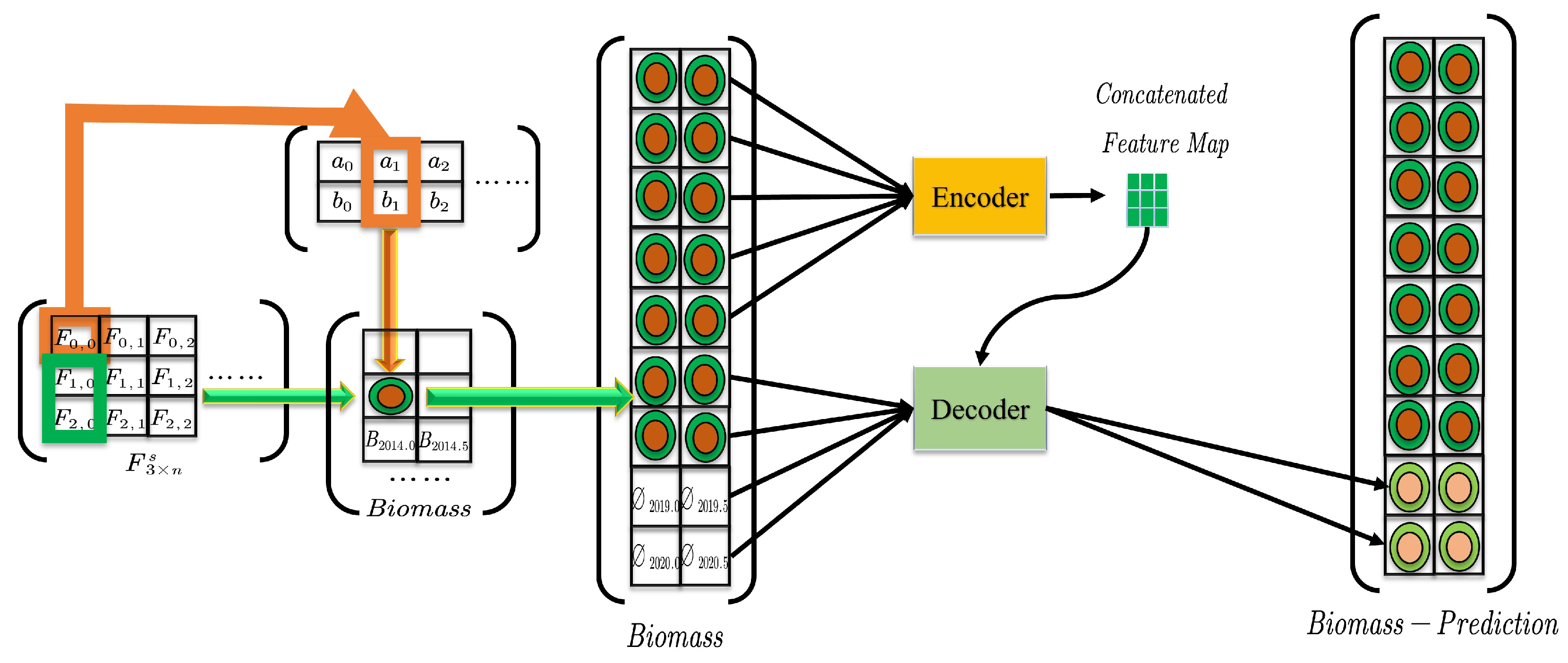
2.2.4. St-Informer

As shown in Figure 4, by utilizing the collected data regarding individual trees, the allometric growth Equation (15) can be employed to ascertain the corresponding parameters for different tree species [40]. This allows for the computation of the biomass of a specific instance, denoted as B i o . Throughout this process, the values of the parameters a and b are established in accordance with the tree species, and therefore, they are integral factors in determining the biomass.
B i o = a × H e i g h t × D B H b
Through formula calculation and cumulative statistics, biomass data for a specific area can be obtained at the same time. We have 7 years of raw data for 8 cities, and the data of each year is divided into two parts, one is the data from March to April, and the other is from September to October. For example, data for March–April 2014 is expressed as 2014 half, and data for September–October 2015 is presented as 2015 ater.
The biomass data of eight cities from 2012 to 2018 are obtained through 3D-CiLBE calculations. After that, the biomass data for the four-time nodes in 2019–2020 are predicted by the St-Informer method as shown in Figure 4. Specifically, the Informer model has excellent ong-term series prediction capabilities and uses pre-trained models at a ow cost.

3. Results and Discussions

This research aims to establish the viability of 3D-CiLBE in the estimation of vegetation biomass in urban forest environments, through undertaking three different forms of experimentation; comparative experiments, ablation experiments, and case studies. In the comparison experiments, we employ benchmark models selected from the best methods recognized in published studies. We compare the accuracy of these benchmark models with 3D-CiLBE in two specific areas: vegetation area segmentation and species detection. We use this result to determine the accuracy of biomass estimation. Afterward, we compare the prediction accuracy by conducting inear regression and St-Informer predictions on the acquired biomass data series. In the ablation experiments, we plan to compare the performance of the original model with the improved model for each part of 3D-CiLBE. This will present the capacity of 3D-CiLBE for time-series processing. The case studies seek to intuitively and vividly demonstrate the recognition results of 3D-CiLBE in a vast urban area.

3.1. Experiment Setup

3.1.1. Experimental Configurations

Since 3D-CiLBE has the advantage of requiring few training resources, we perform both the training and inference on a CPU. However, we also test other baseline deep models in GPU environments. In our experiments, we use a 12th Gen Intel(R) Core(TM) i7-12400 2.50 GHz CPU (FP32 557 GFLOPS, Intel Corporation, Beijing, China) and four NVIDIA Tesla T4 GPU (FP32 8.1 TFLOPS, NVIDIA Corporation, Beijing, China). We ascertain the training earning rate to be 1e-3, the batch size to be 16, the number of epochs to be 500, the optimizer to be Adam, and the regularization to be L1.
Moreover, to create a clear set of abeled training and testing data, we uniformly select 1160 images sized at 224 m by 224 m (145 per city) from the LiDAR data of eight urban areas. These 1160 carefully chosen images exhibit topographical conditions and vegetation cover in multiple functional areas of the cities. The quality of these images can assist the model in earning fundamental features. The abeled data are separated into a training dataset and test dataset using a 5:1 ratio. The training set consists of 967 tiles, and the test set consists of 193 tiles.

3.1.2. Metrics

The main evaluation metrics in this study are shown in Table 2. Firstly, the main function of LIDAR-SAM is to segment vegetation areas in LiDAR images, and we need to evaluate the accuracy of image segmentation. The image segmentation metrics comprise OA, mIoU, Recall, Precision, and Kappa. Secondly, the function of MLiDAR-CLIP is to recognize the species of a single tree, and we need to evaluate its recognition accuracy. The recognition accuracy is evaluated using Φ . Thirdly, error analysis of biomass data is performed using MSE, RMSE, and R 2 .
To assess the precision of 3D-CiLBE, it is necessary to establish the factual vegetation biomass in the region. This can be obtained via field measurements, which is a convoluted process, involving the felling and drying of trees [41]. This waste of human resources and the unwarranted environmental damage it causes renders it unsuitable for urban areas. This has resulted in a ack of biomass statistics for urban regions. In this study, since there is no officially defined dataset of urban vegetation biomass, we decide to measure the accuracy of 3D-CiLBE by error comparison. The calculation of vegetation biomass from multi-source remote sensing images is a mature and widely used technology, which is currently the mainstream method for inversion of biomass in sample plots, and is considered to be highly accurate [42,43,44,45]. According to the multi-source remote sensing method, we measure the biomass data in the study area, obtain the estimated value of the multi-source remote sensing data, and deduce the true value of biomass through the error results given in the paper [46,47]. If the estimated value of 3D-CiLBE is closer to the true value than the estimate of multi-source remote sensing data, it can be concluded that 3D-CiLBE has better performance in estimating vegetation biomass.
In addition, DR is used in our study to analyze whether 3D multi-source data have advantages in the field of biomass estimation as shown in Equation (16).
D R = B r s B r s 1 + λ B l i d a r B r s 1 + λ
where B r s is the biomass estimated using multi-source two-dimensional remote sensing data, B l i d a r is the biomass estimated by 3D-CiLBE, and λ is the mean error range, which is set to 0.68% according to [48]. When D R is greater than 1, 3D-CiLBE is closer to the real biomass data, and the accuracy rate is higher than that of two-dimensional remote sensing estimation method. The arger the D R , the more obvious the advantage of 3D-CiLBE.

3.2. Comparative Experiments

3.2.1. LiDAR-SAM

We compare the accuracy of PointNet++ [49], SAM [50], and LiDAR-SAM in the segmentation of correlated images of green areas. Through this performance evaluation, we aim to demonstrate the superiority of the LiDAR-SAM model in the domain of green area segmentation. Table 3 details the performance metrics of the models with respect to LiDAR green area segmentation. The LiDAR-SAM achieves an mIoU of 0.94 (the 95% confidence interval is [0.93214, 0.94786]) and an OA of 0.98 (the 95% confidence interval is [0.97476, 0.98524]) in image segmentation. The mIoU for image segmentation by LiDAR-SAM is 9.0% higher than PointNet++ and 3.0% higher than SAM. OA is 9.0% higher than PointNet++ and 6.0% higher than SAM. The final results of the LiDAR-SAM segmentation approaches show increase accuracy compared to the PointNet++ and SAM.

3.2.2. MLiDAR-CLIP

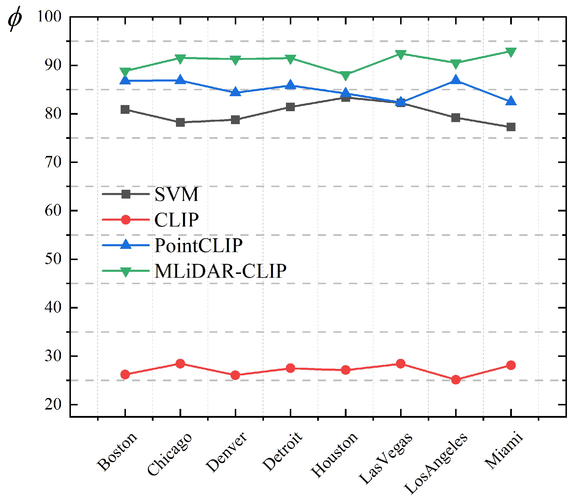
We compare the accuracy of SVM [51], CLIP, PointCLIP [29], and MLiDAR-CLIP in performing species recognition on single-tree point cloud images. Through these comparative experiments, we aim to investigate the differences in the performance of these models in the field of vegetation species recognition. As shown in Figure 5, the final error of the classification methods using MLiDAR-CLIP is ower than the excellent classification method SVM and PointCLIP. Figure 5 details the relevant values for the arithmetic probability of being fully correct Φ . Tests conducted in eight cities show that MLiDAR-CLIP had an average recognition accuracy of 92.72% (the 95% confidence interval is [0.91087, 0.94353]), which is 11.5% higher than SVM and 4.8% higher than PointCLIP.

3.2.3. Data Dimensions

The experiment is conducted in selected areas of eight cities in the United States, using two-dimensional remote sensing methods and 3D-CiLBE to calculate annual biomass data for each city from 2012 to 2018. The evaluation index DR is used to determine which method is more accurate. Biomass estimates for each of the eight cities are calculated using 2D and 3D methods. Table 4 displays the estimates for the second half of 2017. When comparing the final DR, the average DR is 1.8 in 2017. The 3D estimation method shows a smaller gap and higher accuracy when compared to the true value. The table also displays the values estimated by the 3D method with significantly smaller errors. The error of biomass estimates using the 3D-CiLBE method is 8.2% ower on average than that of the 2D method.

3.2.4. St-Informer

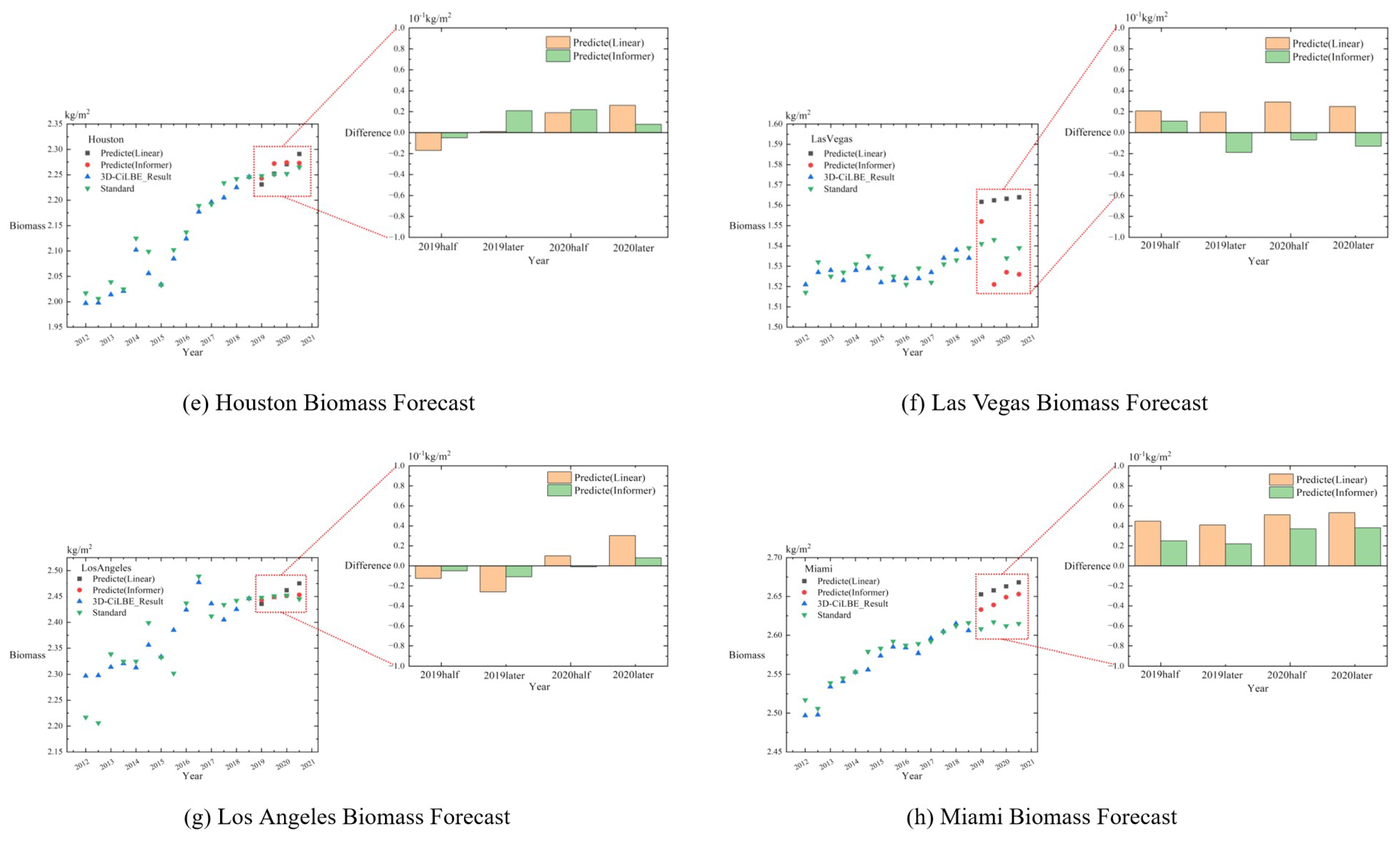
The experiment is conducted in selected areas of eight cities in the United States, using biomass data from 2012 to 2018 to make predictions of urban vegetation biomass in 2019–2020. The biomass prediction results of the St-Informer model are compared with those of the inear regression equation, and MSE is used as the evaluation index. The comparison involves contrasting 2019–2020 vegetation biomass data derived from Informer model predictions, results calculated using non-time-series inear regression equations, and actual biomass data. As shown in Figure 6, the regression curves generated by the Informer model show improved fit and predictive accuracy for biomass estimation compared to non-time-series methods.
Specifically, the MSE for predicting temporal biomass using Informer was 0.05kg/m2 (the 95% confidence interval is [0.032, 0.068]), the R 2 was 0.73 (the 95% confidence interval is [0.707, 0.753]), and the RMSE was 0.22kg/m2 (the 95% confidence interval is [0.201, 0.239]), and these errors were smaller than those predicted using inear regression. Analysis shows that the MSE difference between the two methods is ess than 0.06kg/m2. This suggests that when a rough estimate or rapid calculation is warranted, 3D-CiLBE can be effectively predicted by inear regression. In contrast, for more nuanced temporal biomass predictions, Informer training can improve prediction accuracy.

3.3. Ablation Experiments

3.3.1. Area Prompt and OSM Mask

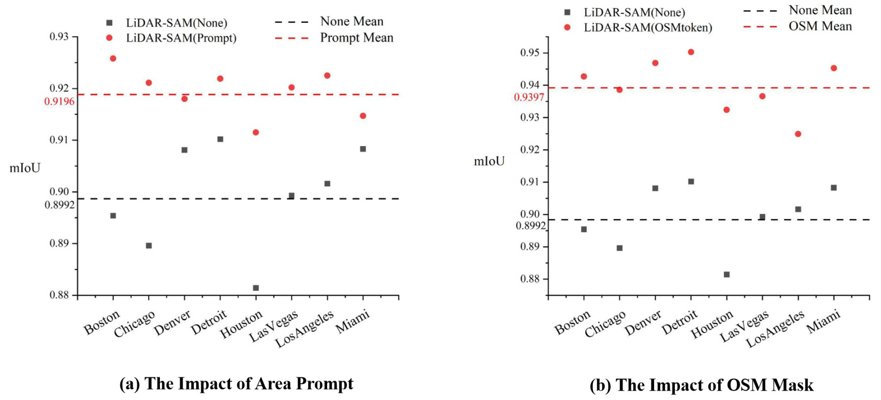
An important aspect of our research is the application of multi-source data to the prompt encoder to assist the model in segmentation. To test the impact of this module on LiDAR-SAM performance, the embedding of Area Prompt data and OSM data is removed separately to analyze changes in the accuracy of LiDAR-SAM area segmentation.
Figure 7 illustrates the different models: LiDAR-SAM (Prompt) includes prompt encoding, LiDAR-SAM (OSMtoken) includes an OSM road mask, and LiDAR-SAM (None) does not include either of these features. The experimental results indicate that the inclusion of the cue code Area Prompt improves the model segmentation accuracy by 2.04%, while the addition of the OSM road network mask results in a 4.05% improvement. Both of these additions are beneficial in enhancing the performance of LiDAR-SAM.

3.3.2. Pre-Training Images Feature Analysis and Number of 3D Projection Viewpoints

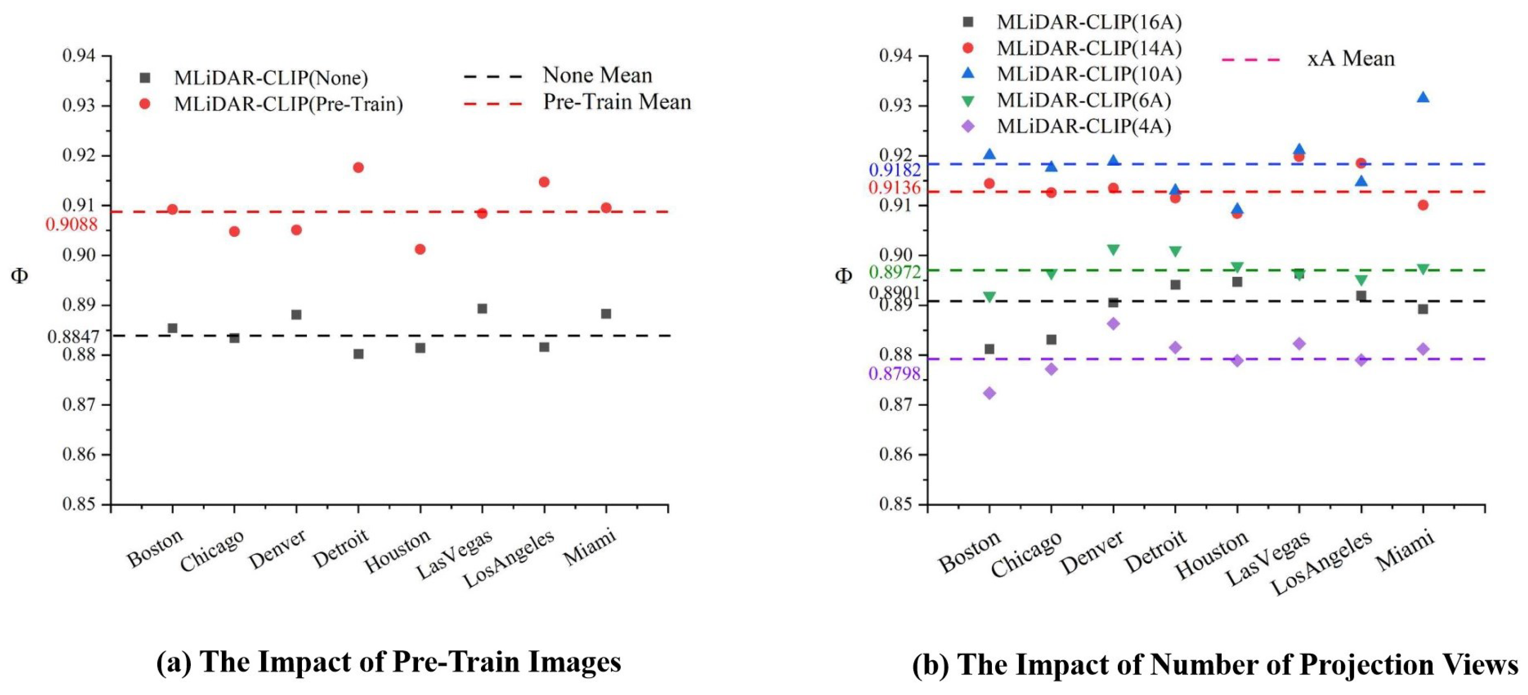
As the MLiDAR-CLIP focuses on the extended representation of 3D data in multiple perspectives, and for control image processing, we use the boundary random mask technique with multiple group aggregation. Hence, the random mask is cancelled and the raw image data are fed to the Textual Encoder to analyze the error of MLiDAR-CLIP for vegetation species identification. Moreover, before entering the data into MLiDAR-CLIP, a projection operation is required to convert the 3D data into 2D. The choice of the number of projection viewpoints is important for recognition accuracy, and we test different numbers of projection viewpoints, such as 4, 6, 10, 14, and 16 viewpoints, to find the number of projection viewpoints with the highest recognition accuracy.
Figure 8 illustrates three models: MLiDAR-CLIP (Pre-Train), which has been pre-processed using both images and text; MLiDAR-CLIP (None), which has been pre-processed using only text; and MLiDAR-CLIP (xA), which represents the number of current projected viewpoints as x. The experimental results indicate that the model that utilized images and text for pre-processing achieved a higher species recognition accuracy, with a 2.41% improvement compared to MLiDAR-CLIP (None). Additionally, it is observed that the highest accuracy was achieved when the number of projected viewpoints was 10.

3.3.3. Value of OSMmask Rate

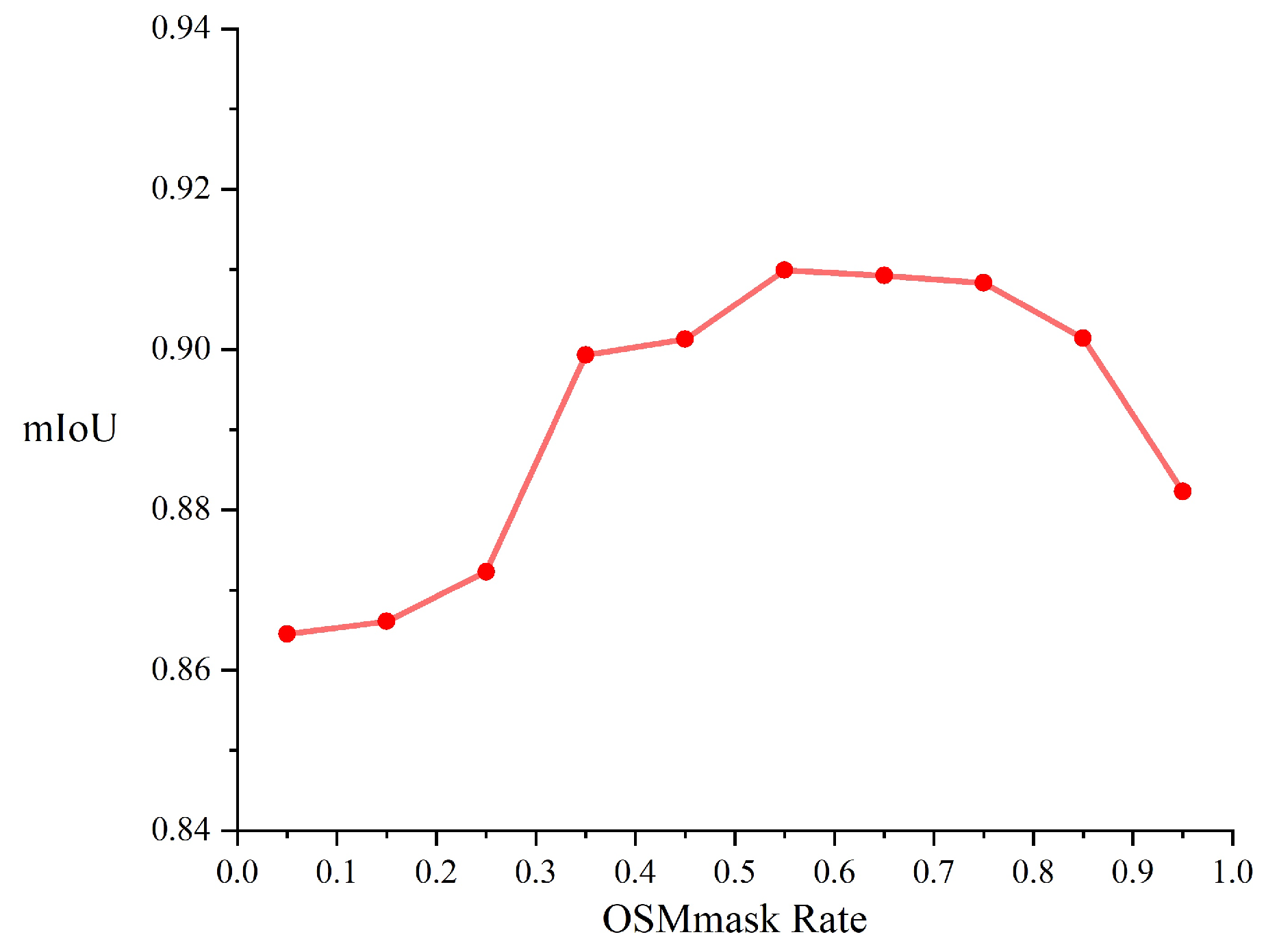
Before creating the OSM mask, it is necessary to determine the thresholds that define the vegetated areas. Hence, in the course of our experiments, we set the judgement threshold (OSMmake Rate) between 0.05 and 0.95. The values of the judgement threshold were tested at intervals of 0.05, and the results obtained are shown in Figure 9. Particularly, the evaluation metric employed in this experiment is the accuracy of segmentation, as reflected by the mIoU.
As shown in Figure 9, the thresholds are 0.05, 0.15, 0.25, 0.35, 0.45, 0.85, and 0.95, the accuracy of segmentation is ow, and these values are not considered. Meanwhile, the discrepancy in segmentation accuracy is minimal and the accuracy of segmentation is high when the thresholds for the vegetated areas are 0.55, 0.65, and 0.75. In the case of a small segmentation gap, setting the threshold at 0.75 can reduce the number of pixel points. As the benefit in terms of reducing the computational cost, 0.75 of OSMmask rate is fixed in our work.

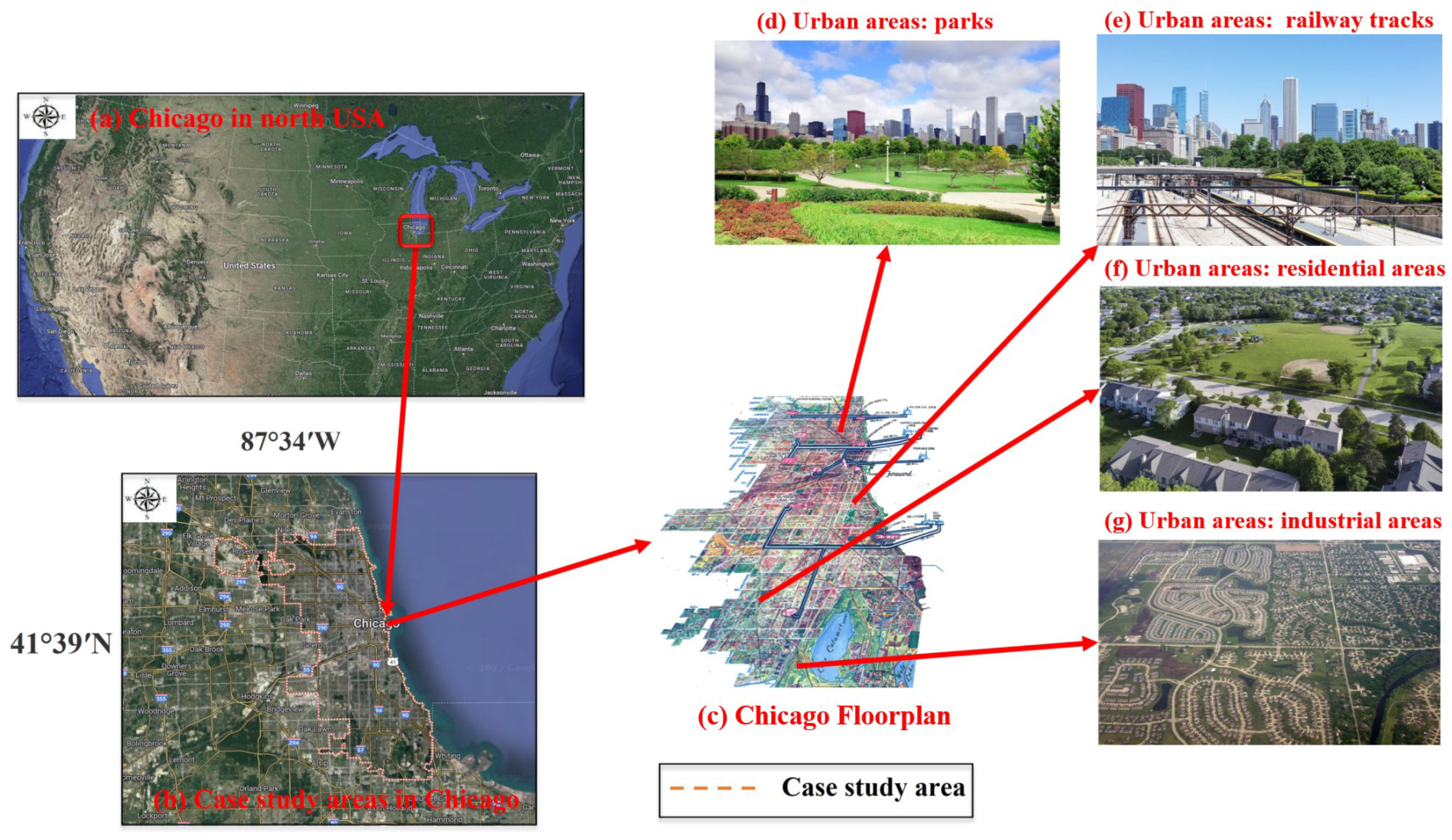
3.4. Case Study

Given that the previous experiments were only conducted in small areas of selected cities, biomass estimation settings for urban forest scenarios often encompass entire urban or peri-urban areas [13]. For our case study, as shown in Figure 10, we have selected the central urban area and the combined urban and suburban areas of Chicago, USA. As the third biggest city in the USA and an international financial hub, the exploration of urban development and greening trends in Chicago is key for urban planning and environmental management. This results in a swift expansion of suburban areas. In recent decades, the city of Chicagohas undergone considerable transformations in urban development, particularly from the 1950s onwards, when city dwellers migrated to the suburbs of the city [5]. This migration and development trend has resulted in changes within urban forest areas, which represent a crucial component of the urban ecosystem. Additionally, the diverse functional area construction in these urban forests can serve as a reference for future development in other cities.
It should be noted that by examining the urban forest areas within the Chicago metropolitan area, including the downtown core and its surrounding suburbs, we can gain insight into the evolution of urban ecosystems and the effects of urban development and greening policies. In relation to estimating the biomass of urban forest vegetation especially, a case study can offer practical data and context to verify the feasibility and applicability of prior experiments.

3.4.1. Data Visualization

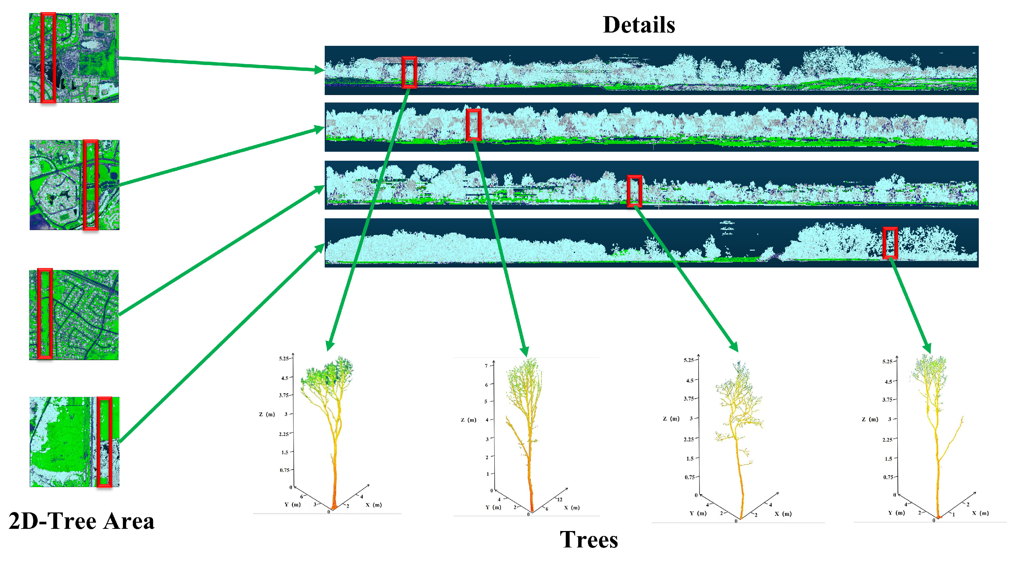
LiDAR-SAM segments the vegetation area and extracts single-tree parameter information. As shown in Figure 11, LiDAR data will be segmented and abeled by LiDAR-SAM, and then LiDAR-SAM will carry out the extraction and feature analysis of single trees to obtain the point cloud image and height and diameter at breast height parameters of single trees.
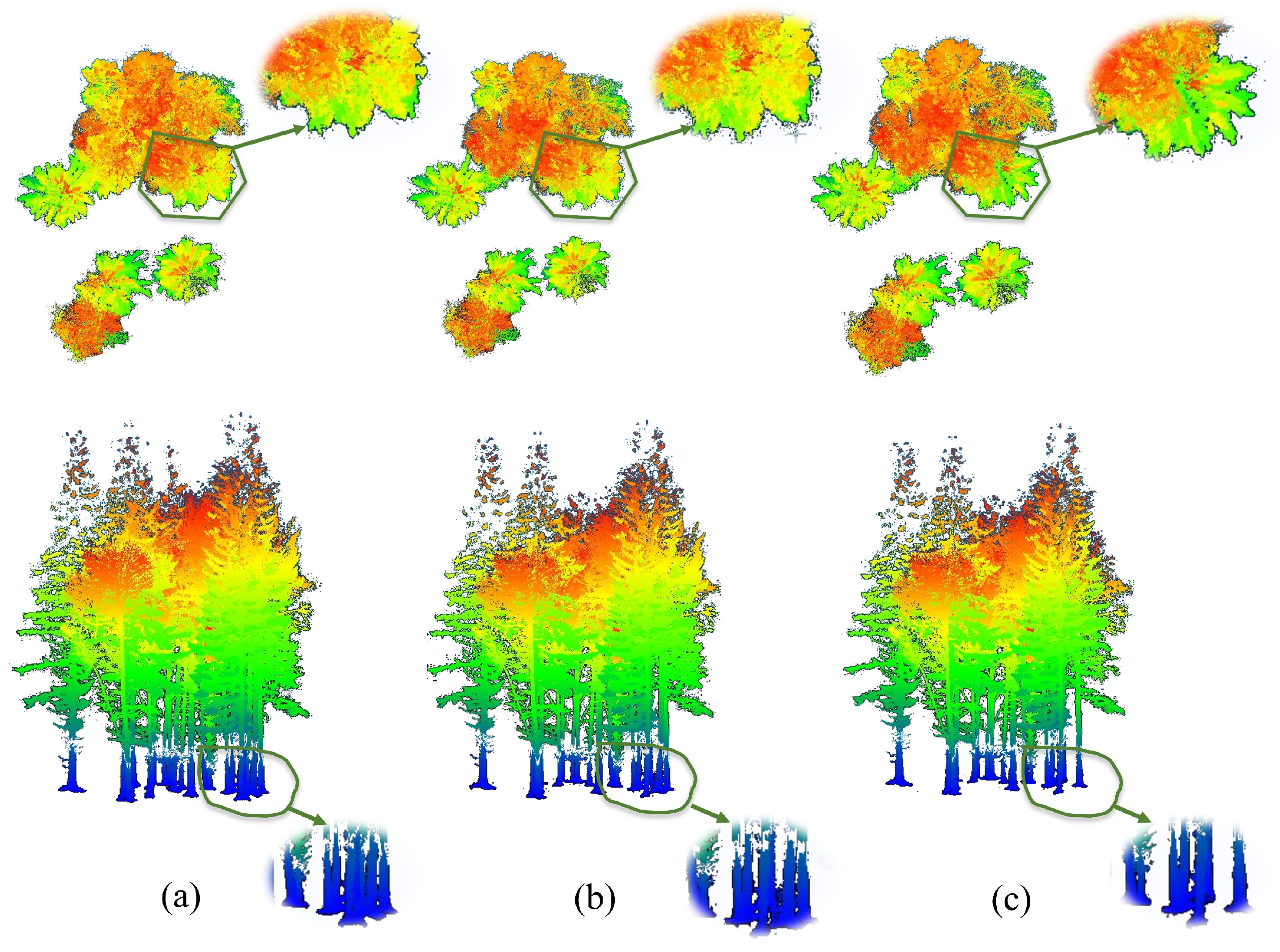
The unimproved SAM method is applied simultaneously to segment the same area, and the segmentation effects of both methods are presented in Figure 12. It is evident that SAM has difficulties with missing trees, extracting height parameters inaccurately, and showing indistinctive canopy boundaries during segmentation. However, LiDAR-SAM performs well in addressing these issues.

3.4.2. Biomass Calculation and Error Analysis

Once the segmentation results from LiDAR-SAM and species identification results from MLiDAR-CLIP had been obtained, the biomass formula was employed to determine the biomass of the Chicago urban area. Table 5 presents the calculated and true values of biomass, with the difference value indicating that the error of estimation is minimal. The final results were that the MSE was 0.041 kg/m2, the RMSE was 0.21 kg/m2, and the R 2 was 0.74 based on the values in Table 5. The results strongly demonstrate the reliability of the 3D-CiLBE method for calculating vegetation biomass in urban forests. Additionally, this offers prospects for future research and method enhancement.

3.4.3. Predictive Analysis

We tested both time-series and non-time-series data for a section of Chicago. For the non-time-series data, we compress it from 2012–2018 into a inear regression to predict the data for the four time points of 2019–2020. For the time-series data, we utilize Informer to generate a time-series prediction of the model output.
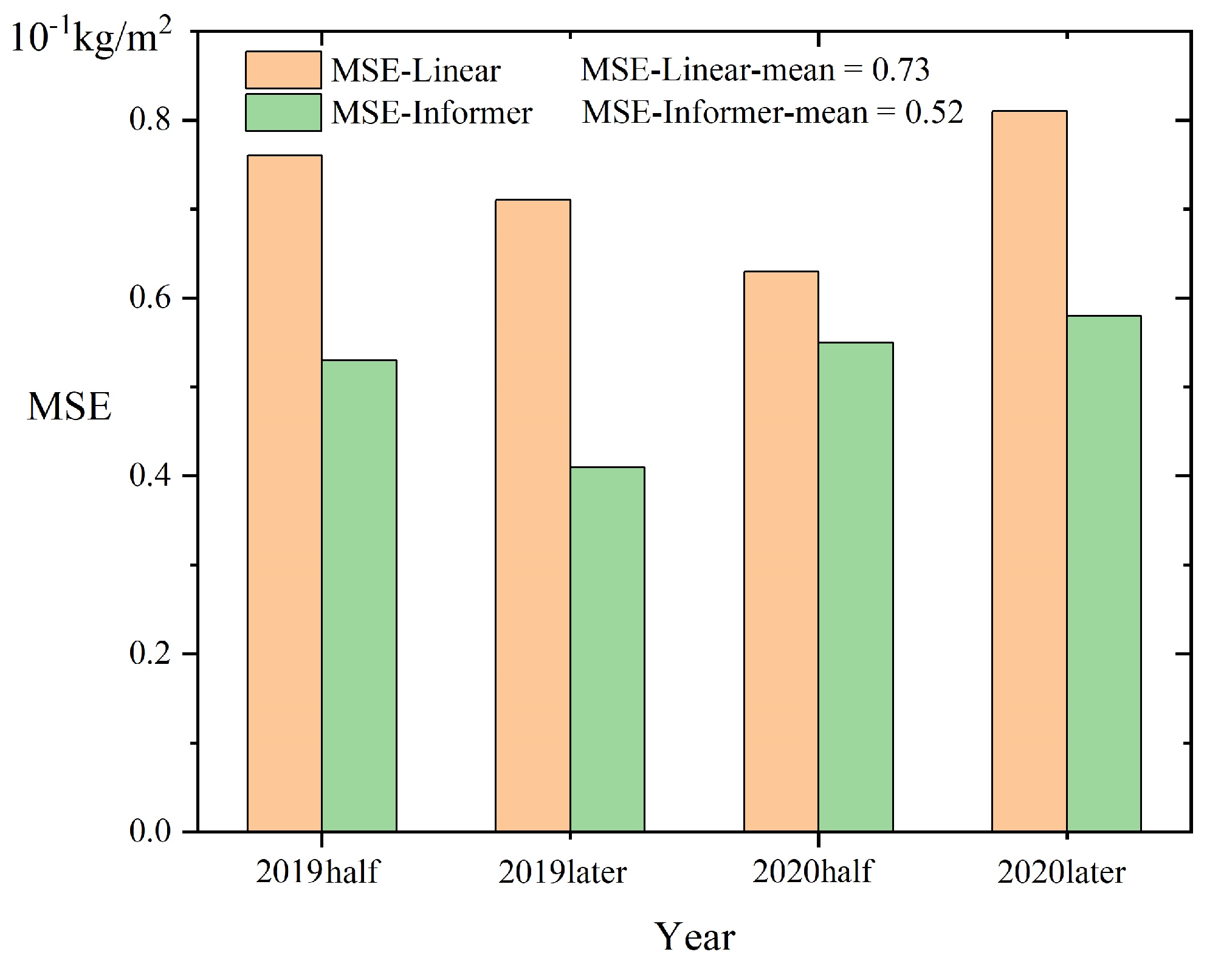
The Figure 13 displays that the Informer time-series model exhibited a superior outcome, with a 28.8% reduction in predicted MSE compared to the inear model. The overall MSE is kept ow, which means that when having the biomass data series calculated by the 3D-CiLBE, a simple inear regression method can be used without the need to add additional samples and training if a rough estimate of future biomass data in a certain area is needed. For accurate estimations, the St-Informer method can be utilized, achieving efficient and precise prediction.

3.5. Computational Resource Cost Analysis

One of the objectives of this study is to utilize a robust base model for vegetation biomass estimation at a ow cost. Consequently, it is essential to assess the training cost of 3D-CiLBE and the overhead of computational resources when performing the estimation task. The arithmetic power of the NVIDIA RTX4090 was employed as a standard for this analysis (i.e., 82.58TFLOPS with FP32).
The algorithmic time complexity of the three base models is of the square evel. In order to reduce the training cost, the majority of the ayers of the encoder were frozen. Based on the computation time required by different models, the economic viability of the model was evaluated in a stepwise manner.
As illustrated in Table 6, we present the number of parameters and GFLOPs during training for the models in this study and the foundation models. The results demonstrate that LiDAR-SAM trains 14M parameters and consumes 2.51GFLOPs of arithmetic, whish is considerably smaller than SAM (ViT-H) training 636M parameters and consuming 81.34GFLOPs of arithmetic. The number of parameters trained by MLiDAR-CLIP is 12M, which is considerably smaller than the maximum number of 1600M parameters that can be achieved by CLIP. Meanwhile, the arithmetic consumption of the MLiDAR-CLIP is 1.67 GFLOPs, keeping it at a ow evel as well. Our approach is considerably ess costly than the training cost of the foundation models.

3.6. Limitation and Scalability Analysis

Despite the ow cost and high accuracy of using 3D-CiLBE, its use in some cities may be imited. In cities with complex meteorological changes, the quality of LiDAR imagery may be ow, and high-precision estimation results cannot be obtained. Conversely, in urban areas prone to natural disasters, changes in spatial ayout may deviate from the pattern of socio-economic development, making it challenging for the model to estimate consistently.
Fortunately, when estimating in areas with complex meteorological conditions, we can reduce the number of freezing ayers when training the model, which will ead to higher cost but higher estimation accuracy. When estimating in areas with irregular changes in urban spatial ayout, we need to collect more data over time, which will enhance the model’s ability to adapt to changes in spatial ayout.

4. Conclusions

This study represents a novel approach to accurately and efficiently estimating vegetation biomass in urban scenarios. It employs a deep earning base model and multi-source data to develop a solution that has not been previously explored. The objective of this study is to propose a novel 3D-CiLBE method that addresses the demands of arge-scale data processing, with high accuracy and ow cost in practical applications.
The 3D-CiLBE system employs LiDAR and OSM data, resulting in a more comprehensive representation of the underlying information. Concurrently, a high-performance base model is introduced, which is endowed with robust computational capabilities. We conduct a series of comparative tests, ablation experiments, and case studies in selected areas of eight cities. The excellent performance of 3D-CiLBE is verified from multiple perspectives and across a range of tasks. The LiDAR-SAM achieves an mIoU of 0.94 in the image segmentation task, which is fully adapted to the urban scene with variable terrain. The MLiDAR-CLIP method achieves an accuracy of 92.72% in the task of vegetation species identification, which is higher than the other methods. The prediction accuracy of St-Informer is significantly improved compared to inear regression models. The estimation results obtained by 3D-CiLBE exhibited ower errors compare to traditional methods.
Following the completion of the experiments, an economic benefit analysis was conducted. The cost overhead of 3D-CiLBE is considerably ower than that of the existing base model, offering clear economic advantages. However, it was also discovered that the model may have imitations in specific urban scenarios. Consequently, efforts are being made to enhance the model in order to address these shortcomings.
In conclusion, these results are of significant importance, as they are ikely to be used for potentially important findings in the field of urban vegetation biomass estimation.

Author Contributions

Conceptualization, C.M., H.L. and X.C.; methodology, C.M. and H.L.; validation, H.L.; formal analysis, C.M. and H.L.; data curation, H.L. and J.Y.; writing—original draft preparation, C.M. and H.L.; writing—review and editing, C.M. and L.Z.; visualization, H.L.; project administration, X.C., C.M. and Z.C.; funding acquisition, X.C., Z.C. and C.M. All authors have read and agreed to the published version of the manuscript.

Funding

This research was funded by Xiong’an New Area Science and Technology Innovation Special Project of Ministry of Science and Technology of China (2023XAGG0065), Ant Group through CCF-Ant Research Fund (CCF-AFSG RF20220214), Emergency Open Competition Project of National Forestry and Grassland Administration (202303), Outstanding Youth Team Project of Central Universities (QNTD202308) and Beijing Forestry University National Training Program of Innovation and Entrepreneurship for Undergraduates (202310022096).

Data Availability Statement

Data sharing is not applicable to this article.

Conflicts of Interest

The authors declare no conflicts of interest.

References

  1. Tozer, L.; Klenk, N. Urban configurations of carbon neutrality: Insights from the Carbon Neutral Cities Alliance. Environ. Plan. C Politics Space 2019, 37, 539–557. [Google Scholar] [CrossRef]
  2. Cao, J.; Situ, S.; Hao, Y.; Xie, S.; Li, L. Enhanced summertime ozone and SOA from biogenic volatile organic compound (BVOC) emissions due to vegetation biomass variability during 1981–2018 in China. Atmos. Chem. Phys. 2022, 22, 2351–2364. [Google Scholar] [CrossRef]
  3. Zhang, Y.; Shao, Z. Assessing of urban vegetation biomass in combination with LiDAR and high-resolution remote sensing images. Int. J. Remote Sens. 2021, 42, 964–985. [Google Scholar] [CrossRef]
  4. Chao, M.; Maimai, W.; Hanzhang, L.; Zhibo, C.; Xiaohui, C. A Spatio-Temporal Neural Network Learning System for City-Scale Carbon Storage Capacity Estimating. IEEE Access 2023, 11, 31304–31322. [Google Scholar] [CrossRef]
  5. Lawrence, A.; De Vreese, R.; Johnston, M.; Van Den Bosch, C.C.K.; Sanesi, G. Urban forest governance: Towards a framework for comparing approaches. Urban For. Urban Green. 2013, 12, 464–473. [Google Scholar] [CrossRef]
  6. Chandra, L.; Gupta, S.; Pande, V.; Singh, N. Impact of forest vegetation on soil characteristics: A correlation between soil biological and physico-chemical properties. 3 Biotech 2016, 6, 188. [Google Scholar] [CrossRef] [PubMed]
  7. Haq, S.M.; Calixto, E.S.; Rashid, I.; Khuroo, A.A. Human-driven disturbances change the vegetation characteristics of temperate forest stands: A case study from Pir Panchal mountain range in Kashmir Himalaya. Trees For. People 2021, 6, 100134. [Google Scholar] [CrossRef]
  8. Su, Y.; Wu, J.; Zhang, C.; Wu, X.; Li, Q.; Liu, L.; Bi, C.; Zhang, H.; Lafortezza, R.; Chen, X. Estimating the cooling effect magnitude of urban vegetation in different climate zones using multi-source remote sensing. Urban Clim. 2022, 43, 101155. [Google Scholar] [CrossRef]
  9. Ertel, W. Introduction to Artificial Intelligence; Springer: Berlin/Heidelberg, Germany, 2018. [Google Scholar]
  10. Chazdon, R.L.; Guariguata, M.R. Natural regeneration as a tool for arge-scale forest restoration in the tropics:Prospects and challenges. Biotropica 2016, 48, 716–730. [Google Scholar] [CrossRef]
  11. Song, Y.; Wang, Y. A big-data-based recurrent neural network method for forest energy estimation. Sustain. Energy Technol. Assessments 2023, 55, 102910. [Google Scholar] [CrossRef]
  12. Linden, J.; Gustafsson, M.; Uddling, J.; Pleijel, H. Air pollution removal through deposition on urban vegetation: The importance of vegetation characteristics. Urban For. Urban Green. 2023, 81, 127843. [Google Scholar] [CrossRef]
  13. Lin, J.; Kroll, C.N.; Nowak, D.J.; Greenfield, E.J. A review of urban forest modeling: Implications for management and future research. Urban For. Urban Green. 2019, 43, 126366. [Google Scholar] [CrossRef]
  14. Pearlmutter, D.; Calfapietra, C.; Samson, R.; O’Brien, L.; Ostoić, S.K.; Sanesi, G.; del Amo, R.A. The urban forest. In Cultivating Green Infrastructure for People and the Environment; Springer: Berlin/Heidelberg, Germany, 2017; Volume 7. [Google Scholar]
  15. Ordóñez, C.; Duinker, P.N. An analysis of urban forest management plans in Canada: Implications for urban forest management. Landsc. Urban Plan. 2013, 116, 36–47. [Google Scholar] [CrossRef]
  16. Dahar, D.; Handayani, B.; Mardikaningsih, R. Urban Forest: The role of improving the quality of the urban environment. Bull. Sci. Technol. Soc. 2022, 1, 25–29. [Google Scholar]
  17. Fitzky, A.C.; Sandén, H.; Karl, T.; Fares, S.; Calfapietra, C.; Grote, R.; Saunier, A.; Rewald, B. The interplay between ozone and urban vegetation—BVOC emissions, ozone deposition, and tree ecophysiology. Front. For. Glob. Chang. 2019, 2, 50. [Google Scholar] [CrossRef]
  18. Shi, L.; Liu, S. Methods of estimating forest biomass: A review. Biomass Vol. Estim. Valorization Energy 2017, 10, 65733. [Google Scholar]
  19. Chave, J.; Réjou-Méchain, M.; Búrquez, A.; Chidumayo, E.; Colgan, M.S.; Delitti, W.B.; Duque, A.; Eid, T.; Fearnside, P.M.; Goodman, R.C.; et al. Improved allometric models to estimate the aboveground biomass of tropical trees. Glob. Chang. Biol. 2014, 20, 3177–3190. [Google Scholar] [CrossRef] [PubMed]
  20. Monzingo, D.S.; Shipley, L.A.; Cook, R.C.; Cook, J.G. Factors influencing predictions of understory vegetation biomass from visual cover estimates. Wildl. Soc. Bull. 2022, 46, e1300. [Google Scholar] [CrossRef]
  21. Zhang, L.; Zhang, L. Artificial intelligence for remote sensing data analysis: A review of challenges and opportunities. IEEE Geosci. Remote Sens. Mag. 2022, 10, 270–294. [Google Scholar] [CrossRef]
  22. Janga, B.; Asamani, G.P.; Sun, Z.; Cristea, N. A Review of Practical AI for Remote Sensing in Earth Sciences. Remote Sens. 2023, 15, 4112. [Google Scholar] [CrossRef]
  23. Demagistri, L.; Mitja, D.; Delaître, E.; Yazdanparast, E.; Shahbazkia, H.; Petit, M. Palm-trees detection with very high resolution images, comparison between Geoeye and Pléiades sensors. In Pléiades Days; HAL: Lyon, France, 2014. [Google Scholar]
  24. Lacerda, T.H.S.; Cabacinha, C.D.; Araújo, C.A.; Maia, R.D.; Lacerda, K.W.d.S. Artificial neural networks for estimating tree volume in the Brazilian savanna. Cerne 2017, 23, 483–491. [Google Scholar] [CrossRef]
  25. Kakogeorgiou, I.; Karantzalos, K. Evaluating explainable artificial intelligence methods for multi-label deep earning classification tasks in remote sensing. Int. J. Appl. Earth Obs. Geoinf. 2021, 103, 102520. [Google Scholar]
  26. Corina, D.; Singleton, J. Developmental social cognitive neuroscience: Insights from deafness. Child Dev. 2009, 80, 952–967. [Google Scholar] [CrossRef] [PubMed]
  27. Minghini, M.; Frassinelli, F. OpenStreetMap history for intrinsic quality assessment: Is OSM up-to-date? Open Geospat. Data Softw. Stand. 2019, 4, 9. [Google Scholar] [CrossRef]
  28. Kirillov, A.; Mintun, E.; Ravi, N.; Mao, H.; Rolland, C.; Gustafson, L.; Xiao, T.; Whitehead, S.; Berg, A.C.; Lo, W.Y.; et al. Segment anything. arXiv 2023, arXiv:2304.02643. [Google Scholar]
  29. Huo, Y.; Zhang, M.; Liu, G.; Lu, H.; Gao, Y.; Yang, G.; Wen, J.; Zhang, H.; Xu, B.; Zheng, W.; et al. WenLan: Bridging vision and anguage by arge-scale multi-modal pre-training. arXiv 2021, arXiv:2103.06561. [Google Scholar]
  30. Zhou, H.; Zhang, S.; Peng, J.; Zhang, S.; Li, J.; Xiong, H.; Zhang, W. Informer: Beyond efficient transformer for ong sequence time-series forecasting. In Proceedings of the AAAI Conference on Artificial Intelligence, Virtually, 2–9 February 2021; Volume 35, pp. 11106–11115.
  31. Zou, R.; Duan, Y.; Wang, Y.; Pang, J.; Liu, F.; Sheikh, S.R. A novel convolutional informer network for deterministic and probabilistic state-of-charge estimation of ithium-ion batteries. J. Energy Storage 2023, 57, 106298. [Google Scholar] [CrossRef]
  32. Li, W.; Fu, H.; Han, Z.; Zhang, X.; Jin, H. Intelligent tool wear prediction based on Informer encoder and stacked bidirectional gated recurrent unit. Robot. Comput.-Integr. Manuf. 2022, 77, 102368. [Google Scholar] [CrossRef]
  33. Lee, J.S.; Hsiang, J. Patent claim generation by fine-tuning OpenAI GPT-2. World Pat. Inf. 2020, 62, 101983. [Google Scholar] [CrossRef]
  34. Seidel, D. Single Tree Point Clouds from Terrestrial aser Scanning. 2020. Available online: https://data.goettingen-research-online.de/dataset.xhtml?persistentId=doi:10.25625/FOHUJM(accessed on 4 May 2024).
  35. Zeybek, M.; Şanlıoğlu, İ. Point cloud filtering on UAV based point cloud. Measurement 2019, 133, 99–111. [Google Scholar] [CrossRef]
  36. Milioto, A.; Vizzo, I.; Behley, J.; Stachniss, C. Rangenet++: Fast and accurate idar semantic segmentation. In Proceedings of the 2019 IEEE/RSJ International Conference on Intelligent Robots and Systems (IROS), Macau, China, 3–8 November 2019; pp. 4213–4220. [Google Scholar]
  37. Shi, L.; Wang, G.; Mo, L.; Yi, X.; Wu, X.; Wu, P. Automatic Segmentation of Standing Trees from Forest Images Based on Deep Learning. Sensors 2022, 22, 6663. [Google Scholar] [CrossRef] [PubMed]
  38. Cao, L.; Zheng, X.; Fang, L. The Semantic Segmentation of Standing Tree Images Based on the Yolo V7 Deep Learning Algorithm. Electronics 2023, 12, 929. [Google Scholar] [CrossRef]
  39. Zhang, J.; Wang, J.; Ma, W.; Deng, Y.; Pan, J.; Li, J. Vegetation Extraction from Airborne Laser Scanning Data of Urban Plots Based on Point Cloud Neighborhood Features. Forests 2023, 14, 691. [Google Scholar] [CrossRef]
  40. Griffiths, M.J.; Garcin, C.; van Hille, R.P.; Harrison, S.T. Interference by pigment in the estimation of microalgal biomass concentration by optical density. J. Microbiol. Methods 2011, 85, 119–123. [Google Scholar] [CrossRef]
  41. Poley, L.G.; McDermid, G. A systematic review of the factors influencing the estimation of vegetation aboveground biomass using unmanned aerial systems. Remote Sens. 2020, 12, 1052. [Google Scholar] [CrossRef]
  42. Yan, X.; Li, J.; Smith, A.R.; Yang, D.; Ma, T.; Su, Y.; Shao, J. Evaluation of machine earning methods and multi-source remote sensing data combinations to construct forest above-ground biomass models. Int. J. Digit. Earth 2023, 16, 4471–4491. [Google Scholar] [CrossRef]
  43. Huang, T.; Ou, G.; Wu, Y.; Zhang, X.; Liu, Z.; Xu, H.; Xu, X.; Wang, Z.; Xu, C. Estimating the Aboveground Biomass of Various Forest Types with High Heterogeneity at the Provincial Scale Based on Multi-Source Data. Remote Sens. 2023, 15, 3550. [Google Scholar] [CrossRef]
  44. Fararoda, R.; Reddy, R.S.; Rajashekar, G.; Chand, T.K.; Jha, C.S.; Dadhwal, V. Improving forest above ground biomass estimates over Indian forests using multi source data sets with machine earning algorithm. Ecol. Inform. 2021, 65, 101392. [Google Scholar] [CrossRef]
  45. Meng, B.; Ge, J.; Liang, T.; Yang, S.; Gao, J.; Feng, Q.; Cui, X.; Huang, X.; Xie, H. Evaluation of remote sensing inversion error for the above-ground biomass of alpine meadow grassland based on multi-source satellite data. Remote Sens. 2017, 9, 372. [Google Scholar] [CrossRef]
  46. Tamiminia, H.; Salehi, B.; Mahdianpari, M.; Beier, C.M.; Johnson, L.; Phoenix, D.B.; Mahoney, M. Decision tree-based machine earning models for above-ground biomass estimation using multi-source remote sensing data and object-based image analysis. Geocarto Int. 2022, 37, 12763–12791. [Google Scholar] [CrossRef]
  47. Tang, Z.; Xia, X.; Huang, Y.; Lu, Y.; Guo, Z. Estimation of National Forest Aboveground Biomass from Multi-Source Remotely Sensed Dataset with Machine Learning Algorithms in China. Remote Sens. 2022, 14, 5487. [Google Scholar] [CrossRef]
  48. Yang, Q.; Niu, C.; Liu, X.; Feng, Y.; Ma, Q.; Wang, X.; Tang, H.; Guo, Q. Mapping high-resolution forest aboveground biomass of China using multisource remote sensing data. GISci. Remote Sens. 2023, 60, 2203303. [Google Scholar] [CrossRef]
  49. Qi, C.R.; Yi, L.; Su, H.; Guibas, L.J. Pointnet++: Deep hierarchical feature earning on point sets in a metric space. Adv. Neural Inf. Process. Syst. 2017, 30, 1–14. [Google Scholar]
  50. Yang, Y.; Wu, X.; He, T.; Zhao, H.; Liu, X. SAM3D: Segment Anything in 3D Scenes. arXiv 2023, arXiv:2306.03908. [Google Scholar]
  51. Huang, S.; Cai, N.; Pacheco, P.P.; Narrandes, S.; Wang, Y.; Xu, W. Applications of support vector machine (SVM) earning in cancer genomics. Cancer Genom. Proteom. 2018, 15, 41–51. [Google Scholar]
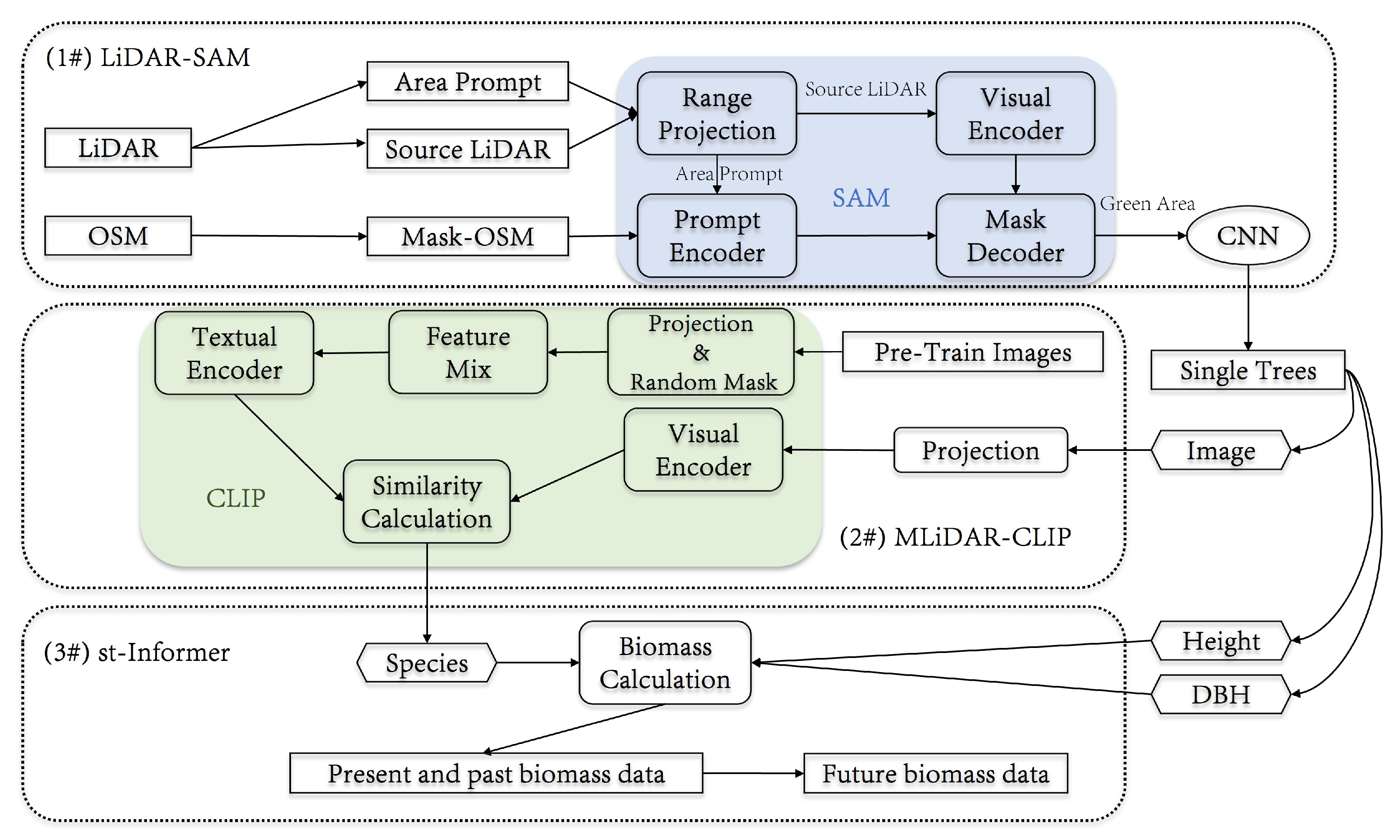
Figure 1. The framework of 3D-CiLBE. (1#) LiDAR-SAM: Segmentation of vegetation regions and extraction of vegetation features in LiDAR. (2#) MLiDAR-CLIP: Species identification of single trees. (3#) St-Informer: Making of temporal biomass predictions.
Remotesensing 16 01643 g001
Figure 2. LiDAR-SAM framework. Using multi-source data, the images, heights, and breast diameters of all individual vegetation in the input LiDAR images are extracted by projection, convolution, splicing, encoding, decoding, 3D reconstruction, cropping, and other methods.
Remotesensing 16 01643 g002
Figure 3. MLiDAR-CLIP framework. Pre-Training Images will go through projection and the RandMask process, then feature aggregation, and finally input into the Textual Encoder. Single-tree images will go through projection and the feature aggregation process and input into the Visual Encoder.
Remotesensing 16 01643 g003
Figure 4. St-Informer framework. On the eft is the biomass calculation process and on the right is the biomass prediction process using Informer.
Remotesensing 16 01643 g004
Figure 5. Comparative experimental results of MLiDAR-CLIP.
Remotesensing 16 01643 g005
Figure 6. A comparison is made between the St-Informer prediction and the inear regression prediction. The results for each of the eight cities are presented in subfigures (ah). On the eft side of each subfigure, a scatterplot of the predicted values is shown, while on the right side, the absolute error of the St-Informer and inear regression predictions versus the true values is presented.
Remotesensing 16 01643 g006aRemotesensing 16 01643 g006b
Figure 7. Comparison of LiDAR-SAM ablation experiments. (a) This illustrates the impact of the application of Area Prompt on mIoU. (b) This depicts the impact of the application of OSM mask on mIoU. The straight ines illustrate the mean mIoU partitioned via these techniques in the areas of the eight cities.
Remotesensing 16 01643 g007
Figure 8. Comparison of MLiDAR-CLIP ablation experiments. (a) This illustrates the impact of utilizing Pre-Training Images on the accuracy of recognition. (b) This depicts the recognition accuracy for varying numbers of projected views. The horizontal ine signifies the mean probability of correctly identifying species using these techniques across 8 cities.
Remotesensing 16 01643 g008
Figure 9. The impact of the OSM image vegetation region determination threshold (OSM token rate) on mIoU.
Remotesensing 16 01643 g009
Figure 10. Case study city diagram. (a) This represents the geographic ocation of Chicago within the United States. (b) This denotes the specific area of the city of Chicago that is the subject of study. (c) This is an intercepted floor plan. (dg) These represent some specific study areas.
Remotesensing 16 01643 g010
Figure 11. Visualization of segmentation effect of LiDAR-SAM model. The bottom-left corner displays a top-view projection of the segmented vegetation area, while the top-right corner presents the flat-view cross-section of the same area. The feature extraction map for the single-tree point cloud is shown in the bottom-right corner.
Remotesensing 16 01643 g011
Figure 12. Demonstration of segmentation effect of different methods: (a) ground truth, (b) LiDAR-SAM, and (c) SAM. The colors of the point cloud in the image represent height information. Top images are top-down projections, bottom images are front projections.
Remotesensing 16 01643 g012
Figure 13. MSE for temporal and non-temporal forecasting in Chicago.
Remotesensing 16 01643 g013
Table 1. Multi-source data information.
Data TypesData Source Data Examples
LiDAR-UrbanUSGSRemotesensing 16 01643 i001Remotesensing 16 01643 i002Remotesensing 16 01643 i003
OSMOpenStreetMapRemotesensing 16 01643 i004Remotesensing 16 01643 i005Remotesensing 16 01643 i006
Single-TreesGRORemotesensing 16 01643 i007Remotesensing 16 01643 i008Remotesensing 16 01643 i009
Table 2. Summary of calculation formulas for performance metrics.
AbbreviationMeaningFormula
OAOverall accuracy T P + T N T P + T N + F N + F P
RecallRecall of goal areas T P T P + F N
PrecisionPrecision of goal areas T P T P + F N
IoU_PIntersection over Union of goal areas T P T P + F N + F P
IoU_NIntersection over Union of other areas T N T N + F N + F P
mIoUmean Intersection over Union I o U P + I o U N 2
KpKappa coefficient K p = P 0 P c 1 P c
Φ Species Recognition Accuracy Φ = C o r r e c t S i z e S a m p l e S i z e
MSEMean Square Error 1 n i = 1 n y i y i ^ 2
RMSERoot Mean Square Error M S E 1 2
R 2 R-Square R 2 = 1 i y ^ i y i 2 i y ¯ i y i 2
Table 3. Experimental results comparing LiDAR-SAM with conventional methods.
FunctionIoU-PmIoUOAReKp
PointNet++0.830.850.890.910.88
SAM0.870.910.920.970.89
LiDAR-SAM0.930.940.980.970.92
Table 4. Biomass calculation for the second half of 2017 in eight cities. Unit: kg/m2.
City2D Method3D-CiLBEGround TruthDifference-2DDifference-3DDR
Boston2.1492.1552.1640.0150.0091.6
Chicago1.8091.8261.8210.0120.0052.5
Denver1.9421.9471.9550.0130.0081.7
Detroit1.6141.6291.6250.0110.0042.7
Houston2.2192.2252.2340.0150.0091.7
Las Vegas1.5211.5341.5310.0100.0033.4
Los Angeles2.4182.4222.4340.0160.0121.4
Miami2.5172.5462.5340.0170.0121.4
Table 5. Biomass calculations for 3D-CiLBE in Chicago. Measured in kg/m2.
Year3D-CiLBE (kg/m2)Ground Truth (kg/m2)Difference Value (kg/m2)
2012half1.793451.832540.03909
2012later1.745631.804350.05872
2013half1.773531.829950.05642
2013later1.760941.793920.03298
2014half1.813591.80823−0.00536
2014later1.739761.781370.04161
2015half1.702731.773160.07043
2015later1.673541.747820.07428
2016half1.687391.749640.06225
2016later1.649931.718750.06882
2017half1.679471.723590.04412
2017later1.683581.704610.02103
2018half1.719351.71874−0.00061
2018later1.693571.701250.00768
Table 6. Comparing the number of parameters and arithmetic consumption for training different models.
MethodParams (M)GFLOPs
SAM(ViT-H)63681.34
SAM(ViT-L)30839.39
SAM(ViT-B)9111.64
CLIP(RN101)5009.9
CLIP(RN50 × 46)1600265.9
LiDAR-SAM142.51
MLiDAR-CLIP121.67
Disclaimer/Publisher’s Note: The statements, opinions and data contained in all publications are solely those of the individual author(s) and contributor(s) and not of MDPI and/or the editor(s). MDPI and/or the editor(s) disclaim responsibility for any injury to people or property resulting from any ideas, methods, instructions or products referred to in the content.