Article

Spatiotemporal Evolution Characteristics of 2022 Pakistan Severe Flood Event Based on Multi-Source Satellite Gravity Observations

1
School of Architecture and Civil Engineering, Chengdu University, Chengdu 610106, China
2
Chinese Antarctic Center of Surveying and Mapping, Wuhan University, Wuhan 430079, China
3
Key Laboratory of Polar Environment Monitoring and Public Governance (Wuhan University), Ministry of Education, Wuhan 430079, China
4
Key Laboratory of Earthquake Geodesy, Institute of Seismology, China Earthquake Administration, Wuhan 430071, China
5
Gravitation and Earth Tide, National Observation and Research Station, Wuhan 430071, China
*
Author to whom correspondence should be addressed.
These authors contributed equally to this work.
Remote Sens. 2024, 16(9), 1601; https://doi.org/10.3390/rs16091601
Submission received: 25 January 2024 / Revised: 16 April 2024 / Accepted: 29 April 2024 / Published: 30 April 2024

Abstract

:
In the summer of 2022, Pakistan experienced a severe flood event that brought great destruction to the local people and ecosystem. However, there is no comprehensive study on the process, spread and causes of this flood. Therefore, we combined multiple satellite gravity data, meteorological data, hydrological data, and satellite remote sensing data to conduct a thorough investigation and study of this flood. The results show that a 20-year time series of the terrestrial water storage change based multiple gravity data has the high accuracy and reliability, which is used for detecting the flood. The flood propagated through meteorological system (three months), agricultural system (six months) and terrestrial ecosystems (five months), respectively, and the two southern provinces (Balochistan and Sindh) are the most affected by the flood, whose flood severity is 6.955 and 9.557, respectively. The center of the severe flood is located at the border region between the above two province. The severe flood is attributed primarily to the global extreme climate events (La Niña and negative Indian Ocean Dipole events) that altered the transport path of water vapor in the Indian Ocean, causing large amounts of water vapor to converge over Pakistan, resulting in heavy precipitation, and secondarily to the melting of extensive glacier in the mountainous of northern Pakistan as a result of the high temperature in March-May 2022. The above results contribute to the understanding of the mechanism of the impact of extreme climate events on the regional climate, and provide some references for the study of severe floods.

1. Introduction

Flood is a frequent and serious natural disaster that can cause huge damage to human society and ecological environment [1,2]. Since ancient times, humans have been fighting floods to reduce losses, and flood research has become one of the most important topics in human society [3,4]. Therefore, it is of great scientific value and social significance to study the spatiotemporal evolution characteristics of floods and their connection with atmospheric circulation toward understanding the causes and formation of floods, and then carrying out early warning of floods and formulating reasonable disaster prevention and reduction measures.
In the summer of 2022, extreme floods hit most of Pakistan, displacing approximately 32 million people, killing 1486 people, and causing economic losses estimated at more than USD 30 billion [5,6,7]. In addition, large areas of cropland were destroyed, which may lead to famine [8]. Pakistan is regularly hit by floods, mainly due to heavy summer precipitation (PPT) and the fusion of high mountain glaciers in the north. Pakistan is a developing country and has a large share of agriculture in its national economy, making it vulnerable to extreme climate events [9,10]. Every flood takes an unbearable toll on the people of Pakistan. Along with global warming, the probability of extreme flood in Pakistan is increasing [11,12]. Pakistan is the one of the top ten countries in the global climate risk index based on nearly 20 years of meteorological flood data [13]. This shows that Pakistan’s climate is vulnerable to extreme climate events. Therefore, accurate detection of the drivers of the 2022 flood event is essential for building resilience in Pakistan, and is also relevant for studying extreme climate events in other parts of the globe.
However, due to backward socio-economic development, meteorological and hydrological ground stations in Pakistan are relatively rare. This has resulted in the inability to obtain sufficient first-hand meteorological and hydrological observation and has brought huge obstacles to restoration following this flood event. Although remote sensing satellite can monitor floods with all-weather and full coverage, it cannot directly observe the terrestrial hydrological data (i.e., soil moisture (SM), snow and ice, groundwater, runoff) [14,15]. The purpose of the Gravity Recovery and Climate Experiment (GRACE) and its Follow-On (GRACE-FO) missions is to detect Earth’s time-variable gravity signals with a high precision and high resolution [16]. Floods could cause regional abnormal hydrological signal change in the short term. The change can lead to significant surface mass redistribution, thereby causing the anomalous changes in the Earth’s gravity signal [17]. Therefore, GRACE/GRACE-FO satellites can capture abnormal hydrological signal changes [18,19]. Reager et al. [20] verified the feasibility of the GRACE/GRACE-FO observations used for monitoring flood events at the regional scale. Chen et al. [21] pointed out that GRACE satellites successfully detected the 2009 extreme flood in the Amazon River basin, and this flood event has a close relationship with La Niña. Long et al. [22] quantified the 2008 extreme flood event in the Yun–Gui Plateau based on GRACE-derived terrestrial water storage change (TWSC) and the monitoring results are consistent with the local flood data. Molodtsova et al. [23] evaluated the efficacy of GRACE/GRACE-FO data for flood monitoring over the continental USA, and indicated that GRACE/GRACE-FO data has the excellent performance for large-scale and long-duration floods detection.
The drought index is a simple and easy-to-understand number that characterizes drought event. Some scholars have constructed drought indices based on GRACE TWSC data to characterize regional drought events, for example the GRACE-based total storage loss index [24], GRACE-based TWSC index [25], GRACE-based hydrological drought index [26], and GRACE-based drought severity index (GRACE-DSI) [27]. Previous studies have amply demonstrated the great contribution of the drought index in characterizing drought events. Except for drought events, the drought index can also be used to quantify the flood characteristics. Xiong et al. [28] used a drought index based on GRACE/GRACE-FO data to validate the reliability and applicability of the flood potential index, thus demonstrating the feasibility of the drought index for regional flood monitoring. However, to the best of my knowledge, there is no information on the application of drought index in flood monitoring. Meanwhile, due to an 11-month data gap between GRACE and GRACE-FO missions, GRACE/GRACE-FO TWSC results are interrupted [29,30]. To fill the gap, Swarm satellite observations have been used as a bridge between GRACE and GRACE-FO. The above methodology has been successfully applied to polar glacier melt, regional ET monitoring, and drought detection [27,31,32].
In view of the severity of the 2022 Pakistan flood, it is necessary to conduct a comprehensive investigation and summary of the flood event. We combine multiple satellite gravity data, meteorological data, and hydrological data to characterize the spatiotemporal evolution of this flood event and analyze the physical mechanisms of its formation from the perspective of flood propagation and global extreme climate events. Therefore, we need to address the following issues: (1) the extent of this flood’s impact on the administrative districts of Pakistan; (2) the pathways through which extreme climate events affect PPT in Pakistan; (3) how the flood propagated through different systems; (4) whether the flood occurred due to a combination of factors. In our paper, Section 2, Section 3 and Section 4 introduce the study area, data, and method, respectively. Section 5 shows the results and the analysis thereof. Section 6 and Section 7 provide the discussion and conclusion, respectively.

2. Study Area

Pakistan (Figure 1a), with the area of 796,095 km2, is located in the northwest of South Asian subcontinent, and it borders India to the east, China to the northeast, Afghanistan to the northwest, Iran to the west, and the Arabian Sea to the south. Except for the tropical climate in the south, the rest has a subtropical climate [33]. The south is hot and humid, affected by the monsoon, and has a long rainy season; the north is dry and cold, with some places covered with snow all year round [34]. The annual average temperature (TEM) is 27 °C. There are six provincial administrative and one special region in the country (Figure 1b): Punjab, Khyber-Pakhtunkhwa (KP), Balochistan, Gilgt-Baltistan (GB), Sindh, Azad Kashmir (AK), and Islamabad Capital Territory (ICT). Pakistan has a population of 240 million. Its national economy is dominated by agriculture, with agricultural output accounting for 19% of its GDP, and its industrial base is weak.

3. Data

3.1. GRACE/GRACE-FO Data

In our study, three GRACE/GRACE-FO spherical harmonic (SH) solutions were derived from the Center for Space Research at the University of Texas at Austin (CSR-SH), the Helmholtz Centre Postsdam-German Research Centre for Geosciences (GFZ-SH), and the Jet Propulsion Laboratory (JPL-SH). To weaken the impact of errors, we needed to perform coefficient replacement, filtering, and scale recovery on SH solutions when calculating the TWSC results [35]. Among, the filtering methods used in this study is a combined filtering (300 km Gaussian filtering and de-striping method P3M6). We estimated the monthly TWSC gridded data from 2003 to 2022, whose spatial resolution is 1° × 1°. The two GRACE/GRACE-FO Mascon solutions were provided by CSR and JPL (CSR-M and JPL-M). The GRACE observations are from January 2003 to June 2017, while GRACE-FO observations are from May 2018 to December 2022. There is an 11-month data gap between GRACE and GRACE-FO observations. Since GRACE and GRACE-FO are two identical types of data, we refer to both collectively as GRACE in our study.

3.2. Swarm Data

Swarm SH solution was derived from the International Combination Service for Time-variable Gravity. The solution belongs to a combination solution, which fused the four different Swarm solutions from the Astronomical Institute at the Czech Academy of Sciences, the University of Bern, the Institute of Geodesy at the Graz University of Technology, and Ohio State University based on variance component estimation [36]. The processing flow and mathematical approach for calculating the Swarm TWSC result are the same as those of the GRACE one. The only difference is that Swarm used a 1000 km Fan filtering, while GRACE used a combined filtering [11]. We estimated the monthly TWSC gridded data from 2014 to 2022, whose spatial resolution is 1° × 1°. Due to the gap (from July 2017 to May 2018) between GRACE and GRACE-FO solutions, there is a break in the TWSC results, which lead to discontinuity in the study data. To restore the continuity of TWSC, we used Swarm-based TWSC results from July 2017 to May 2018 for the study region to fill the above gap.

3.3. ERA5-Land Dataset

ERA5-land is provided by the Copernicus Climate Change Service at the European Center for Medium-Range Weather Forecasts (ECMWF), which is the fifth-generation global atmospheric reanalysis dataset. ERA5 includes a lot of monthly atmospheric, terrestrial, and oceanic climate gridded data with the greatest spatial resolution of 30 × 30 km [37]. ERA5-Land has been produced by replaying the land component of the ECMWF ERA5 climate reanalysis. Reanalysis combines model data with observations from across the world into a globally complete and consistent dataset using the laws of physics. In this study, we extracted the monthly 0.1° × 0.1° PPT, TEM, runoff, and soil moisture (SM) gridded data between 2003 and 2022 from the ERA5-land dataset.

3.4. ET Data

The Global Land Evaporation Amsterdam Model (GLEAM) 3.7a is a collection of different land evaporation data, which includes transpiration, bare-soil evaporation, interception loss, open-water evaporation, and sublimation, etc. The dataset maximized the recovery of evaporation information contained in satellite observations of current climate and environment variables [38,39]. We extracted the 0.25° × 0.25° monthly ET gridded data from 2003 to 2022 from the GLEAM 3.7a dataset.

3.5. Climate Index

El Niño–Southern Oscillation (ENSO) is an irregular periodic variation in winds and sea surface TEMs over the tropical eastern Pacific Ocean, affecting the climate of much of the tropics and subtropics. The warming phase of the sea TEM means El Niño, while the cooling one means La Niña [40,41]. Indian Ocean Dipole (IOD) is an anomalous climatic oscillation in the Indian Ocean. It can confuse sea TEMs on the east and west sides of the Indian Ocean and change the direction of normal winds [42]. In our study, the Niño3.4 index and the IOD model index (DMI) were provided by the National Oceanic and Atmospheric Administration (NOAA).

3.6. Global Land Data Assimilation System Model

The Global Land Data Assimilation System 2.1 model is a global high-resolution land surface simulation system, which is jointly developed by the Goddard Space Flight Center and National Centers for Environmental Prediction. It can provide the global land surface data from 1979 to the present [43]. In our study, the monthly 1° × 1° SM, snow water equivalent (SWE) and plant canopy water (PCW) gridded data from 2003 to 2022 is provided by the GLDAS model. The TWSC is the sum of SM, SWE, and PCW, which was used for validate the TWSC based on satellite gravity.

3.7. Auxiliary Data

The MODIS Terra + Aqua Combined Land Cover product provides 17 different types of land cover types defined by the International Geosphere-Biosphere Programme, including 11 natural vegetation classes, three human-altered classes, and three non-vegetated classes [44]. The spatial resolution of the monthly land cover type data is 0.05° × 0.05°. In our study, 500 Pha geopotential height data were used to analyze the atmospheric circulation change during the flood event, which was provided by NOAA.
The datasets in our study are listed in Table 1.

4. Method

4.1. Uncertainty Assessment and Improvement

Due to the differences in the mathematical models and parameter setting used by different institutes, the TWSC results derived from different GRACE solutions are different. This discrepancy can cause unreliability in our results [45]. Therefore, we need to reduce the uncertainty of TWSC results. In this study, we firstly applied the generalized three-cornered hat approach to estimate the uncertainty of TWSC results from five GRACE solutions. A smaller uncertainty means a greater accuracy. Then, we integrated five GRACE TWSC results based on their uncertainty results by using the least square approach. The technical details can be found in Refs. [46,47].

4.2. Detrend Approach

The TWSC time series can be decomposed into the long-term trend change term, annual term, and semi-annual term. The long-term trend change in TWSC is mainly caused by human activities, so we detrended TWSC to better reflect the impact of climate change on TWSC. The expression of time series decomposition is as follows [48,49]:
T t = a 0 + a 1 t + a 2 cos 2 π t + a 3 sin 2 π t + a 4 cos 4 π t + a 5 sin 4 π t + ε
where T t represents the TWSC time series; a 0 , a 1 , a 2 , a 3 , a 4 , and a 5 are six unknown parameters; a 0 is a constant, a 1 is the long-term trend change, a 2 and a 3 are annual term; a 4 and a 5 are semi-annual term; t represents the study time; and ε represents the residual signal.

4.3. SPI

Since flood events are usually caused by PPT anomalies, we used SPI to characterize the meteorological flood. SPI is estimated based on the long-term accumulated PPT data. The expression of SPI is as follows:
S P I = W c 0 + c 1 W + c 2 W 2 1 d 1 W + d 2 W 2 + d 3 W 3
W = 2 ln P , P 0.5 2 ln 1 P , P > 0.5
where P is the cumulative probability of PPT exceeding the threshold value. c 0 , c 1 , c 2 , d 1 , d 2 , and d 3 are constant, which are 2.52, 0.80, 0.01, 1.43, 0.19, and 0.0013, respectively [50]. SPI can not only describe the degree of PPT deficit but also can be used to characterize the degree of PPT surplus. Table 2 shows the PPT surplus category by SPI.

4.4. GRACE-Based Drought Severity Index (GRACE-DSI)

Drought index is an easy-to-calculate, simple-to-understand index parameter used to measure the degree of drought [51]. And the drought index can also be used to measure the degree of floods. In our study, we applied GRACE-DSI to describe the flood extent. Due to groundwater overexploitation in Pakistan, TWSC has a decreasing trend. Therefore, we detrend the TWSC to accurately capture flood signals in Pakistan. The expression of GRACE-DSI is as follows:
G R A C E D S I = T W S C i , j det r e n d e d T W S C j det r e n d e d m e a n σ j
where T W S C i , j det r e n d e d represents detrended TWSC in i th year and j th month, and T W S C j det r e n d e d m e a n and σ j represent the average and standard deviation of the detrended TWSC in month j . Table 3 shows the wet category according to GRACE-DSI.

4.5. Standardized TEM Index

In our study, we used Standardized TEM index (STI) to evaluate high temperature weather in the flood. The expression of STI is as follows:
S T I i , j = T E M i , j T E M j m e a n σ T E M j
where T E M i , j and S T I i , j are TEM and STI for the j th month in the year i , respectively; and T E M j m e a n and σ T E M j are the average of and variance in TEM for j th month. If STI is greater than 0.5 in the current month, it is considered that there is high temperature weather in this month [52]. And the standard SM index (SSI) is calculated in the same way as STI, and when SSI is greater than 0.5, it indicates flood.

4.6. Flood Characteristics

Flood characteristics mainly include duration, peak, flooded area ratio (FAR), and severity. In our study, when GRACE-DSI or SPI for a region is greater than 0.5, we consider the region to be flooded (hydrological flood/meteorological flood). The duration is the total number of months from the beginning to the end of the flood; the peak is the maximum GRACE-DSI or SPI during the drought; the FAR is the ratio of the area of the study area affected by flood to the total area of the study area. The expression of severity is as follows:
S = I ¯ × M
where S is the flood severity, I ¯ is the average GRACE-DSI or SPI during the drought, and M is the drought duration up to the calculation month.

4.7. Weight Migration

The weight migration can reflect spatiotemporal trends and spatial aggregation characteristics of disaster event [53]. Therefore, we used the center of gravity to represent the trajectory of the flood. The expression representing the center of gravity of the flood is as follows [54]:
B = i = 1 n v a l u e i × B i i = 1 n v a l u e i , L = i = 1 n v a l u e i × L i i = 1 n v a l u e i
where B and L are the latitude and longitude of the center of gravity of the disaster event, separately; v a l u e i , B i , and L i are the disaster value, latitude, and longitude of grid point, separately.
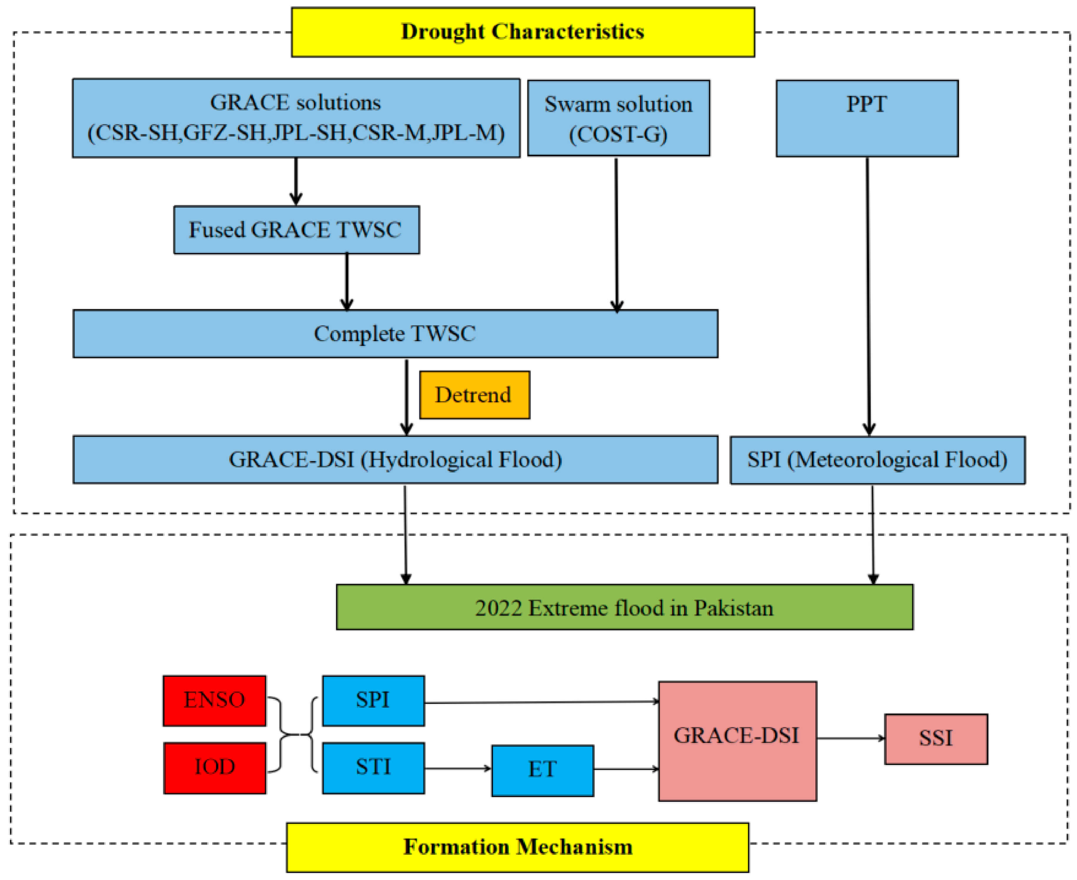
The study roadmap is shown in Figure 2.

5. Results

5.1. TWSC Evaluation

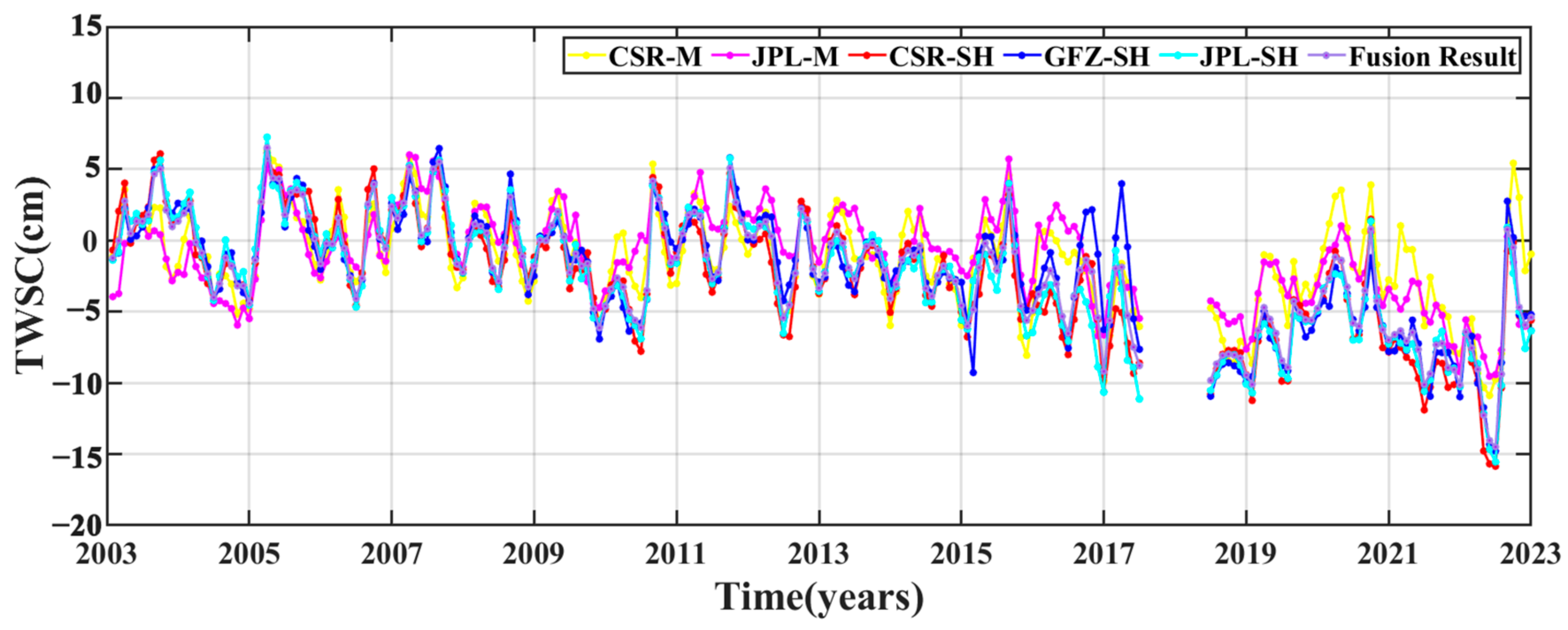
We firstly estimated the uncertainty of four GRACE TWSC results (CSR-SH, 0.96 cm; GFZ-SH, 1.25 cm; JPL-SH, 1.04 cm, CSR-M, 3.66 cm, and GFZ-M, 3.66 cm). It can be seen that there are discrepancies in the uncertainty of five TWSC results. The discrepancy reduces the reliability of the study results based on any single TWSC result. Therefore, we combined the above five TWSC results. Figure 3 demonstrates the five GRACE TWSC results and the fused result in Pakistan between 2003 and 2022. It found that five time series have the same peaks and troughs. The fused result have a strong correlation with four GRACE TWSC results (the correlation coefficients greater than 0.92), and its uncertainty result (0.44 cm) shows that the accuracy of TWSC result has been greatly improved. The above results explains that the fused TWSC result has high reliability and accuracy in Pakistan. Therefore, we used the fused result as the GRACE TWSC in the following study.
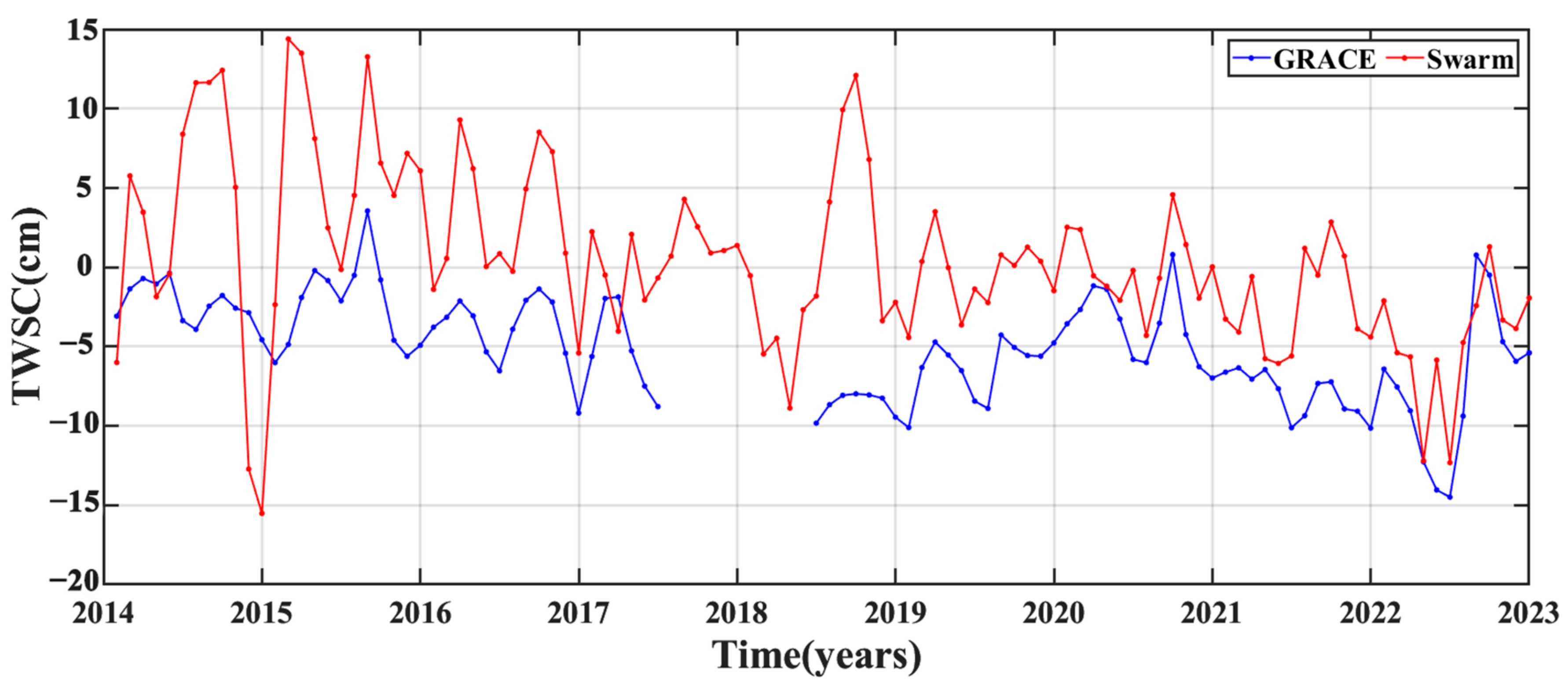
From Figure 3, a data gap (from July 2017 to May 2018) appeared between GRACE and GRACE-FO TWSC results, which brings difficulties to the analysis of hydrological change patterns. Therefore, we used the Swarm TWSC result to fill the gap to construct a continuous complete time series of TWSC observation. To verify the reliability of the Swarm TWSC result, we compared the time series and spatial distribution of uncertainty of GRACE and Swarm TWSC results in Pakistan during the study period (Figure 4 and Table 4). From Figure 4, the GRACE and Swarm TWSC results have the same change trend, and similar peaks and troughs. Their long-term trend changes are very close, but the annual amplitudes and phases have some differences (Table 4). The different annual amplitudes and phases are attributed to the large errors in the Swarm TWSC result [11].
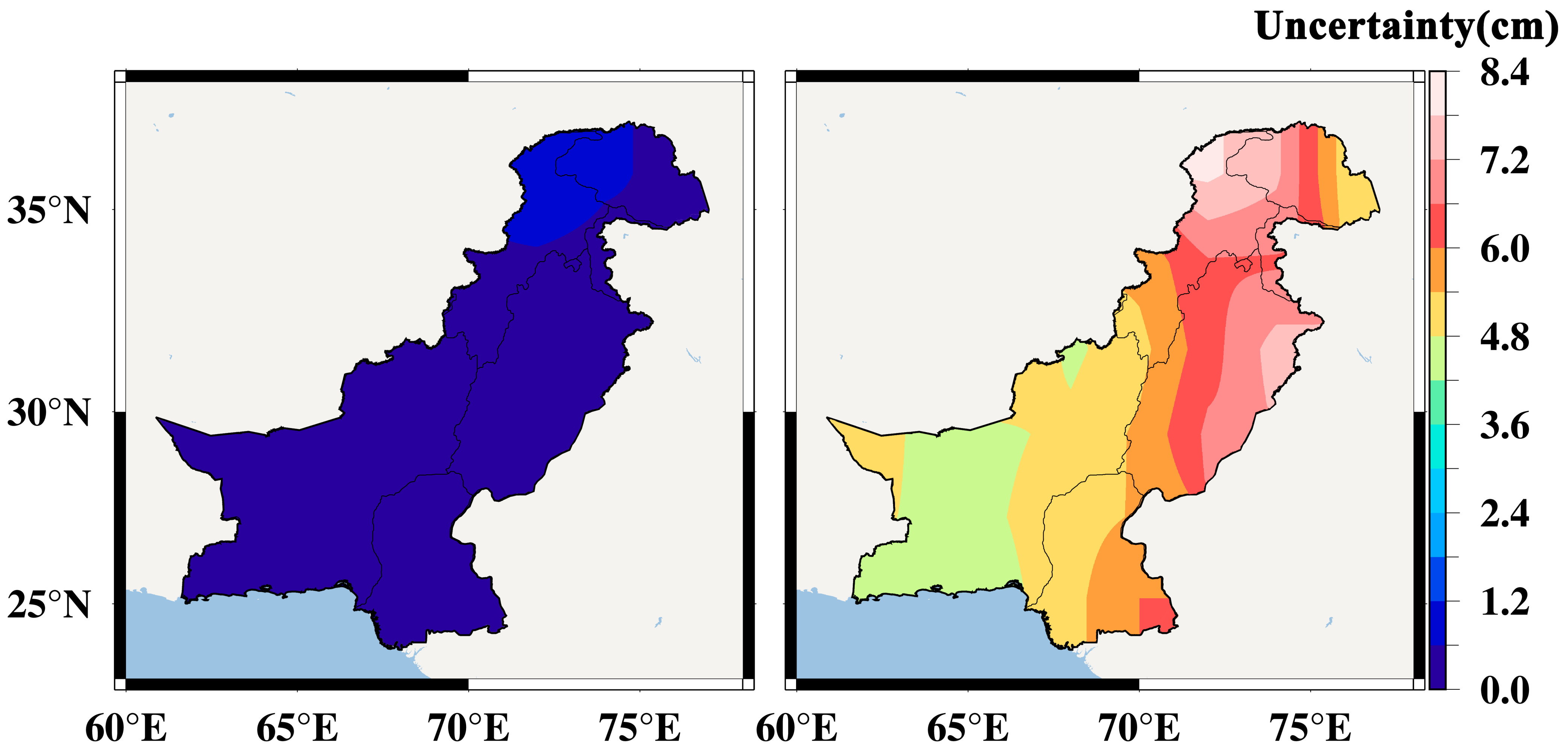
The uncertainties of GRACE TWSC results are significantly smaller than those of Swarm ones (Figure 5). The uncertainties of GRACE TWSC results are all less than 1.2 cm, while those of Swarm ones are from 4.2 cm to 8.4 cm. The maximum of the uncertainties of GRACE TWSC results are concentrated in the parts of KP and GB. The uncertainties of the Swarm TWSC result show a spatial distribution characteristic of being high in the northeast and low in the southwest, and the maximum values are mainly concentrated in the parts of KP and GB, and in the eastern area of Punjab.
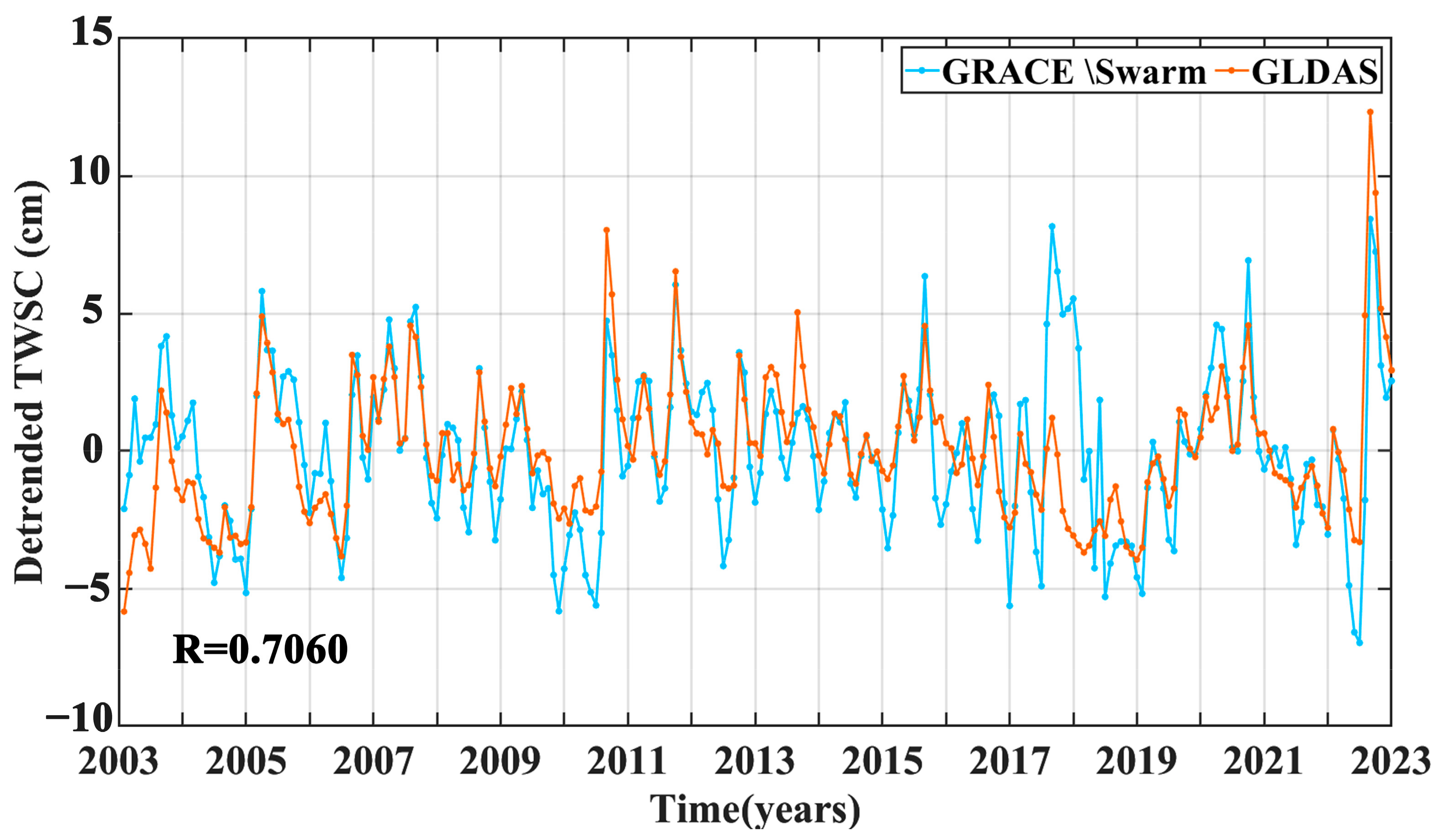
To verify the reliability and applicability of the GRACE/Swarm TWSC results, we compared them with the GLDAS TWSC results. However, groundwater overexploitation exists in Pakistan, and GLDAS TWSC does not reflect human-induced TWSC [32,55]. As the long-term trend mainly reflects the impact of human activities, we detrended the two TWSC results. Figure 6 shows the time series of two detrended TWSC results. It can be seen that the two results have the similar peaks and troughs, and their trends are basically the same. And the two detrended TWSC results have a strong correlation (0.7060). This shows that the GRACE/Swarm TWSC results have a high reliability and applicability in Pakistan.

5.2. Spatiotemporal Evolution of Flood

From Figure 7, we can see that Pakistan is a country which experiences the frequent occurrence of floods and droughts. Positive PPT anomalies appeared between June and August 2022, while TWSC also showed positive anomaly characteristics from August to December 2022 (Figure 7a, red box). The maximum PPT anomaly (3.9 mm) occurred in July, while the TWSC anomaly reached its peak (7.3 cm) in September. Both positive and peak values of PPT anomalies occurred two months earlier than the ones of TWSC. This explains why there is a delay in the TWSC response to PPT (two months). Comparing historical data, the PPT positive anomaly for this flood is the largest between 2003 and 2022, and TWSC positive anomaly is second only to the one between 2017 and 2018. Figure 7b shows the temporal evolution of SPI and GRACE-DSI in Pakistan between 2003 and 2022. In our study, SPI and GRACE-DSI values greater than 0.5 are considered to indicate a flood event. Between June and August 2022, a 3-month flood event occurred (SPIs > 0.5). Because it was caused by excessive PPT, it is called a meteorological flood. And a 5-month flood event occurred from August to December 2022 (GRACE-DSI > 0.5), which was caused by a terrestrial water storage surplus. We call this a hydrological flood. Based on the timeline, it is clear that the hydrological flood is caused by the meteorological flood, and the former lasts longer. Combing the indicators, the PPT-induced extreme meteorological flood is the most severe between 2003 and 2022, and the resulting hydrological flood is second only to the 2017–2018 one.
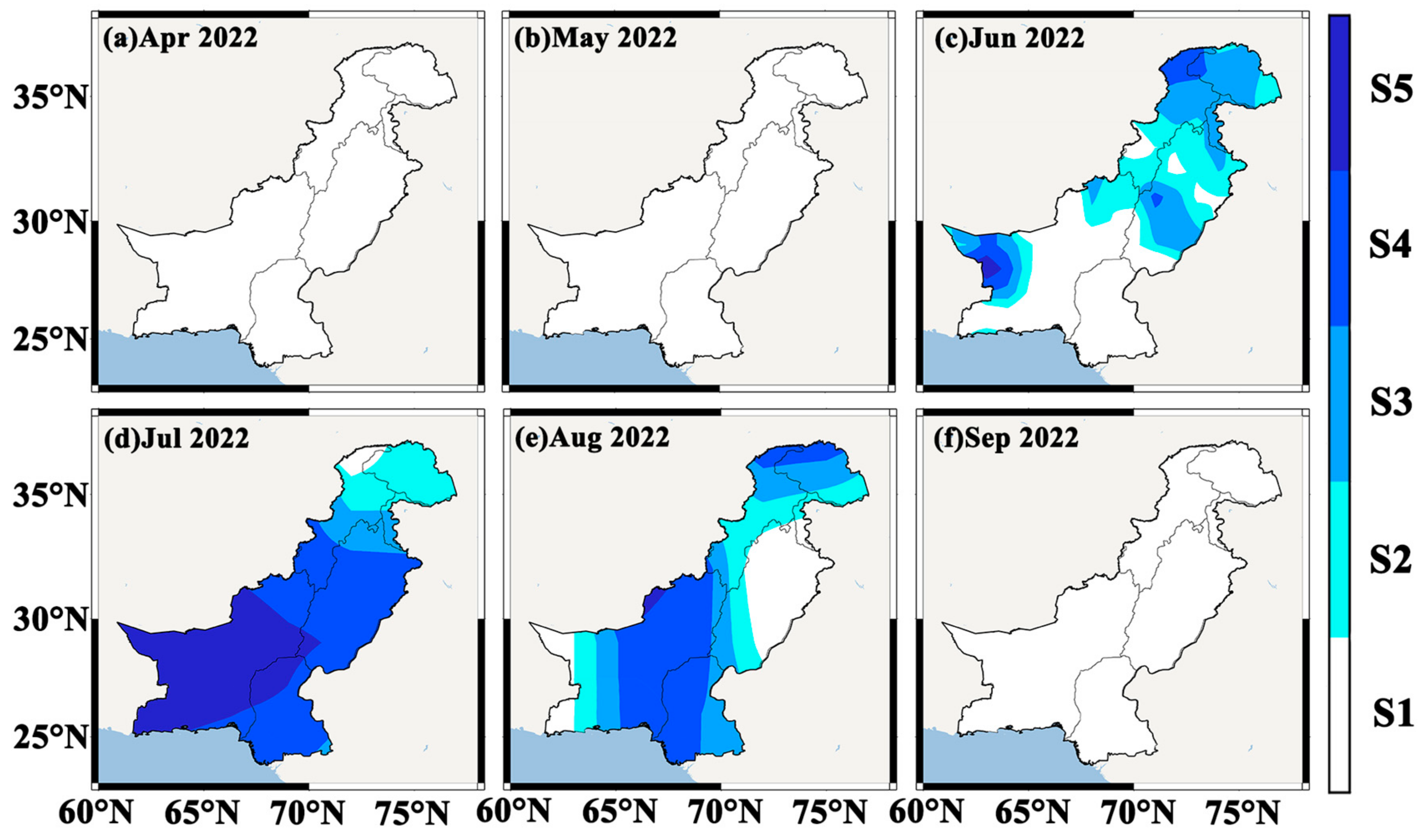
We plotted the spatiotemporal evolution maps of SPI in the flood between April and September 2022 (Figure 8). A meteorological flood (SPI > 0.5) appeared first in June and was concentrated in the northern region, while flooding was also observed in the western part of Balochistan. Flood conditions were mainly light and moderately wet in this month, with some regions experiencing severe wet or even extreme wet conditions. As we enter the month of July, we see that almost the entire territory of Pakistan was wet. Among the various regions, the most severely affected is Balochistan (SPI = 2.354), much of which is under extreme wet conditions. Meteorological flooding is spatially characterized by a south-heavy, north-light distribution. July is also the worst month for meteorological flooding. In August, flood events went into decline. The extreme wet conditions disappeared. Most of Punjab and parts of Balochistan were free from meteorological flooding. By September, the flood event had completely subsided.
We characterized meteorological flooding in different provinces of Pakistan (Table 5). ICT and AK are not included in the statistics due to their small size. Balochistan is the most affected by the flood, whose severity reaches 3.832 and whose peak is the greatest (2.354). GB is the province with the longest duration of the flood (3 months), while all other provinces have only 2 months of flooding. July is the worst time for the flood, with peaks in three provinces occurring in this month. In contrast to the fluctuation of the affected area in other provinces, the affected area in the Sindh has remained basically unchanged at 99.59%. Overall, the two southern provinces (Balochistan and Sindh) and GB were the most severely affected by this meteorological flood.
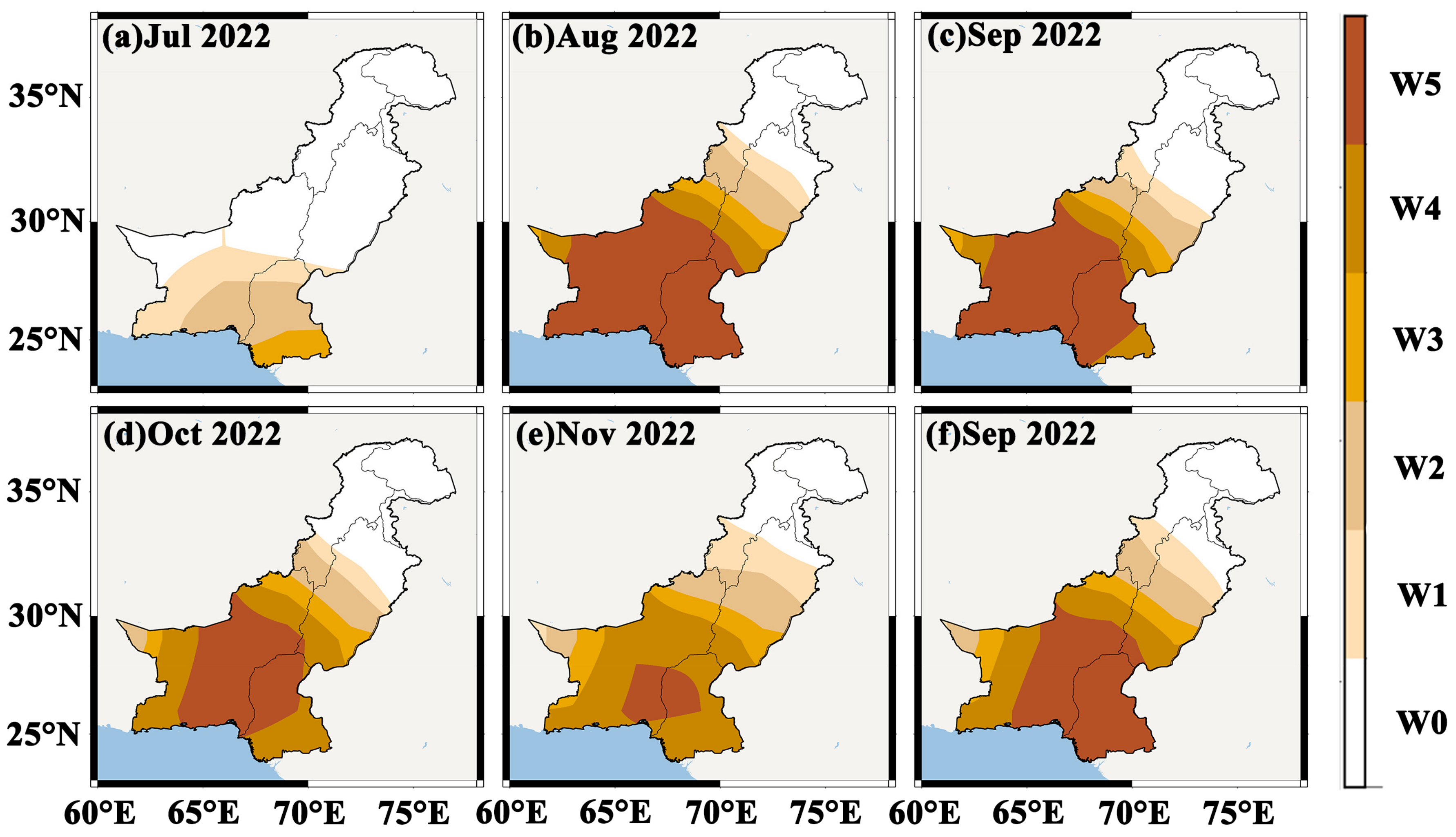
Figure 9 shows the spatiotemporal evolution of a hydrological flood in Pakistan between July and December 2022. In July, the flood was mainly concentrated in the two southern provinces (Balochistan and Sindh). At that time, the flood was dominated by light and moderate wet conditions, with severe wet conditions appeared in the southern of Sindh. Between August and September, the flood continued to push northward and became progressively wetter from north to south. The flood peaked in September, with most areas experiencing exceptional wet conditions. Among all regions, Balochistan and Sindh were almost entirely affected by exceptional wet conditions. From October to December, although the impact of flood continued to grow, it is at the end of its rope. We can clearly see the wetness fading. This indicates that Pakistan weathered this flood event and is beginning to enter a recovery period.
Table 6 illustrates the damage in each province during this hydrological flood event. The worst affected province is Sindh, which was affected by this flood for the longest period (from July to December, six months) and at the highest level of severity (12.139). And all of Sindh was under the shadow of this flood between August and December 2022. Balochistan was the next most affected (severity, 10.187), and it had a relatively short flood duration (five months). Punjab, though also experiencing six months of flood, saw far less severe conditions than the two previously mentioned provinces (4.747). In summary, the flood event was mainly concentrated in the south, especially in Sindh and Balochistan.
To better study the spatial pattern of change in this flood, we mapped the movement trajectory of the flood (Figure 10). From Figure 10a, the trajectory of meteorological flood is characterized by a change from south to north, and the center of gravity of the flood is always located in Balochistan. It is consistent with Balochistan being the province most affected by meteorological flooding. The center of gravity of the hydrological flood pulls repeatedly in a north–south direction at the junction of Sindh and Balochistan (Figure 10b). This fully explains why the worst hit regions of this flood are located in two southern provinces (Sindh and Balochistan).

5.3. Flood Causes

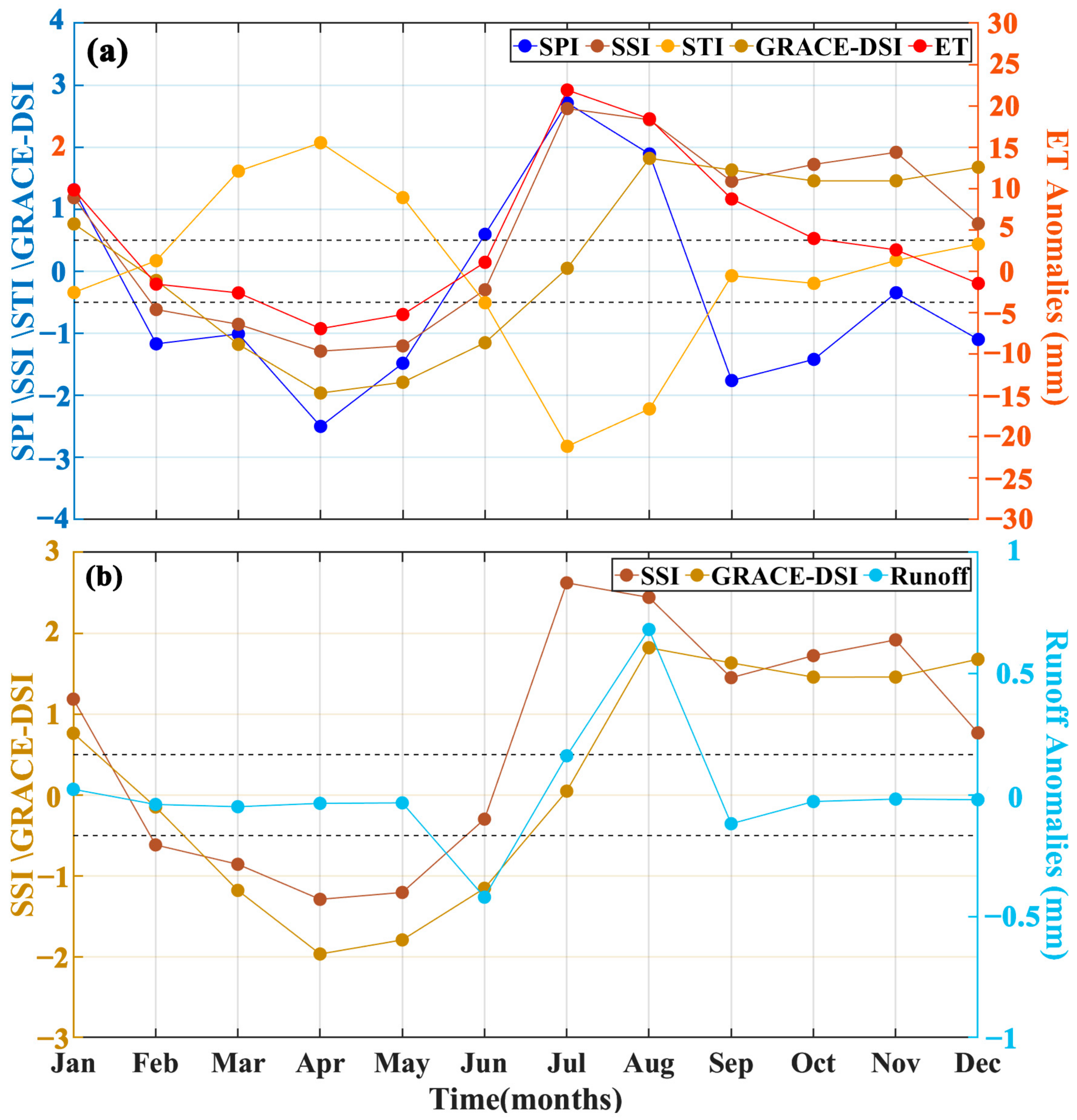
In this section, we analyze the cause of this flood. From Figure 11a, prior to this flood event, Pakistan experienced a drought event from February to June (SPI < −0.5 or GRACE-DSI < −0.5). The drought event was clearly caused by high TEM (STI > 0.5) and low PPT (SPI < −0.5). From March to May, Pakistan experienced 3 months of hot weather. At the same time, PPT was also on the low side (SPI < −0.5) compared to the same period. The scarcity of PPT during this period also caused a shortage of SM (SSI < −0.5, from February to May). During the drought, ET was essentially in a negative anomaly due to the terrestrial water deficit. Although TEM was at a high level (STI > 0.5), there was no water source available for ET.
April was the inflection point for changes in PPT to occur (Figure 11a). In just four months, PPT changed drastically, with the SPI changing from −2.5 (extreme dry) in April to 2.8 (extreme wet) July, an increase of 1.8 per month. Among, the rate was 2.1 per month from May to June and 2.2 per month from June to July. The results suggest that extreme PPT events occurred in Pakistan over a relatively short period of time. And the sharp rise in PPT was accompanied by great fluctuations in SM. SSI increased rapidly from −1.8 to 3.6, an increase of 1.8 per month. Its rate is exactly the same as that of SPI, which means that the increase in SM was caused exclusively by PPT. Therefore, SPI and SSI have the same change trend. The ET anomaly has the opposite trend to STI, but has the same trend as SPI. This shows that ET is completely controlled by PPT. Although STIs were less than −0.5 between June and August, it was still summer, with the highest TEM of the year, and with extreme PPT providing ample water for ET, the ET anomaly rises along with SPI. GRACE-DSI changes along with SSI changes, but the response time for changes was 1–2 months. The inflection points of the SSI trend were in April (from decrease to increase) and July (from increase to decrease), respectively, while those of GRACE-DSI are in May and September, respectively. This is because runoff is at work. The month after SSI peaked, runoff anomalies also peaked (Figure 11b). This suggests that after SM saturation is reached, terrestrial water flows from soil to river and groundwater. In our study, runoff consists of surface runoff and subsurface runoff. Therefore, river and groundwater have a regulating effect on SM. The response time of this regulating effect is one month. After runoff reached its peak, GRACE-DSI also reached its peak in the following month.
In summary, the heavy PPT over a short period of time transformed Pakistan region from extremely dry to extreme wet, and the terrestrial ecosystems had no time to adapt to such a drastic hydrological change. This is an important reason for this flood.
La Niña events have occurred in Northern Hemisphere winter for three consecutive years from September 2020 to December 2022 (Figure 12a). Meteorologists refer to this phenomenon as a triple La Niña event [56]. The last time the phenomenon occurred was in 1998–2001. The impact of La Niña event on East Asia is mainly through the control of the location and intensity of the west Pacific subtropical high (WPSH) [57]. In La Niña years, WPSH is strengthened and its position is more north and west than normal. A strong WPSH blocks the transport of water vapor from the low-latitude oceans to South China [58]. From Figure 12b, we see that the triple La Niña event coincided with three consecutive years of negative IOD events (DMI is negative) in the Indian Ocean. When the negative IOD event occurred, there is a higher sea surface temperature on the eastern side of the Indian Ocean than on the western side, which results in a west-to-east movement of convective activity over the Indian Ocean. It brings a large amount of water vapor to the eastern Indian Ocean [59,60]. Therefore, atmospheric circulation anomalies are a prerequisite for the 2022 heavy PPT in Pakistan.
To articulate how the two extreme climate events caused heavy PPT in Pakistan, we plotted the map of standardized anomaly of geopotential height at 500 hPa around Eurasia from May to August 2022 (Figure 13). In climatology, the 500 hPa level is the layer where atmospheric circulation and fronts are most active. Therefore, it usually utilized to analyze the mid-tropospheric flows. In May, a strong negative anomaly appeared in the Ural Mountains, and its southern extension reached the Caspian Sea, with the trough deeper than usual. Two positive anomalies were generated in the northwest (Altai) and southeast (Red Sea) directions of Pakistan. In particular, the ridge height of the positive anomaly located in the Altai was significantly higher than in previous years. Pakistan was right in the middle of two high pressures and its air pressure is higher than normal (Figure 13a). Therefore, Pakistan was in a state of high TEM and little PPT at the time (Figure 11a,b). The 5880 gpm characteristic line (the purple contour line) was located in roughly the same place as the climatological state (the green contour line). By June, the negative anomaly in the Ural Mountains moved to Western Siberia, but its strength has weakened considerably. The strong positive anomaly in the Altai weakened and shifted to Northwest China, with its southern edge reaching northeast India and the Bay of Bengal. It blocked the traditional eastward route of water vapor from the East Indian Ocean, and the eater vapor transport was redirected to North India and Pakistan [61]. The positive anomaly in the Red Sea shifted eastward into the Persian Gulf and covered the Iranian Plateau, blocking the continued westward movement of water vapor from the eastern Indian Ocean. At this time, Pakistan was under the negative anomaly. Such meteorological conditions favor heavy PPT in Pakistan [62]. The 5880 gpm characteristic line moved significantly north, largely overlapping with the position of the climatological state.
In July, a strong positive anomaly has formed over the Tibetan Plateau, which covered from the Iranian Plateau to the upper reaches of Yangtze River, and its southeastern edge even reached the Strait of Malacca. Meanwhile, WPSH extended westward to the southeast coast of China. Subtropical high pressure from the west has extended to the Tibetan Plateau. It virtually blocked the north-east transmission of water vapor from the East Indian Ocean. The negative anomaly in the middle of Pakistan moved to the southern, which has allowed the heavy PPT to continue. In August, the positive anomaly across northern Pakistan began to recede, shifting from the Tibetan Plateau to the Yangtze River basin. Subtropical high pressure from the west retreated to the Iranian Plateau. At the time, a significant trough of low pressure formed northwest of Pakistan, allowing a northward passage of Indian Ocean moisture. The water vapor that had gathered over Pakistan was relieved, and the heavy PPT entered its end phase.

6. Discussion

6.1. Flood Propagation

Flooding does not happen overnight. There is a process of propagation and evolution of the water surplus state from conception, onset, and catastrophe. We have therefore divided the flood event into three parts, namely meteorological flood, agricultural flood, and hydrological flood. From Figure 9c, the meteorological flood (SPI ≥ 0.5) lasted only three months (June to August), peaking in July (SPI = 2.8, S4). Mallapaty [62] indicates that Pakistan has been hit by several heavy PPT since June 2022. The agricultural flood (SSI ≥ 0.5) occurred 1 month later than the meteorological flood (July to December), but it peaks (SSI = 3.6) in the first month and then declined slowly. In Figure 9d, the hydrological flood (GRACE-DSI ≥ 0.5) began in August and continued through December, two months and one month after the meteorological and agricultural floods, respectively, and peaks (GRACE-DSI = 1.8, W4) in September. The results outline the propagation process of the flood in meteorological, agricultural, and terrestrial ecosystems. The flood first occurred in meteorological system and then spread to agricultural and terrestrial ecosystems, but the flood lasted much longer in the agricultural (six months) and terrestrial ecosystems (five months) than in the meteorological system (three months). The agricultural system is much more affected than terrestrial ecosystem, and the impact of the flood on the agriculture and terrestrial ecosystems in Pakistan is far-reaching.

6.2. Flood Impact

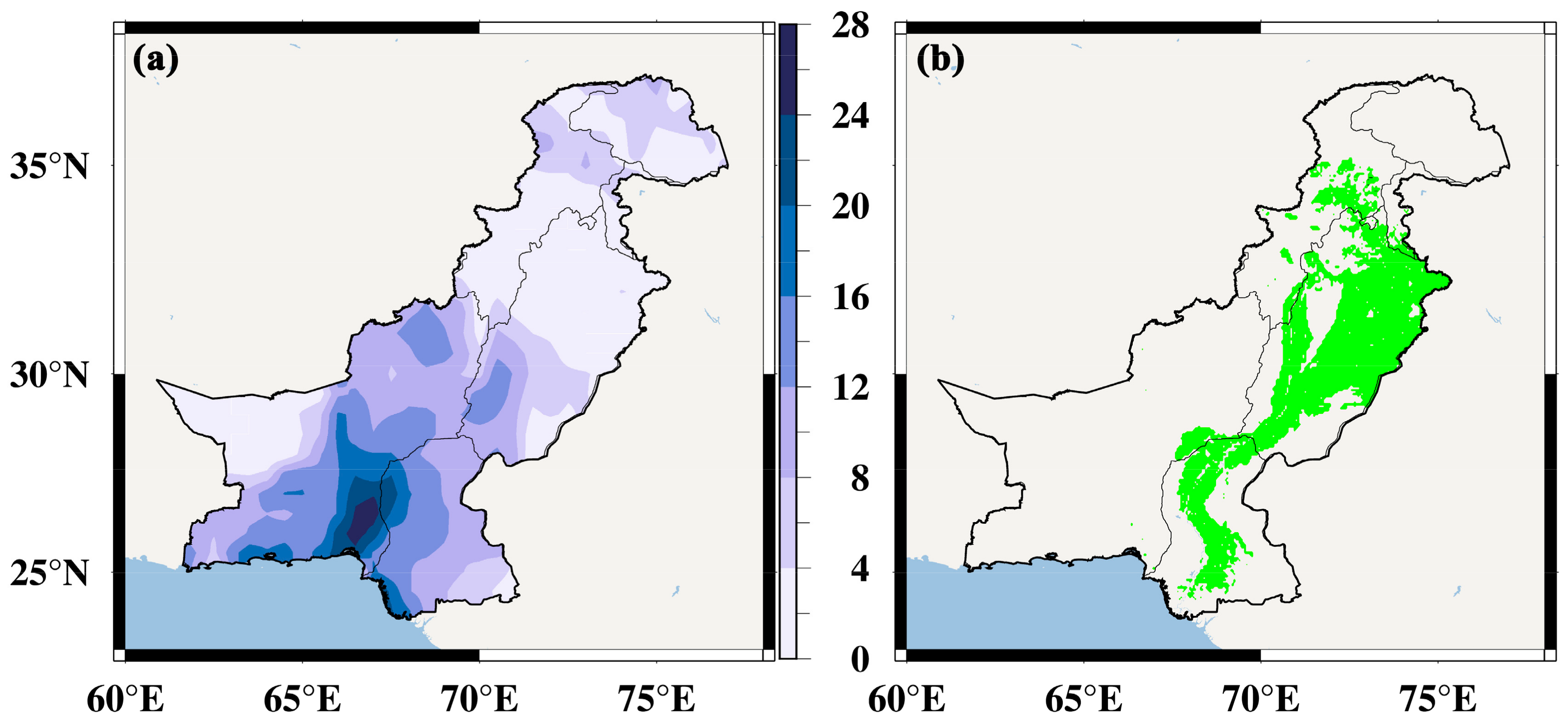
Since Pakistan’s national economy is mainly based on agriculture, we focus on the impact of the flood on local agriculture. In our study, SSI was used to evaluate the severity of agricultural flood (Figure 14a). The southern coast and the border between Balochistan and Sindh are the worst affected regions of the flood. Figure 14b shows the spatial distribution of cropland in Pakistan. From this figure, Pakistan’s croplands are concentrated in Sindh and Punjab, and partly in KP. Comparing Figure 14a,b, all the croplands are affected to varying degrees by this flood. The croplands located in the southern of Punjab and Sindh are the most severely affected by the flood, which accounts for approximately 50% of the total croplands. Local news demonstrates that there are about four million hectares of agricultural land affected by the flood [63]. It would greatly increase the likelihood of famine in the aftermath of the flood. Pakistan has sent a request to the World Food Programme for emergency assistance [64]. The United Nations has launched a USD 161 million emergency fund-raising appeal for Pakistan. The funds provide critical food and cash assistance to nearly 1 million people in Balochistna, Sindh, Punjab, and KP [65].

6.3. Driving Factors of the Flood

The findings suggest a very strong connection between global extreme climate events and the flood. Negative IOD events alter the atmospheric circulation over the Indian Ocean, transporting a steady stream of water vapor from the western side of the Indian Ocean over the eastern Indian Ocean. These water vapors continue to be transported northward through the Indian Ocean summer monsoon, and were originally supposed to continue onward to northwest and northeast, respectively, after encountering the Himalayas on the Indian Subcontinent. However, a strong WPSH entrenched in South China and the Central-South Peninsula under the influence of La Niña event, blocking the delivery of water vapor in the northeastern direction. As a result, a large amount of water vapor was transported over Pakistan. At this time, the vast region from the Iranian Plateau all the way to the Tibetan Plateau was also controlled by high pressure, preventing water vapor from continuing northward and westward. Therefore, water vapor was massing over Pakistan. Nanditha et al. [66] observed that the presence of up to 80 mm of total column water vapor accumulation over Pakistan in August 2022. Thus, the heavy PPT caused by extreme climate events was the main factor that led to the 2022 Pakistan flood.
In addition, the contribution of the persistent hot weather from March to May (Figure 9a) should not be overlooked. Pakistan has a large number of alpine glaciers in its northern mountains [67]. These glaciers are melting rapidly as temperatures rise sharply, causing a rapid increase in runoff in the upper reaches of Indus River basin [62]. And human-induced global warming is also a major cause of the frequency of extreme PPT events [68,69].

7. Conclusions

In this study, we integrated multiple satellite gravity data, meteorological data, hydrological data, and satellite remote sensing data to review the 2022 summer severe flood in Pakistan to trace its cause and assess the disaster damage. The study results are summarized in the following three points.
Firstly, our TWSC results, based on five GRACE/GRACE-FO solutions by using the GTCH and least square methods, are substantially more accurate than any single GRACE/GRACE-FO solution. By utilizing a Swarm TWSC result to fill the data gap between GRACE and GRACE-FO missions, we obtained a highly reliable and applicable time series of Pakistan’s TWSC over 20 consecutive years.
Secondly, by analyzing the 20-year TWSC time series, we found that Pakistan is a flood- and drought-prone country. The 2022 severe flood lasted only three months, but its impact on the local agricultural system and terrestrial ecosystem amounted for six and five months, respectively. Balochistan and Sindh are the two provinces most affected by this severe flood.
Finally, the severe flood was created under the influence of global extreme climate events (La Niña and negative IOD events). The extreme climate events altered the atmospheric circulation patterns over Eurasia, causing large amounts of Indian Ocean water vapor to converge over Pakistan, which in turn led to heavy PPT. This was the main driver of the flood event. Glacial melting caused by high temperature contributed to the flood.
Our result has a certain reference value for understanding the physical mechanisms of the impact of extreme climate events on regional climate change, and provide strong data support for the development of scientific and reasonable local policies for the defense of flood and drought disasters.

Author Contributions

Conceptualization, L.C. and J.A.; methodology, L.C. and Y.M.; software, J.M. and Y.L.; resources, J.A.; data curation, J.M. and G.W.; writing—original draft preparation, L.C.; writing—review and editing, L.C. and Z.Z.; project administration, L.Z.; funding acquisition, L.C. All authors have read and agreed to the published version of the manuscript.

Funding

This research was funded by the National Natural Science Foundation of China (41931074, 42074172, 42171141); 2023 China Student Innovation Training Programme Project (202311079005, 202311079007, 202311079008); Max-Planck-Society and the Chinese Academy of Sciences within the LEGACY (“Low-Frequency Gravitational Wave Astronomy in Space”) collaboration (M.IF.A.QOP18098).

Data Availability Statement

Data are contained within the article.

Acknowledgments

We are grateful to CSR, GFZ, and JPL for providing GRACE solution; the COST-G for providing Swarm solution; the European Center for Medium-Range Weather Forecasts for providing PPT, SM, TEM, and runoff data; the Global Land Evaporation Amsterdam Model for providing ET data; the Goddard Space Flight Center for providing GLDAS-2.1 data; and the National Oceanic and Atmospheric Administration for providing climate index and geopotential height data.

Conflicts of Interest

The authors declare no conflicts of interest.

References

  1. Merz, B.; Kreibich, H.; Schwarze, R.; Thieken, A. Review article “Assessment of economic flood damage”. Nat. Hazard Earth Syst. Sci. 2010, 10, 1697–1724. [Google Scholar] [CrossRef]
  2. Cui, L.; He, M.; Zou, Z.; Yao, C.; Wang, S.; An, C.; Wang, X. The Influence of Climate Change on Droughts and Floods in the Yangtze River Basin from 2003 to 2020. Sensors 2022, 22, 8178. [Google Scholar] [CrossRef] [PubMed]
  3. Hallegatte, S.; Green, C.; Nicholls, R.; Corfee-Morlot, J. Future flood losses in major coastal cities. Nat. Clim. Change 2013, 3, 802–806. [Google Scholar] [CrossRef]
  4. Hall, J.; Arheimer, B.; Borga, M.; Brázdil, R.; Claps, P.; Kiss, A.; Kjeldsen, T.; Kriaučiūnienë Kundzewicz, Z.; Lang, M.; Llasat, M.; et al. Understangding flood regime changes in Europe: A state-of -the-art assessment. Hydrol. Earth Syst. Sci. 2014, 18, 2735–2772. [Google Scholar] [CrossRef]
  5. The West Is Ignoring Pakistan’s Super-Floods. Heed This Warning: Tomorrow It Will Be You. Available online: https://www.theguardian.com/commentisfree/2022/sep/08/pakistan-floods-climate-crisis (accessed on 19 October 2023).
  6. Rich Countries Caused Pakistan’s Catastrophic Flooding. Their Response? Inertia and Apathy. Available online: https://www.theguardian.com/commentisfree/2022/sep/05/rich-countries-pakistan-flooding-climate-crisis-cop27 (accessed on 19 October 2023).
  7. Lotto, F.; Zachariah, M.; Saeed, F.; Siddiqi, A.; Shahzad, K.; Mushtaq, H.; Arulalan, T.; AchutaRao, K.; Chaithra, S.; Barnes, C.; et al. Climate change likely increased extreme monsoon rainfall, flooding highly vulnerablecommunities in Pakistan. Environ. Res. Climate 2023, 2, 025001. [Google Scholar]
  8. Sarkar, S. Pakistan floods pose serious health challenges. BMJ 2022, 378, 2141. [Google Scholar] [CrossRef]
  9. Mirza, M. Climate change, flooding in South Asia and implications. Regional Environ. Change 2011, 11, 95–107. [Google Scholar] [CrossRef]
  10. Owusu, M.; Nursey-Bray, M.; Rudd, D. Gendered perception and vulnerability to climate change in urban slum communities in Accra, Ghana. Regional Environ. Change 2019, 19, 13–25. [Google Scholar] [CrossRef]
  11. Hirabayashi, Y.; Mahendran, R.; Koirala, S.; Konoshima, L.; Yamazaki, D.; Watanabe, S.; Kim, H.; Kanae, S. Global flood risk under climate change. Nat. Clim. Change 2013, 3, 816–821. [Google Scholar] [CrossRef]
  12. Alfieri, L.; Bisselink, B.; Dottori, F.; Naumann, G.; De Roo, A.; Salamon, P.; Wyser, K.; Feyen, L. Global projections of river flood risk in a warmer world. Earth’s Future 2017, 5, 171–182. [Google Scholar] [CrossRef]
  13. Global Climate Risk Index. Available online: https://www.germanwatch.org/sites/default/files/Global%20Climate%20Risk%20Index%202021_2.pdf (accessed on 19 October 2023).
  14. Li, X.; Zhong, B.; Li, J.; Wang, H. Investigating terrestrial water storage changes and their driving factors in the Southwest River basin of China using geodetic data. IEEE Trans. Geosci. Remote sens. 2023, 61, 5922115. [Google Scholar] [CrossRef]
  15. Cui, L.; Luo, C.; Yao, C.; Zou, Z.; Wu, G.; Li, Q.; Wang, X. The influence of climate change on forest fires in Yunnan province, Southwest China detected by GRACE satellites. Remote Sens. 2022, 14, 712. [Google Scholar] [CrossRef]
  16. Zhou, H.; Luo, Z.; Zhou, Z.; Li, Q.; Zhong, B.; Lu, B.; Hsu, H. Impact of different kinematic empirical parameters processing strategies on temporal gravity field model determination. J. Geophys. Res. Solid Earth 2018, 123, 252–276. [Google Scholar] [CrossRef]
  17. Zhong, B.; Li, Q.; Li, X.; Chen, J. Basin-scale terrestrial water storage changes inferred from GRACE-based geopotential differences: A case study of the Yangtze River basin, China. Geophys. J. Int. 2023, 223, 1318–1338. [Google Scholar] [CrossRef]
  18. Wahr, J.; Molenaar, M.; Bryan, F. Time variability of the Earth’s gravity field: Hydrological and oceanic effects and their possible detection using GRACE. J. Geophys. Res. Solid Earth 1998, 103, 30205–30229. [Google Scholar] [CrossRef]
  19. Zou, Z.; Li, Y.; Cui, L.; Yao, C.; Xu, C.; Yin, M.; Zhu, C. Spatiotemporal evaluation of the flood potential index and its driving factors across the Volga River basin based on combined satellite gravity observation. Remote Sens. 2023, 15, 4144. [Google Scholar] [CrossRef]
  20. Reager, J.; Famiglietti, J. Global terrestrial water storage capacity and flood potential using GRACE. Geophys. Res. Lett. 2009, 36, L23402. [Google Scholar] [CrossRef]
  21. Chen, J.; Wilson, C.; Tapley, B. The 2009 exceptional Amazon flood and interannual terrestrial water storage change observed by GRACE. Water Resour. Res. 2010, 46, WE009383. [Google Scholar] [CrossRef]
  22. Long, D.; Shen, Y.; Sun, A.; Hong, Y.; Longuevergne, L.; Yang, Y.; Li, B.; Chen, L. Drought and flood monitoring for a large karst plateau in Southwest China using extended GRACE data. Remote Sens. Environ. 2014, 155, 145–160. [Google Scholar] [CrossRef]
  23. Molodtsova, T.; Molodtsov, S.; Kirilenko, A.; Zhang, X.; Vanlooy, J. Evaluating flood potential with GRACE in the United States. Nat. Hazards Earth Syst. Sci. 2016, 16, 1011–1018. [Google Scholar] [CrossRef]
  24. Yirdaw, S.Z.; Snelgrove, K.R.; Agboma, C.O. GRACE satellite observations of terrestrial moisture changes for drought characterization in the Canadian Prairie. J. Hydrolo. 2008, 356, 84–92. [Google Scholar] [CrossRef]
  25. Wang, J.H.; Jiang, D.; Huang, Y.H.; Wang, H. Drought analysis of the Haihe River basin based on GRACE terrestrial water storage. Sci. World J. 2014, 2014, 578372. [Google Scholar] [CrossRef] [PubMed]
  26. Yi, H.; Wen, L. Satellite gravity measurement monitoring terrestrial water storage and drought in the continental United States. Sci. Rep. 2016, 6, 19909. [Google Scholar] [CrossRef] [PubMed]
  27. Cui, L.; Yin, M.; Huang, Z.; Yao, C.; Wang, X.; Lin, X. The drought events over the Amazon River basin from 2003 to 2020 detected by GRACE/GRACE-FO and Swarm satellites. Remote Sens. 2022, 14, 2887. [Google Scholar] [CrossRef]
  28. Xiong, J.; Yin, J.; Guo, S.; Gu, L.; Xiong, F.; Li, N. Integrated flood potential index for flood monitoring in the GRACE era. J. Hydrol. 2021, 603, 127115. [Google Scholar] [CrossRef]
  29. Da Encarnação, T.; Visser, P.; Arnold, D.; Bezdek, A.; Doornbos, E.; Ellmer, M.; Guo, J.; van den IJssel, J.; Iorfida, E.; Jäggi, A.; et al. Description of the multi-approach gravity field models from Swarm GPS data. Earth Syst. Sci. Data 2020, 12, 1385–1417. [Google Scholar] [CrossRef]
  30. Cui, L.; Song, Z.; Luo, Z.; Zhong, B.; Wang, X.; Zou, Z. Comparison of terrestrial water storage changes derived from GRACE/GRACE-FO and Swarm: A case study in the Amazon River Basin. Water 2020, 12, 3128. [Google Scholar] [CrossRef]
  31. Zhang, C.; Shum, C.; Bezdek, A.; Bevis, M.; de Encarnação, T.; Tapley, B.; Zhang, Y.; Su, X.; Shen, Q. Rapid mass loss in west Antractica revealed by Swarm Gravimetry in the Absence of GRACE. Geophys. Res. Lett. 2021, 48, e2021GL095141. [Google Scholar] [CrossRef]
  32. Cui, L.; Yin, M.; Zou, Z.; Yao, C.; Xu, C.; Li, Y.; Mao, Y. Spatiotemporal change in evapotranspiration acorss the Indus River basin detected by combining GRACE/GRACE-FO and Swarm observations. Remote Sens. 2023, 15, 4469. [Google Scholar] [CrossRef]
  33. Abid, M.; Scheffran, J.; Schneider, U.; Elahi, E. Farmer perceptions of climate change, observed trend and adaptation of agriculture of Pakistan. Environ. Manag. 2019, 63, 110–123. [Google Scholar] [CrossRef]
  34. Abid, M.; Schilling, J.; Scheffran, J.; Zulfiqar, F. Climate change vulnerability, adaption and risk perceptions at farm level in Punjab, Pakistan. Sci. Total Environ. 2016, 547, 447–460. [Google Scholar] [CrossRef] [PubMed]
  35. Cui, L.; Zhang, C.; Yao, C.; Luo, Z.; Wang, X.; Li, Q. Analysis of the influencing factors of drought events based on GRACE data under different climatic conditions: A case study in Mainland China. Water 2021, 13, 2575. [Google Scholar] [CrossRef]
  36. Jean, Y.; Meyer, U.; Jäggi, A. Combination of GRACE monthly gravity field solutions from different processing strategies. J. Geod. 2018, 92, 1313–1328. [Google Scholar] [CrossRef]
  37. Hersbach, H.; Bell, B.; Berrisford, P.; Hirahara, S.; Horányi, A.; Muñoz-Sabater, J.; Nicolas, J.; Peubey, C.; Radu, R.; Schepers, D.; et al. The ERA5 global reanalysis. Q. J. Royal Meteorol. Soc. 2020, 146, 1999–2049. [Google Scholar] [CrossRef]
  38. Khan, M.; Liaqat, U.; Baik, J. Stand-alone uncertainty characterization of GLEAM, GLDAS and MOD16 evapotranspiration products using an extended triple collocation approach. Agric. Forest Meteorol. 2018, 252, 256–268. [Google Scholar] [CrossRef]
  39. Martens, B.; Gonzalez Miralles, D.; Lievens, H.; Van Der Schalie, R.; De Jeu, R.; Fernández-Prieto, D.; Beck, H.; Dorigo, W.; Verhoest, N. GLEAM v3: Satellite-based land evaporation and root-zone soil moisture. Geosci. Model Dev. 2017, 10, 1903–1925. [Google Scholar] [CrossRef]
  40. Cayan, D.; Redmond, K.; Riddle, L. ENSO and hydrologic extremes in the western United States. J. Clim. 2010, 12, 2881–2893. [Google Scholar] [CrossRef]
  41. Cui, L.; Chen, X.; An, J.; Yao, C.; Su, Y.; Zhu, C.; Li, Y. Spatiotemporal variation characteristics of drought and their connection to climate variability and human activity in the Pearl River basin, South China. Water 2023, 15, 1720. [Google Scholar] [CrossRef]
  42. Zhou, Z.; Xie, S.; Zhang, R. Historic Yangtze flooding of 2020 tied to extreme Indian Ocean conditions. Proc. Natl. Acad. Sci. USA 2021, 118, e2022255118. [Google Scholar] [CrossRef]
  43. Rodell, M.; Houser, P.; Jambor, U.; Gottschalck, J.; Mitchell, K.; Meng, C.; Arsenault, K.; Cosgrove, B.; Radakovich, J.; Bosilovich, M.; et al. The Global Land Data Assimilation System. Bull. American Meteorol. Soc. 2004, 85, 381–394. [Google Scholar] [CrossRef]
  44. MODIS Land Cover Type/Dynamics. Available online: https://modis.gsfc.nasa.gov/data/dataprod/mod12.php (accessed on 19 October 2023).
  45. Zhang, B.; Liu, L.; Yao, Y.; van Dam, T.; Khan, S.A. Improving the estimate of the secular variation of Greenland ice mass in the recent decades by incorporating a stochastic process. Earth Planet Sci. Lett. 2020, 549, 116518. [Google Scholar] [CrossRef]
  46. Long, D.; Pan, Y.; Zhou, J.; Chen, Y.; Hou, X.; Hong, Y.; Scanlon, B.; Longuevergne, L. Global analysis of spatiotemporal variability in merged total water storage changes using multiple GRACE products and global hydrological models. Remote Sens. Environ. 2017, 192, 198–216. [Google Scholar] [CrossRef]
  47. Cui, L.; Zhu, C.; Wu, Y.; Yao, C.; Wang, X.; An, J.; Wei, P. Natural- and human-induced influences on terrestrial water storage change in Sichuan, Southwest China from 2003 to 2020. Remote Sens. 2022, 14, 1369. [Google Scholar] [CrossRef]
  48. Bai, H.; Ming, Z.; Zhong, Y.; Zhong, M.; Kong, D.; Ji, B. Evaluation of evapotranspiration for exorheic basins in China using an improved estimate of terrestrial water storage change. J. Hydrol. 2022, 610, 127885. [Google Scholar] [CrossRef]
  49. Cui, L.; Zhu, C.; Zou, Z.; Yao, C.; Zhang, C.; Li, Y. The spatiotemporal characteristics of wildfires across Australia and their connection to extreme climate based on a combined hydrological drought index. Fire 2023, 6, 42. [Google Scholar] [CrossRef]
  50. Vicente-Serrano, S. Differences in spatial patterns of drought on different time scales: An analysis of the Iberian Peninsula. Water Resour. Manag. 2006, 20, 37–60. [Google Scholar] [CrossRef]
  51. Cui, L.; Zhang, C.; Luo, Z.; Wang, X.; Li, Q.; Liu, L. Using the local drought data and GRACE/GRACE-FO data to charactrize the drought events in Mainland China from 2002 to 2020. Appl. Sci. 2021, 11, 9594. [Google Scholar] [CrossRef]
  52. Hao, Z.; Aghakouchak, A. Multivariate standardizad drought Index: A parametric multi-index model. Adv. Water Resour. 2013, 57, 12–18. [Google Scholar] [CrossRef]
  53. Li, J.; Chunyu, X.; Huang, F. Land Use Pattern Changes and the Driving Forces in the Shiyang River Basin from 2000 to 2018. Sustainability 2022, 15, 154. [Google Scholar] [CrossRef]
  54. Cui, L.; Zhong, L.; Meng, J.; An, J.; Zhang, C.; Li, Y. Spatiotemporal evolution features of the 2022 compound hot and drought event over the Yangtze River basin. Remote Sens. 2024, 16, 1367. [Google Scholar] [CrossRef]
  55. Qureshi, A.; Mc Cornick, P.; Sarwar, A.; Sharma, B. Chanllenges and prospects of sustainable groundwater management in the Indus basin, Pakistan. Water Resour. Mag. 2010, 24, 1551–1569. [Google Scholar] [CrossRef]
  56. “Triple” La Niña Event. Available online: https://baijiahao.baidu.com/s?id=1748984438589596831&wfr=spider&for=pc (accessed on 19 October 2023).
  57. La Niña Times Three. Available online: https://earthobservatory.nasa.gov/images/150691/la-nina-times-three (accessed on 19 October 2023).
  58. Subtropical High Pressure, Why This Summer Is Abnormal. Available online: http://finance.people.com.cn/n1/2022/0905/c1004-32519166.html (accessed on 19 October 2023).
  59. Webster, P.; Moore, A.; Loschnigg, J.; Leben, R. Coupled ocean-atmospjere dynamics in the Indian Ocean during 1997–1998. Nature 1999, 401, 356–360. [Google Scholar] [CrossRef] [PubMed]
  60. Indian Ocean Dipole. Available online: https://www.jamstec.go.jp/aplinfo/sintexf/e/iod/about_iod.html (accessed on 19 October 2023).
  61. Climate Change Could Increase Heavy Rainfall in Pakistan. Available online: https://new.qq.com/rain/a/20220920A06N6E00 (accessed on 19 October 2023).
  62. Why Are Pakistan’s Floods so Extreme This Year? Available online: https://www.nature.com/articles/d41586-022-02813-6 (accessed on 19 October 2023).
  63. Mapping the Scale of Damage by the Catastrophic Pakistan Floods Infographic News Al Jazeera. Available online: https://www.aljazeera.com/news/longform/2022/9/16/mapping-the-scale-of-destruction-of-the-pakistan-floods (accessed on 19 October 2023).
  64. Floods Ravage Pakistan, WFP Scales up Assistance. Available online: https://www.deepl.com/translator#zh/en (accessed on 19 October 2023).
  65. United Nations and Pakistan Launch Emergency Fund-Raising Progamme for Floods. Available online: https://www.gdtv.cn/tv/32764f13b4f5b9e40f08889189faee43 (accessed on 19 October 2023).
  66. Nanditha, J.; Kushwaha, A.; Singh, R.; Malik, I.; Solanki, H.; Chuphal, D.; Danger, S.; Mahto, S.; Vegad, U.; Mishra, V. The Pakistan flood of August 2022: Causes and implications. Earth’s Future 2023, 11, e2022EF003230. [Google Scholar] [CrossRef]
  67. Climate Change Made Devastating Early Heat in India and Pakistan 30 Times More Likely. Available online: https://rcc.imdpune.gov.in/Annual_Climate_Summary/annual_summary_2015.pdf (accessed on 19 October 2023).
  68. O’Gorman, P. Precipitation extremes under climate change. Current Clim. Change Rep. 2015, 1, 49–59. [Google Scholar] [CrossRef] [PubMed]
  69. Pfahl, S.; O’Gorman, P.; Fischer, E. Understanding the regional pattern of projected future changes in extreme precipitation. Nat. Clim. Change 2017, 7, 423–427. [Google Scholar] [CrossRef]
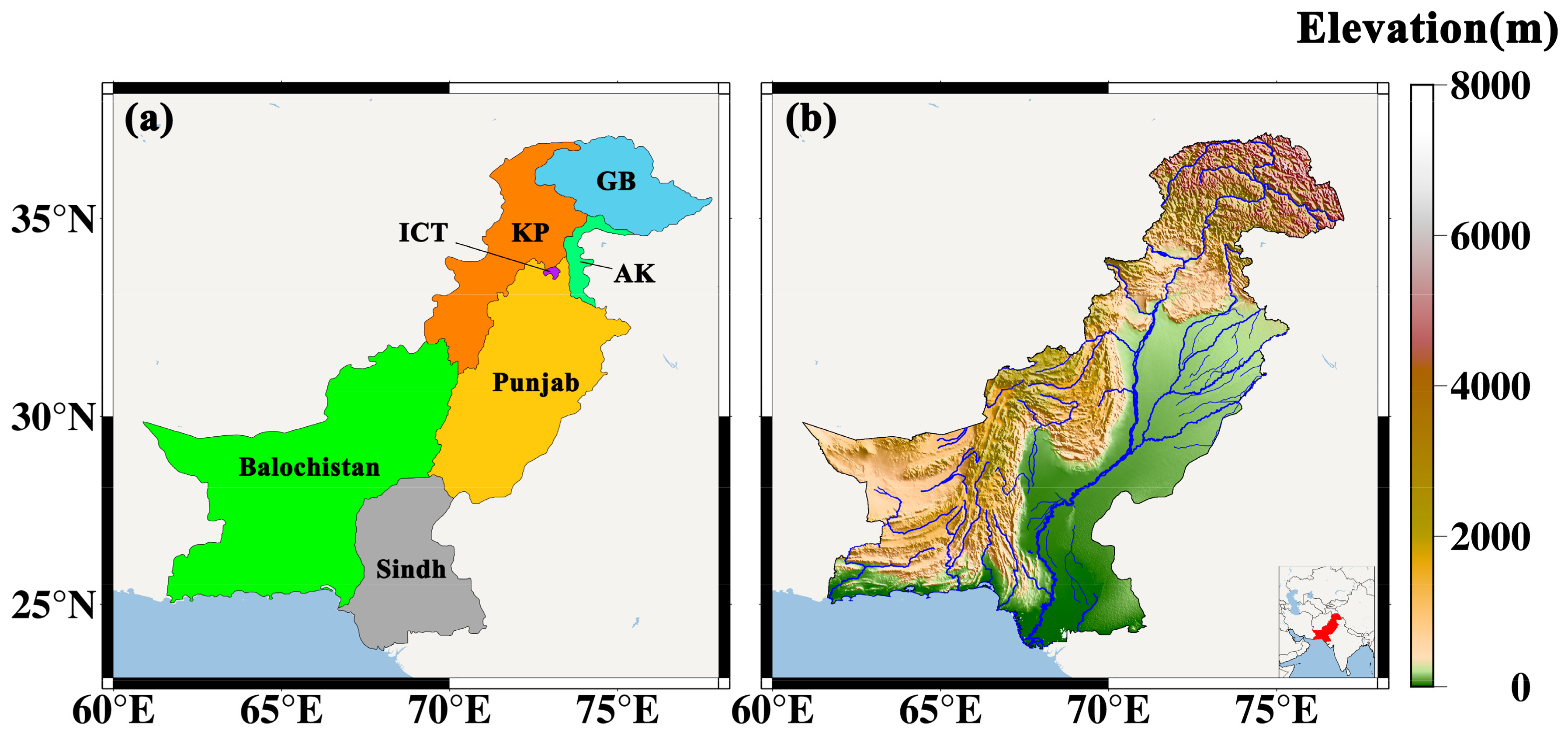
Figure 1. The administrative division (a) and topographic (b) map of Pakistan.
Remotesensing 16 01601 g001
Figure 2. The study flowchart.
Remotesensing 16 01601 g002
Figure 3. The time series of four GRACE TWSC and fused results in Pakistan from 2003 to 2022.
Remotesensing 16 01601 g003
Figure 4. The time series of GRACE and Swarm TWSC results in Pakistan from 2014 to 2022.
Remotesensing 16 01601 g004
Figure 5. The spatial distribution of uncertainty of GRACE and Swarm TWSC results in Pakistan.
Remotesensing 16 01601 g005
Figure 6. The time series of detrended TWSC derived from GRACE/Swarm and GLDAS in Pakistan between 2003 and 2022.
Remotesensing 16 01601 g006
Figure 7. Temporal evolution of PPT and TWSC anomaly in Pakistan between 2003 and 2022. (a) TWSC and PPT anomalous; (b) GRACE-DSI and SPI. The red box indicates the time when the flood occurred.
Remotesensing 16 01601 g007
Figure 8. The spatiotemporal evolution of monthly SPI in Pakistan between April and September 2022.
Remotesensing 16 01601 g008
Figure 9. The spatiotemporal evolution of monthly GRACE-DSI in Pakistan between July and November 2022.
Remotesensing 16 01601 g009
Figure 10. The center of gravity of flood movement trajectory maps. (a) 1–3 indicate from June to August 2022; (b) 1–6 indicate from July to December 2022. The blue arrows indicate the direction of the centre of gravity shift.
Remotesensing 16 01601 g010
Figure 11. The temporal evolution of STI, ET anomaly, SPI, SSI, and GRACE-DSI in Pakistan between January and December 2022. (a) STI vs. SPI vs. SSI vs. GRACE-DSI vs. ET anomaly. The dashed line indicates SPI/SSI/STI/GRACE-DSI = 0.5 and −0.5, respectively; (b) SSI vs. GRACE-DSI vs. runoff anomaly. The dashed lines indicate SSI/GRACE-DSI = 0.5 and −0.5, respectively.
Remotesensing 16 01601 g011
Figure 12. The temporal evolution of Niño 3.4 index (a) and DMI (b) between 2017 and 2022. The red shaded areas represent El Niño; the blue shaded areas represent La Niña.
Remotesensing 16 01601 g012
Figure 13. The standardized anomaly of geopotential height at 500 hPa between May and August 2022. Solid black line represents the contours of geopotential height (unit: gpm); solid purple line: the 5880 gpm in the current month; solid green line: the climatological state of 5880 gpm for the same period over the last five years; the region enclosed by the solid red line is Pakistan.
Remotesensing 16 01601 g013
Figure 14. The spatial distribution of severity of agricultural flood (a) and cropland (b) in Pakistan. (b) Green region represents the cropland.
Remotesensing 16 01601 g014
Table 1. Summary of the datasets in our study.
DatasetShort NameTime SpanSpatial ResolutionTemporal ResolutionData Source
GRACE/GRACE-FO SHCSR2003–20221° × 1°Monthlyhttp://icgem.gfz-potsdam.de/home, accessed on 10 November 2023
GFZ
JPL
GRACE/GRACE-FO MasconCSR2003–20220.25° × 0.25°Monthlyhttps://www2.csr.utexas.edu/grace/RL05_mascons.html, accessed on 10 November 2023
JPL0.5° × 0.5°https://grace.jpl.nasa.gov/data/get-data/, accessed on 10 November 2023
Swarm SH-2014–20221° × 1°Monthlyhttp://icgem.gfz-potsdam.de/home,
accessed on 10 November 2023
PPTERA52003–20220.1° × 0.1°Monthlyhttps://cds.climate.copernicus.eu/cdsapp#!/search?type=dataset, accessed on 10 November 2023
TEM
Runoff
SM
ETGLEAM 3.7a2003–20220.25° × 0.25°Monthlyhttps://www.gleam.eu/, accessed on 10 November 2023
SMGLDAS2003–20221° × 1°Monthlyhttps://disc.gsfc.nasa.gov/datasets?keywords=GLDAS_NOAH025_M_2.1&page=1, accessed on 10 November 2023
SWE
PCW
Land cover typeMODIS20220.05° × 0.05°Yearlyhttps://modis.gsfc.nasa.gov/data/dataprod/mod12.php, accessed on 10 November 2023
Niño3.4 indexENSO2003–2022-Monthlyhttps://www.cpc.ncep.noaa.gov/data/indices/, accessed on 10 November 2023
DMIIOD2003–2022-Monthlyhttps://www.cpc.ncep.noaa.gov/data/indices/, accessed on 10 November 2023
Geopotential Height-2003–20222.5° × 2.5°Monthlyhttps://psl.noaa.gov/data/gridded/data.ncep.reanalysis2.html, accessed on 10 November 2023
Table 2. PPT surplus category by SPI.
CategoryDescriptionSPI
S4Extreme wetSPI ≥ 2.0
S3Severe wet1.5 ≤ SPI < 2.0
S2Moderate wet1.0 ≤ SPI < 1.5
S1Light wet0.5 ≤ SPI < 1.0
S0No wetSPI < 0.5
Table 3. Wet category according to GRACE-DSI.
CategoryDescriptionGRACE-DSI
W5Exceptional wetGRACE-DSI ≥ 2.0
W4Extreme wet1.6 ≤ GRACE-DSI < 2.0
W3Severe wet1.3 ≤ GRACE-DSI < 1.6
W2Moderate wet0.8 ≤ GRACE-DSI < 1.3
W1Light wet0.5 ≤ GRACE-DSI < 0.8
W0No wetGRACE-DSI < 0.5
Table 4. Long-term changes trend and seasonal variation in GRACE and Swarm TWSCs in Pakistan.
TWSCLong-Term Change TrendAnnual AmplitudeAnnual Phase
GRACE−0.39 ± 0.35 mm/a0.25 cm−1.35 rad
Swarm−0.35 ± 0.30 mm/a0.33 cm−1.78 rad
Table 5. Meteorological flood characterization parameters in Pakistan.
RegionDuration (Months)PeakSeverityMax FAR
Balochistan2 (Jul to Aug)2.354 (Jul)3.83299.84% (Jul)
Sindh2 (Jul to Aug)1.994 (Jul)3.44199.59% (Jul and Aug)
Punjab2 (Jun to Jul)1.005 (Jun)1.562100.00% (Jun)
KP2 (Jun to Jul)1.806 (Jul)2.59998.15% (Jul)
GB3 (Jun to Aug)1.088 (Aug)3.11584.15% (Jun)
Table 6. Hydrological flood characterization parameters in Pakistan.
RegionDuration (Months)PeakSeverityMax FAR
Balochistan5 (Aug to Dec)2.305 (Aug)10.187100.00% (Aug to Sep)
Sindh6 (Jul to Dec)2.518 (Aug)12.139100.00% (Aug to Dec)
Punjab5 (Aug to Dec)1.063 (Aug)4.74775.00% (Nov)
Disclaimer/Publisher’s Note: The statements, opinions and data contained in all publications are solely those of the individual author(s) and contributor(s) and not of MDPI and/or the editor(s). MDPI and/or the editor(s) disclaim responsibility for any injury to people or property resulting from any ideas, methods, instructions or products referred to in the content.