Article

Remote Quantification of Soil Organic Carbon: Role of Topography in the Intra-Field Distribution

by
Benjamin J. Cutting
1,*,
Clement Atzberger
2,
Asa Gholizadeh
3,
David A. Robinson
4,
Jorge Mendoza-Ulloa
5 and
Belen Marti-Cardona
1
1
Department of Civil and Environmental Engineering, University of Surrey, Guildford GU2 7XH, UK
2
Institute of Geomatics, University of Natural Resources and Life Sciences, Vienna, Peter-Jordan Strasse 82, 1190 Vienna, Austria
3
Department of Soil Science and Soil Protection, Faculty of Agrobiology, Food and Natural Resources, Czech University of Life Sciences Prague, Kamýcká 129, 16500 Prague, Czech Republic
4
UK Centre for Ecology and Hydrology, Environment Centre Wales, Deiniol Road, Bangor LL57 2UW, UK
5
National Infrastructure Laboratory, Engineering and Physical Sciences, University of Southampton, Boldrewood Campus, Southampton SO16 7PP, UK
*
Author to whom correspondence should be addressed.
Remote Sens. 2024, 16(9), 1510; https://doi.org/10.3390/rs16091510
Submission received: 6 March 2024 / Revised: 22 April 2024 / Accepted: 23 April 2024 / Published: 25 April 2024
(This article belongs to the Section Environmental Remote Sensing)

Abstract

:
Soil organic carbon (SOC) measurements are an indicator of soil health and an important parameter for the study of land-atmosphere carbon fluxes. Field sampling provides precise measurements at the sample location but entails high costs and cannot provide detailed maps unless the sampling density is very high. Remote sensing offers the possibility to quantify SOC over large areas in a cost-effective way. As a result, numerous studies have sought to quantify SOC using Earth observation data with a focus on inter-field or regional distributions. This study took a different angle and aimed to map the spatial distribution of SOC at the intra-field scale, since this distribution provides important insights into the biophysiochemical processes involved in the retention of SOC. Instead of solely using spectral measurements to quantify SOC, topographic and spectral features act as predictor variables. The necessary data on study fields in South-East England was acquired through a detailed SOC sampling campaign, including a LiDAR survey flight. Multi-spectral Sentinel-2 data of the study fields were acquired for the exact day of the sampling campaign, and for an interval of 18 months before and after this date. Random Forest (RF) and Support Vector Regression (SVR) models were trained and tested on the spectral and topographical data of the fields to predict the observed SOC values. Five different sets of model predictors were assessed, by using independently and in combination, single and multidate spectral data, and topographical features for the SOC sampling points. Both, RF and SVR models performed best when trained on multi-temporal Sentinel-2 data together with topographic features, achieving validation root-mean-square errors (RMSEs) of 0.29% and 0.23% SOC, respectively. These RMSEs are competitive when compared with those found in the literature for similar models. The topographic wetness index (TWI) exhibited the highest permutation importance for virtually all models. Given that farming practices within each field are the same, this result suggests an important role of soil moisture in SOC retention. Contrary to findings in dryer climates or in studies encompassing larger areas, TWI was negatively related to SOC levels in the study fields, suggesting a different role of soil wetness in the SOC storage in climates characterized by excess rainfall and poorly drained soils.

1. Introduction

Soil organic matter (SOM) represents the major terrestrial store of soil organic carbon (SOC), but global stocks can only be estimated with high uncertainty [1]. The SOC content is an important indicator of soil health and fertility as its presence regulates nutrient provisioning, moisture of soil health, and fertility [2].
In addition to its implications for soil health and sustainable food production, SOC has a profound role in land-atmosphere carbon fluxes [3]. Indeed, the combined uptakes of both terrestrial and oceanic carbon sinks sequester over half of all anthropogenic emissions where the terrestrial reservoir alone accounts for a mass three times larger than current levels of atmospheric carbon [4,5].
Changes in SOC depend largely on land use, climate, agricultural management, and topography [6]. Intensive farming where little biomass is left over for incorporation into the soil, combined with high tillage intensities, induces SOC loss, thereby impacting soil health and promoting net positive emissions [7]. In contrast, well-implemented regenerative agriculture such as conservation tillage or crop residue retention, can enhance the organic carbon storage in soils. In order to promote regenerative agriculture and emission offsetting, the carbon credit market rewards farmers who adopt these practices. However, this market is currently hindered by a lack of objective, transparent, and cost-effective ways to monitor, report, and verify (MRV) the effectiveness of such regeneration practices [8].
Earth observation (EO) systems measure the radiation reflected or emitted by the Earth’s surface in different spectral bands. Given the strong absorption of SOC in the optical domain (wavelengths from 350 to 2500 nm [9,10]) several studies have attempted to measure and map SOC content in the topsoil using EO data from various platforms such as satellites, piloted aircraft, and unmanned airborne vehicles (UAVs, [11,12,13]).
The use of satellite platforms such as Sentinel-2 provides periodic, consistent, and cost-effective observations over large areas which would be unfeasible for aircraft [14]. Satellite periodicity is of particularly high importance as it facilitates the use of multidate images with a high temporal resolution, enabling potential improvement in model performance while minimizing cloud issues [15]. While the use of airborne hyperspectral data typically outperforms spaceborne sensors as more details in the spectral signatures can be resolved [16], clear limitations are apparent such as limited availability and relatively high cost. Of those studies utilising spaceborne data, the use of Sentinel-2 is very common having been shown to often outperform comparable platforms such as Landsat-8. This is likely due to its higher spatial resolution in the visible and NIR range, greater temporal resolution, and the inclusion of the red edge bands. The commonality of Sentinel-2 in remote sensing also facilitates a more apt comparison between this study and the literature. While the aforementioned studies demonstrate that EO spectral measurements provide quantitative information on SOC [10], some studies have shown that the incorporation of topographical features such as terrain elevation or topographical wetness index (TWI, [17]) can improve the SOC predictions [13,18]. Topography is closely related to the movement and accumulation of water and material across the landscape and, consequently, contributes to SOC distribution. The use of TWI in larger studies typically exhibits a positive correlation with SOC [19,20,21,22,23,24]. This is theorised to be due to erosion and/or overland flow which transport SOC over large distances [21]. Furthermore, water accumulation can induce anaerobic conditions, decreasing the decomposition rate of SOC. However, the use of topographic covariates, especially with regard to soil moisture, lacks research on smaller, crop field scales where microtopography becomes important. Therefore, the study of topographical covariates over, smaller, intra-field scales is vital and complimentary to the analysis of larger field sites with low sampling densities.
Many studies have demonstrated the efficacy of using multitemporal data in ML models [13,25,26,27]. The use of multidate imagery helps smooth the effects of single-date spectral anomalies and reduce the effects of spectrally active dynamic variables which do not exhibit covariance with SOC. Moreover, Vaudour et al. suggest that, although the use of multitemporal data does not guarantee improved performance, its use does improve generalisability [28]. No study to date has incorporated a comparison of multitemporal data and topography at smaller crop intra-field scales to study scalability for small areas at high resolution.
The objectives of the study presented here were to: (1) assess the capability of single and multidate Sentinel-2 spectral data for quantifying the spatial distribution of SOC within crop fields, using common models such as Random Forest and Support Vector Regression; (2) to assess if the conjunctive use of spectral data with topographical features improved the SOC prediction accuracy; (3) to assess the importance of different predictors. These objectives are motivated by the aim to better understand processes related to organic carbon conservation in the soil and their relationship to soil moisture at smaller, high resolution scales. To permit the analysis of these objectives, an intensive field campaign was conducted within an agricultural site in Southeast England owned by the University of Surrey. The site has 30 years of recorded farming practices which suggested a large range of SOC values and thereby potentially improving model validation.

2. Study Area

The study area consists of three crop fields located in the county of Surrey, in the Southeast of the United Kingdom (UK), extending across 51°13′42.7″ to 51°14′17.0″ North latitude and 0°37′40.6″ to 0°38′19.8″ West longitude (WGS84 datum). The fields are labelled F1, F2 and F3 in Figure 1 and have areas of approximately 10, 5, and 2.5 hectares, respectively. These fields have been regularly farmed for over three decades. Oat was the crop grown on the three fields from October 2020 till August 2021, before our sampling campaign in September 2021.
F1 has shallow calcareous silty soils characterised by the Upton series [29] (grey rendzinas), with thickness varying from 0.25 m to 0.75 m depth. The northern end of F1, and fields F2, F3 contain poorly draining loamy and fine silty soils over clay primarily in the Wickham 4 association (typical stagnogley) [30]. A soil survey commissioned by the farmer in 2014 (personal communication) confirmed this general soil description. This survey also pointed at higher SOC content in field F3, presumably due to cows from an old dairy farm having pastured in it. A nearby abandoned stable was observed during the site work.

3. Materials and Methods

The soil sampling campaign and a UAV survey flight were conducted simultaneously over the study fields on the 7–8 September 2021. The three study fields had been harvested between the 25–26 of August.

3.1. Onsite Sampling

Samples were acquired at 55 locations distributed over the study fields as shown in Figure 1. The sampling locations were planned so that their spatial distribution was approximately uniform, while capturing subtle spatial anomalies observed in the long-term average (2017–2021) of Normalised Difference Vegetation Index (NDVI). The resulting average spatial density (55 samples over 17.5 ha) clearly exceeded those found in the literature of SOC remote sensing.
Soil samples representative of the top 10cm soil layer were collected at different points randomly distributed within a 2.0 m × 2.0 m plot. This sampling depth is recommended in the UK Farm Toolkit [31]. Crop residue and stones were carefully excluded from the soil samples, which were then introduced into a plastic bag per sampling point, labelled and immediately stored in a cool, dark container. The sample bags were deposited in a dark laboratory refrigerator at the end of each sampling day and kept there until the SOC analysis was conducted.
For all locations, the square sampling plots of 2.0 m × 2.0 m with North-South orientation were defined. This extent is consistent with that used in the Countryside Survey: Soil Report from 1998 and 2007 [32]. A small white-clay mark was placed at the south-eastern corner of each sampling plot. The very-high-resolution UAV imagery acquired during the survey flight was used to identify and extract the coordinates of the clay marks (i.e., sampling points) with a 0.05 m accuracy (see Section 3.5 for survey details). It is worth noting that the marks were placed right after the Sentinel-2 overpass, to avoid any impact on the satellite spectral measurements.

3.2. Laboratory Analysis of Soil Organic Carbon

Soil samples were analysed at the University of Surrey Advanced Geotechnical Engineering Laboratory for organic matter and soil texture. The raw samples, with mass ranging between 400 g and 700 g, were air-dried overnight to allow for manual disaggregation of soil clumps and passed through a 2 mm sieve. They were then mixed and divided by Cone Quartering (British Standards Institute [33]) until subsamples of approximately 10 g were obtained.
The organic matter content of the sub-samples was determined using the Loss-on-ignition method [11,34]. Two subsamples from each sampling point were used to calculate the organic matter. The air-dried sub-samples were placed on a dry alumina crucible of known dry mass and oven dried at 105 °C for 24 h. They were later cooled to room temperature inside a silica gel dissector to ensure that moisture did not contaminate the sample. The dry mass of the subsamples was measured to an accuracy of 0.1 mg and then kept in a furnace at 375 °C for 16 h to induce the combustion of the organic matter [35]. This temperature is lower than the 400 °C reported in other studies to prevent the CO2 release from carbonates, as visible chalk fragments were present in some of the samples [36,37]. When taken out from the furnace, the subsamples were cooled down in a silica gel dissector and the dry mass measured to an accuracy of 0.1 mg. The percentage weight of SOC in the subsamples was calculated as follows
S O C = 55 w 105 w 375 w 105
where w 105 is the mass of the soil subsample after drying at 105 °C for 24 h (mg) and 375   ° C is the mass of the soil subsample after heating at 375 °C in the furnace for 16 h (mg). Equation (1) was adapted from SOM to SOC by multiplying by a factor of 0.55 [38].
The SOC percentages obtained for the two subsamples from each location were consistent in all cases, except for one which was resampled and reanalysed. After this reanalysis, SOC pairs of results differed by less than 0.2% in 80% of the locations, and by less than 0.4% for all of them. The sampling point’s SOC was calculated as the average of the pair of results.

3.3. Satellite Data, Image Pre-Processing and Indices Calculation

A cloud-free Sentinel-2 image of the study area was acquired on the 8 September 2021, coinciding with the soil acquisition campaign. The Sentinel-2 data was downloaded from the Copernicus open access hub as Level-2A bottom of atmosphere (BoA) reflectance product. Our analysis used the (10) Sentinel-2 bands (Table 1) considered sensitive to soil properties [39]. The nearest neighbour method was used for resampling all 20 m pixels to 10 m. Time series of cloud-free Level-2A BoA spectral reflectance were then extracted for each sampling point using the Google Earth Engine (GEE) platform. These Sentinel-2 spectral data were then imported into Python 3.11. This served as the environment in which further preprocessing and spectral index calculations were conducted.
To reduce the effects of non-linearity and scattering, the reflectance spectra were converted to apparent absorbance such that
A = ln 1 R
where R is the reflectance [41]. This is primarily due to the gaussian nature exhibited by both the actual and apparent absorbances [42].
From the spectral reflectance values, two spectral indices were initially calculated: the Normalised Difference Vegetation Index (NDVI) and the Normalised Burn Ratio (NBR2) [43,44]. NDVI and NBR2 are indicative, respectively, of the amount of photosynthetically active vegetation and crop residue present in a pixel. Pixels with values higher than 0.2 for these indices were excluded from the analysis as their vegetation or crop residue coverage could hinder the spectral response of the soil This left roughly 40 pixels remaining to be analysed.
In addition to the above, other spectral indices were calculated, as their use has been shown to improve the modelling of SOC [45]. Table 2 summarizes these indices.
In addition to using a single-date Sentinel-2 image, a multi-temporal approach was also assessed, where average (median) spectral signatures were used as predictor variables. Multi-temporal data has the advantage of being largely unaffected by single date spectral anomalies and, moreover, is resistant to the effects of dynamic variables such as surface moisture and roughness which have no correlation with SOC. Cloud-free Sentinel-2 images acquired up to 18 months before and after the soil sampling campaign data (7th and 8th of September 2021) were collected. The 18 month period either side of the sampling date was chosen because the SOC change due to agricultural practices over this time span is expected to be clearly below the detection threshold of spectral methods [57]. Over the 1.5 year window, the maximum change would be lower than 0.08% SOC, which is below the RMSE of remote sensing based SOC models [58]. Hence, the SOC measurements should still be related to the spectral data acquired less than 18 months apart.

3.4. Extraction of Topographical Features

A terrain elevation point cloud of fields F1, F2 and F3 was acquired using the Headwall Photonics hyperspectral and LiDAR sensor (Bolton, MA, USA), mounted on a DJI M600 Pro UAV and operated by the Field Spectroscopy Facility (FSF) of the UK Natural Environment Research Council (NERC). The UAV flight was conducted on the 7th and 8th of September 2021, concomitantly with the soil sampling campaign, between 10:00 and 14:00 solar time at 120 m height above ground. A GPS base station was used to convert the UAV GPS records to post-processed kinematic (PPK) coordinates with 0.05 m accuracy. The LiDAR measurements were filtered for atmospheric artefacts (e.g., dust) and a point cloud for the overflown areas was produced at PPK geospatial accuracy. The cloud was converted into a digital elevation model (DEM) in raster format at 0.05 m spatial resolution for the orthorectification of the hyperspectral data by NERC-FSF using own software. The later was used for the visual identification of the sampling point marks (see Section 3.1). Unfortunately, the hyperspectral measurements presented some radiometric inaccuracies that invalidated their use as SOC predictors.
The LiDAR point cloud was also used to produce a 1m-resolution raster DEM using the Envi 5.8 software and used to extract the topographical features of the study fields at the location of each soil sampling point (coded in Python 3.11). These features included relative terrain elevation, drainage path length, local surface gradient, curvature, convexity, aspect, and topographical wetness index (TWI). The relative elevation was calculated for each field by subtracting the minimum field elevation. The surface gradient was calculated as the maximum slope in the eight directions of a 9 × 9 DEM window centred at each pixel. Hurst et al. [59] found that fitting a 6-degree polynomial surface to a nine-by-nine window was apt for estimating the curvature of the surface. This was used to calculate the minimum and maximum curvature at each sampling point and the convexity.
The drainage path length of each sampling point represents the distance along the steepest gradient line from the sampling point to the highest upper end of the field. This length is indicative of the amount of runoff that reaches the point during and after a rainfall event. This path length was measured by performing gradient ascent from each respective pixel until the upper field boundary, assumed to impede runoff from upstream surfaces. Finally, the TWI is defined for a point p as:
T W I p = ln A s p tan β p
where A s p and tan β p are the specific catchment area and the slope at a given point p , respectively. The specific catchment is the upslope area draining through a point per unit contour length. For approximately planar fields, as F1, F2 and F3, the area per unit length becomes constant and equal to the drainage path length, L , so TWI can be expressed as
T W I ln L tan β .
Expression (4) was used to calculate TWI at the sampling points. These topographical parameters could then be used simultaneously with the spectral metrics with the aim of improving model performance. Of the larger set of topographical covariates, it was decided that redundant variables and those with poor correlation be removed for model clarity (See Section 3.8).

3.5. Machine Learning Models for SOC Prediction

Random Forest (RF) and Support Vector Regression (SVR) algorithms, with a radial basis function kernel for the latter, were trained, tested, and validated to predict SOC using Sentinel-2 spectral data, topographical data, and a combination of both data types. Both RF and SVR were implemented using the Scikit package in Python 3.11 [60].
The data set was partitioned such that 80% formed the training set for the model, and the remaining 20% a validation or testing set. All the predictors were normalised for the training set such that the population mean equalled zero and the standard deviation equalled one. This was necessary due to both the Gaussian assumption inherent in SVR as well as the large differences in the value ranges between spectral bands. The training set could then be used to optimise the models. To permit a better comparison with previous studies [12,61,62,63], an RBF kernel was selected for the SVR model [12,61,62,63]. Moreover, RBF is a common choice as it exhibits isotropy, is stationary, and has fewer tuning parameters making it is easier to apply for complicated non-linear systems.

3.6. Random Forest

RF involves the generation of a large collection of decision trees commonly referred to as a ‘forest’ [64]. A given decision tree normally uses a subset of the available features in the dataset. The first node is then created by generating a given number of randomly generated inequalities where any given statement splits the dataset in one dimension of the multidimensional feature space. The inequality is then selected which results in the greatest reduction in the total variance of the system. This process is then repeated to build the decision tree until a given variance threshold is achieved. Upon completion, a highly specified decision tree has been generated capable of sorting the data although said tree is highly likely to be an example of overfitting. By generating a collection of trees in the same fashion, each using a different feature subset, the overfitting of the decision trees is reduced. The RF hyperparameters are specified in Table 3.

3.7. Support Vector Machine

SVR (with a radial basis function) attempts to minimise the sum of the squared differences between observed and predicted values subject to a constraint whereby a proportion of the points have to be within a given squared difference threshold value, ε. The algorithm, therefore, can be imagined as generating a series of regression lines in a space with as many dimensions as model’s predictors. The observed SOC can be represented as points in the same space. The regression lines are iteratively refined to achieve the overall least sum of squared differences between observed SOC values and corresponding predictions in the regression line, while containing the largest proportion of observation points within a threshold distance, ε, of the regression line. The hyperparameters for this algorithm are specified in Table 3.

3.8. Model Assessment and Optimisation

In total, 5 different feature sets were analysed to quantify the spatial distribution of SOC within crop fields (Table 4): (1) single date Sentinel-2 spectral data, multidate Sentinel-2 spectral data, and topographical covariates independently; (2) a conjunction of topographical covariates with single-date and multidate spectral data, respectively. It was decided that, to improve model performance and importance analysis, highly autocorrelated and redundant topographic variables would be removed to form an ‘optimum’ subset. We defined redundant variables such that their removal from the model resulted in no change or even an improvement in model performance.
To determine the optimal hyperparameters for the SVR and RF models, the Multiobjective Tree-structured Parzen Estimator (MOTPE) was used through the Python package Optuna [65]. This method utilises 5-fold cross-validation (CV) to determine the root-mean-square error (RMSE) at given points in the hyperparameter space. Although k can be any integer greater than zero, 5 or 10 are common values picked in remote sensing studies [61,66,67,68,69]. As a 10-fold CV would have been inappropriate with only 5 to 6 points in each fold, a 5-fold CV was chosen. CV also outputted the R 2 and the mean absolute error (MAE) as further metrics to monitor model performance. These metrics are such that
R M S E = i = 1 n y i y ^ i 2 n
R 2 = 1 i = 1 n y i y ^ i 2 i = 1 n y i y ¯ 2
M A E = i = 1 n y i y ^ i n
where n is the total number of points, y is the set of ‘true’ or observed values, y ^ is the set of predicted values, and y ¯ is the mean of the y .
Using the CV metrics, the algorithm seeks to maximise the probability density function
p x = x ,         Y < Y * g x ,         Y Y *  
where Y is a given observation, x is a vector of hyperparameters, and Y * is the point that maximises the function. As a form of Bayesian optimisation, MOTPE requires an acquisition function to establish a global optimum. MOTPE utilises Expected Improvement (EI) to select the optimum model for each iteration. By applying EI to our probability function (8), it can be shown that points with a high probability of model improvement become separated from those with a low probability, allowing the algorithm to converge toward the optimum hyperparameters in fewer iterations than would be achieved by other popular methods such as grid search. After N iterations, the hyperparameters of the most successful model are extracted and used to fit the training data. The model in question now performs well when predicting data it has been trained with.
While a combination of Bayesian optimisation and CV reduce model overfitting, it should be noted that achieving an approximately optimal CV error does not fully eliminate the possibility of overfitting. Therefore, to validate the model, it is necessary to split the total dataset into training and validation sets as mentioned prior. The ‘optimum’ model achieved via Bayesian optimisation is then tested on the individual and independent validation set. From this, the validation RMSE, R 2 , and MAE are calculated so as to assess the accuracy of the model. Therefore, overfitting can be identified accurately: a low CV error contrasted by a high validation error suggests as such.
In addition to these metrics, models exhibiting higher accuracy were used to extrapolate and predict the SOC content over the entire field set and, in this way, analyse the associated spatial distribution of SOC prediction. To achieve this, topographic and spectral data were inputted for each respective pixel forming rasters of SOC prediction. From these data, coherent maps could then be generated using the Python packages Cartopy 0.23 and Salem 0.3.09 [70,71].

3.9. Variable Importance Analysis

To evaluate the relative importance of each input variable with regard to the model’s accuracy, permutation feature importance was used from the Python package Scikit [60]. As developed by Breiman, permutation importance starts by computing a reference score based on the standard permutation of input variables [72]. Then, for each variable, the values are randomly shuffled such that a given input variable is now given in the place of another. For example, B2 absorption might be inputted in place of B3 and vice vera. The score of this new permuted dataset is calculated for a particular feature and subbed into
i j = s 1 K k = 1 K s k , j
where s is the baseline score, K is the total number of repetitions, and s is the shuffled score for some given permutation. While permutation importance is still a local property and thus cannot predict intrinsic value, it is resistant to the effects of variables with high cardinality. Therefore, said metric will be used as indication of relative importance of input variables.

4. Results

4.1. SOC Analysis of the Soil Samples

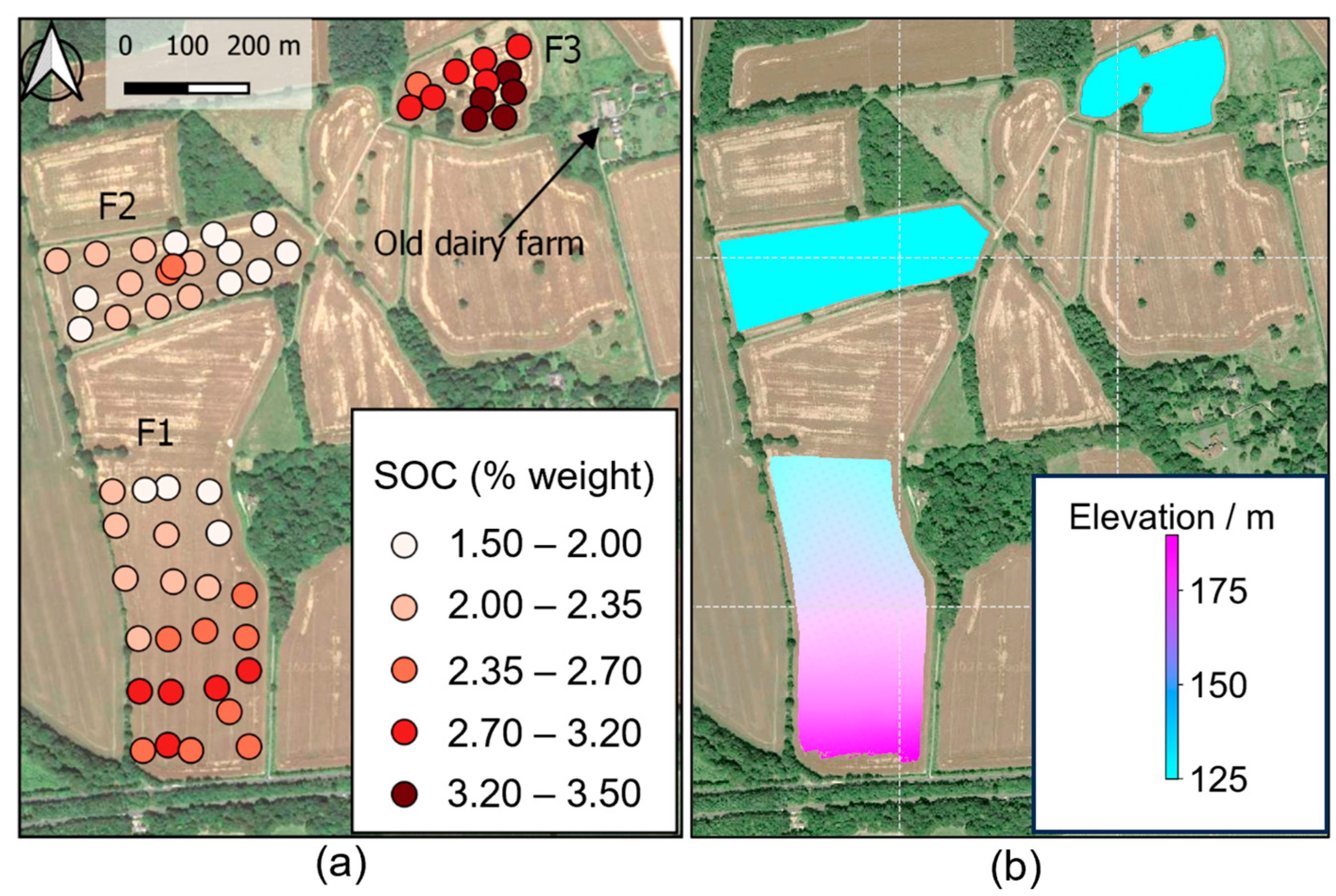
Figure 2 depicts the SOC laboratory measurements at their respective sampling locations and the elevation measurements collected from the UAV flight. The SOC values vary from ~1.5% to ~3.5% in fields F1 and F2 with values above 3% for most samples of F3. Field F1 shows higher SOC content in the southern half, coinciding with an area of chalk substrate where the soil is better drained. The higher SOC concentrations in F3 are due presumably to the fact that cows used to pasture on the field. Therefore, the study site has a relatively varied distribution of SOC values. Details of SOC statistics can be found in Table 5.

4.2. SOC Model Performance for SVR and RF

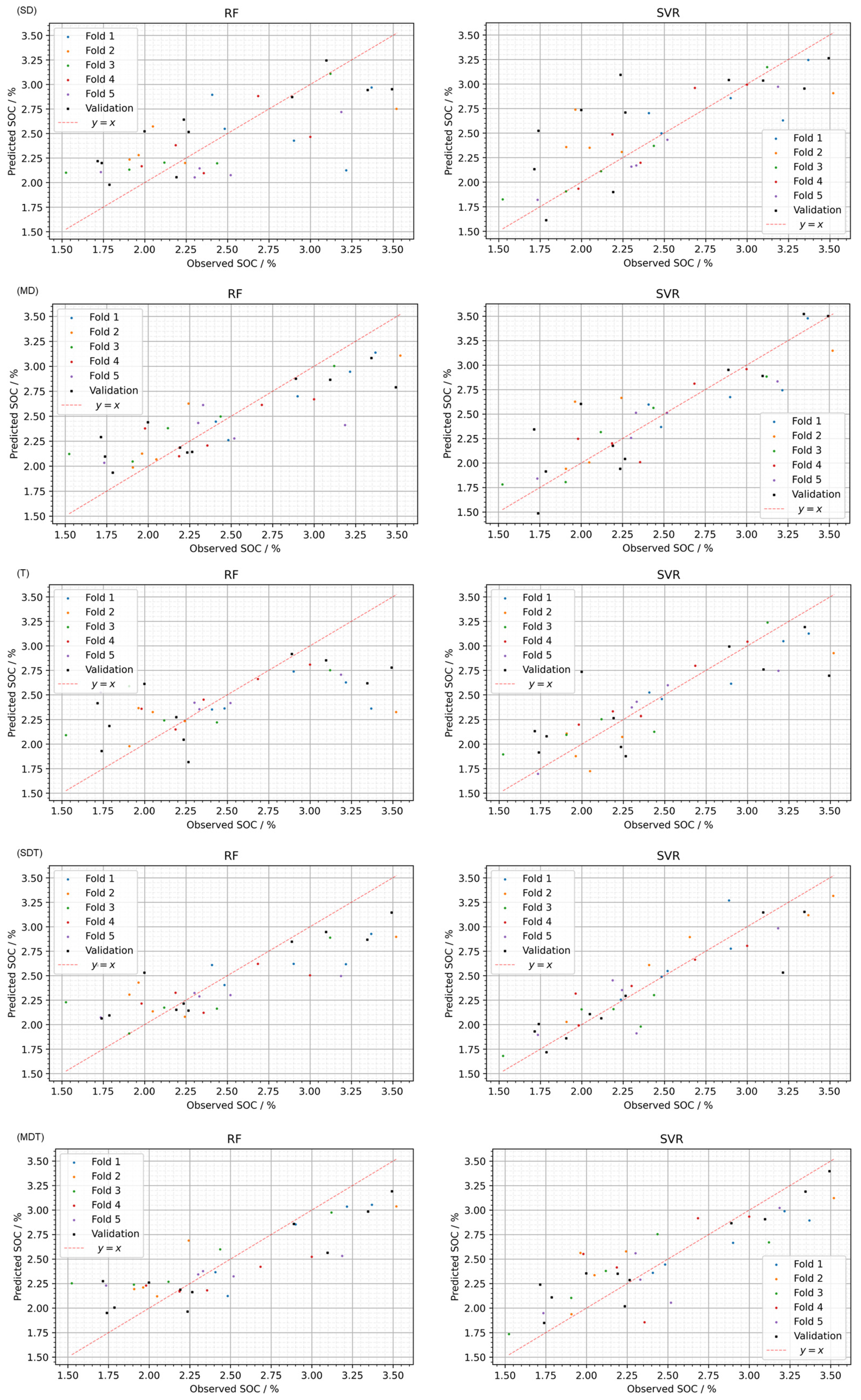
Using the different combinations of the input data, 5 models were formed for SVR and RF (Table 4—above). The performance of these models in summarised in Table 6. For SD, the CV-RMSEs were found to be 0.42% and 0.30% for RF and SVR, respectively. The uncertainties inherent to both suggest there is a significant difference between the CV errors attained for both models with regard to RMSE and R2 but not MAE. On the other hand, the validation RMSEs were found to be 0.47% and 0.53% for RF and SVR, respectively. Therefore, contrary to the CV metrics, RF performed better although both values are relatively poor. Figure 3a provides a detailed visual comparison of the performance of each model by plotting the observed values vs those predicted by the model. The circular points represent the five folds used in CV while the black indicate the predictions on the validation set. A ‘perfect’ model would only occupy the y = x line.
The use of temporal data, In MD as opposed to single-date resulted in CV-RMSEs of 0.35% and 0.32% for RF and SVR, respectively. While significant improvement is only noted in the CV-RMSE of RF between SD and MD, the validation metrics of both models improve significantly between with RMSEs of 0.34% and 0.31% for RF and SVR, respectively.
It was necessary to train both models using just the topographic variables so as to ensure the models are not ‘guided’ by these features alone. If this were the case, Sentinel-2 data would be obsolete for determining SOC levels and confirm a lack of temporal transferability. Model T in Table 6 summarises the performance statistics (R2, RMSE, and MAE) for all assessed models when using just the topographic variables and scatter plots for both. RF performs worse than the combined model and is comparable to the model trained on Sentinel-2 data alone. This is true of both the CV error and the validation error. For SVR, the CV error is the lowest of any of three single-date models. However, the validation error is significantly worse than the combined model, implying overfitting when using the topographical variables alone.
It was found that the introduction of topographical data to models using Sentinel-2 spectral data (model SDT), greatly improved the models’ SOC predictions. However, as mentioned in Section 3.8, there was redundancy and autocorrelation in the contribution of the topographical features, and the subset of them providing the best predictions was found to be: relative elevation, TWI, and slope. Therefore, curvature, aspect, and convexity served only to reduce model performance or obscure importance metrics. Model SDT achieved CV-RMSEs of 0.33% and 0.27% for SVR and RF, respectively. Both models see an improvement in the mean CV metrics and a reduction in the associated uncertainties although there is no significant difference noted between the two models with the exception of the CV-RMSE for the RF model. In spite of this, the validation RMSEs are 0.395% and 0.283% for RF and SVR, respectively. Therefore, both experience improvement with SVR performing best. Figure 3d shows the CV and validation predictions from both models.
Finally, MDT was found to produce CV-RMSEs of 0.34% and 0.33%, respectively. While these values represent no significant difference between those in the SDT, both algorithms exhibited their best validation performance with RMSEs of 0.29% and 0.23%, respectively. Therefore, SVR for MDT resulted in the greatest validation performance of any of the models generated.

4.3. Permutation Importance

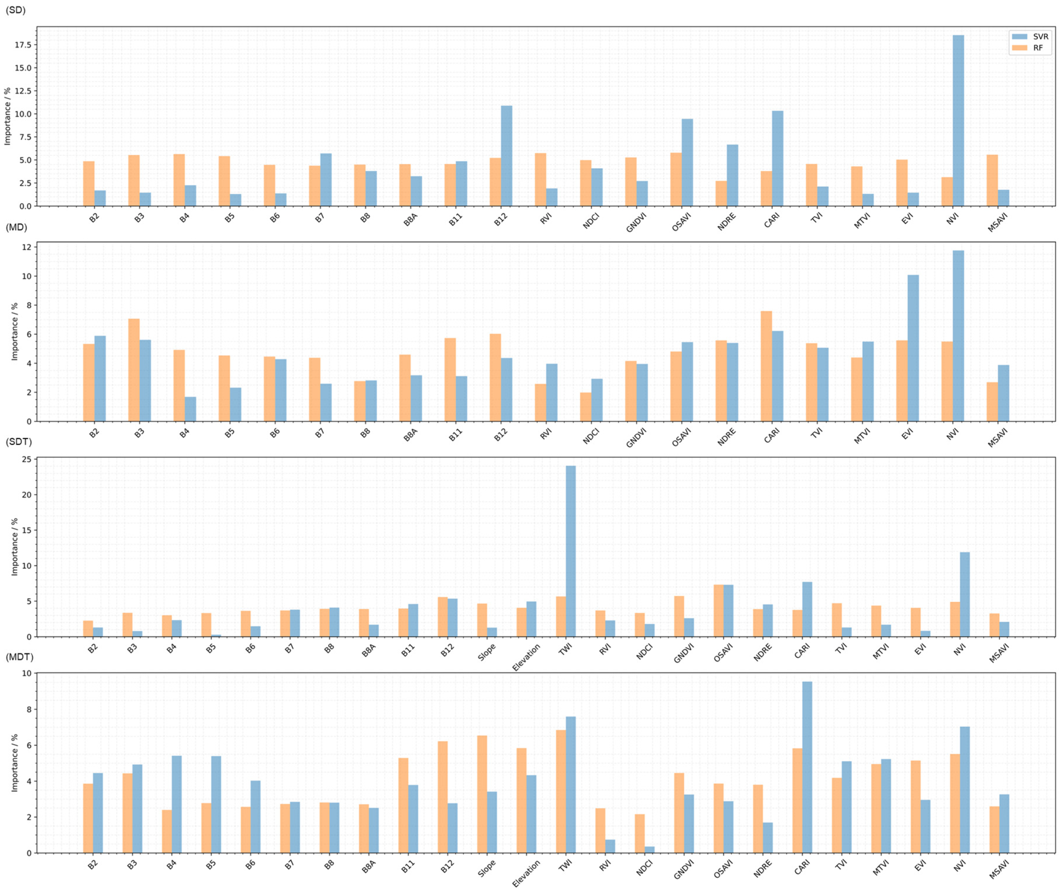
Figure 4 gives the permutation importance for each of the respective models with the exception of model using topographic covariates alone. Each figure label aligns to its respective model. In SD, SVR attributes importance to a small subset of variables with NVI being the most important while RF exhibits a largely even spread of importance across all features. For model MD, both algorithms exhibit largely similar values to SD although with minor increase in band importance. For SDT, it is evident that the SVR model likely has a high reliance on a smaller subset of features. Clearly, both algorithms indicate that TWI is important for performance. Finally, RF for MDT showed consistency with the single-date importance having a similar distribution of importance which improves our veracity in the algorithm. On the other hand, SVR attributed high importance to the visible bands and, in contrast to the single-date models including topography, although still attributed a high importance to TWI.

4.4. Model Extrapolation over Sample Area

To evaluate the spatial SOC predictions of the models in question, spectral and topographical raster were input into models MD and MDT respectively, generating SOC prediction heatmaps over the extent of F1, F2, and F3. Figure 5a shows the maps for both SVR models. It is clear that the introduction of topographic features creates a smoother distribution of SOC prediction. Figure 5b demonstrates the same effect but for the RF models.

5. Discussion

Our results, depicted in Figure 3, indicate that both RF and SVR models perform aptly in their CV prediction of SOC for Sentinel-2 data taken on an intra-field scale. The obtained CV accuracy, which yielded an RMSE between 0.42% and 0.27% and the validation accuracy, with an RMSE of between 0.53% and 0.23%, is consistent with that reported in similar studies reviewed by Lamichhane et al. [73]. Contrary to Latmichhane et al., our analysis, however, found that SVR largely outperformed the equivalent RF models. This does not represent an inherent contradiction as they note that RF continued to perform well for smaller sample sizes but typically over large, diverse areas. Therefore, the intra-field scale combined with a smaller sample size may favour SVR. Indeed, RF is a bootstrap process and so can experience performance issues due to repetition for smaller sample sizes. Moreover, Zhou et al. suggest that no single predictive model attains peak performance for every circumstance, supporting the validity of our results [26]. On a more cautionary note, the best performing single-date models were poorer in the context of some other contemporaneous studies [45,74,75]. However, it is suggested that said studies differ sufficiently from this study that the performance achieved remains comparably competitive. For example, Yang et al. employed a 250m resolution grid of soil properties. This was the most important variable in their model and is therefore most likely to account for the improved performance [75] multi-date (MD) and multi-date + topography (MDT) models showed improvement in validation performance over their single-date counterparts although the latter showed no significant difference when comparing the CV error. This improvement is to be expected as the temporal averaging contributes to reinforce the spectral contribution of the soil inherent optical properties, such as SOC, while reducing noise [13,15,18,26]. In our research, the use of multitemporal data was found to improve model performance, for both RF and SVR, on an intra-field scale.
The introduction of topographical covariates exhibited clear improvements in performance for both the single-date and multitemporal counterparts. The validation errors of these conjunctive models were significantly lower than those achieved for model using solely topographic features (T). Therefore, we assert that union of spectral data and topographical was advantageous to achieve optimum model performance. Of the topographical models, MDT was found to have the highest validation performance of any of the respective models with reductions in RMSE of 38% and 57% in comparison to SD. Therefore, based purely on validation RMSE, the multitemporal SVR model, including topographical features, had the best performance of any of the previously trained models. Moreover, this This value represented a significant difference to the mean value of similar studies appraised over the last 5 years [13,26,27,45,76]. In the case of RF, both the spectral bands and the covariates had comparable importance despite their inherent autocorrelation. On the other hand, SVR tended to attribute higher importance to a smaller subset of features. These did not necessarily corroborate one another though. For example, B12 was found to be important in the single-date spectral model. Castaldi et al. notes the importance of B12 for the detection of water and its sensitivity to vegetation. However, the reduction in importance for SVR in the multitemporal models suggests that the single-date importance, in this case, has little physical meaning. Overall, the four SVR models consistently attributed importance to NVI and, to a lesser extent, CARI and B12. NVI and CARI both use bands from the red to red-edge wavelengths. Gholizadeh et al. found that SOC had the highest correlations with Sentinel-2’s B4 and B5 bands (VIS region & red edge) while working on Chernozems and Cambisols with low levels of SOC (0.63/4–2.62%) [11,77,78]. Therefore, the importance of both NVI and CARI may be emergent from the sole input of wavelengths falling between the red and red-edge sections of the spectrum. NVI was also found to have relatively low correlation with other features and, therefore, high permutation importance could be due to the autocorrelation of the system and not any direct physical relation imparted by NVI.
Of the topographical features, TWI was found to have a consistently high importance in the SVR models. This was also true of RF although it was exhibited more clearly in MDT. Since TWI represents water accumulation by relief (Sena et al. [79]), performance appears improved by introducing knowledge of soil moisture likelihood. In contrast, de Almeida Minhoni et al. [13] found TWI to be a poor indicator of SOC and favoured elevation which, in this study, saw greater importance for RF models. Moreover, Li et al. [80] noted a strong positive correlation between TWI and SOC, theorising that high moisture leads to enhanced plant production and root biomass. We observe the opposite, with a negative trend between SOC and TWI. In our study fields, soil moisture is not a limiting factor for plant development. On the contrary, some areas are often water saturated. We therefore hypothesize that the excessive soil moisture could have led to poorer root development and lower inputs of plant biomass in general.

6. Conclusions

This study assessed the viability of mapping intra-field SOC distribution using Sentinel-2 spectral data. SOC was measured at 55 sampling locations over three study fields and used to train RF and SVR machine learning models. Five different sets of model predictors were assessed: the use of Sentinel-2 spectral measurements from a single-date (SD); multidate Sentinel-2 spectral measurements (MD); topographical data alone (T); the conjunctive use of the single-date Sentinel-2 data (SDT) and topographical data; the conjunctive use of topographical data and multitemporal satellite data (MDT).
We found that the models based exclusively on Sentinel-2 data showed slightly poorer performance than other similar ones in the literature. Contrary to other publications, our SVR model performed better than the RF one, with CV-RMSE of 0.47% and 0.30%, respectively. The relative importance analysis indicated that a spectral index combining the red and red edge bands (NVI) and B12 were the most informative predictors for SVR. The spread of importances exhibited by RF was such that no one feature could be said to be most informative with any significance.
By introducing topographical features, the SOC prediction improved both the CV and validation accuracies compared to the models based on single-data Sentinel-2 data only (SDT), resulting in validation RMSE reductions of 21% and 9% for RF and SVR, respectively. Similarly, RMSE validation reductions of 16% and 47% were observed between the purely topographic models and the conjunctive single-date models for RF and SVR, respectively, clearly demonstrating the usefulness of spectral data for predicting local SOC distributions which cannot be captured by topographical variables alone. SVR and RF attributed the highest permutation importances to, firstly, TWI and, secondly, NVI. Similar to the spectral models, RF had a more even spread of importances across all features whereas SVR relied more heavily on a smaller subset of bands.
The best performing models were achieved by using topographical features and multitemporal Sentinel-2 data, MDT, with a reduction in validation RMSE from the single-date spectral model of 38% and 52% for RF and SVR, respectively. The validation RMSE of 0.23% for SVR was found to be comparable or outperform those reported in similar studies. Although some disparity was observed in the relative importance of features, TWI consistently showed high relative importance for RF and SVR.
The SOC models SDT and MDT yielded similar CV accuracies of 0.33% and 0.34%, for RF and 0.27% and 0.33% for SVR, respectively. These results strongly highlight the relevance of topographical features and multitemporal spectral data for the high-resolution intra-field mapping of SOC. TWI emerged as a very relevant parameter for explaining intra-field differences in SOC, exhibiting negative correlation with SOC concentration, which could be potentially explained by the role of soil moisture in plant and root development.

Author Contributions

Conceptualization, B.J.C., B.M.-C. and C.A.; methodology, B.J.C., B.M.-C., A.G. and J.M.-U.; software, B.J.C.; validation, B.M.-C., C.A. and D.A.R.; formal analysis, B.J.C. and B.M.-C.; investigation, B.J.C., B.M.-C. and D.A.R.; data curation, B.M.-C., J.M.-U., A.G. and C.A.; writing—original draft preparation, B.M.-C., B.J.C. and A.G.; writing—review and editing, B.M.-C., B.J.C., C.A. and D.A.R.; visualization, B.J.C.; supervision, B.M.-C.; project administration, B.M.-C.; funding acquisition, B.M.-C. and C.A. All authors have read and agreed to the published version of the manuscript.

Funding

This study received financial support from UK Research and Innovation (UKRI) through the Space Research and Innovation Network for Technology (SPRINT) program, from Mantle Labs Ltd. (Unique code OW131797P2V3C), and PhD studentship funding from the SCENARIO NERC Doctoral Training Partnership grant NE/S007261/1. Furthermore, David Robinson was supported by the Natural Environment Research Council award number NE/R016429/1 as part of the UK–ScaPE Programme Delivering National Capability.

Data Availability Statement

Topographical data and machine learning codes can be found at https://github.com/bcutting98/SOC_quantification, accessed on 24 April 2024.

Acknowledgments

The authors wish to gratefully acknowledge the UKRI SPRINT and NERC SCENARIO programmes, and Mantle-Labs Ltd. for funding this work.

Conflicts of Interest

The authors declare no conflicts of interest.

References

  1. Zhou, W.; Guan, K.; Peng, B.; Margenot, A.; Lee, D.; Tang, J.; Jin, Z.; Grant, R.; DeLucia, E.; Qin, Z.; et al. How does uncertainty of soil organic carbon stock affect the calculation of carbon budgets and soil carbon credits for croplands in the U.S. Midwest? Geoderma 2023, 429, 116254. [Google Scholar] [CrossRef]
  2. Caruso, T.; De Vries, F.T.; Bardgett, R.D.; Lehmann, J. Soil organic carbon dynamics matching ecological equilibrium theory. Ecol. Evol. 2018, 8, 11169–11178. [Google Scholar] [CrossRef] [PubMed]
  3. Manns, H.R.; Berg, A.A. Importance of soil organic carbon on surface soil water content variability among agricultural fields. J. Hydrol. 2014, 516, 297–303. [Google Scholar] [CrossRef]
  4. Lal, R.; Negassa, W.; Lorenz, K. Carbon sequestration in soil. Curr. Opin. Environ. Sustain. 2015, 15, 79–86. [Google Scholar] [CrossRef]
  5. Oelkers, E.H.; Cole, D.R. Carbon dioxide sequestration; a solution to a global problem. Elements 2008, 4, 305–310. [Google Scholar] [CrossRef]
  6. Lei, Z.; Yu, D.; Zhou, F.; Zhang, Y.; Yu, D.; Zhou, Y.; Han, Y. Changes in soil organic carbon and its influencing factors in the growth of Pinus sylvestris var. mongolica plantation in Horqin Sandy Land, Northeast China. Sci. Rep. 2019, 9, 16412–16453. [Google Scholar] [CrossRef] [PubMed]
  7. Monger, H.C. Soils as Generators and Sinks of Inorganic Carbon in Geologic Time. In Soil Carbon; Springer International Publishing: Cham, Switzerland, 2014; pp. 27–36. [Google Scholar]
  8. Bellassen, V.; Stephan, N. Accounting for Carbon: Monitoring, Reporting and Verifying Emissions in the Climate Economy; Cambridge University Press: Cambridge, UK, 2015. [Google Scholar]
  9. Jacquemoud, S.; Baret, F.; Hanocq, J.F. Modeling spectral and bidirectional soil reflectance. Remote Sens. Environ. 1992, 41, 123–132. [Google Scholar] [CrossRef]
  10. Ymeti, I.; Pikha Shrestha, D.; van der Meer, F. Monitoring soil surface mineralogy at different moisture conditions using visible near-infrared spectroscopy data. Remote Sens. 2019, 11, 2526. [Google Scholar] [CrossRef]
  11. Ben-Dor, E.; Inbar, Y.; Chen, Y. The reflectance spectra of organic matter in the visible near-infrared and short wave infrared region (400–2500 nm) during a controlled decomposition process. Remote Sens. Environ. 1997, 61, 1–15. [Google Scholar] [CrossRef]
  12. Gholizadeh, A.; Žižala, D.; Saberioon, M.; Borůvka, L. Soil organic carbon and texture retrieving and mapping using proximal, airborne and Sentinel-2 spectral imaging. Remote Sens. Environ. 2018, 218, 89–103. [Google Scholar] [CrossRef]
  13. Renata Teixeira de Almeida, M.; Scudiero, E.; Zaccaria, D.; Saad, J.C.C. Multitemporal satellite imagery analysis for soil organic carbon assessment in an agricultural farm in southeastern Brazil. Sci. Total Environ. 2021, 784, 147216. [Google Scholar]
  14. Gianinetto, M.; Lechi, G. The development of Superspectral approaches for the improvement of land cover classification. IEEE Trans. Geosci. Remote Sens. 2004, 42, 2670–2679. [Google Scholar] [CrossRef]
  15. Shafizadeh-Moghadam, H.; Minaei, F.; Talebi-khiyavi, H.; Xu, T.; Homaee, M. Synergetic use of multi-temporal Sentinel-1, Sentinel-2, NDVI, and topographic factors for estimating soil organic carbon. Catena 2022, 212, 106077. [Google Scholar] [CrossRef]
  16. Chabrillat, S.; Milewski, R.; Schmid, T.; Rastrero, M.; Escribano, P.; Pelayo, M.; Palacios-Orueta, A. Potential of hyperspectral imagery for the spatial assessment of soil erosion stages in agricultural semi-arid Spain at different scales. In Proceedings of the International Geoscience and Remote Sensing Symposium (IGARSS), Quebec City, QC, Canada, 13–18 July 2014. [Google Scholar]
  17. Moore, I.D.; Gessler, P.E.; Nielsen, G.A.; Peterson, G.A. Soil Attribute Prediction Using Terrain Analysis. Soil Sci. Soc. Am. J. 1993, 57, 443–452. [Google Scholar] [CrossRef]
  18. Fathololoumi, S.; Vaezi, A.R.; Alavipanah, S.K.; Ghorbani, A.; Saurette, D.; Biswas, A. Improved digital soil mapping with multitemporal remotely sensed satellite data fusion: A case study in Iran. Sci. Total Environ. 2020, 721, 137703. [Google Scholar] [CrossRef] [PubMed]
  19. Tao, P.; Cheng-Zhi, Q.; Zhu, A.X.; Lin, Y.; Ming, L.; Baolin, L.; Chenghu, Z. Mapping soil organic matter using the topographic wetness index: A comparative study based on different flow-direction algorithms and kriging methods. Ecol. Indic. 2010, 10, 610–619. [Google Scholar] [CrossRef]
  20. André Geraldo de Lima, M.; Marcio Rocha, F.; Waldir de Carvalho, J.; Marcos Gervasio, P.; André, T.; Carlos Ernesto Gonçalves Reynaud, S. Environmental Correlation and Spatial Autocorrelation of Soil Properties in Keller Peninsula, Maritime Antarctica. Rev. Bras. Ciência Solo 2017, 41, e0170021. [Google Scholar]
  21. Kingsley, J.; Isong Isong, A.; Ndiye, M.K.; Chapman, A.P.; Okon, A.E.; Ahado, S.K. Soil organic carbon prediction with terrain derivatives using geostatistics and sequential Gaussian simulation. J. Saudi Soc. Agric. Sci. 2021, 20, 379–389. [Google Scholar]
  22. Mirchooli, F.; Kiani-Harchegani, M.; Khaledi Darvishan, A.; Falahatkar, S.; Sadeghi, S.H. Spatial distribution dependency of soil organic carbon content to important environmental variables. Ecol. Indic. 2020, 116, 106473. [Google Scholar] [CrossRef]
  23. Zhao, R.; Biswas, A.; Zhou, Y.; Zhou, Y.; Shi, Z.; Li, H. Corrigendum to “Identifying localized and scale-specific multivariate controls of soil organic matter variations using multiple wavelet coherence”. Sci. Total Environ. 2018, 643, 548–558, Erratum in Sci. Total Environ. 2019, 649, 1661–1662. [Google Scholar] [CrossRef]
  24. Guo, Y.; Zhao, R.; Zeng, Y.; Shi, Z.; Zhou, Q. Identifying scale-specific controls of soil organic matter distribution in mountain areas using anisotropy analysis and discrete wavelet transform. Catena 2018, 160, 1–9. [Google Scholar] [CrossRef]
  25. Vuolo, F.; Neuwirth, M.; Immitzer, M.; Atzberger, C.; Ng, W.-T. How much does multi-temporal Sentinel-2 data improve crop type classification? Int. J. Appl. Earth Obs. Geoinf. 2018, 72, 122–130. [Google Scholar] [CrossRef]
  26. Zhou, T.; Geng, Y.; Chen, J.; Pan, J.; Haase, D.; Lausch, A. High-resolution digital mapping of soil organic carbon and soil total nitrogen using DEM derivatives, Sentinel-1 and Sentinel-2 data based on machine learning algorithms. Sci. Total Environ. 2020, 729, 138244. [Google Scholar] [CrossRef]
  27. Zeraatpisheh, M.; Garosi, Y.; Reza Owliaie, H.; Ayoubi, S.; Taghizadeh-Mehrjardi, R.; Scholten, T.; Xu, M. Improving the spatial prediction of soil organic carbon using environmental covariates selection: A comparison of a group of environmental covariates. Catena 2022, 208, 105723. [Google Scholar] [CrossRef]
  28. Vaudour, E.; Gomez, C.; Lagacherie, P.; Loiseau, T.; Baghdadi, N.; Urbina-Salazar, D.; Loubet, B.; Arrouays, D. Temporal mosaicking approaches of Sentinel-2 images for extending topsoil organic carbon content mapping in croplands. Int. J. Appl. Earth Obs. Geoinf. 2021, 96, 102277. [Google Scholar] [CrossRef]
  29. Cranfield University UK. The Soils Guide-Upton. Available online: https://www.landis.org.uk/soilsguide/series.cfm?serno=2004 (accessed on 22 April 2024).
  30. Cranfield University UK. The Soils Guide-Wickham. Available online: https://www.landis.org.uk/soilsguide/mapunit.cfm?mu=71108&sorttype_association=map_unit_name (accessed on 22 April 2024).
  31. The Farm Carbon Toolkit. Soil Sampling: What to Expect. 2021. Available online: https://farmcarbontoolkit.org.uk/wp-content/uploads/2021/09/Soil-Sampling_-What-To-Expect.pdf (accessed on 24 April 2024).
  32. Emmett, B.A.; Reynolds, B.; Chamberlain, P.M.; Rowe, E.; Spurgeon, D.; Brittain, S.A.; Frogbrook, Z.; Hughes, S.; Lawlor, A.J.; Poskitt, J.; et al. Countryside Survey: Soils Report from 2007. NERC/Cent. Ecol. Hydrol. 2010, 192, 10. [Google Scholar]
  33. BS 1377-1:2016; Methods of Test for Soils for Civil Engineering Purposes: General Requirements and Sample Preparation. British Standards Institution: London, UK, 2016.
  34. Lebron, I.; Cooper, D.M.; Brentegani, M.A.; Bentley, L.A.; Dos Santos Pereira, G.; Keenan, P.; Cosby, J.B.; Emmet, B.; Robinson, D.A. Soil carbon determination for long-term monitoring revisited using thermo-gravimetric analysis. Vadose Zone J. 2024, 23, e20300. [Google Scholar] [CrossRef]
  35. Ball, D. Loss-on-Ignition as an Estimate of Organic Matter and Organic Carbon in Non-Calcareous Soils. J. Soil Sci. 2006, 15, 84–92. [Google Scholar] [CrossRef]
  36. Sparks, D.L.; Page, A.L.; Helmke, P.A.; Loeppert, R.H.; Soltanpour, P.N.; Tabatabai, M.A.; Johnston, C.T.; Sumner, M.E. Methods of Soil Analysis. Part 3, Chemical Methods; Soil Science Society of America Inc.: Madison, WI, USA, 1996. [Google Scholar]
  37. Karunadasa, K.S.P.; Manoratne, C.H.; Pitawala, H.M.T.G.A.; Rajapakse, R.M.G. Thermal decomposition of calcium carbonate (calcite polymorph) as examined by in-situ high-temperature X-ray powder diffraction. J. Phys. Chem. Solids 2019, 134, 21–28. [Google Scholar] [CrossRef]
  38. Reynolds, B.; Chamberlain, P.M.; Poskitt, J.; Woods, C.; Scott, W.A.; Rowe, E.C.; Robinson, D.A.; Frogbrook, Z.L.; Keith, A.M.; Henrys, P.A.; et al. Countryside Survey: National “Soil Change” 1978–2007 for Topsoils in Great Britain—Acidity, Carbon, and Total Nitrogen Status. Vadose Zone J. 2013, 12, vzj2012.0114. [Google Scholar] [CrossRef]
  39. Elhag, M.; Bahrawi, J.A. Soil salinity mapping and hydrological drought indices assessment in arid environments based on remote sensing techniques. Geosci. Instrum. Methods Data Syst. 2017, 6, 149–158. [Google Scholar] [CrossRef]
  40. Bertini, F.; Brand, O.; Carlier, S.; Del Bello, U.; Drusch, M.; Duca, R.; Fernandez, V.; Ferrario, C.; Ferreira, M.H.; Isola, C.; et al. Sentinel-2 ESA’s Optical High-Resolution Mission for GMES Operational Services. Remote Sens. Environ. 2012, 120, 25–36. [Google Scholar]
  41. Kemper, T.; Sommer, S. Estimate of heavy metal contamination in soils after a mining accident using reflectance spectroscopy. Environ. Sci. Technol. 2002, 36, 2742–2747. [Google Scholar] [CrossRef] [PubMed]
  42. Clark, R.N.; Roush, T.L. Reflectance spectroscopy: Quantitative analysis techniques for remote sensing applications. J. Geophys. Res. Solid Earth 1984, 89, 6329–6340. [Google Scholar] [CrossRef]
  43. Deventer, V.; Ward, A.; Gowda, P.; Lyon, J. Using Thematic Mapper Data to Identify Contrasting Soil Plains and Tillage Practices. Photogramm. Eng. Remote Sens. 1997, 63, 87–93. [Google Scholar]
  44. Rouse, J.W.; Haas, R.H.; Schell, J.A.; Deering, D.W. Monitoring vegetation systems in the Great Plains with ERTS. NASA Spec. Publ. 1974, 351, 309. [Google Scholar]
  45. Pouladi, N.; Gholizadeh, A.; Khosravi, V.; Borůvka, L. Digital mapping of soil organic carbon using remote sensing data: A systematic review. Catena 2023, 232, 107409. [Google Scholar] [CrossRef]
  46. Liu, H.Q.; Huete, A. Feedback based modification of the NDVI to minimize canopy background and atmospheric noise. IEEE Trans. Geosci. Remote Sens. 1995, 33, 457–465. [Google Scholar] [CrossRef]
  47. Huete, A.R.; Liu, H.Q.; Batchily, K.W. A comparison of vegetation indices over a global set of TM images for EOS-MODIS. Remote Sens. Environ. 1997, 59, 440–451. [Google Scholar] [CrossRef]
  48. Gitelson, A.A.; Kaufman, Y.J.; Merzlyak, M.N. Use of a green channel in remote sensing of global vegetation from EOS-MODIS. Remote Sens. Environ. 1996, 58, 289–298. [Google Scholar] [CrossRef]
  49. Haboudane, D.; Miller, J.R.; Pattey, E.; Zarco-Tejada, P.J.; Strachan, I.B. Hyperspectral vegetation indices and novel algorithms for predicting green LAI of crop canopies: Modeling and validation in the context of precision agriculture. Remote Sens. Environ. 2004, 90, 337–352. [Google Scholar] [CrossRef]
  50. Marshak, A.; Knyazikhin, Y.; Davis, A.B.; Wiscombe, W.J.; Pilewskie, P. Cloud-vegetation interaction: Use of normalized difference cloud index for estimation of cloud optical thickness. Geophys. Res. Lett. 2000, 27, 1695–1698. [Google Scholar] [CrossRef]
  51. Geneviève, R.; Michael, S.; Frédéric, B. Optimization of soil-adjusted vegetation indices. Remote Sens. Environ. 1996, 55, 95–107. [Google Scholar] [CrossRef]
  52. Broge, N.H.; Leblanc, E. Comparing prediction power and stability of broadband and hyperspectral vegetation indices for estimation of green leaf area index and canopy chlorophyll density. Remote Sens. Environ. 2001, 76, 156–172. [Google Scholar] [CrossRef]
  53. Birth, G.S.; McVey, G.R. Measuring the Color of Growing Turf with a Reflectance Spectrophotometer1. Agron. J. 1968, 60, 640–643. [Google Scholar] [CrossRef]
  54. Haboudane, D.; Miller, J.R.; Tremblay, N.; Zarco-Tejada, P.J.; Dextraze, L. Integrated narrow-band vegetation indices for prediction of crop chlorophyll content for application to precision agriculture. Remote Sens. Environ. 2002, 81, 416–426. [Google Scholar] [CrossRef]
  55. Qi, J.; Chehbouni, A.; Huete, A.R.; Kerr, Y.H.; Sorooshian, S. A modified soil adjusted vegetation index. Remote Sens. Environ. 1994, 48, 119–126. [Google Scholar] [CrossRef]
  56. Gupta, R.K.; Vijayan, D.; Prasad, T.S. New hyperspectral vegetation characterization parameters. Adv. Space Res. 2001, 28, 201–206. [Google Scholar] [CrossRef]
  57. De Rosa, D.; Ballabio, C.; Lugato, E.; Fasiolo, M.; Jones, A.; Panagos, P. Soil organic carbon stocks in European croplands and grasslands: How much have we lost in the past decade? Glob. Chang. Biol. 2024, 30, e16992. [Google Scholar] [CrossRef]
  58. Stevenson, A.; Zhang, Y.; Huang, J.; Hu, J.; Paustian, K.; Hartemink, A.E. Rates of soil organic carbon change in cultivated and afforested sandy soils. Agric. Ecosyst. Environ. 2024, 360, 108785. [Google Scholar] [CrossRef]
  59. Hurst, M.D.; Mudd, S.M.; Walcott, R.; Attal, M.; Yoo, K. Using hilltop curvature to derive the spatial distribution of erosion rates. J. Geophys. Res. Earth Surf. 2012, 117, 108785. [Google Scholar] [CrossRef]
  60. Pedregosa, F.; Varoquaux, G.; Gramfort, A.; Michel, V.; Thirion, B.; Grisel, O.; Blondel, M.; Prettenhofer, P.; Weiss, R.; Dubourg, V.; et al. Scikit-learn: Machine learning in Python. J. Mach. Learn. Res. 2011, 12, 2825–2830. [Google Scholar]
  61. Wang, T.; Zhou, W.; Xiao, J.; Li, H.; Yao, L.; Xie, L.; Wang, K. Soil Organic Carbon Prediction Using Sentinel-2 Data and Environmental Variables in a Karst Trough Valley Area of Southwest China. Remote Sens. 2023, 15, 2118. [Google Scholar] [CrossRef]
  62. Minasny, B.; Setiawan, B.I.; Saptomo, S.K.; McBratney, A.B. Open digital mapping as a cost-effective method for mapping peat thickness and assessing the carbon stock of tropical peatlands. Geoderma 2018, 313, 25–40. [Google Scholar] [CrossRef]
  63. Wang, B.; Waters, C.; Orgill, S.; Gray, J.; Cowie, A.; Clark, A.; Liu, D.L. High resolution mapping of soil organic carbon stocks using remote sensing variables in the semi-arid rangelands of eastern Australia. Sci. Total Environ. 2018, 630, 367–378. [Google Scholar] [CrossRef] [PubMed]
  64. Ho, T.K. Random decision forests. In Proceedings of the 3rd International Conference on Document Analysis and Recognition, Montreal, QC, Canada, 14–16 August 1995; Volume 271, pp. 278–282. [Google Scholar]
  65. Akiba, T.; Sano, S.; Yanase, T.; Ohta, T.; Koyama, M. Optuna: A Next-generation Hyperparameter Optimization Framework. In Proceedings of the 25th ACM SIGKDD International Conference on Knowledge Discovery & Data Mining, Anchorage, AK, USA, 4–8 August 2019. [Google Scholar]
  66. Korhonen, L.; Hadi; Packalen, P.; Rautiainen, M. Comparison of Sentinel-2 and Landsat 8 in the estimation of boreal forest canopy cover and leaf area index. Remote Sens. Environ. 2017, 195, 259–274. [Google Scholar] [CrossRef]
  67. Castaldi, F. Sentinel-2 and Landsat-8 Multi-Temporal Series to Estimate Topsoil Properties on Croplands. Remote Sens. 2021, 13, 3345. [Google Scholar] [CrossRef]
  68. An, D.; Chen, Y. Non-intrusive soil carbon content quantification methods using machine learning algorithms: A comparison of microwave and millimeter wave radar sensors. J. Autom. Intell. 2023, 2, 152–166. [Google Scholar] [CrossRef]
  69. Dvorakova, K.; Heiden, U.; Pepers, K.; Staats, G.; van Os, G.; van Wesemael, B. Improving soil organic carbon predictions from a Sentinel–2 soil composite by assessing surface conditions and uncertainties. Geoderma 2023, 429, 116128. [Google Scholar] [CrossRef]
  70. Cartopy: A Cartographic Python Library with a Matplotlib Interface. 2010. Available online: https://scitools.org.uk/cartopy (accessed on 24 April 2024).
  71. Maussion, F.; Roth, T.; Landmann, J.; Dusch, M.; Bell, R. Salem. Zenodo. 2021. Available online: https://salem.readthedocs.io/en/stable/index.html (accessed on 24 April 2024).
  72. Breiman, L. Random forests. Mach. Learn. 2001, 45, 5–32. [Google Scholar] [CrossRef]
  73. Lamichhane, S.; Kumar, L.; Wilson, B. Digital soil mapping algorithms and covariates for soil organic carbon mapping and their implications: A review. Geoderma 2019, 352, 395–413. [Google Scholar] [CrossRef]
  74. Meng, X.; Bao, Y.; Liu, J.; Liu, H.; Zhang, X.; Zhang, Y.; Wang, P.; Tang, H.; Kong, F. Regional soil organic carbon prediction model based on a discrete wavelet analysis of hyperspectral satellite data. Int. J. Appl. Earth Obs. Geoinf. 2020, 89, 102111. [Google Scholar] [CrossRef]
  75. Yang, J.; Fan, J.; Lan, Z.; Mu, X.; Wu, Y.; Xin, Z.; Miping, P.; Zhao, G. Improved Surface Soil Organic Carbon Mapping of SoilGrids250m Using Sentinel-2 Spectral Images in the Qinghai–Tibetan Plateau. Remote Sens. 2023, 15, 114. [Google Scholar] [CrossRef]
  76. Vaudour, E.; Gomez, C.; Fouad, Y.; Lagacherie, P. Sentinel-2 image capacities to predict common topsoil properties of temperate and Mediterranean agroecosystems. Remote Sens. Environ. 2019, 223, 21–33. [Google Scholar] [CrossRef]
  77. Viscarra Rossel, R.; Chappell, A.; De Caritat, P.; McKenzie, N. On the soil information content of visible–near infrared reflectance spectra. Eur. J. Soil Sci. 2011, 62, 442–453. [Google Scholar] [CrossRef]
  78. Gholizadeh, A.; Saberioon, M.; Viscarra Rossel, R.A.; Boruvka, L.; Klement, A. Spectroscopic measurements and imaging of soil colour for field scale estimation of soil organic carbon. Geoderma 2020, 357, 113972. [Google Scholar] [CrossRef]
  79. Sena, N.C.; Veloso, G.V.; Fernandes-Filho, E.I.; Francelino, M.R.; Schaefer, C.E.G.R. Analysis of terrain attributes in different spatial resolutions for digital soil mapping application in southeastern Brazil. Geoderma Reg. 2020, 21, e00268. [Google Scholar] [CrossRef]
  80. Li, X.; McCarty, G.W.; Karlen, D.L.; Cambardella, C.A. Topographic metric predictions of soil redistribution and organic carbon in Iowa cropland fields. Catena 2018, 160, 222–232. [Google Scholar] [CrossRef]
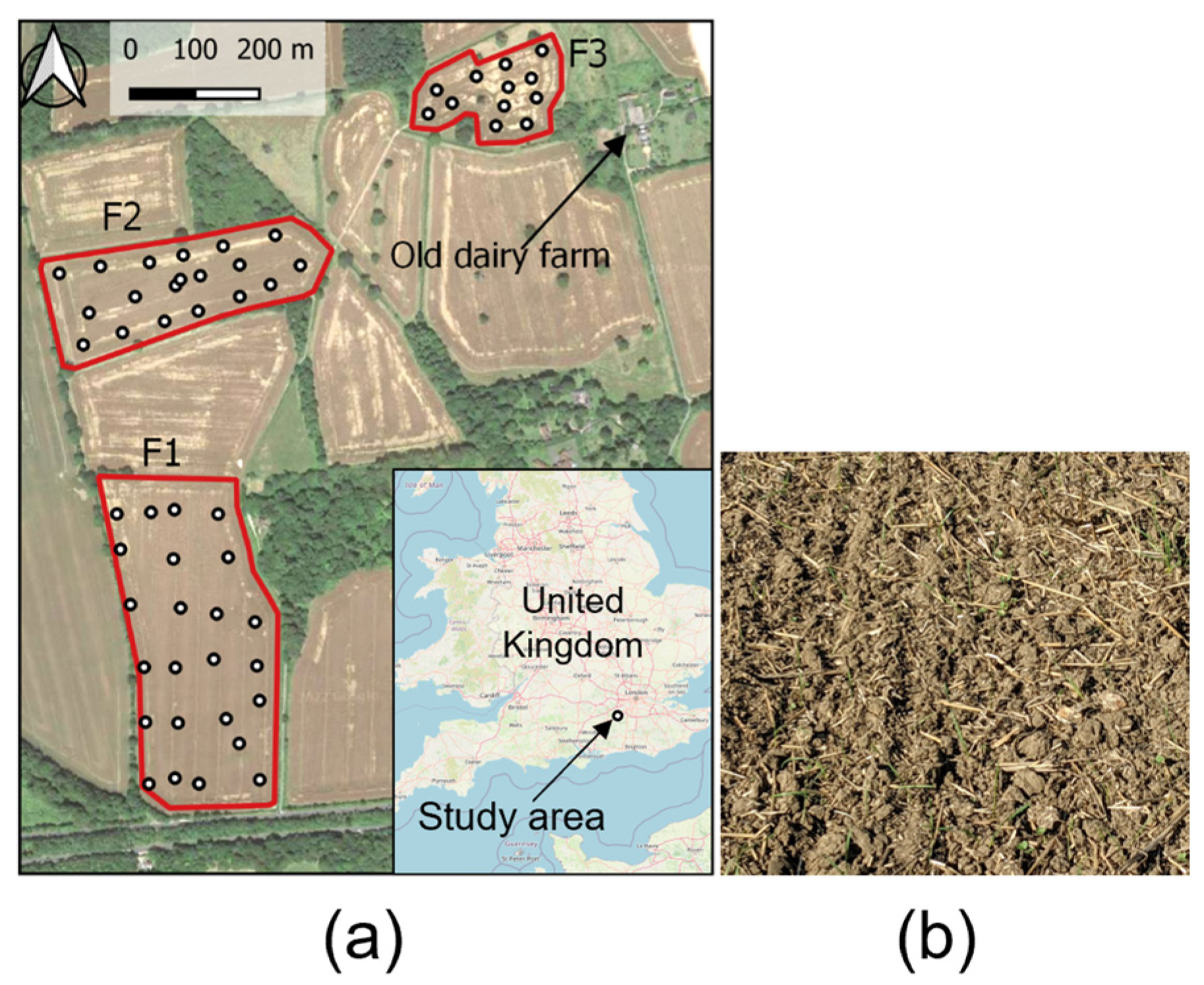
Figure 1. (a) location of the study fields: F1, F2, F3 (backgrounds from Google Earth and Open Street Maps), (b) close view of one of the sampling points.
Remotesensing 16 01510 g001
Figure 2. Map showing (a) SOC results and (b) elevation, shown in a graduated chromatic scale (Background image: Google Earth).
Remotesensing 16 01510 g002
Figure 3. Observed vs. predicted SOC model performance for RF (left panels) and SVR (right panels). Models use varied input data: SD, MD, T, SDT, and MDT. The coloured points indicate the data used for the 5-fold cross-validation whilst the black points correspond to the independent validation data.
Remotesensing 16 01510 g003
Figure 4. The permutation importance for the chosen Sentinel-2 bands and topographical features for SVR and RF.
Remotesensing 16 01510 g004
Figure 5. Models extrapolated to predict SOC over entire area of interest using SVR (a) and RF (b) for both MD (left) and MDT (right) (Background image: Google Earth).
Remotesensing 16 01510 g005
Table 1. Technical specification of Sentinel-2 bands used in this study [40].
BandSpectral Range (nm)Spectral Position (nm)Bandwidth (nm)Spatial Resolution (m)
B2458–5234906510
B3543–5785603510
B4650–6806653010
B5698–7137051520
B6733–7487401520
B7773–7937832020
B8785–90084211510
B8a855–8758652020
B111565–165516109020
B122100–2280219018020
Table 2. Spectral indices used in this study.
IndexDefinitionReference
Normalised Difference Vegetation Index (NDVI) ρ N I R     ρ R e d ρ N I R   +   ρ R e d Rouse et al. [44]
Normalised Burn Ratio (NBR2) ρ S W I R 1     ρ S W I R 2 ρ S W I R 1   +   ρ S W I R 2 Van Deventer et al. [43]
Enhanced Vegetation Index (EVI) 2.5 ρ N I R     ρ R e d ρ N I R   +   6 ρ R e d     7.5 ρ B l u e   +   0.5 Liu & Huete [46,47]
Green Normalised Difference Vegetation Index (GNDVI) ρ N I R     ρ G r e e n ρ N I R   +   ρ G r e e n Gitelson, Kaufman & Merzlyak [48]
Normalised Difference Red Edge (NDRE) ρ N I R     ρ R E 1 ρ N I R   +   ρ R E 1 Huete et al. [47]
Modified Triangular Vegetation Index 1 (MTVI) 1.2 1.2 ρ N I R     ρ G r e e n     2.5 ρ R e d     ρ G r e e n Haboudane et al. [49]
Normalised Difference Cloud Index (NDCI) ρ R E 3     ρ B l u e ρ R E 3   +   ρ B l u e Marshak et al. [50]
Optimised Soil-Adjusted Vegetation Index (OSAVI) ρ R E 2     ρ B l u e ρ R E 2   +   ρ B l u e Rondeaux, Steven & Baret [51]
Triangular Vegetation Index (TVI) 0.5 120 ρ R E 1     ρ G r e e n     200 ρ R e d     ρ G r e e n Broge & Leblanc [52]
Ratio Vegetation Index (RVI) ρ N I R ρ R e d Birth & McVey [53]
Chlorophyll Absorption Reflectance Index (CARI) ρ R E 1 ρ R e d 0.2 ρ R E 1     ρ R e d 200 ρ R E 1     ρ G r e e n Haboudane et al. [54]
Modified Soil-Adjusted Vegetation Index (MSAVI) 0.5 2 ρ N I R   +   1   +   2 ρ N I R   +   1 2     8 ρ N I R     ρ R e d Qi et al. [55]
New Vegetation Index (NVI) ρ R E 3     ρ R E 2 ρ R e d Gupta, Vijayan & Prasad [56]
Table 3. Hyperparameters for both models.
ModelHyperparameterDescriptionSearch Range
RFEstimator numberThe number of decision trees generated.500–25,000
Maximum DepthThe maximum depth a given tree can reach.5–4000
Feature proportionThe proportion of the total feature set used in decision tree construction.0.1–1.0
SVRRegularisation, CThe penalty associated with point distance.0.1–100
Epsilon, ε The distance from the hyperplane within which no penalty is applied. 0.001–100
Gamma, γ An RBF kernel coefficient determining the range of influence each point exerts.0.001–100
Table 4. Model name and input data.
Model NameInput Data
Single-date spectral (SD)Sentinel-2 spectral reflectance taken from one day only
Multidate spectral (MD)Median spectral reflectance of time series taken from Sentinel-2 over a 3 year period
Topographical (T)Topographical covariates (relative height, slope, TWI) extracted from high resolution DEM only
Single-date spectral and topographical (SDT)Both Sentinel-2 spectral reflectance data (target date only) and topographical covariates
Multidate spectral and topographical (MDT)Both median Sentinel-2 spectral reflectance data (3 year period) and topographical covariates
Table 5. SOC content statistics for each respective field.
FieldMinimum (%)Maximum (%)Mean (%)Standard
Deviation (%)
KurtosisSkewnessCoefficient of Variation (%)
F11.523.192.350.41−0.190.1617.65%
F21.632.522.060.25−0.780.1212.11%
F32.653.523.160.240.32−0.327.44%
Table 6. Performance of SOC prediction models for RF and SVR. The statistics include both the CV on the training set and the error from the validation set.
ModelAlgorithmMetricRMSE R 2 MAE
SDRFCross-validation 0.418 ± 0.047 0.413 ± 0.187 0.338 ± 0.082
Validation test 0.471 0.535 0.402
SVRCross-validation 0.301 ± 0.027 0.693 ± 0.066 0.228 ± 0.037
Validation test 0.531 0.408 0.449
MDRFCross-validation 0.354 ± 0.019 0.541 ± 0.141 0.292 ± 0.023
Validation test 0.346 0.696 0.269
SVRCross-validation 0.320 ± 0.028 0.633 ± 0.130 0.246 ± 0.042
Validation test 0.310 0.756 0.236
TRFCross-validation 0.462 ± 0.080 0.328 ± 0.344 0.339 ± 0.120
Validation test 0.515 0.445 0.433
SVRCross-validation 0.259 ± 0.028 0.762 ± 0.096 0.204 ± 0.040
Validation test 0.450 0.575 0.374
SDTRFCross-validation 0.332 ± 0.024 0.638 ± 0.030 0.267 ± 0.036
Validation test 0.395 0.672 0.292
SVRCross-validation 0.274 ± 0.019 0.739 ± 0.059 0.205 ± 0.032
Validation test 0.283 0.832 0.225
MDTRFCross-validation 0.337 ± 0.035 0.604 ± 0.084 0.273 ± 0.034
Validation test 0.293 0.782 0.243
SVRCross-validation 0.327 ± 0.044 0.525 ± 0.109 0.264 ± 0.062
Validation test 0.229 0.867 0.177
Disclaimer/Publisher’s Note: The statements, opinions and data contained in all publications are solely those of the individual author(s) and contributor(s) and not of MDPI and/or the editor(s). MDPI and/or the editor(s) disclaim responsibility for any injury to people or property resulting from any ideas, methods, instructions or products referred to in the content.