Article

Exploring Uncertainty-Based Self-Prompt for Test-Time Adaptation Semantic Segmentation in Remote Sensing Images

School of Geospatial Information, PLA Strategic Support Force Information Engineering University, Zhengzhou 450001, China
*
Author to whom correspondence should be addressed.
Remote Sens. 2024, 16(7), 1239; https://doi.org/10.3390/rs16071239
Submission received: 23 January 2024 / Revised: 20 March 2024 / Accepted: 28 March 2024 / Published: 31 March 2024

Abstract

:
Test-time adaptation (TTA) has been proven to effectively improve the adaptability of deep learning semantic segmentation models facing continuous changeable scenes. However, most of the existing TTA algorithms lack an explicit exploration of domain gaps, especially those based on visual domain prompts. To address these issues, this paper proposes a self-prompt strategy based on uncertainty, guiding the model to continuously focus on regions with high uncertainty (i.e., regions with a larger domain gap). Specifically, we still use the Mean-Teacher architecture with the predicted entropy from the teacher network serving as the input to the prompt module. The prompt module processes uncertain maps and guides the student network to focus on regions with higher entropy, enabling continuous adaptation to new scenes. This is a self-prompting strategy that requires no prior knowledge and is tested on widely used benchmarks. In terms of the average performance, our method outperformed the baseline algorithm in TTA and continual TTA settings of Cityscapes-to-ACDC by 3.3% and 3.9%, respectively. Our method also outperformed the baseline algorithm by 4.1% and 3.1% on the more difficult Cityscapes-to-(Foggy and Rainy) Cityscapes setting, which also surpasses six other current TTA methods.

1. Introduction

In the actual operation of intelligent vehicles, it is necessary to establish a high-level understanding of the environment to assist decision making [1,2]. There is a need to build the real-time and accurate perception capability through effective data management and processing methods [3,4]. Among various perception methods, machine vision-based methods have become an important part due to their comprehensive, intuitive, and cost-effective advantages [5]. Semantic segmentation [6], in particular, can directly determine the positions and occupancy of various entities in the scene, thereby effectively aiding intelligent vehicles. Real-world scenes are often complex and diverse, varying in city styles and weather (such as rain, fog, snow, and nighttime) [7,8,9]. However, segmentation models trained offline and based on a fully supervised paradigm often lack generalization in these unseen or adverse conditions. Therefore, a lot of works adopted Domain Adaptation (DA) [10,11,12,13,14,15,16,17,18] to train, attempting to transfer the knowledge from existing datasets to unlabeled environments. Although DA effectively improves the model’s generalization, it still follows an offline training approach, which fixes the model’s performance in real-world scenarios once training is complete, making it difficult to adapt to other more complex scenes. Considering that some acronyms will be used frequently, we have listed the acronyms at the end for facilitating reading and understanding the paper.
Another direction is to explore the commonalities between data with different distributions, which is called Domain Generalization (DG, or OpenDA) [19,20,21,22,23,24,25]. This strategy aims to extract domain-invariant knowledge from a wide range of data, hoping to achieve better performance on unseen target domains. In addition to using real data, synthetic datasets [24,25] are also widely used in DG. Various training augmentation [20,21] and test augmentation methods [22,23] also fall into this category. Although DG attempts to address the generalization problem from a more macro-perspective, the common features extracted by DG are often weak to capture the variations in real-world scenes.
Test-time adaptation (TTA) [26,27,28,29,30,31] aims to make models adapt different conditions during testing. TTA can deal with newly arriving data, thereby updating the knowledge stored in the model. According to the trend of changes in the test data, TTA can be divided into continuous TTA [32] and non-continuous TTA. Continuous TTA is specifically designed to handle scenarios with continuous changes, making it particularly suitable for automated vehicle perception. However, continuous TTA faces two challenges: (1) how to effectively extract knowledge from unlabeled data, and (2) how to avoid or mitigate catastrophic forgetting. This is because the model can be easily affected by wrong predictions and noise during long-time adaptation.
Previous TTA approaches can be categorized into distribution alignment strategies [28,29,30,31] and consistency learning strategies [27,32]. Distribution alignment strategies assume that the distribution differences between two domains can be characterized by the parameters of normalization layers. Therefore, continuous domain discrepancy alignment can be achieved by adjusting normalization layers such as Batch Normalization (BN) [33]. However, it should be noted that not every neural network has BN layers, and fine-tuning BN layers usually cannot accurately capture domain differences in most cases. On the other hand, consistency learning employs semi-supervised learning by using a Mean-Teacher architecture [34] to generate pseudo-labels for multiple augmented images based on the teacher model and calculate the consistency loss between the student model and the teacher model. Here, the motivation for this adaptation method is not clear, and the introduction of test-time augmentation [22] significantly slows down the training speed. To address catastrophic forgetting [35], stochastic parameter restore [32] and regularization [27] are commonly used. Random parameter recovery periodically reassigns a portion of the original model’s parameters to the current model to counteract forgetting, while regularization attempts to constrain the model to make it less sensitive to domain changes. Although these two methods effectively alleviate forgetting, they also conservatively limit the model.
With the rise of large-scale models [36,37,38], the use of prompt tuning [36] techniques in Natural Language Processing (NLP) has been introduced to computer vision as a highly promising direction. Prompt allows for the preservation of the original model while using additional learnable parameters to handle the features of newly encountered data [39]. Recently, some studies have proposed the concept of Visual Domain Prompt to address domain gaps [40,41,42], but they often focus on classification tasks. There is also the problem that domain prompts lack clear meaning (as is shown in Figure 1). It is worth noting that the prompt holds great potential for building domain cues for models, which will help acquire knowledge from unlabeled data, and persistent prompts with additional learnable parameters are expected to alleviate the forgetting.
We believe that the domain gap is the fundamental reason for increased uncertainty in model predictions. The role of the prompt should be to guide the model’s attention to areas of high uncertainty, thereby helping the model achieve stability during testing. To address this problem, we propose a Uncertainty-based Self-Prompting (USP) method to assist the model to adapt during testing. The method still utilizes the Mean-Teacher architecture, where the teacher model not only generates pseudo-labels but also produces uncertainty maps. Then, the testing images, uncertainty maps and the prompt module are collectively used as visual prompts for the student model’s computation. This method effectively guides the model to focus on regions with high uncertainty (i.e., areas with significant domain differences) and helps the model explore cross-domain information. Regarding alleviating forgetting, we do not follow VPT [39] (this method freezes the backbone and only trains the prompt and segmentation heads) and adjust all the parameters. Additionally, after each adaptation, the prompt module updates the next prediction’s prompt using the exponential moving average (EMA) technique. We compared our algorithm with six other online TTA algorithms, one continuous TTA algorithm [32] as well as five applied on intelligent vehicle segmentation methods. Specifically, we conduct experiments on three benchmarks (Cityscapes [43], Foggy and Rainy-Cityscapes [7], and ACDC [9]) and demonstrate its superiority in terms of accuracy and efficiency. The structure of the paper is as follows. In Section 3, we describe the detail of our method, including an uncertainty prompt and domain prompt update strategy, etc. In Section 4, we set TTA and CTTA experiments to compare the performance of our method with other state-of-the-art methods; then, the ablation studies and discussion are conducted in Section 5.
Our contributions can be summarized as follows:
  • We propose a self-prompted test-time adaptation method based on uncertainty, which does not require any prior knowledge, and effectively directs the model’s attention to domain gap adaptation. At the same time, our method effectively improves the anti-forgetting ability and maintains effective performance over multiple rounds of continuous adaptation.
  • Our proposed method surpasses six previous online TTA methods and one continuous TTA semantic segmentation method, demonstrating its effectiveness in cross-domain learning.

2. Related Work

2.1. Road Scene Semantic Segmentation

There have been numerous studies on understanding road scenes using deep learning methods. A survey [6] highlights the importance of semantic segmentation in autonomous driving scene understanding. DSiV [4] and [44] integrate visual data into the field of autonomous driving data science. Building upon these works, [45] proposes a hierarchical and interpretable approach to autonomous driving, providing a multi-scale perspective for future research. FCIS [46] introduces an instance-level pixel inference method for more accurate contour detection, while [47] presents a scene-adaptive multi-scale semantic perception framework for 3D semantic segmentation, estimating spatial occupancy in the scene. MPCNet [48] proposed a multi-pool contextual segmentation network with high speed. FT-Net [49] tries to use few-shot learning to improve segmentation results. However, these methods do not consider the segmentation performance under adverse imaging conditions and need to improve adaptability to scene variations.

2.2. Domain Adaptation

Domain adaptation aims to transfer knowledge from one (source) domain to another (target domain). Typically, labels in the source domain are easily obtained, such as synthetic data (e.g., GTA5 [50] and SYNTHIA [51]) and annotated real data (e.g., Cityscapes [43]), while labels in the target domain are difficult to acquire. This leads to a poor generalization of models trained on the source domain datasets [52]. Early domain adaptation methods primarily used generative adversarial networks [53], treating the domain gap as perturbations or noise, trying to align the two domains through regularization [11,12,54]. However, this approach was too coarse in computing discriminative probabilities. Subsequently, many works attempted contrastive learning for domain adaptation, using the source domain as a reference to guide model learning in the target domain. DISE [55] separates image features into domain-invariant and domain-specific features. ProDA [56] utilizes prototypes for learning. DAFormer [10] is the first to introduce the Transformer [57] into domain adaptation tasks and adaptively adjusts the target domain loss weights during training to guide capability transfer. HRDA [17], built upon DAFormer, integrates high-resolution attention prediction. MIC [18] introduces masked learning [58], aiming to let the student model recover the masked spatial structure and enhance spatial consistency in domain adaptation. ALST [59] summarizes the domain adaptive segmentation algorithms applied to intelligent vehicles. However, domain adaptation still relies on offline learning and struggles with the contradiction between unlimited test data and limited training data.

2.3. Test-Time Adaptation

Test-time adaptation (TTA) aims to make models adapt to newly coming data during testing. Theoretically, TTA enables infinite testing data be used for training, achieving lifelong learning [60]. During TTA, no source domain data are needed, forcing the TTA algorithm to self-supervised train entirely in the target domain. The initial challenge for TTA is how to acquire knowledge from unlabeled test data. Some approaches use generative models for feature alignment [61], while others utilize regularization methods to fine-tune existing models [28,29]. For instance, TENT [28] adjusts the BN layer through entropy minimization. Another problem in TTA is overcoming the forgetting [35] caused by continuous training. Some approaches employ periodic replay-based correction [62], while most methods adopt regularization techniques [27,30,31] aiming to constrain the model’s attention to domain-invariant robust features, reducing interference from erroneous details. CoTTA [32] tackles the scenario of continuous domain changes by developing a domain adaptation architecture suitable for any model. It mitigates forgetting by utilizing random parameter restoration and improves performance on the testing set through test-time augmentation and weight-averaged teacher knowledge collection. Nonetheless, these methods lack an explicit handling of domain discrepancy in their motivations, resulting in weakness when address the difficult challenges posed by domain gaps.

2.4. Visual Domain Prompt

Prompt originated from large-scale natural language processing models [36] and has been introduced to the computer vision domain. In NLP, prompts are commonly presented as questions or fill-in-the-blank forms, aiming to guide the model to recover the missing parts. Therefore, early applications of prompts in computer vision with large models were primarily task prompts [38,63], attempting to guide the models to complete the desired tasks through task examples. Subsequently, some works attempted to tune the models using prompts. VPT [39] introduced learnable parameters into prompts and achieved good optimization results with freezing the backbone network. Later, DePT [41] incorporated the idea of VPT into TTA by adding prompts to the memory pool for feature aggregation. VDP [40] first proposed the concept of Visual Domain Prompt, which froze the model’s backbone, utilized learnable parameters to randomly mask the model, and set domain-specific and domain-agnostic prompts. However, this kind of prompt still lacks interpretable domain specificity. SVDP [64] employed uncertainty maps generated by MC-Dropout to guide the model to focus on areas with significant domain discrepancies sparsely. SVDP [64] enables prompts to possess domain-aware properties for the first time. In this paper, we use entropy to represent uncertainty, with the predicted image, entropy map and learnable parameters as components of the Visual Domain Prompt, enhancing the model’s ability to fuse global domain discrepancy features.

3. Method

3.1. Preliminaries

3.1.1. Test-Time Adaptation (TTA)

TTA aims to utilize a pretrained model on the source domain ( X S , Y S ) to adapt to unlabeled and potentially differently distributed, X T 1 , X T 2 X T n during testing, where X T i = x i T i = 1 N t , N t represent the scale of the target domain. The overall training only has access to target domain data once and cannot access the source domain. The target domain for TTA can be a single one or multiple continually changing unknown domains (CTTA) with the latter more in line with that of the real world.

3.1.2. Visual Domain Prompt

VDP [40] first introduced Visual Domain Prompt to serve the continual adaptation of classification tasks. Specifically, VDP( p ) is a dense set of learnable parameters added to the input image:
x ˜ = x + p

3.2. Overview

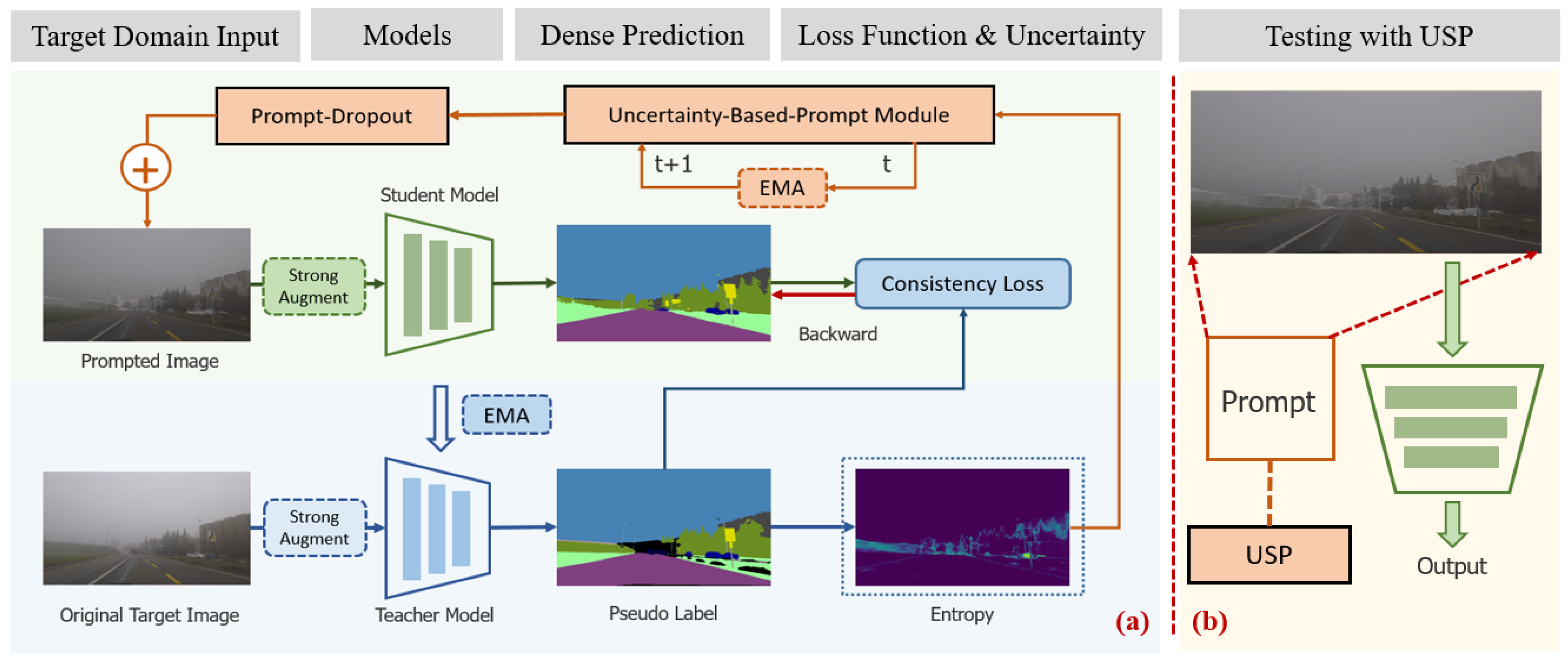
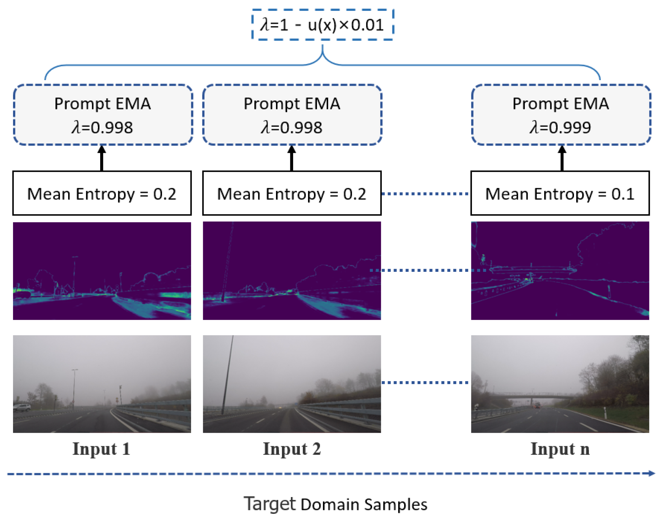
We try to let the model handle the domain gap according to uncertainty by itself. The overall framework is shown in Figure 2, which still adopts the Mean-Teacher [34] architecture, in which a robust weighted-averaged teacher model f θ T generates prompts by the uncertainty, thus guiding the student model (main model) f θ S to reinforce learning in regions with significant domain differences. Our approach is a compromise between the Dense Rectangular Prompt (VDP) [40] and the Sparse Prompt (SVDP) [64]. To mitigate the overconfidence of the model (where high uncertainty does not necessarily mean wrong predictions), prompts are randomly dropped, referred to as Prompt Dropout. After each testing adaptation, the parameters of the current prompt are transferred next time using an Exponential Moving Average (EMA) [65], which is shown in Figure 3. Following previous work [32,64], the loss function still employs consistency loss between the student output and pseudo-labels generated by the teacher model. Concretely, the original target images will undergo strong augmentation to obtain a pseudo-label, and the entropy of teacher’s prediction will be the original hint. Next, the uncertainty-based prompt module will process the prompt features, which are then randomly dropped. Finally, the prompt will be added on the original image. During the test-time adaptation, the prompt module will be updated by a historical version of the last iteration. After being prompted, the student model will pay more attention to high-entropy regions and attempts to restore the original image features compared to the pseudo-label, achieving similar effects to Masked Image Learning.

3.3. Uncertainty Prompted and Dropout

For single test data x t , we adopt Shannon entropy [66] H ( y ^ ) of the teacher prediction H ( y ^ ) = c f θ T ( y ^ ) log f θ T ( y ^ ) as a measure of uncertainty. During the adaptation process, the weighted-averaged teacher model f θ t accumulates knowledge, allowing its entropy distribution to express the model’s adaptability to the current target domain. In sparse (or image-level) tasks such as classification, optimizing the loss function with respect to entropy may result in the model assigning probability to all classes [28]. However, in dense (or pixel-level) tasks like semantic segmentation, the distribution of entropy possesses clear spatial properties. Furthermore, our method treats entropy merely as a prompt without considering its specific semantic information, thereby facilitating the model to conduct more targeted optimization.
After obtaining the entropy map H ( y ^ ) , we employ a prompt module E consisting of convolutional layers to jointly process with the image x t . Specifically, we concatenate the entropy map as the fourth channel of x t and then encode the image and the entropy map to the prompt feature f :
f = E ( [ x t , H ( y ^ ) ] )
Although the entropy indicates where the model should pay more attention, high entropy cannot confirm the model’s predictions here are incorrect. To avoid over-fitting, we employ random dropout, which proposed stochastic abandon uncertain features in f . Specifically, we generate a mask M using the Bernoulli distribution with probability p and randomly drop out features from f that exceed a certain threshold τ .
M Bernoulli p
p r , c = f r , c M r , c = 1 f r , c < τ 0 M r , c = 0 f r , c > τ
where the r and c are the row and column number of H ( y ^ ) , respectively. The processed prompts are added to the image, constituting the final image which will be fed into the main model. Thus, the domain information will be encoded:
x ˜ T = x T + p

3.4. Domain Prompt Updating

We follow prior works [10,34,64] to perform exponential moving average (EMA) [65] parameter updates between teacher–student networks and the prompt module, which is shown in Figure 3. We believe that the knowledge in the prompt module should be temporally updated, and the degree depends on the current mean entropy value. If it is small, the prompt should be relatively stable, and more weights from previous iterations should be reserved. The parameters θ T t of teacher model are updated by θ S t of the student model by Equation (6):
θ T t + 1 = α θ T t + ( 1 α ) θ S t
For the prompt module E, we hope it can accumulate temporal information and not be limited to encode the domain information of the current image; thus, more domain-invariant features can be encoded as well as the relationship underlying the uncertainty map H ( y ^ ) and the original image x T . Therefore, we follow SVDP [64] to update the prompt module based on the image-level uncertainty. We assume that if the uncertainty π ( x T ) is low, there is a higher probability of accurate predictions, and thus minimal modifications are needed for the prompt module and vice versa. Here, we use Equation (8) to define the EMA hyper-parameter in Equation (7), which is also shown in Figure 3.
E t = λ E t 1 + ( 1 λ ) E t
λ = 1 ( π ( x T ) ) × 0.01

3.5. Loss Function

Like previous TTA methods [32,64], we utilize the teacher model f θ T to generate pseudo-labels y ^ T which are then refined through test-time augmentation [23] and confidence filtering. Subsequently, we employ the pixel-wise cross-entropy consistency loss as the objective function for optimization.
L c o n ( x ˜ T ) = w , h W , H c = 1 C y ^ T ( w , h , c ) log y ˜ T ( w , h , c )
where C means the number of categories and y ˜ T is the output of the student model f θ S . When applying test-time augmentation, this function will execute multiple times to complete the consistency training between the original image and several augmented images.

4. Results

4.1. Task Settings

4.1.1. TTA and CTTA

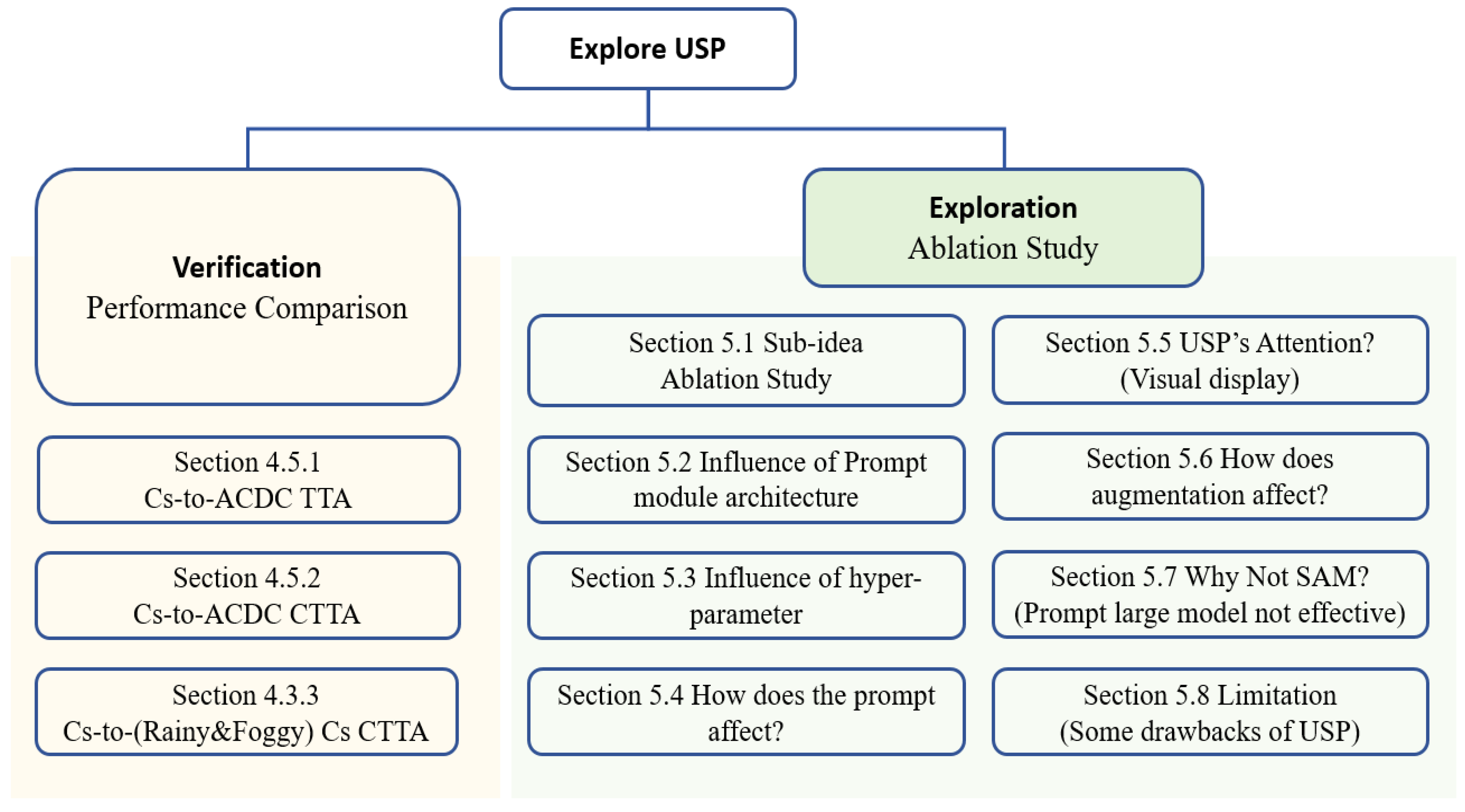
Both tasks aim to make the pretrained model on the source domain adapt the unseen target domains. During adaptation, the source domain is inaccessible, and the data from the target domain can only be accessed once. The basic setting of continual test-time adaptation (CTTA) is similar to TTA, but it involves a continuously changing target domain sequence, which introduces additional challenges. For facilitating reading, the design of all the experiments is shown in Figure 4.

4.1.2. Cityscapes-to-ACDC

In all the TTA scenarios, we use Cityscapes [43] as the source domain to pretrain the model. ACDC [9] is a semantic segmentation benchmark specifically designed for cross-domain learning tasks. It comprises four challenging conditions: fog, rain, snow, and night. For the TTA task, our approach will make each pretrained model individually adapt to each scene. In case of CTTA, we follow previous work [32,64] and simulate real-world variations by repeating the same sequence of target domains (Fog→Night→Rain→Snow) multiple times. As the ACDC dataset is constructed by extracting video frames, it inherently possesses the attribute of temporal continuity.

4.1.3. Citsycapes-to-(Foggy and Rainy) Citsycapes

These two datasets [7] apply synthetic fog and rain to Cityscapes [43] images. Compared to ACDC [9], Foggy and Rainy Cityscapes are more difficult due to the larger density of adverse condition factors. Following the previously mentioned TTA configuration, we adapt the model to each scene individually.

4.2. Dataset and Metrics

The datasets are listed in Table 1. Cityscapes is only used to train the source domain model and does not participate in the adaptation process. The remaining datasets serve as benchmarks for evaluating the performance. TTA tasks differ from other tasks in that all images in its training set will be passed in once as “test data”, so the model needs to be evaluated on its training set images. The Foggy and Rainy Cityscapes dataset contained images with various levels of synthetic adverse conditions, and only the lightest 2975 training images were selected for evaluation. The ACDC dataset is divided into subsets of four weather types, each of which includes about 400 and 100 labeled images in the training and validation set, respectively. We use the mIoU (mean Intersection over Union) and mAcc (mean accuracy) as the evaluation metrics. Assuming there are a total of k + 1 classes, in which 1 is the background class, and p i j represents the number of pixels labeled as class i and predicted as class j; then, mIoU and mAcc can be calculated as follows:
mIoU = 1 k + 1 i = 0 k p i i j = 0 k p i j + j = 0 k p j i p i i
mAcc = 1 k + 1 i = 0 k p i i j = 0 k p i j

4.3. Experiment Workflow

In Figure 4, we show the idea of the whole experiment. In order to explore the USP proposed in this paper, we divided the experiment into two parts. The first part includes the Verification experiment, which compares the performance of our USP with other methods, including the performance comparison results under three experimental settings. This section corresponds to Table 2, Table 3, Table 4 and Table 5 and Figure 5. The second part includes the Exploration experiment, which mainly explores the function of each subcomponent (Table 6), and the influence of hyper-parameters (Figure 6 and Figure 7) and prompt module structure on the performance (Table 7). We then highlight the visualizations of the prompt module (Figure 8 and Figure 9), show the influence of augmentation (Table 8 and Figure 10) and explain the reasons for not using the existing large-scale segmentation model (Figure 11 and Table 9). Finally, we show some drawbacks of our methods (Figure 12) and analyze the possible reasons. All acronyms are shown in Nomenclature section.

4.4. Implementation Details

We followed the basic implementation details in [32,64] to set up our semantic segmentation TTA experiment based on a segmentation framework [71]. Specifically, we used the SegFormer-B5 [57] model pretrained on Cityscapes [43] as our source model. In terms of data, we down-sampled the 1920 × 1080 images to 960 × 540 as input. We also used the Adam optimizer [72] with ( β 1 , β 2 ) = (0.9, 0.999), set the learning rate to 3 × 10 4 and set the batch size to 1. During the TTA process, we employed the same test-time augmentation strategy as SVDP [64]. The prompt module is designed with an Encoder–Decoder architecture consisting of eight convolutional layers (will be explained in detail in Section 5.2), producing neural prompt points with three channels as output. We set the hyper-parameters: EMA update coefficient α = 0.99 (in Equation (6)), randomly dropout probability p = 0.5 (in Equation (3)) and high entropy threshold τ = 0.85 (in Equation (4)). The ablation study will be shown in Section 5.3. All experiments were conducted on NVIDIA Tesla V100 GPUs.

4.5. Performance Comparison

4.5.1. Cityscapes-to-ACDC TTA

We evaluate our TTA method on the four individual adverse-condition subdatasets of ACDC [9], as shown in Table 2. The original ERFNet [67], IAL [68], MLFNet [69], EIE [70] and SegFormer [57] were only trained on the source domain and exhibited its inherent generalization across the four scenarios. The above algorithms, which are already suitable for intelligent vehicles, show a performance decline in each of these adverse scenarios. TENT [28] employed a relatively simple domain alignment approach, leading to some degree of under-fitting. CoTTA [32] achieved performance improvement due to the strongly augmented contrast learning during testing. Compared with CoTTA, our method achieved a 2.3% and 1.9% increase in mIoU and mAcc under Fog weather, indicating our method’s stronger ability to handle the domain gap. In night, rain, and snow conditions, our method also outperformed CoTTA by 3.7%, 3.8% and 3.4%, respectively. Although SDVP [64] is a formidable competitor in this study, it had a slight deficiency in the night scene due to the entropy distribution not being as accurate as in the day scene, especially sky and vegetable categories.

4.5.2. Citsycapes-to-(Foggy and Rainy) Citsycapes TTA

We also evaluate our method on more challenging Foggy and Rainy Cityscapes [7], as shown in Table 5. We no longer compare ERFNet [67] and similar algorithms; only the strongest SegFormer is represented. We observe a similar trend to Cityscapes-to-ACDC TTA. Our approach significantly outperforms the baseline method CoTTA by 4.1% and 3.1% in Foggy and Rainy scenes, respectively, demonstrating its ability to generalize well in rainy and snowy scenes.

4.5.3. Cityscapes-to-ACDC CTTA

Finally, we repeate the four adverse-condition scenarios of ACDC multiple times to simulate continuous change and evaluate the forgetting resistance, as shown in Table 3. In the three rounds, “Source” freezes the original ERFNet [67], IAL [68], MLFNet [69], EIE [70] and SegFormer [57] pretrained weight, so the performance remained consistent. TENT [28] and DePT [41] showed noticeable degradation because their parameters were continuously influenced and perturbed by the new data. It is worth noting that the structure of DePT [41] is not very suitable for the dense prediction task of TTA because the memory pool cannot meet the requirements. With the benefit of stochastic parameter restoration, CoTTA [32] maintained stable performance without obvious degradation. VDP [40], which completely froze the original model and only modified the prompt, also maintained good performance. However, it was not specifically designed for dense prediction tasks, so its performance was not as good as CoTTA. SVDP [64] has good performance by sparse prompts, but it also experienced obvious degradation (such as “fog”, mIoU from 72.5 to 72.0). On one hand, our method improved by 5.6% over the CoTTA baseline during the three adaptation rounds. On the other hand, our method has surpassed SVDP comprehensively (including night scenes) from the third adaptation round, demonstrating its good adaptability and stability.

5. Discussion

5.1. Effectiveness of Each Component

In Table 6, we design six experiments to explore the contributions of each component. They are conducted in the Cityscapes-to-ACDC (fog) TTA scenario. TS, USP, DPU, and P-Drop represent the adoption of teacher–student architecture [34], uncertainty-based prompt, domain prompt updating, and prompt dropout, respectively. E x 1 does not employ any TTA strategy, meaning it uses the pretrained model of SegFormer. E x 2 utilizes the teacher–student mode, which refers to weight-averaged teacher [34]. E x 3 adds the uncertainty-based prompt on top of E x 2 , and E x 4 includes domain prompt updating. E x 5 randomly applies dropout to USP. E x 6 represents the complete configuration. It can be seen that after the adoption of USP, the model’s performance improves the most, reaching up to 3.0%, compared to using only TS. Furthermore, the model’s performance increases by 0.5% and 0.1% when DPU and P-Drop are employed. This indicates that USP, as the core innovation, effectively utilizes uncertainty to guide the model toward better generalization. Since the ACDC [9] dataset exhibits a relatively uniform distribution with smooth change, the uncertainty within the same subset fluctuates within a certain range. Therefore, the knowledge provided by the previous prompt module has limited impact. After all configurations are added, no interference between modules happened, resulting in optimal performance.

5.2. How Does Prompt Architecture Affect the Performance?

We have explored the effect of prompt’s architecture. The experiments were conducted on the Cityscapes-to-ACDC (fog) TTA dataset. We have also observed similar phenomena in other scenes. The prompt module mainly includes convolutional layers and is divided into four architectures: small, medium, large, and huge, based on the number of parameters. The meanings in Table 7 represent the size of the convolutional kernel and the number of output channels. The prompt module will process the entropy map and target image to output three-channel images that can be compatible to input. As shown in Table 7, the best results are achieved by Prompt_M, which only contains 0.04 M parameters, indicating that prompt generation can be accomplished using parameters by adding 1–2%. The table also demonstrates that more parameters do not necessarily lead to better performance. Excessive parameters may result in over-fitting to the image information. Additionally, due to the weak gradient propagation, it is not advisable to use a deep architecture for the prompt module.

5.3. How Do the Hyper-Parameters Affect the Performance

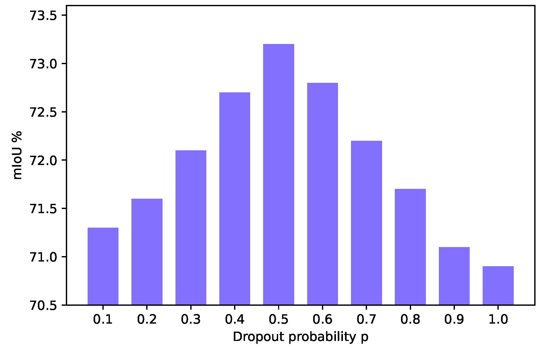
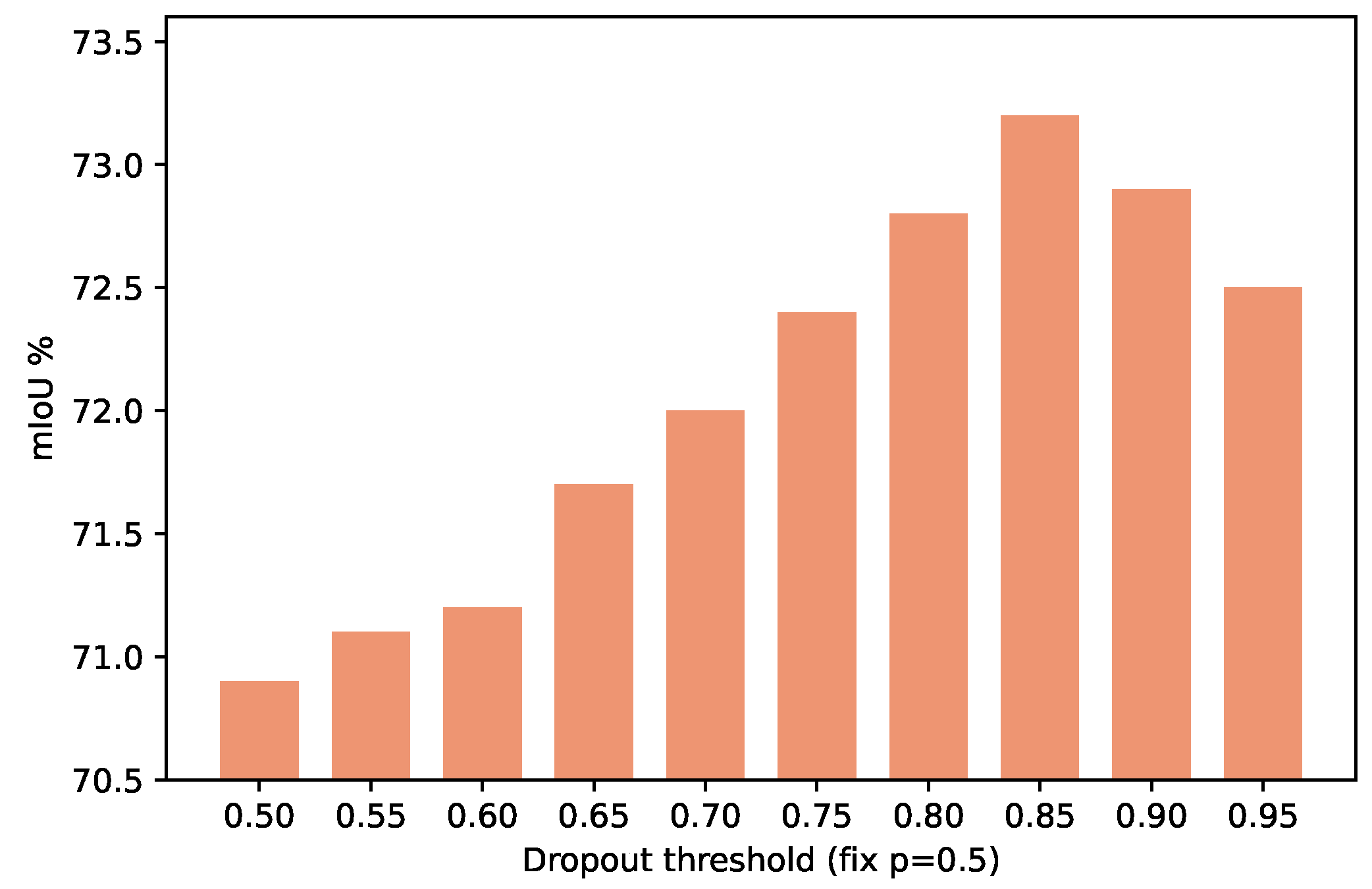
In our USP framework, there are two hyper-parameters, which are included in Equations (3) and (4): the probability p for randomly dropout prompts and the probability τ for retaining prompt features. Both these parameters have a certain peak-like property, meaning that being set too small will affect the regularization, while be set too large can render the prompt module almost ineffective. We conducted experiments on the Cityscapes-to-ACDC (night) dataset, as shown in Figure 6 and Figure 7, to explore the effects of these two hyper-parameters. For p, the range is ( 0 , 1 ) . For τ , we considered ( 0.5 , 1 ) as a reasonable range based on statistical analysis of tensor values. Firstly, we fix τ at 0.75 and test different p values. We found that p = 0.5 yielded the best results. Similarly, by fixing p = 0.5 and testing different τ values, we found that τ = 0.85 yielded the best results. When p 0 or p 1 , the performance of the model tends to degrade toward the baseline CoTTA [32].

5.4. The Visual Effect of Prompt

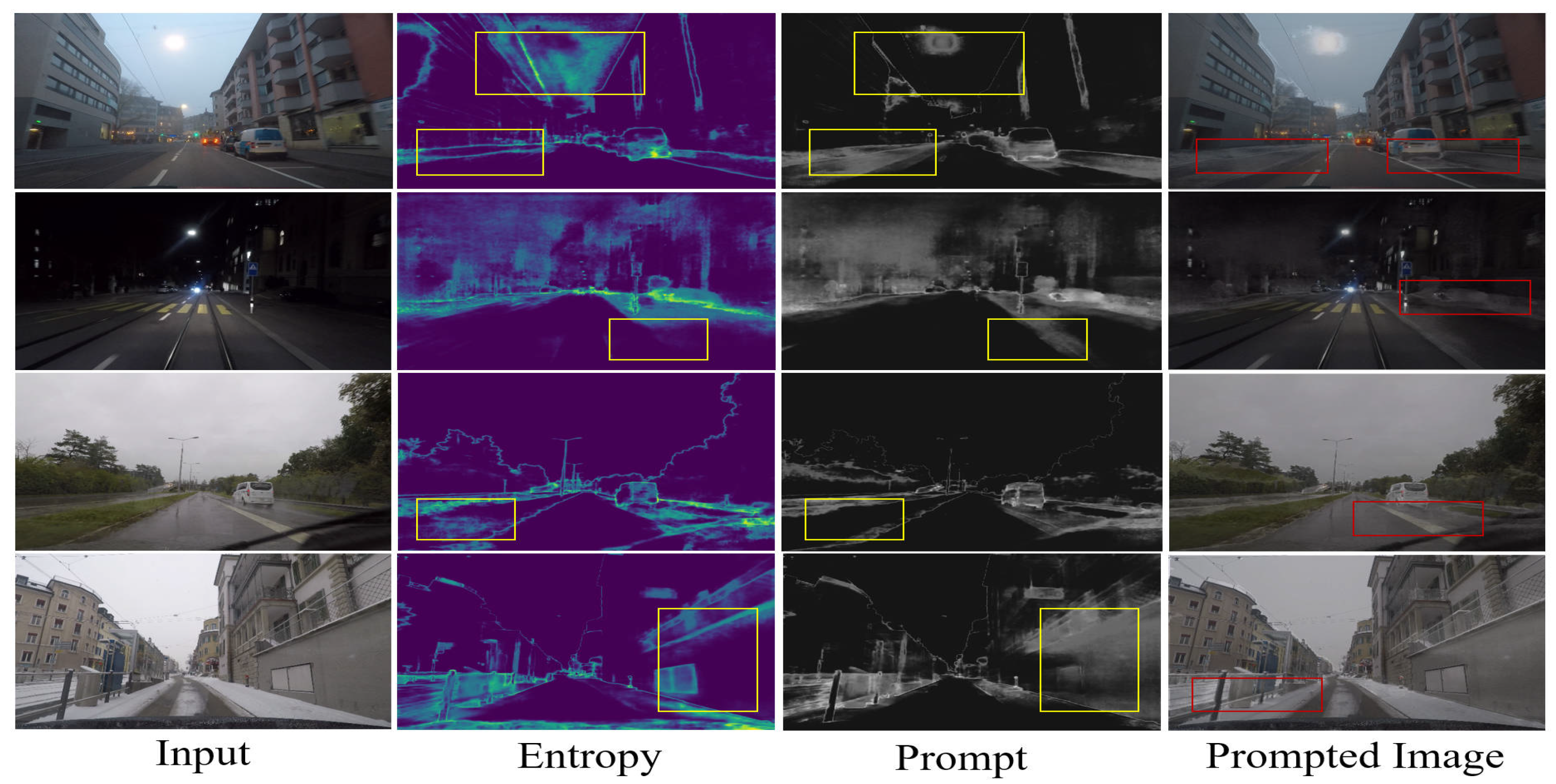
In Figure 8, we illustrate the visual effect of the prompt. Since the prompt module outputs a three-channel image that is difficult to distinguish after merging with the original image, we applied some enhancement methods for visual representation. Here, the visual domain prompt mostly preserves the distribution of entropy, placing some cues in regions with higher uncertainty. However, the prompt module also produced some different interpretations, such as the parts framed by the yellow boxes in the Figure 8. We believe that these different outputs are the combined integration of entropy and image information, which will help to produce more comprehensive judgement. For example, in the foggy scene (1st row in Figure 8), the entropy is higher in the sky area, but the prompt module considers it more important to focus on the ground after learning. Similarly, in the rainy image of the second row, the entropy is high in the lawn area, but the prompt module deems it unnecessary to pay much attention there, whereas in the snowy image of the fourth row, the prompt module considers the nearby wall surface to be more critical. Thus, the added prompt tries to introduce regularization to specific areas (with a larger domain gap). In SVDP [64], this regularization is more sparse, resulting in there not being enough cues. In VDP [40], the cues are too dense with their placement, and their meaning is unclear. Our proposed USP applies a continuous and dense prompt, allowing the model to make smoother predictions with considering contextual information. On the other hand, the role of the prompt is somewhat similar to masked image modeling [58]. The teacher receives the complete target image as input; hence, the generated pseudo-labels can be considered complete. By adding the prompt, the image is perturbed (like being masked), and then the student network needs to learn how to “restore” the original information, thereby enhancing robustness.

5.5. Attention and Specific Performance Affected by USP

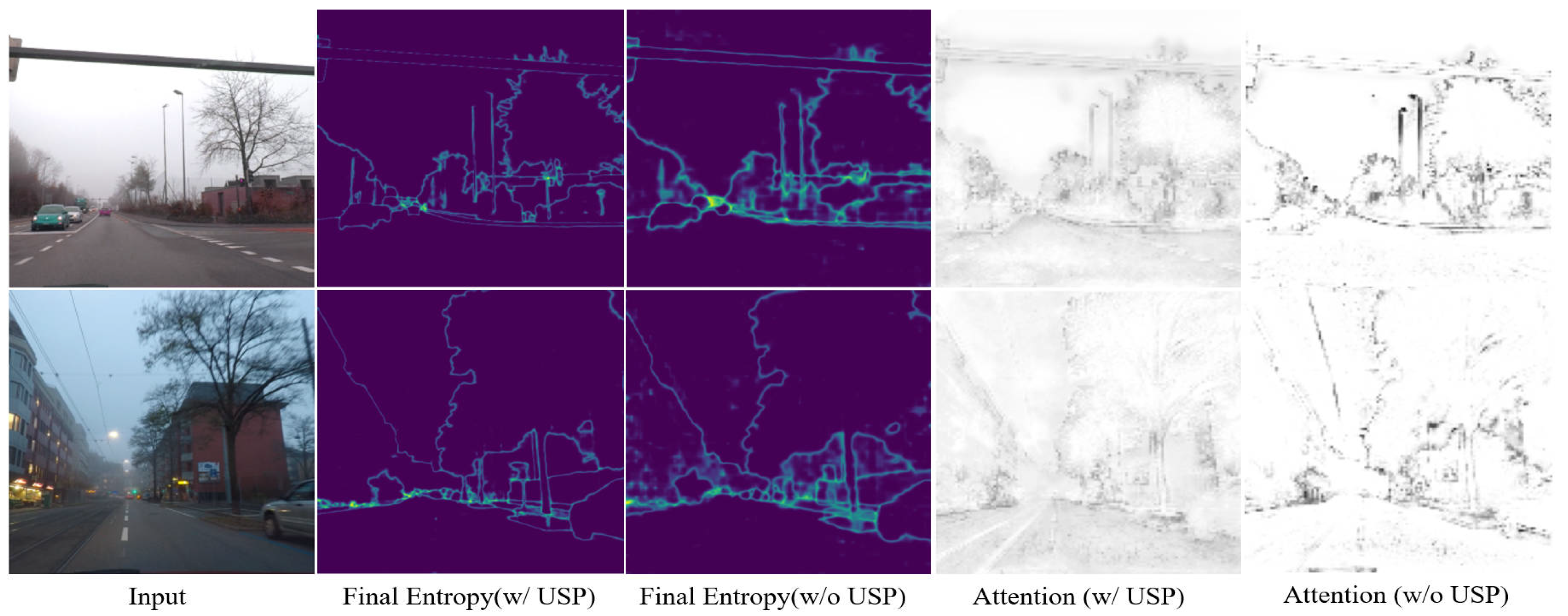
To further explore the impact of entropy self-prompting, we added a decoding head to the segmentor for collecting attention information. As is shown in Figure 9, we test two models (one that had undergone USP and one without USP) and display their predicted entropy with attention values. The higher the attention value, the deeper the color. We can see that the model without USP training outputs higher prediction entropy and experiences more dramatic attention changes, reflecting the model’s sensitivity to textures, shapes, and other information (which are easily affected by the domain gap) in the image. On the other hand, the model has lower entropy with the attention being more evenly distributed after the USP training, indicating the model has good adaptability to various parts, thereby suggesting better generalization.
In Table 4, we present the recognition performance of models trained with and without USP across four different scenarios for each category. Corresponding to the TTA section in Table 2, w/o USP refers to the baseline method COTTA [32]. We found that in foggy conditions, the “road” and “train” categories achieved accuracy rates of 93.5% and 88.9%, respectively, which are 10.5% and 8.2% higher than the baseline COTTA on the “Bike” and “Fence” categories. In the night scene, the improvement was slightly less, with the “Building”, “Terrain”, and “Truck” categories reaching 79.2%, 41.2%, and 26.4%, respectively. Some declines appears, indicating that nighttime poses significant interference, which is also reflected in other TTA methods. In the rainy condition, our method effectively overcomes the presence of water on the ground, achieving recognition rates of 88.2% for the “road” category, 90.4% for the “building” category, and 60.3% for the “wall” category, which confirms the effectiveness in adjusting the model’s attention. In the snowy condition, our method also achieved improvements in some difficult categories (such as “train” and “bus”). Therefore, our approach is adaptable to challenging categories in the test scenarios.

5.6. The Impact of Augmentation

We use five data augmentation techniques to generate test images at different scales for consistency learning in Section 3.5, which assists the model to better adapt the domain gap. The first method is multi-scale image resizing, where we set six image scaling ratios of [ 0.5 , 0.75 , 1.0 , 1.25 , 1.5 , 1.75 ] . At each scale, we apply four types of transformation with a probability of 0.5, namely random brightness, random contrast, random saturation, and random hue. In Figure 10, we demonstrate some augmentation examples. It is shown that some augmentation can even simulate domain gaps, which may effectively help the model’s learning.
In Table 8, we analyzed the effects of different data augmentation methods. Permuting and combining five different data augmentation methods is excessive and unnecessary. Thus, we have only conducted validations on the individual effects and their combined results. The original CoTTA [32] only employed multi-scale scaling. We achieve improvements by applying all the different augmentation schemes, indicating that data augmentation methods indeed help the model achieve better adaptability.

5.7. The Case against Prompt-Tuning Large Models

Nowadays, large-scale models for computer vision (CV) are emerging one after another. The prominent models in the segmentation field are the Segment Anything Model (SAM) [37] and Painter [38] (or SegGPT [73]). SAM benefits from its extremely large training dataset SA-1B, which leads to astonishing segmentation performance. Painter, on the other hand, effectively utilizes in-context learning [36] and realizes high-level tasks (including semantic segmentation, instance segmentation, depth estimation, and pose estimation) as well as low-level tasks (rain removal, denoising, low-light enhancement) within one model. Painter demonstrates the potential of in-context learning, and its task prompt provides valuable insights for unifying different CV tasks in the future.
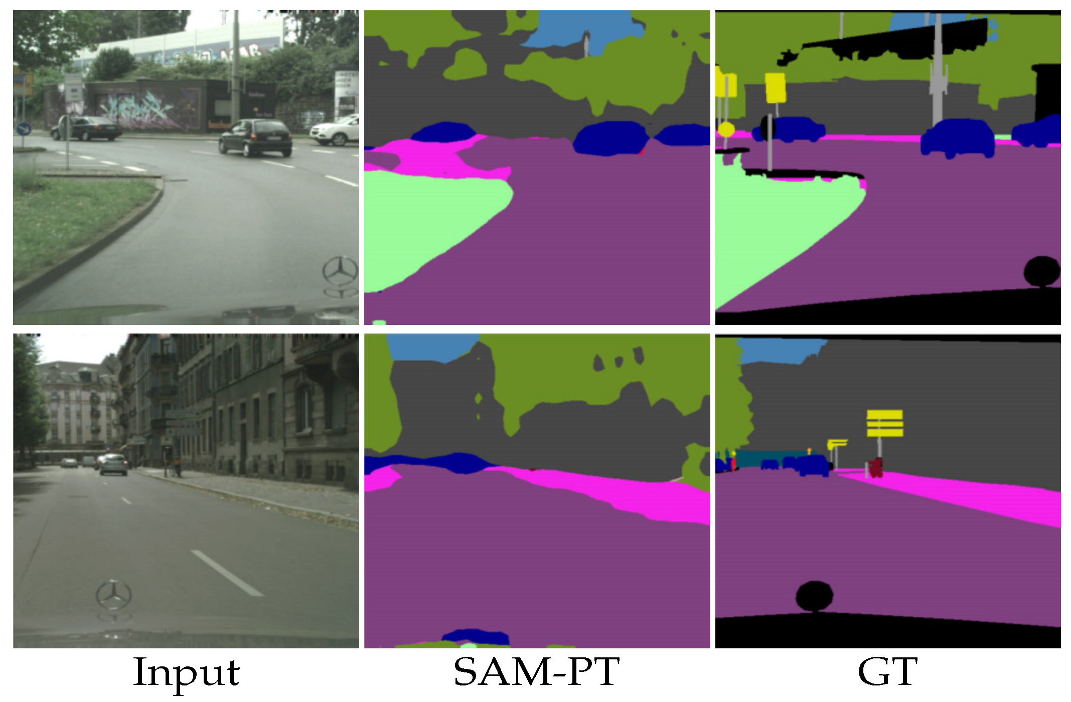
However, SAM’s segmentation results lack semantic information, and its performance is not strong enough in adverse-condition environments [74]. Painter [38] suffers from severe over-fitting. We attempted to use the semantic segmentation labels from the ACDC dataset as the task prompt, but Painter produced an output for the depth estimation instead. Therefore, it is challenging for large-scale models to surpass those specialized domain models in a short period. Moreover, transferring large-scale models to proprietary task label systems is both time consuming and difficult. Taking SAM as an example, it is trained using the ViT [75] series framework (because ViT is naturally suitable for pretraining in masked image modeling [58]). We tried both fine-tuning and prompt tuning [39] for adapting to Citsycapes, but it was difficult (it only reached 18% mIoU after 40,000 iterations, while SegFormer [57] easily achieves 75%+), and SAM’s fine-tuning was easily bottlenecked due to the limited volume of Cityscapes. This indicates that the built-in segmentation knowledge in SAM does not help the model smoothly migrate to the current high-level domain. On the other hand, ViT-based models are inferior to SegFormer in terms of speed and memory consumption (as shown in Table 9). SegFormer only requires 6–8 GB of memory for testing, while ViT-based models require 15–20 GB (batch_size = 1). Additionally, SegFormer-based models significantly outperform ViT-based models in testing speed (6–7 FPS vs. 1–2 FPS). Therefore, we have decided to use a SegFormer-based model instead of fine-tuning (or prompt tuning) a large-scale model.

5.8. Limitations

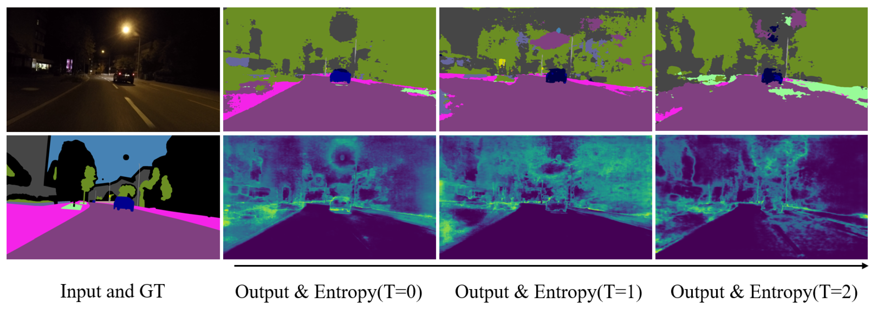
Although the USP method proposed in this paper achieves good performance in the adaptation task during testing, there are also some failure cases. The most typical example of them comes in the dark. As shown in Figure 12, we give the test results from the first round to the third round of adaptation. It can be seen that the test results of these three rounds gradually deteriorate, and the overall entropy distribution becomes worse and worse. This is because the segmentation of the night scene has already brought higher entropy even in the initial state (T = 0), while USP is directly dependent on entropy to explore the domain gap, which leads to the inevitable error accumulation in the exploration process of the model. This problem is also due to the inherent difficulty of the semantic segmentation during nighttime, needing to be further processed.

6. Conclusions

We propose a test-time adaptation framework based on uncertainty, named USP, which utilizes a teacher–student paradigm along with separating the consistency learning process to achieve better robustness. USP employs entropy as a measure of uncertainty to capture areas within consecutive images that exhibit domain gaps, and then self-prompts the model, guiding the latter to explore new knowledge. In the prompt process, we designed a prompt module and a random dropout strategy to mitigate model over-fitting and catastrophic forgetting. To capture temporal information, we also devised an uncertainty-based prompt module updating method that relies on total entropy.
Experimental results demonstrate that the prompt module can effectively integrate information from the entropy and raw images, making reasonable adjustments to the model’s attention. Our approach outperforms current TTA algorithms on mainstream datasets like ACDC and Foggy and Rainy Cityscapes. Ablation studies confirm that the teacher–student module, uncertainty self-prompt module, domain prompt update strategy, and random dropout strategy all contribute to the model’s robustness. We further explored the hyper-parameters of dropout probability and threshold through ablation experiments to ascertain their optimal values. In addition, we analyzed the role of test-time data augmentation strategies, showing that data augmentation could simulate real domain discrepancies to some extent. Lastly, we compared our method with currently popular large-scale pretrained semantic segmentation networks, elucidating the reasons for not fine-tuning these models. Our method is capable of mining information from unlabeled data and combating forgetting, exhibiting good robustness and adaptability. In the future research, we will pay more attention to the knowledge related to large models and better utilize prompt techniques in TTA.
There are still some limitations in this study. Our research is still within the TTA framework, requiring complex test-time augmentation operation, which greatly slows down the running speed. Our method is also less effective when dealing with scenes with high initial entropy, such as night. In future studies, we will try to improve the running speed of the algorithm.

Author Contributions

Conceptualization, Z.W., Z.Z. and Z.J; methodology, Z.W. and Z.J.; software, Z.W. and Z.J.; validation, Z.W., Y.Z. and Y.Y.; formal analysis, Y.Z., L.L. and L.Z.; investigation, Z.W., Y.Y. and L.L.; data curation., Z.J., Y.Y., L.L. and L.Z.; writing—original draft preparation, Z.W., Z.Z., Z.J. and L.Z.; writing—review and editing, Z.W., Z.J., L.L. and L.Z.; visualization, Z.Z. and Y.Z.; supervision, Y.Z.; project administration, Y.Z.; funding acquisition, Y.Z. and Y.Y. All authors have read and agreed to the published version of the manuscript.

Funding

This work was supported by the National Natural Science Foundation of China under Grant 42071340 and the Program of Song Shan Laboratory (included in the management of Major Science and Technology of Henan Province) under Grant 2211000211000-01.

Data Availability Statement

The original contributions presented in the study are included in the article, further inquiries can be directed to the corresponding author.

Acknowledgments

In the process of our research, Song Ji put forward valuable suggestions for the experiments; we would like to express our thanks here. We also thank Binbin Cheng for his efforts in the late proofreading and polishing of the paper.

Conflicts of Interest

The authors declare no conflicts of interest.

Nomenclature

Acronyms list:
Nomenclature
DADomain AdaptationDPUDomain Prompt Updating
DGDomain GeneralizationUSPUncertainty-based Self-Prompt
TTATest-Time AdaptationVPTVisual Prompt Tuning
CTTAContinual Test-Time AdaptationGTGround Truth
VDPVisual Domain PromptACDCAdverse Condition Datasets with Correspondence

References

  1. Zhu, H.; Yuen, K.V.; Mihaylova, L.; Leung, H. Overview of Environment Perception for Intelligent Vehicles. IEEE Trans. Intell. Transp. Syst. 2017, 18, 2584–2601. [Google Scholar] [CrossRef]
  2. Kuutti, S.; Bowden, R.; Jin, Y.; Barber, P.; Fallah, S. A Survey of Deep Learning Applications to Autonomous Vehicle Control. IEEE Trans. Intell. Transp. Syst. 2021, 22, 712–733. [Google Scholar] [CrossRef]
  3. Feng, D.; Haase-Schütz, C.; Rosenbaum, L.; Hertlein, H.; Gläser, C.; Timm, F.; Wiesbeck, W.; Dietmayer, K. Deep Multi-Modal Object Detection and Semantic Segmentation for Autonomous Driving: Datasets, Methods, and Challenges. IEEE Trans. Intell. Transp. Syst. 2021, 22, 1341–1360. [Google Scholar] [CrossRef]
  4. Zhang, J.; Pu, J.; Chen, J.; Fu, H.; Tao, Y.; Wang, S.; Chen, Q.; Xiao, Y.; Chen, S.; Cheng, Y.; et al. DSiV: Data Science for Intelligent Vehicles. IEEE Trans. Intell. Veh. 2023, 8, 2628–2634. [Google Scholar] [CrossRef]
  5. Ranft, B.; Stiller, C. The Role of Machine Vision for Intelligent Vehicles. IEEE Trans. Intell. Veh. 2016, 1, 8–19. [Google Scholar] [CrossRef]
  6. Muhammad, K.; Hussain, T.; Ullah, H.; Ser, J.D.; Rezaei, M.; Kumar, N.; Hijji, M.; Bellavista, P.; de Albuquerque, V.H.C. Vision-Based Semantic Segmentation in Scene Understanding for Autonomous Driving: Recent Achievements, Challenges, and Outlooks. IEEE Trans. Intell. Transp. Syst. 2022, 23, 22694–22715. [Google Scholar] [CrossRef]
  7. Sakaridis, C.; Dai, D.; Van Gool, L. Semantic foggy scene understanding with synthetic data. Int. J. Comput. Vis. 2018, 126, 973–992. [Google Scholar] [CrossRef]
  8. Dai, D.; Gool, L.V. Dark Model Adaptation: Semantic Image Segmentation from Daytime to Nighttime. In Proceedings of the 2018 21st International Conference on Intelligent Transportation Systems (ITSC), Maui, HI, USA, 4–7 November 2018. [Google Scholar]
  9. Sakaridis, C.; Dai, D.; Gool, L.V. ACDC: The adverse conditions dataset with correspondences for semantic driving scene understanding. In Proceedings of the IEEE/CVF International Conference on Computer Vision, Montreal, BC, Canada, 11–17 October 2021; pp. 10765–10775. [Google Scholar]
  10. Hoyer, L.; Dai, D.; Van Gool, L. Daformer: Improving network architectures and training strategies for domain-adaptive semantic segmentation. In Proceedings of the IEEE/CVF Conference on Computer Vision and Pattern Recognition, New Orleans, LA, USA, 18–24 June 2022; pp. 9924–9935. [Google Scholar]
  11. Tsai, Y.H.; Hung, W.C.; Schulter, S.; Sohn, K.; Yang, M.H.; Chandraker, M. Learning to adapt structured output space for semantic segmentation. In Proceedings of the IEEE Conference on Computer Vision and Pattern Recognition, Salt Lake City, UT, USA, 18–23 June 2018; pp. 7472–7481. [Google Scholar]
  12. Vu, T.H.; Jain, H.; Bucher, M.; Cord, M.; Pérez, P. Advent: Adversarial entropy minimization for domain adaptation in semantic segmentation. In Proceedings of the IEEE/CVF Conference on Computer Vision and Pattern Recognition, Long Beach, CA, USA, 15–20 June 2019; pp. 2517–2526. [Google Scholar]
  13. Li, Y.; Yuan, L.; Vasconcelos, N. Bidirectional learning for domain adaptation of semantic segmentation. In Proceedings of the IEEE/CVF Conference on Computer Vision and Pattern Recognition, Long Beach, CA, USA, 15–20 June 2019; pp. 6936–6945. [Google Scholar]
  14. Zou, Y.; Yu, Z.; Liu, X.; Kumar, B.V.; Wang, J. Confidence Regularized Self-Training. In Proceedings of the IEEE International Conference on Computer Vision (ICCV), Seoul, Republic of Korea, 27 October–2 November 2019. [Google Scholar]
  15. Tranheden, W.; Olsson, V.; Pinto, J.; Svensson, L. Dacs: Domain adaptation via cross-domain mixed sampling. In Proceedings of the IEEE/CVF Winter Conference on Applications of Computer Vision, Virtual, 5–9 January 2021; pp. 1379–1389. [Google Scholar]
  16. Ma, X.; Wang, Z.; Zhan, Y.; Zheng, Y.; Wang, Z.; Dai, D.; Lin, C.W. Both style and fog matter: Cumulative domain adaptation for semantic foggy scene understanding. In Proceedings of the IEEE/CVF Conference on Computer Vision and Pattern Recognition, New Orleans, LA, USA, 18–24 June 2022; pp. 18922–18931. [Google Scholar]
  17. Hoyer, L.; Dai, D.; Van Gool, L. HRDA: Context-aware high-resolution domain-adaptive semantic segmentation. In Proceedings of the European Conference on Computer Vision, Tel Aviv, Israel, 23–27 October 2022; Springer: Berlin/Heidelberg, Germany, 2022; pp. 372–391. [Google Scholar]
  18. Hoyer, L.; Dai, D.; Wang, H.; Gool, L.V. MIC: Masked Image Consistency for Context-Enhanced Domain Adaptation. arXiv 2023, arXiv:2212.01322. [Google Scholar]
  19. Muandet, K.; Balduzzi, D.; Schölkopf, B. Domain generalization via invariant feature representation. In Proceedings of the International Conference on Machine Learning, Atlanta, GA, USA, 16–21 June 2013; pp. 10–18. [Google Scholar]
  20. Li, B.; Wu, F.; Lim, S.N.; Belongie, S.; Weinberger, K.Q. On feature normalization and data augmentation. In Proceedings of the IEEE/CVF Conference on Computer Vision and Pattern Recognition, Nashville, TN, USA, 20–25 June 2021; pp. 12383–12392. [Google Scholar]
  21. Yin, D.; Gontijo Lopes, R.; Shlens, J.; Cubuk, E.D.; Gilmer, J. A fourier perspective on model robustness in computer vision. In Advances in Neural Information Processing Systems; MiT and Morgan Kaufmann: San Francisco, CA, USA, 2019; Volume 32. [Google Scholar]
  22. Ashukha, A.; Lyzhov, A.; Molchanov, D.; Vetrov, D. Pitfalls of in-domain uncertainty estimation and ensembling in deep learning. arXiv 2020, arXiv:2002.06470. [Google Scholar]
  23. Lyzhov, A.; Molchanova, Y.; Ashukha, A.; Molchanov, D.; Vetrov, D. Greedy policy search: A simple baseline for learnable test-time augmentation. In Proceedings of the Conference on Uncertainty in Artificial Intelligence, Virtual, 3–6 August 2020; pp. 1308–1317. [Google Scholar]
  24. Tobin, J.; Fong, R.; Ray, A.; Schneider, J.; Zaremba, W.; Abbeel, P. Domain randomization for transferring deep neural networks from simulation to the real world. In Proceedings of the 2017 IEEE/RSJ International Conference on Intelligent Robots and Systems (IROS), Vancouver, BC, Canada, 24–28 September 2017; pp. 23–30. [Google Scholar]
  25. Tremblay, J.; Prakash, A.; Acuna, D.; Brophy, M.; Jampani, V.; Anil, C.; To, T.; Cameracci, E.; Boochoon, S.; Birchfield, S. Training deep networks with synthetic data: Bridging the reality gap by domain randomization. In Proceedings of the IEEE Conference on Computer Vision and Pattern Recognition Workshops, Salt Lake City, UT, USA, 18–23 June 2018; pp. 969–977. [Google Scholar]
  26. Liang, J.; He, R.; Tan, T. A Comprehensive Survey on Test-Time Adaptation under Distribution Shifts. arXiv 2023, arXiv:2303.15361. [Google Scholar]
  27. Mummadi, C.K.; Hutmacher, R.; Rambach, K.; Levinkov, E.; Brox, T.; Metzen, J.H. Test-Time Adaptation to Distribution Shift by Confidence Maximization and Input Transformation. arXiv 2021, arXiv:2106.14999. [Google Scholar]
  28. Wang, D.; Shelhamer, E.; Liu, S.; Olshausen, B.; Darrell, T. Tent: Fully Test-time Adaptation by Entropy Minimization. arXiv 2021, arXiv:2006.10726. [Google Scholar]
  29. Liang, J.; Hu, D.; Feng, J. Do We Really Need to Access the Source Data? Source Hypothesis Transfer for Unsupervised Domain Adaptation. In Proceedings of the 37th International Conference on Machine Learning, Virtual, 13–18 July 2020. JMLR.org, ICML’20. [Google Scholar]
  30. Liu, Y.; Zhang, W.; Wang, J. Source-Free Domain Adaptation for Semantic Segmentation. arXiv 2021, arXiv:2103.16372. [Google Scholar]
  31. Ye, M.; Zhang, J.; Ouyang, J.; Yuan, D. Source Data-Free Unsupervised Domain Adaptation for Semantic Segmentation. In Proceedings of the 29th ACM International Conference on Multimedia, Virtual, 20–24 October 2021; Association for Computing Machinery: New York, NY, USA, 2021. MM ’21. pp. 2233–2242. [Google Scholar] [CrossRef]
  32. Wang, Q.; Fink, O.; Van Gool, L.; Dai, D. Continual test-time domain adaptation. In Proceedings of the IEEE/CVF Conference on Computer Vision and Pattern Recognition, New Orleans, LA, USA, 18–24 June 2022; pp. 7201–7211. [Google Scholar]
  33. Ioffe, S.; Szegedy, C. Batch Normalization: Accelerating Deep Network Training by Reducing Internal Covariate Shift. In Proceedings of the 32nd International Conference on International Conference on Machine Learning—Volume 37, Lille, France, 7–9 July 2015; JMLR.org, ICML’15. pp. 448–456. [Google Scholar]
  34. Tarvainen, A.; Valpola, H. Mean teachers are better role models: Weight-averaged consistency targets improve semi-supervised deep learning results. In Advances in Neural Information Processing Systems; MiT and Morgan Kaufmann: San Francisco, CA, USA, 2017; Volume 30. [Google Scholar]
  35. Li, Z.; Hoiem, D. Learning without forgetting. IEEE Trans. Pattern Anal. Mach. Intell. 2017, 40, 2935–2947. [Google Scholar] [CrossRef]
  36. Brown, T.; Mann, B.; Ryder, N.; Subbiah, M.; Kaplan, J.D.; Dhariwal, P.; Neelakantan, A.; Shyam, P.; Sastry, G.; Askell, A.; et al. Language models are few-shot learners. Adv. Neural Inf. Process. Syst. 2020, 33, 1877–1901. [Google Scholar]
  37. Kirillov, A.; Mintun, E.; Ravi, N.; Mao, H.; Rolland, C.; Gustafson, L.; Xiao, T.; Whitehead, S.; Berg, A.C.; Lo, W.Y.; et al. Segment Anything. arXiv 2023, arXiv:2304.02643. [Google Scholar]
  38. Wang, X.; Wang, W.; Cao, Y.; Shen, C.; Huang, T. Images speak in images: A generalist painter for in-context visual learning. In Proceedings of the IEEE/CVF Conference on Computer Vision and Pattern Recognition, Vancouver, BC, Canada, 17–24 June 2023; pp. 6830–6839. [Google Scholar]
  39. Jia, M.; Tang, L.; Chen, B.C.; Cardie, C.; Belongie, S.; Hariharan, B.; Lim, S.N. Visual prompt tuning. In Proceedings of the European Conference on Computer Vision, Tel Aviv, Israel, 23–27 October 2022; Springer: Berlin/Heidelberg, Germany, 2022; pp. 709–727. [Google Scholar]
  40. Gan, Y.; Bai, Y.; Lou, Y.; Ma, X.; Zhang, R.; Shi, N.; Luo, L. Decorate the newcomers: Visual domain prompt for continual test time adaptation. In Proceedings of the AAAI Conference on Artificial Intelligence, Washington, DC, USA, 7–14 February 2023; Volume 37, pp. 7595–7603. [Google Scholar]
  41. Gao, Y.; Shi, X.; Zhu, Y.; Wang, H.; Tang, Z.; Zhou, X.; Li, M.; Metaxas, D.N. Visual prompt tuning for test-time domain adaptation. arXiv 2022, arXiv:2210.04831. [Google Scholar]
  42. Ge, C.; Huang, R.; Xie, M.; Lai, Z.; Song, S.; Li, S.; Huang, G. Domain adaptation via prompt learning. arXiv 2022, arXiv:2202.06687. [Google Scholar] [CrossRef] [PubMed]
  43. Cordts, M.; Omran, M.; Ramos, S.; Rehfeld, T.; Enzweiler, M.; Benenson, R.; Franke, U.; Roth, S.; Schiele, B. The cityscapes dataset for semantic urban scene understanding. In Proceedings of the IEEE Conference on Computer Vision and Pattern Recognition, Las Vegas, NV, USA, 27–30 June 2016; pp. 3213–3223. [Google Scholar]
  44. Dai, Y.; Li, C.; Su, X.; Liu, H.; Li, J. Multi-Scale Depthwise Separable Convolution for Semantic Segmentation in Street–Road Scenes. Remote Sens. 2023, 15, 2649. [Google Scholar] [CrossRef]
  45. Li, X.; Xu, F.; Lyu, X.; Gao, H.; Tong, Y.; Cai, S.; Li, S.; Liu, D. Dual attention deep fusion semantic segmentation networks of large-scale satellite remote-sensing images. Int. J. Remote Sens. 2021, 42, 3583–3610. [Google Scholar] [CrossRef]
  46. Hehn, T.; Kooij, J.; Gavrila, D. Fast and Compact Image Segmentation Using Instance Stixels. IEEE Trans. Intell. Veh. 2022, 7, 45–56. [Google Scholar] [CrossRef]
  47. Ni, P.; Li, X.; Kong, D.; Yin, X. Scene-Adaptive 3D Semantic Segmentation Based on Multi-Level Boundary-Semantic-Enhancement for Intelligent Vehicles. IEEE Trans. Intell. Veh. 2023, 9, 1722–1732. [Google Scholar] [CrossRef]
  48. Liu, Q.; Dong, Y.; Jiang, Z.; Pei, Y.; Zheng, B.; Zheng, L.; Fu, Z. Multi-Pooling Context Network for Image Semantic Segmentation. Remote Sens. 2023, 15, 2800. [Google Scholar] [CrossRef]
  49. Sun, Q.; Chao, J.; Lin, W.; Xu, Z.; Chen, W.; He, N. Learn to Few-Shot Segment Remote Sensing Images from Irrelevant Data. Remote Sens. 2023, 15, 4937. [Google Scholar] [CrossRef]
  50. Richter, S.R.; Vineet, V.; Roth, S.; Koltun, V. Playing for data: Ground truth from computer games. In Proceedings of the Computer Vision—ECCV 2016: 14th European Conference, Amsterdam, The Netherlands, 11–14 October 2016; Part II 14. Springer: Berlin/Heidelberg, Germany, 2016; pp. 102–118. [Google Scholar]
  51. Ros, G.; Sellart, L.; Materzynska, J.; Vazquez, D.; Lopez, A.M. The synthia dataset: A large collection of synthetic images for semantic segmentation of urban scenes. In Proceedings of the IEEE Conference on Computer Vision and Pattern Recognition, Las Vegas, NV, USA, 27–30 June 2016; pp. 3234–3243. [Google Scholar]
  52. Hoffman, J.; Wang, D.; Yu, F.; Darrell, T. Fcns in the wild: Pixel-level adversarial and constraint-based adaptation. arXiv 2016, arXiv:1612.02649. [Google Scholar]
  53. Goodfellow, I.; Pouget-Abadie, J.; Mirza, M.; Xu, B.; Warde-Farley, D.; Ozair, S.; Courville, A.; Bengio, Y. Generative adversarial networks. Commun. ACM 2020, 63, 139–144. [Google Scholar] [CrossRef]
  54. Hoffman, J.; Tzeng, E.; Park, T.; Zhu, J.Y.; Isola, P.; Saenko, K.; Efros, A.A.; Darrell, T. CyCADA: Cycle-Consistent Adversarial Domain Adaptation. arXiv 2017, arXiv:1711.03213. [Google Scholar]
  55. Chang, W.L.; Wang, H.P.; Peng, W.H.; Chiu, W.C. All about structure: Adapting structural information across domains for boosting semantic segmentation. In Proceedings of the IEEE/CVF Conference on Computer Vision and Pattern Recognition, Long Beach, CA, USA, 16–17 June 2019; pp. 1900–1909. [Google Scholar]
  56. Zhang, P.; Zhang, B.; Zhang, T.; Chen, D.; Wang, Y.; Wen, F. Prototypical pseudo label denoising and target structure learning for domain adaptive semantic segmentation. In Proceedings of the IEEE/CVF Conference on Computer Vision and Pattern Recognition, Nashville, TN, USA, 20–25 June 2021; pp. 12414–12424. [Google Scholar]
  57. Xie, E.; Wang, W.; Yu, Z.; Anandkumar, A.; Alvarez, J.M.; Luo, P. SegFormer: Simple and efficient design for semantic segmentation with transformers. Adv. Neural Inf. Process. Syst. 2021, 34, 12077–12090. [Google Scholar]
  58. He, K.; Chen, X.; Xie, S.; Li, Y.; Dollár, P.; Girshick, R. Masked autoencoders are scalable vision learners. In Proceedings of the IEEE/CVF Conference on Computer Vision and Pattern Recognition, New Orleans, LA, USA, 18–24 June 2022; pp. 16000–16009. [Google Scholar]
  59. Michieli, U.; Biasetton, M.; Agresti, G.; Zanuttigh, P. Adversarial Learning and Self-Teaching Techniques for Domain Adaptation in Semantic Segmentation. IEEE Trans. Intell. Veh. 2020, 5, 508–518. [Google Scholar] [CrossRef]
  60. De Lange, M.; Aljundi, R.; Masana, M.; Parisot, S.; Jia, X.; Leonardis, A.; Slabaugh, G.; Tuytelaars, T. A continual learning survey: Defying forgetting in classification tasks. IEEE Trans. Pattern Anal. Mach. Intell. 2021, 44, 3366–3385. [Google Scholar]
  61. Huang, J.; Guan, D.; Xiao, A.; Lu, S. Model Adaptation: Historical Contrastive Learning for Unsupervised Domain Adaptation without Source Data. arXiv 2022, arXiv:2110.03374. [Google Scholar]
  62. Rebuffi, S.A.; Kolesnikov, A.; Sperl, G.; Lampert, C.H. iCaRL: Incremental Classifier and Representation Learning. arXiv 2017, arXiv:1611.07725. [Google Scholar]
  63. Bar, A.; Gandelsman, Y.; Darrell, T.; Globerson, A.; Efros, A. Visual prompting via image inpainting. Adv. Neural Inf. Process. Syst. 2022, 35, 25005–25017. [Google Scholar]
  64. Yang, S.; Wu, J.; Liu, J.; Li, X.; Zhang, Q.; Pan, M.; Pan, M.; Zhang, S. Exploring Sparse Visual Prompt for Cross-domain Semantic Segmentation. arXiv 2023, arXiv:2303.09792. [Google Scholar]
  65. Laine, S.; Aila, T. Temporal ensembling for semi-supervised learning. arXiv 2016, arXiv:1610.02242. [Google Scholar]
  66. Shannon, C.E. A Mathematical Theory of Communication. Bell Syst. Tech. J. 1948, 27, 623–656. [Google Scholar] [CrossRef]
  67. Romera, E.; Álvarez, J.M.; Bergasa, L.M.; Arroyo, R. ERFNet: Efficient Residual Factorized ConvNet for Real-Time Semantic Segmentation. IEEE Trans. Intell. Transp. Syst. 2018, 19, 263–272. [Google Scholar] [CrossRef]
  68. Chen, B.; Gong, C.; Yang, J. Importance-Aware Semantic Segmentation for Autonomous Vehicles. IEEE Trans. Intell. Transp. Syst. 2019, 20, 137–148. [Google Scholar] [CrossRef]
  69. Fan, J.; Wang, F.; Chu, H.; Hu, X.; Cheng, Y.; Gao, B. MLFNet: Multi-Level Fusion Network for Real-Time Semantic Segmentation of Autonomous Driving. IEEE Trans. Intell. Veh. 2023, 8, 756–767. [Google Scholar] [CrossRef]
  70. Chen, C.; Wang, C.; Liu, B.; He, C.; Cong, L.; Wan, S. Edge Intelligence Empowered Vehicle Detection and Image Segmentation for Autonomous Vehicles. IEEE Trans. Intell. Transp. Syst. 2023, 24, 13023–13034. [Google Scholar] [CrossRef]
  71. Contributors, M. MMSegmentation: Openmmlab Semantic Segmentation Toolbox and Benchmark. 2020. Available online: https://github.com/open-mmlab/mmsegmentation (accessed on 22 January 2024).
  72. Kingma, D.P.; Ba, J. Adam: A method for stochastic optimization. arXiv 2014, arXiv:1412.6980. [Google Scholar]
  73. Wang, X.; Zhang, X.; Cao, Y.; Wang, W.; Shen, C.; Huang, T. SegGPT: Segmenting Everything In Context. arXiv 2023, arXiv:2304.03284. [Google Scholar]
  74. Wang, Z.; Zhang, Y.; Ma, X.; Yu, Y.; Zhang, Z.; Jiang, Z.; Cheng, B. Semantic Segmentation of Foggy Scenes Based on Progressive Domain Gap Decoupling 2023. Available online: https://www.techrxiv.org/doi/full/10.36227/techrxiv.22682161.v1 (accessed on 22 January 2024).
  75. Dosovitskiy, A.; Beyer, L.; Kolesnikov, A.; Weissenborn, D.; Zhai, X.; Unterthiner, T.; Dehghani, M.; Minderer, M.; Heigold, G.; Gelly, S.; et al. An Image is Worth 16 × 16 Words: Transformers for Image Recognition at Scale. arXiv 2021, arXiv:2010.11929. [Google Scholar]
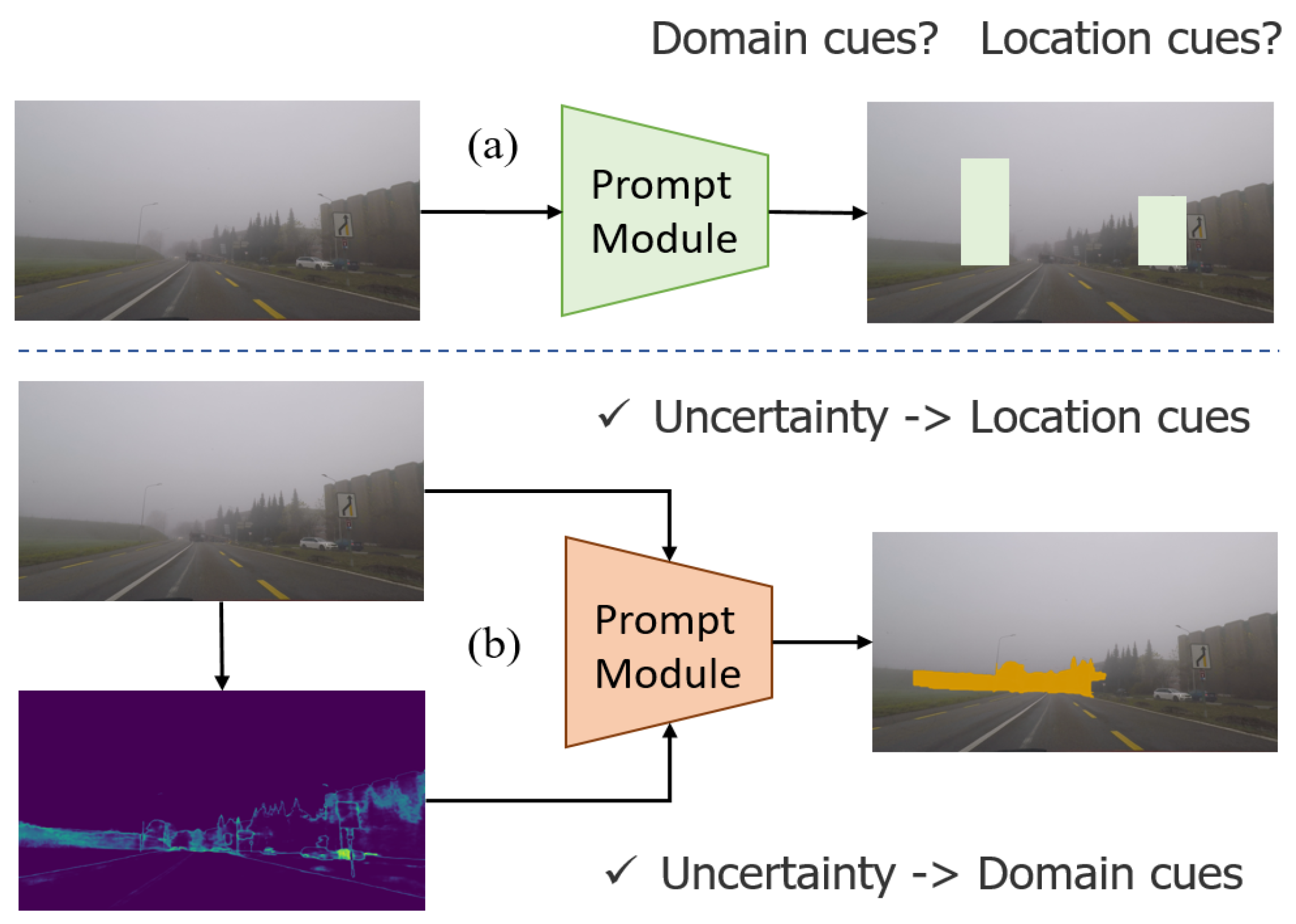
Figure 1. The main idea of proposed method. In The different colors here represent different types of prompt modules and the distribution of prompt values in the image. The original Visual Domain Prompt method shown in (a), the prompt does not provide explicit location information and meaning, making it difficult to interpret. We proposes a self-prompting strategy based on uncertainty shown in (b). It utilizes regions with high uncertainty as prompts for identifying domain gaps and guides the model to cross the domain. Thus, the domain prompt possess explicit regional meanings and domain cues.
Remotesensing 16 01239 g001
Figure 2. The overall pipeline. (a) The training TTA with uncertainty-based self-prompt. (b) The testing TTA pipeline. The prompt module will process the entropy of the segmentor and re-input the prompted image. The blue lines represent the data flows and modules related to the teacher model, the green lines represent the data flows and modules related to the student model, and the yellow lines indicate the data flows of the modules.
Remotesensing 16 01239 g002
Figure 3. Domain prompt updating.
Remotesensing 16 01239 g003
Figure 4. Experiment workflow.
Remotesensing 16 01239 g004
Figure 5. Performance comparison. We conduct test-time adaptation on the ACDC [9] dataset. Color blocks are assigned according to Cityscapes benchmark. The scenes from top to bottom are foggy, rainy, snowy, and nighttime, respectively. Intuitively, our method can better recognize sidewalks in the images, which is valuable for autonomous driving. Additionally, in the rain images with more noise, our method exhibits stronger anti-interference capability and produces less uncertainty in the segmentation results.
Remotesensing 16 01239 g005
Figure 6. Ablation of dropout probability p. Here, the performance will peak when p = 0.5 . When p 0 or p 1 , the performance degrades to baseline.
Remotesensing 16 01239 g006
Figure 7. Ablation of dropout threshold τ . When fixing p = 0.5 , the performance will peak at 0.85. When τ 1 , the performance still remains high.
Remotesensing 16 01239 g007
Figure 8. Visual effect of prompt. After the entropy map generated by the teacher model, the prompt module will process and attach it to the input. The yellow box line marks the change of attention of the prompt module to entropy processing, while the red box line marks the visual effect of the prompt module combined with the original image.
Remotesensing 16 01239 g008
Figure 9. Impact of USP to attention of model. The predictive entropy and attention maps output by models trained with and without the USP method. The model trained using USP has lower entropy and a more even distribution of attention, thereby indicating the model has better generalization.
Remotesensing 16 01239 g009
Figure 10. Augmentation examples. We set six scaling parameters to produce images of various sizes and randomly applied four types of data augmentation techniques at each scale.
Remotesensing 16 01239 g010
Figure 11. Performance of prompt-tuning SAM.
Remotesensing 16 01239 g011
Figure 12. Failure case in the three round of continuous TTA process. Color blocks are assigned according to Cityscapes benchmark. For the entropy maps, the brighter the color, the higher the value at that pixel.
Remotesensing 16 01239 g012
Table 1. The datasets used.
DatasetScenarioLabelled ImagesNumber of Label UsedExperiment Purpose
CityscapesAutonomous Driving in clear scene2975(train)/500(val)2975(for train source)not involved in testing
Foggy CityscapesAutonomous Driving in synthetic foggy scene2975(train)/500(val)0(TTA)/2975(for evaluation)Test the performance of TTA
Rainy CityscapesAutonomous Driving in synthetic rainy scene2975(train)/500(val)0(TTA)/2975(for evaluation)Test the performance of TTA
ACDC-FogAutonomous Driving in real foggy scene400(train)/100(val)0(TTA)/400(for evaluation)Test the performance of TTA
ACDC-RainAutonomous Driving in real rainy scene400(train)/100(val)0(TTA)/400(for evaluation)Test the performance of TTA
ACDC-NightAutonomous Driving in real nighttime scene400(train)/106(val)0(TTA)/400(for evaluation)Test the performance of TTA
ACDC-SnowAutonomous Driving in real snowy scene400(train)/100(val)0(TTA)/400(for evaluation)Test the performance of TTA
Table 2. Performance comparison of Cityscapes-to-ACDC TTA. We use Cityscape as the source domain and ACDC as the four target domains in this setting. Source domain data are unavailable, while target domain data are only accessed once during testing. The best performance data is shown in bold.
Test-Time AdaptationSource2FogSource2NightSource2RainSource2SnowMean-mIoU↑
MethodREFmIoU↑mAcc↑mIoU↑mAcc↑mIoU↑mAcc↑mIoU↑mAcc↑
ERFNetTITS2018 [67]61.371.128.441.647.661.051.862.747.3
IALTITS2019 [68]64.074.834.546.352.867.254.066.451.3
SegFormerNeurIPS2021 [57]69.179.440.355.659.774.457.869.956.7
TENTICLR2021 [28]69.079.540.355.559.973.257.769.756.7
CoTTACVPR2022 [32]70.980.241.255.562.675.459.870.758.6
MLFNetTIV2023 [69]68.477.339.254.160.872.356.368.256.2
EIETITS2023 [70]70.279.140.555.060.272.158.670.357.4
DePTICLR2023 [41]71.080.240.955.861.374.459.570.058.2
VDPAAAI2023 [40]70.980.341.255.662.375.559.770.758.5
SVDPICCV2023 [64]72.581.445.358.965.776.762.272.461.4
USPOurs73.282.144.959.466.477.063.272.861.9
Table 3. Performance comparison for Cityscape-to-ACDC CTTA. We take the Cityscape as the source domain and ACDC as the fourtarget domains. During testing, we sequentially evaluate the four target domains multiple times. Mean is the average score of mIoU for all times. Gain refers to the improvement achieved by the method compared to the source model. The best performance data is shown in bold.
Timet————————————————————————————————>
Round123MeanGain
MethodREFFogNightRainSnowMeanFogNightRainSnowMeanFogNightRainSnowMean
ERFNetTITS2018 [67]61.228.447.551.847.261.228.447.551.847.261.228.447.551.847.247.2-
IALTITS2019 [68]64.034.452.854.051.364.034.452.854.051.364.034.452.854.051.351.3-
MLFNetTIV2023 [69]68.439.360.956.356.268.439.360.956.356.268.439.360.956.356.256.2-
EIETITS2023 [70]70.140.360.358.557.370.140.360.358.557.370.140.360.358.557.357.3-
SegFormerNeurIPS2021 [57]69.140.359.757.856.769.140.359.757.856.769.140.359.757.856.756.7-
TENTICLR2021 [28]69.040.260.157.356.768.339.060.156.355.967.537.859.655.055.055.7-1.0
CoTTACVPR2022 [32]70.941.262.459.758.670.941.162.659.758.670.941.062.759.758.658.6+1.9
DePTICLR2023 [41]71.040.858.256.856.568.240.055.453.754.366.438.047.347.249.753.4-3.3
VDPAAAI2023 [40]70.541.162.159.558.370.441.162.259.458.270.441.062.259.458.258.2+1.5
SVDPICCV2023 [64]72.545.967.064.162.472.244.867.364.162.172.044.567.664.262.162.2+5.5
USPOurs74.244.667.464.562.774.144.667.364.262.574.144.667.063.862.362.5+5.8
Table 4. Comparison of performance between models trained with USP and without USP on the four target domains. The best performance data is shown in bold.
SkyRoadBuildVeget.TrainCarTerrainTruckS.walkRiderTr.SingTr.LightBusM.BikeWallPersonPoleBikeFencemIoU
S2Fogw/o USP98.190.688.384.382.689.473.577.980.476.979.369.478.655.860.159.949.330.323.370.9
w/ USP98.893.587.281.488.992.677.480.179.581.280.175.277.156.963.460.244.740.832.573.2
S2Nightw/o USP37.976.468.365.732.972.138.415.350.320.356.735.442.926.46.6054.438.333.810.241.2
w/ USP44.675.179.248.350.368.941.226.450.125.237.015.840.331.529.455.937.147.618.344.9
S2Rainw/o USP96.483.185.492.676.584.341.865.945.422.167.362.458.749.744.757.752.156.347.562.6
w/ USP97.988.290.491.079.488.943.061.055.445.362.162.482.342.860.358.951.857.041.066.3
S2Snoww/o USP94.781.383.789.478.387.810.354.949.843.164.265.451.937.535.364.147.057.140.859.8
w/ USP96.984.184.285.387.188.925.653.537.455.362.470.374.139.228.561.651.361.753.263.2
Table 5. Cityscapes to (Foggy and Rainy) Cityscapes TTA performance comparison. The best performance data is shown in bold.
FoggySegFormerTENTCoTTADePTVDPSVDPUSP
mIoU69.269.372.171.971.874.576.2
mAcc79.179.079.480.280.082.384.3
RainySegFormerTENTCoTTADePTVDPSVDPUSP
mIoU58.458.762.461.263.765.365.3
mAcc71.571.474.072.473.175.677.7
Table 6. Ablation: ✓ indicates that the component is being used in the current experiment. Contribution of each component.
TS 1USP 2DPU 3P-Drop 4mIoUmAcc
E x 1 69.179.4
E x 2 69.479.6
E x 3 72.481.2
E x 4 72.981.2
E x 5 73.081.8
E x 6 73.282.1
1 teacher–student framework. 2 uncertainty-based prompt. 3 domain prompt updating. 4 prompt dropout.
Table 7. The effect of different prompt module architecture. We design four prompt modules with different number of parameters.
Prompt Module
City-to-ACDC(fog) TTA
Architecture
Prompt|SPrompt|MPrompt|LPrompt|H
Encoder Conv 3 × 3 8 Conv 3 × 3 32 Conv 3 × 3 8 Conv 3 × 3 32 Conv 3 × 3 64 Conv 3 × 3 8 Conv 3 × 3 32 Conv 3 × 3 64 Conv 3 × 3 96 Conv 3 × 3 8 Conv 3 × 3 32 Conv 3 × 3 64 Conv 3 × 3 128
Decoder Conv 3 × 3 8 Conv 3 × 3 32 Dropout Sigmoid Re LU Conv 3 × 3 32 Conv 3 × 3 8 Conv 3 × 3 3 Dropout Sigmoid Re LU Conv 3 × 3 64 Conv 3 × 3 32 Conv 3 × 3 8 Conv 3 × 3 3 Dropout Sigmoid Re LU Conv 3 × 3 96 Conv 3 × 3 64 Conv 3 × 3 32 Conv 3 × 3 3 Dropout Sigmoid Re LU
mIoU73.973.273.273.8
mAcc81.482.182.081.8
Table 8. Impact of various data augmentation methods on TTA performance (evaluated by mIoU).
AugmentationTTA
ConfiguationM-S 1R.H 2R.B 3R.S 4R.C 5FogNightRainSnow
70.941.262.659.8
71.441.963.061.1
71.242.362.860.3
71.542.163.161.5
71.842.062.960.7
73.244.966.463.2
1 multi-scale resizing. 2 random hue. 3 random brightness. 4 random saturation. 5 random contrast.
Table 9. Comparison of performance and running speed between SegFormer-based models and SAM-based models.
SegFormer-BasedSAM-PT 1SAM-FT 2
Memory (Bs = 1, GB)6–815–20
Speed (FPS)6–71–2
mIoU (City|40,000 3)80.218.316.4
1 prompt tune SAM by VPT [39]. 2 fine-tune SAM by traditional ways. 3 after training 40,000 iterations on Cityscapes [43] dataset.
Disclaimer/Publisher’s Note: The statements, opinions and data contained in all publications are solely those of the individual author(s) and contributor(s) and not of MDPI and/or the editor(s). MDPI and/or the editor(s) disclaim responsibility for any injury to people or property resulting from any ideas, methods, instructions or products referred to in the content.