Abstract
Accurately predicting actual evapotranspiration () at the regional scale is crucial for efficient water resource allocation and management. While previous studies mainly focused on predicting site-scale , in-depth studies on regional-scale are relatively scarce. This study aims to address this issue by proposing a MulSA-ConvLSTM model, which combines the multi-headed self-attention module with the Pyramidally Attended Feature Extraction (PAFE) method. By extracting feature information and spatial dependencies in various dimensions and scales, the model utilizes remote sensing data from ERA5-Land and TerraClimate to attain regional-scale prediction in Shandong, China. The MulSA-ConvLSTM model enhances the efficiency of capturing the trend of successfully, and the prediction results are more accurate than those of the other contrast models. The Pearson’s correlation coefficient between observed and predicted values reaches 0.908. The study has demonstrated that MulSA-ConvLSTM yields superior performance in forecasting various scenarios and is more responsive to climatic changes than other contrast models. By using a convolutional network feature extraction method, the PAFE method extracts global features via various convolutional kernels. The customized MulSAM module allows the model to concentrate on data from distinct subspaces, focusing on feature changes in multiple directions. The block-based training method is employed for the large-scale regional prediction, proving to be effective in mitigating the constraints posed by limited hardware resources. This research provides a novel and effective method for accurately predicting regional-scale .
1. Introduction
The accurate prediction of actual evapotranspiration () plays a pivotal role in the formulation of hydrological models, the development of irrigation plans, and the strategic allocation of regional water resources [1,2,3,4]. Advancements in precise prediction methods contribute to a nuanced comprehension of its functionalities within the hydrological cycle, unraveling the evolutionary processes and interaction mechanisms among its constituent components, including land surface energy balance and carbon cycling [5,6,7]. This is imperative for monitoring the health status of natural ecosystems while simultaneously facilitating a comprehensive assessment and management of irrigation water demands [8,9,10]. The precise prediction of enhances our understanding and research capabilities related to global climate change, thereby promoting the rational utilization and management of water resources [11,12,13].
Previous studies on regional-scale prediction primarily employed methods that unfolded the feature matrix into one-dimensional vectors for training [14,15]. This approach was limited to focusing on the temporal changes of coordinates, overlooking the significance of spatial correlations [16,17]. The associative structures at the spatial scale often play a crucial role in the accurate prediction of , as spatial dependencies between geographical locations may have a pivotal impact on time-series data [18,19]. Consequently, the current studies tend to seek more detailed and comprehensive modeling approaches that adequately consider the spatial dimension.
With the continuous advancement of artificial intelligence (AI) technology, current studies tend to use deep learning (DL) for predicting regional-scale [20,21,22]. Numerous studies have used DL architectures such as convolutional neural networks (CNNs) to effectively capture the spatial correlations of neighbored pixels [23,24,25,26,27]. The CNN method focuses not only on the temporal but also the spatial characteristics by using convolutional operations, thereby enhancing the modeling capability of spatial correlations [25,28,29]. This integrated consideration of spatiotemporal relationships holds the promise of providing more accurate and reliable results for the regional-scale prediction of . Li et al. [30] employed a CNN-RF model for regional-scale prediction in the Tujiang River basin. The study used the CNN method for feature extraction and combined it with a traditional machine learning model (i.e., Random Forest) for model training, validating the practicality of CNN in feature extraction. The CNN-RF model successfully revealed the complex and nonlinear associations between predictive variables and daily . Babaeian et al. [31] conducted experiments on regional-scale prediction using the Convolutional Long Short-Term Memory Network (ConvLSTM) model for a single variable, providing ample evidence for the feasibility of the ConvLSTM model in predicting regional-scale . Xiong et al. [32] applied the Self-Attention Memory ConvLSTM (SA-ConvLSTM) model to short-term regional precipitation forecasting, verifying the positive impact of the self-attention mechanism in enhancing the model’s ability to extract variable feature information. These studies provide valuable methodological and theoretical support for predicting at the regional scale. The above models used for feature extraction are limited in their ability, with the use of only one single convolutional kernel. While the integration of the Self-Attention Memory Module (SAM) contributes to enhancing the SA-ConvLSTM’s ability to capture feature information, the sole reliance on a single self-attention module constrains the model’s potential for conducting multi-scale feature extraction.
This research aims to improve the prediction accuracy of large-scale regional and to predict on a regional scale using a deep learning method. The objectives of this study are as follows: (1) developing a new model (named MulSA-ConvLSTM) by integrating PAFE and multi-headed self-attention modules into the SA-ConvLSTM architecture to address the limitations of extracting features with a single convolutional kernel and to take the advantage of the self-attention mechanism module for capturing feature information at multiple scales; (2) predicting on a regional scale using the developed MulSA-ConvLSTM model and three other comparative models, namely CNN-LSTM, ConvLSTM, and SA-ConvLSTM. (3) Evaluating and comparing the performances of four models and discussing the possible reasons for errors in regional ETa prediction. This study will provide a reliable method for regional prediction.
2. Materials and Methods
2.1. Study Area
The study area is Shandong Peninsula, situated along the eastern coast of China (Figure 1a), characterized by a warm temperate monsoon climate. Precipitation and high-temperature weather often coincide within the same periods in this region. The annual average precipitation (Figure 1e) ranges between 400 mm and 900 mm, displaying an increasing trend from northwest to southeast, and approximately 60% of the annual precipitation occurs during the summer months and is often intense, with heavy rainfall. From Figure 1d, it can be seen that the western part of the peninsula has higher temperatures than the eastern part. The annual mean temperature in this area fluctuates between 14 °C and 19 °C. High-altitude mountainous regions exist in the central, southern, and eastern coastal areas (Figure 1b). From Figure 1c, it can be seen that the main land cover type is cropland, and the natural vegetation consists of warm-temperate deciduous broad-leaved forest.
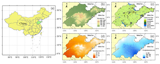
Figure 1.
Overview of the study area. (a) Geographic location, (b) elevation, (c) land cover type, (d) air temperature, and (e) precipitation of the study area.
2.2. Data and Preprocessing
In this study, spatiotemporal sequential data of five meteorological variables (Table 1), namely precipitation (P), vapor pressure deficit (VPD), and wind speed (WS) from TerraClimate [33] and net radiation (RN) and air temperature (TA) from ERA5-Land [34], were employed for predicting regional from TerraClimate. According to Blonquist et al. [35], incorporating net radiative forcing into the correlation features can substantially enhance prediction accuracy. Valipour et al. [36] have also verified, through experimentation, a high correlation between the variables (i.e., P, VPD, WS, RN, and TA) and the ; the values are less than 0.99 for only five provinces in the modified methods. The selected temporal range for the dataset spans from 1980 to 2020, recorded at a monthly scale, and can be accessed through the Google Earth Engine (GEE) platform.

Table 1.
Input features used for the experiment.
The spatial resolutions of the TerraClimate and ERA 5-Land datasets are 4 km × 4 km and 0.1° × 0.1°, respectively. We resampled them using bilinear interpolation to a uniform spatial resolution of 4 km × 4 km and masked them using the study area region. Given the temporal and cyclical characteristics of the data, we partitioned the dataset into training, validation, and test sets based on complete years, with proportions of 70%, 20%, and 10%, respectively. Finally, recognizing the dimensional disparities in the data that hinder direct comparability, we employed the Min-Max normalization method [37] to eliminate differences in dimensional scales among the datasets.
2.3. Method
2.3.1. Flowchart
The workflow of this study is displayed in Figure 2. This work contains four parts: (1) data preprocessing and feature selection; (2) model training, validation, and testing; (3) data prediction; and (4) model evaluation. In the first step, a preprocessing of the dataset was conducted, involving operations such as region cropping, resampling, imputation of missing values, masking, and restoration. The second and third steps involved the training and prediction of using four distinct models (CNN-LSTM, ConvLSTM, SA-ConvLSTM, and MulSA-ConvLSTM). Model weights were obtained through training on the training dataset, and model performance was assessed and compared using both validation and test datasets. The final step involved an experimental evaluation of the trained models using the test dataset to select the optimal model.
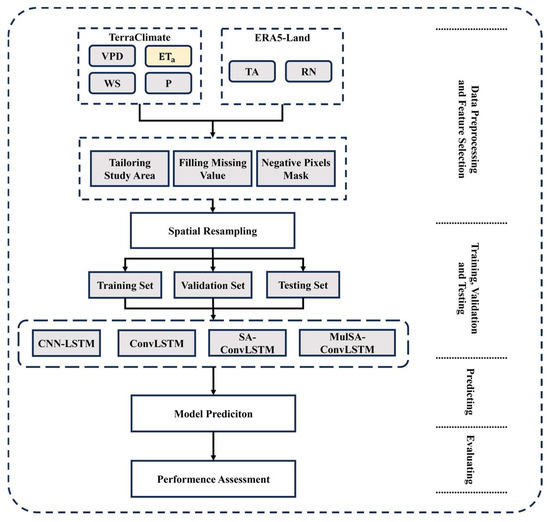
Figure 2.
The flowchart of prediction in this research.
2.3.2. CNN-LSTM
The CNN-LSTM model predicts image sequences in a stacked manner, where the layers of a CNN [38,39] and LSTM [40,41,42] are interleaved. This model employs a CNN’s convolutional operations for feature extraction to capture local features and spatial information [43,44], while the LSTM layer is dedicated to handling time-series prediction [45]. Experiments at the regional scale revealed that LSTM, when using fully connected structures for feature extraction directly, may retain a significant amount of redundant information. By adding convolutional layers before the LSTM layers, the model can more effectively extract spatially correlated information from the feature variables. The convolutional layers utilize convolutional kernel structures and feature matrices for computations, thereby expediting the convergence process of the model. We opted for the CNN-LSTM model to fully leverage the advantages of both CNN and LSTM within a unified framework, using four CNN layers and four LSTM layers, considering the temporal correlations in the data. Specifically, after continuous testing, the convolutional kernels are set to 3 × 3. The sequence length is set to 12 months, as this corresponds to a climate change cycle of approximately 12 months; i.e., 1 month in the future is predicted based on data from the past 12 months.
2.3.3. ConvLSTM
The ConvLSTM [46,47], a derived form of LSTM, extracts feature information through convolutional operations, effectively addressing the intricate relationships between time and space, demonstrating performance in predicting at both the site and regional scales. CNN-LSTM is a simple superposition of CNN and LSTM layers. Different from the CNN-LSTM model, the ConvLSTM model changes the feature extraction method of the LSTM model from fully connected structures to convolutional structures. This architecture, initially proposed by Shi et al. [48], has demonstrated significant effectiveness in tasks involving regional-scale predictions. In contrast to LSTM, which utilizes fully connected structures for input-to-state and state-to-state transitions, ConvLSTM employs a convolutional structure focused on feature extraction. This addresses the issue of spatial redundancy arising from excessive information extraction in LSTM, facilitating the more efficient capturing of spatial dependencies by the model [31]. In this study, the adopted ConvLSTM model is constructed through the stacking of four ConvLSTM layers. Additionally, to enhance learning rate performance, the ReduceLROnPlateau [49] strategy is introduced. ReduceLROnPlateau dynamically adjusts the learning rate based on the model’s training loss while ensuring that the validation loss no longer decreases, thereby improving the model’s convergence during training.
2.3.4. SA-ConvLSTM
The SA-ConvLSTM model [32,50] introduces a SAM with the memory units (Ms) onto the ConvLSTM framework, incorporating the advantages of the SAM module to more effectively capture complex relationships and long-term dependencies within the current spatial context. This augmentation aims to enhance the model’s perception and learning capabilities regarding intricate patterns and relationships. The SAM module combines self-attention mechanisms with memory units to capture long-term spatial dependencies, reinforcing the model’s long-term memory and overcoming challenges faced by ConvLSTM and LSTM models in handling long-term time and space dependencies.
However, the introduction of the SAM module significantly increases the complexity of model training. The intricate network structure and the processing of large-scale regional data pose challenges to limited hardware resources. To address these issues, a block-based training method is employed in this study. During training, large-scale regional data are segmented into smaller-scale regional data. This process involves expanding the channel dimension by n × n times (where n is the number of blocks) and reducing the data size dimension to 1/n × 1/n times. In the final prediction phase, the output images are integrated to the original image size, effectively reducing the spatial complexity during model training. All other models implement a similar block-based training method to ensure fairness in training the models. In this study, the SA-ConvLSTM model adopts a Seq2Seq structure as depicted in Figure 3, stacking four layers of SA-ConvLSTM, with experimental strategies similar to ConvLSTM, including four self-attention nodes and 3 × 3 convolutional kernels. Specifically, after continuous testing, blocks are set to 4. The sequence length is set to 12 months, as this corresponds to a climate change cycle of approximately 12 months; i.e., 1 month in the future is predicted based on data from the past 12 months.
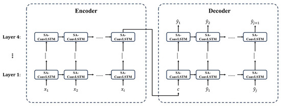
Figure 3.
The SA-ConvLSTM model is employed with the Seq2seq architecture. Arrows delineate the paths for the transmission of feature information. ‘Layer’ signifies the number of layers within the SA-ConvLSTM. Here, represents the i-th input of the model, while denotes the j-th output sequence generated by the model.
2.3.5. MulSA-ConvLSTM
In the framework of SA-ConvLSTM, we conducted in-depth internal structural improvements resulting in MulSA-ConvLSTM. To underscore the remarkable performance of convolutional networks in feature extraction, we introduced a pyramidally multi-scale feature extraction method, namely Pyramidally Attended Feature Extraction (PAFE) [51,52], aimed at enhancing the model’s ability to extract features accurately and comprehensively, thereby capturing global information. Furthermore, we performed a profound refinement of the SAM within the SA-ConvLSTM model, rebranding it as MulSAM. In optimizing the SAM module, we transformed the parallel self-attention module into a parallel multi-headed self-attention module [53,54,55] to strengthen the model’s ability to capture feature information. This study developed the MulSA-ConvLSTM model (Figure 4) by combining PAFE (Figure 4) and the proposed MulSAM module (Figure 5) to accurately capture the spatial feature information. This modification enables the MulSA-ConvLSTM model to more effectively extract feature information across different scales and dimensions. The MulSA-ConvLSTM model adopts an encoder–decoder structure and applies Seq2Seq technology (Figure 6). The encoder consists of four stacked MulSA-ConvLSTM layers, still utilizing a block-based training method, comprising four self-attention nodes and four sets of modules. Specifically, after continuous testing, blocks are set to 4. The sequence length is set to 12 months, as this corresponds to a climate change cycle of approximately 12 months; i.e., 1 month in the future is predicted based on data from the past 12 months.
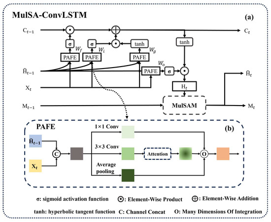
Figure 4.
The network architecture diagram of MulSA-ConvLSTM. The diagram in (a) illustrates the comprehensive cellular structure of the MulSA-ConvLSTM model, while (b) represents the Pyramidally Attended Feature Extraction (PAFE). , , , and represent the weights of the input gate, forget gate, output gate, and update gate, respectively; and represent the candidate states of the input gate and output gate; represents the input at time t; represents the input state at time t − 1; represents the output at time t; and . represent the memory state at time t−1 and t, respectively.
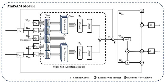
Figure 5.
The internal MulSAM module within the MulSA-ConvLSTM model employs the multi-headed self-attention mechanism, incorporating a multi-headed self-attention module.
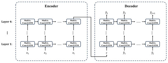
Figure 6.
The MulSA-ConvLSTM model is employed with the Seq2seq architecture. Arrows delineate the paths for the transmission of feature information. ‘Layer’ signifies the number of layers within the MulSA-ConvLSTM. Here, represents the i-th input of the model, while denotes the j-th output sequence generated by the model.
- Pyramidally Attended Feature Extraction (PAFE)
PAFE represents an effective approach in deep learning for integrating information across different scales. This method constructs a pyramid structure to extract features from various scales, aiming to obtain a more comprehensive and rich feature representation. It employs various convolutional kernels with distinct receptive fields or sizes and conducts feature extraction at various levels of the network to extract multi-scale information from input data. This multi-scale feature representation aids in capturing the spatial hierarchy and contextual information of the input data comprehensively, thereby enhancing the model’s performance in handling complex tasks. In this study, PAFE has been successfully applied to the MulSA-ConvLSTM model, effectively capturing the changing trends in . As illustrated in Figure 4, three channels are utilized for feature extraction and integration: one channel employs a 1 × 1 convolutional kernel, another channel uses a 3 × 3 convolutional kernel, and the final channel utilizes average pooling. In the 3 × 3 convolutional kernel channel, an attention mechanism is introduced for feature extraction. This method, by integrating feature information at different spatial scales, enables the model to adapt better to multi-scale variations in the data, resulting in improved performance in extreme predictions and greater sensitivity to climate change.
- b.
- MulSAM module
The proposed MulSAM module, as illustrated in Figure 5, builds upon the SAM module with significant improvements, primarily by incorporating the multi-headed self-attention module from the Transformer model [53] to enhance the SAM module’s spatial feature capture capabilities. By using multiple independent attentional heads, the attentional weights are computed separately, and their results are weighted and summed. The outputs of multiple self-attention mechanisms are then passed through a parameter matrix to obtain a new output. The single-head parallel self-attention mechanism in the SAM module is modified to a parallel multi-headed self-attention module as illustrated in Figure 5, allowing the MulSA-ConvLSTM model to focus on information from different subspaces at different positions, capturing spatial correlations in the data more comprehensively and flexibly. This enhancement enables the multi-headed self-attention module to capture a more diverse set of feature information.
2.3.6. Model Performance Metrics
In order to assess the performance of the model, five metrics are employed, namely the Pearson correlation coefficient (R) [56], root mean square error (RMSE), mean absolute error (MAE), correlation coefficient () [57], and bias. The computation formulas are as follows:
In this context, and denote the ith observed and predicted values, respectively, where N represents the sample size of the evaluation dataset. and denote the mean of observed and predicted values, respectively. The value of R and approaching 1 indicates that the predicted values are close to the observed values. Bias reflects the disparity between predicted and observed values. RMSE and MAE are commonly used evaluation metrics for time-series forecasting, with lower values indicating superior predictive performance of the model.
3. Results
3.1. Spatiotemporal Evaluation of Regional-Scale Prediction Models
The performance of the four models for predicting regional-scale is illustrated in Figure 7, encompassing their RMSE, MAE, R, and bias during prediction within the study area. The MulSA-ConvLSTM has the best performance compared to other contrast models.
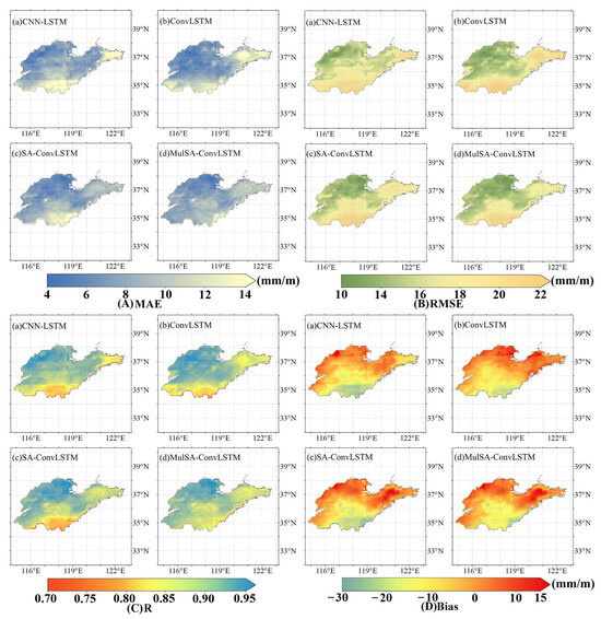
Figure 7.
The four models exhibit distributional maps of the (A) mean absolute error (MAE), (B) root mean square error (RMSE), (C) correlation coefficient (R), and (D) bias in predicting for the testing set spanning the years 2016 to 2020. (a) CNN-LSTM; (b) ConvLSTM; (c) SA-ConvLSTM; (d) MulSA-ConvLSTM. The numbers in the legend represent the numerical values for each of the assessment indicators, with the corresponding units to the right of the legend (mm/m: mm per month).
The distribution of MAE and RMSE, as depicted in Figure 7A,B, reveals that all four models exhibit relatively lower MAE and RMSE values in the northern of the study area than in the southern regions. Particularly, the consistently lowest MAE and RMSE values are exhibited by the MulSA-ConvLSTM model across the entire study area. In contrast, CNN-LSTM, ConvLSTM, and SA-ConvLSTM exhibit varying degrees of high MAE and RMSE values in regions with high elevation differences. Specifically, the ConvLSTM model exhibits high MAE values and RMSE values in the eastern coastal regions with high elevation differences, higher than 12 mm/m and 18 mm/m in the region to the east of 120°E, respectively, while the SA-ConvLSTM model presents high MAE and RMSE values when predicting in the southern regions with high elevation differences, higher than 12 mm/m and 18 mm/m in the region to the south of 35.5°N, respectively. Noteworthily, the CNN-LSTM model shows high MAE and RMSE values in both the eastern coastal and southern regions with high elevation differences, higher than 12 mm/m and 18 mm/m in the regions both to the east of 120°E and the south of 35.5°N, respectively. The ConvLSTM model demonstrates lower MAE and RMSE values when predicting for the central regions with high elevation differences, lower than 8 mm/m and 15 mm/m in the regions both to the west of 120°E and the north of 35.5°N, respectively. Due to the relatively flat terrain in the northern regions, devoid of topographical influences, the four models exhibited distinct trends in MAE and RMSE values when confronted with variations between coastal and inland areas. The MAE and RMSE values obtained by SA-ConvLSTM and MulSA-ConvLSTM in predicting coastal regions’ are significantly lower than those for inland regions, lower than 10 mm/m and 17 mm/m in the regions both to the east of 120°E and the north of 36.5°N, respectively, while the MAE and RMSE values obtained by CNN-LSTM and ConvLSTM have no significant differences.
According to the data illustrated in Figure 7C, the correlation coefficients (R) of the four models within the study area exhibit a gradual increase from south to north, displaying higher correlations of predicting values in regions with low elevation differences than in ones with high elevation differences. These models demonstrate relatively good and consistent performance when predicting in the flat topography regions. While CNN-LSTM and ConvLSTM show a decreasing trend in R values when predicting values for regions with high elevation differences in the eastern coastal area, conversely, SA-ConvLSTM and MulSA-ConvLSTM maintain relatively higher correlations when predicting in these regions. Both CNN-LSTM and ConvLSTM exhibit lower sensitivity to variations in northern inland and coastal regions, resulting in no significant differences in R values between predicting for these two areas. However, in the prediction of , the SA-ConvLSTM and MulSA-ConvLSTM models showcase notably higher correlation coefficients in coastal regions compared to inland regions.
Figure 7D shows the bias values of all models in predicting regional-scale . Consistent and robust performances are presented across the four models in predicting the of northern regions with flat topography. However, when confronted with areas with high elevation differences, these models exhibit a tendency to either overestimate or underestimate . Overall, these models tend to underestimate in the southern regions with high elevation differences, with bias values lower than −10 mm/m in the regions both to the east of 117°E and the south of 35.5°N. Both CNN-LSTM and ConvLSTM models show a trend of underestimation in prediction across the entire study area, with the degree of underestimation gradually increasing with elevation differences. In contrast, the SA-ConvLSTM and MulSA-ConvLSTM models demonstrate a trend of overestimation in prediction for regions with high elevation differences along the eastern coast. Notably, for regions with high elevation differences, the MulSA-ConvLSTM model exhibits the smallest prediction bias compared to other models, lower than −15 mm/m in the regions both to the east of 117°E and the south of 35.5°N, while CNN-LSTM performs the least favorably, lower than −20 mm/m in the regions both to the east of 117°E and the south of 35.5°N. Unlike the other models, ConvLSTM shows a trend of overestimation in prediction across the northern coastal regions, higher than 5 mm/m in the regions both to the east of 118°E and the north of 37.5°N. The other models all show varying degrees of underestimation in prediction across the northern regions.
The introduction of the SAM module significantly enhances the performance of the SA-ConvLSTM model, and the MulSA-ConvLSTM model further improves predictive capabilities through the incorporation of the multi-headed self-attention modules. In a comprehensive comparison of the bias among the four models, the MulSA-ConvLSTM model emerges as the most effective in terms of overall performance.
Table 2 shows the RMSE values of four models for each land cover type. From Figure 1c, it can be seen that the study area is mainly characterized by croplands. The RMSE values for shrublands, forests, and barren land are lower than those for other land cover types, and urban land has the highest RMSE values. Figure 8 shows that the RMSE values varied with elevation. From Figure 1b, it can be seen that the areas below 100 m elevation are mainly located in the northern part of the study area and the southern and marginal regions. The area below 100 m elevation in the north is flat and has a lower average RMSE value. However, due to the complex terrain and concentration of urban land in the southern part of the area below 100 m elevation, the average RMSE values of the area below 100 m elevation show different degrees of increase. All models presented higher RMSE values in the range of 100 to 200 m elevation above mean sea level, followed by a gradual decrease in RMSE values with increasing elevations. This is because the area between 100 and 200 m elevation above mean sea level is located on the south and east coast of the study area, which has complex terrain with significant elevation changes and concentrations of urban land. However, above 200 m elevation, ConvLSTM shows lower RMSE values in the study area, and there is a concentration of shrublands and forests in this area. Additionally, CNN-LSTM shows a more moderate change in RMSE values throughout the study area. Based on the analysis, it looks like changes in elevation magnitude have a bigger impact on the model’s accuracy than increases in elevation, and areas with complex terrain tend to have lower model accuracy compared to those with flat terrain. Also, areas with urban land tend to have lower model accuracy compared to those with shrublands and forests.

Table 2.
The RMSE values of four models for each land cover type.
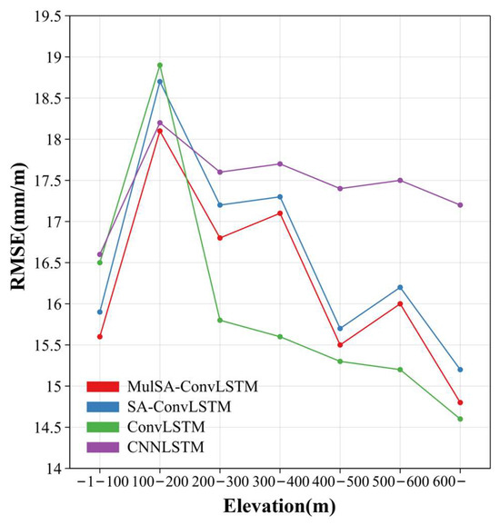
Figure 8.
The plot of elevation versus error. Trends in RMSE with elevation.
Table 3 provides data illustrating that the MulSA-ConvLSTM model exhibits the smallest RMSE and MAE while achieving the maximum R value (R = 0.908, RMSE = 16.6 mm/m, MAE = 8.6 mm/m) in predicting . MulSA-ConvLSTM demonstrates improvements of 2.9%, 4.4%, and 5.4% in R compared to SA-ConvLSTM, ConvLSTM, and CNN-LSTM, respectively. Correspondingly, RMSE decreases by 1.8%, 3.0%, and 4.8%, and MAE decreases by 2.2%, 4.5%, and 8.9%. Furthermore, when comparing the biases among the four models, it is evident that MulSA-ConvLSTM exhibits the smallest bias, demonstrating the most stable performance in predicting . Therefore, MulSA-ConvLSTM is considered the optimal model for prediction.

Table 3.
Comparative evaluation of the prediction results of four deep learning models.
According to the above-mentioned analysis, we select the SA-ConvLSTM model and our developed MulSA-ConvLSTM model, with better prediction accuracy than the other two, to draw the time-series prediction results, shown in Figure 9. The predictions by SA-ConvLSTM and MulSA-ConvLSTM exhibit a trend of fluctuation around the actual observed values. It is noteworthy that, particularly in months with relatively extreme variations in (such as January 2018, January 2019, and December 2019), the predictions from MulSA-ConvLSTM are closer to the observed values than those from SA-ConvLSTM. In comparison to SA-ConvLSTM, MulSA-ConvLSTM captures the trends in more effectively, bringing its predictions closer to the actual variations in . This implies that MulSA-ConvLSTM exhibits enhanced performance in predicting under extreme conditions, providing robust support for the model’s resilience and accuracy.
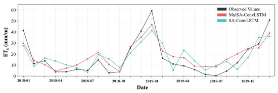
Figure 9.
The temporal variations in the monthly mean values of from 2018 to 2020 were examined, and a comparative analysis was conducted between two predictive models. The observed values of are represented by the black line, while the predictions from the MulSA-ConvLSTM model are depicted in red, and those from the SA-ConvLSTM model are represented by the green line.
3.2. Performance Evaluation of Regional-Scale Prediction Models
The loss function plots during training and validation epochs for the four models are shown in Figure 10. MulSA-ConvLSTM exhibits the lowest training and validation losses, indicative of its superior performance in predicting . Concurrently, due to its simplest model architecture, the CNN-LSTM model demonstrates the fastest convergence speed during the training process. ConvLSTM, SA-ConvLSTM, and MulSA-ConvLSTM all exhibit signs of convergence around 50 epochs. The presence of self-attention modules in SA-ConvLSTM and MulSA-ConvLSTM facilitates a more effective capture of feature change trends during the training process compared to ConvLSTM. Therefore, SA-ConvLSTM and MulSA-ConvLSTM manifest an enhanced propensity for expedited convergence in contrast to ConvLSTM. During the training process, the validation loss values for these four models consistently remained higher than the training loss values, indicating that the employed models demonstrated neither overfitting nor underfitting.
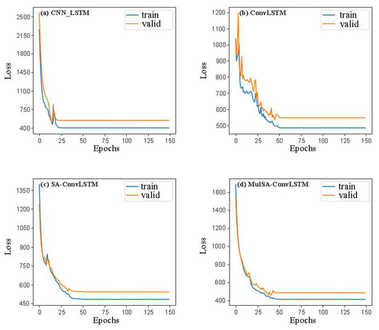
Figure 10.
Loss function plots for the four models predicting . (a) CNN-LSTM; (b) ConvLSTM; (c) SA-ConvLSTM; (d) MulSA-ConvLSTM.
Compared to SA-ConvLSTM, the addition of the SAM in ConvLSTM enhances the model’s capability to capture and retain long-term spatial information, resulting in a 3% improvement in prediction accuracy. MulSA-ConvLSTM further reinforces the model’s capacity to capture long-term spatial information and extract feature information. However, the increased complexity of the model leads to a rise in the number of parameters and training duration. According to Table 4, in comparison to SA-ConvLSTM and ConvLSTM, MulSA-ConvLSTM experiences an increment of 0.8 million (M) and 1.3 million parameters, accompanied by an additional 3 s and 6 s per training iteration, respectively. The LSTM layer within the CNN-LSTM model adopts fully connected layers for feature extraction, resulting in a bigger volume of used parameters than the other compared models, reaching 430.2 M. Despite having the highest parameter count, CNN-LSTM requires the shortest training time. In summary, considering the comprehensive evaluation based on training time, parameter count, and accuracy, the MulSA-ConvLSTM model is deemed the most effective among the four models for predicting .

Table 4.
Efficiency comparison of four deep learning models.
4. Discussion
4.1. Impact of Environmental Factors on Prediction Accuracy
The experimental results indicate that the model has deviations under complex terrain and climatic conditions. On the one hand, when facing regions with different climates, both SA-ConvLSTM and MulSA-ConvLSTM exhibit noticeable sensitivity. Specifically, the northern part of the study area exhibits a relatively flat topography, with its eastern boundary being adjacent to the coastline. As shown in Figure 7, there is a significant difference in prediction accuracy when predicting in coastal and inland areas. The prediction accuracy in coastal areas outperforms that of inland areas when the interference of topography is lost. In contrast, CNN-LSTM and ConvLSTM show low sensitivity in prediction accuracy when predicting in the northern sector of the study area.
On the other hand, the accuracy of the model in predicting changes with elevation differences and land cover type. The model’s prediction accuracy decreases as regional elevation differences and urban area increase. Also, from Figure 1d,e and Figure 6, it can be seen that the accuracy of the model in predicting changes with air temperature and precipitation. This phenomenon is more evident when comparing the prediction accuracy of in the southern and northern parts of the study area, as illustrated in Figure 7. The accuracy of the model in predicting is relatively high in the northern part of the region, with R values higher than 0.88 in the regions both to the west of 120°E and the north of 36.5°N, because of the flat terrain, low air temperature, and precipitation, whereas in the southern part of the region with many mountain ranges, the complex terrain, high air temperature, high precipitation, and concentration of urban area result in a generally low accuracy of the model in predicting , with R values lower than 0.87 in the regions both to the east of 117°E and the south of 35.5°N. Despite the eastern part of the Shandong Peninsula being located in a coastal area, the numerous mountains and complex terrain in this region pose challenges for accurately predicting . It is noted that the TerraClimate data used in this study are interpolations of several datasets, taking into account orography, at a relatively high resolution. TerraClimate data are based on WorldClim data [58], which in turn use CRU data [59]. There are regions where the observations are very sparse, and the interpolations, especially of precipitation [60], are quite different from other observations. Furthermore, the interpolation method used fails to maintain coherence between the various variables as they are interpolated independently. Errors from the interpolation process may result in neural models learning patterns that do not exist in regions with complex orography.
Both SA-ConvLSTM and MulSA-ConvLSTM are equipped with self-attention mechanism modules, aiding in better capturing feature information when facing climate and altitude variations. Particularly, MulSA-ConvLSTM, through the effective utilization of the multi-headed self-attention module and the PAFE method in the MulSAM module, extracts feature information and spatial dependencies across different dimensions, angles, and scales. Consequently, MulSA-ConvLSTM demonstrates robust stability in complex natural ecological environments.
4.2. Impact of Pixels’ Location on Prediction Accuracy
The accuracy of the models used in this study is affected when the feature variables fail to provide sufficient pixel information. This is because the models employ the CNN module for feature extraction, which comprehensively considers pixel data around specified pixels in the grid dataset. Cropping boundary pixels is the way to eliminate outliers when predicting regional scale . Since is only meaningful to terrestrial regions, there is no available for marine areas. The Shandong Peninsula is located in the coastal zone, which means that there is no information available beyond the coastline. During feature fitting, missing values of in the extracted marine regions can negatively affect the accuracy of predictions near the study area boundaries. As the coastline is situated at the border of the study area, it is not possible to eliminate the adverse effects of outliers by cropping.
A block-based training method was adopted to address the computational challenges posed by large-scale data during model training. The accuracy of predicting features near the boundaries is lower due to the limited pixel information in those areas. When predicting pixels in the central region of the study area in a block-based approach without cropping boundary pixels, the model’s accuracy may decrease due to insufficient boundary information. Although the use of the spatial correlation of the feature variables can improve the prediction of regional-scale , inaccurate predictions may result due to insufficient information near the boundary pixels.
4.3. Sensitivity Analysis of Features
The large-scale and accurate predictions of contribute to a more precise assessment and forecasting of hydrological and ecosystem processes, holding significant practical applications in fields such as agriculture, ecology, and meteorology. In the realm of handling intricate data, deep learning exhibits significant advantages, enabling the automatic extraction of advanced feature representations from raw datasets. To further research the interrelations between and various variables, we conducted a sensitivity analysis of feature variables in the study area using the MulSA-ConvLSTM model. Firstly, a sensitivity analysis of individual features was performed, systematically inputting each feature variable separately into the model for training and predicting , thus observing the impact of each variable on the prediction accuracy of . Secondly, a sensitivity analysis was conducted for missing features, systematically excluding one feature variable at a time and employing the remaining feature variables for training across all models, thereby observing changes in the prediction accuracy of under the absence of different variables. Finally, the method proposed by Zhao et al. [61] was utilized to conduct a sensitivity analysis for increasing feature values. To achieve this, one variable was increased in 10% increments as a disturbance value while the remaining features were kept unchanged. The disturbance range was between 0 and 90%, and the resulting effect on prediction accuracy with the increase in the magnitude of the disturbance was observed.
Deep learning possesses a notable advantage in handling complex data, as it autonomously learns advanced feature representations from raw datasets. The experimental results in Table 5 indicate that, when using the meteorological element WS in isolation, the correlation coefficient (R) reaches its highest value at 0.769. Conversely, employing RN and TA individually yields the lowest R values, specifically 0.645 and 0.611, respectively. The training outcomes of the model reveal varying degrees of reduction in prediction accuracy due to the absence of different feature variables. Notably, as shown in Table 6, the omission of RN significantly impacts prediction accuracy, with an R of only 0.733. Compared to the absence of RN and WS, the absence of VPD and WS has a relatively lesser effect on prediction accuracy, with correlation coefficients of 0.815 and 0.744, respectively. The influence of P’s absence on prediction accuracy is minimal, with an R of 0.839. The optimal performance observed when considering all five features as input data confirms the rationality of the chosen input data. Notably, Figure 11 assays show that alterations in WS, P, and RN produce the most significant impact on prediction, particularly when increased to 50% at maximum.

Table 5.
Sensitivity analysis of one feature. Sensitivity analyses were conducted on individual features. The abbreviations “RN”, “TA”, “WS”, “VPD”, and “P” are used to represent the input variables.

Table 6.
Sensitivity analysis regarding the absence of one variable. Sensitivity analyses were conducted after removing a feature, using the remaining features as input variables. The abbreviations “RN”, “TA”, “WS”, “VPD”, and “P” are used to represent the removed features.
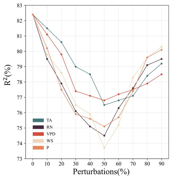
Figure 11.
Sensitivity analyses for adding perturbation values. “RN”, “TA”, “WS”, “VPD”, and “P” denote the characteristic variables with added perturbation values.
During the model training process, the pivotal role of RN as an input feature highlights its significant impact on the process. By prioritizing RN as a primary input, we anticipate capturing dynamic variations in evapotranspiration more accurately, thereby enhancing the model’s adaptability to environmental changes. Consequently, incorporating RN as an input feature in the prediction model holds the potential to improve model robustness and predictive performance [62]. VPD and TA jointly determine the relative humidity in the air [63], mutually influencing variations in . VPD represents the air’s moisture dryness and plays an indispensable role in regulating plant transpiration, moisture transport, and ecosystem water cycling. WS and P also play crucial roles in prediction; in relatively humid regions, wind speed has a significant impact on , whereas in relatively dry areas, ’s dynamic changes closely follow precipitation variations, rendering wind speed negligible [64,65]. Observing the patterns of variation among features contributes to a deeper understanding of the interplay of various meteorological factors under the backdrop of global warming.
This analytical approach allows for a systematic evaluation of the contribution of each feature variable to model predictions and an examination of the impact of missing features on predictive performance. By comparing the performance of the model under single and multiple feature scenarios, a comprehensive understanding of each variable’s role in the MulSA-ConvLSTM model is achieved, providing valuable insights for the application of deep learning in hydrology and ecology.
5. Conclusions
To improve the regional prediction of , a MulSA-ConvLSTM model was developed in this study. The MulSA-ConvLSTM model and three other models (i.e., CNN-LSTM, ConvLSTM, SA-ConvLSTM) were used to predict large-scale regional in the Shandong Peninsula. The model performances were evaluated using RMSE, MAE, R, and bias metrics. The main conclusions include the following:
- The introduction of PAFE proves to be more efficient in extracting local features and the spatial information of feature variables. Additionally, the results indicate that incorporating a multi-headed self-attention module in the MulSAM module enhances the model’s ability to comprehensively understand the input data features. This improvement allows the model to better adapt to feature relationships at different scales and angles, thereby enhancing its representational capacity and effectively adapting to complex environmental changes.
- Among the four models, the MulSA-ConvLSTM model exhibited superior predictive performance for , with SA-ConvLSTM slightly outperforming CNN-LSTM and ConvLSTM. Specifically, the experimental results of MulSA-ConvLSTM (R = 0.908) showed a 2% improvement compared to SA-ConvLSTM (R = 0.882). As the elevation difference of the study area increases, the prediction accuracy of all four models generally exhibits a declining trend.
- MulSA-ConvLSTM demonstrates higher precision in predicting than the three other models in regions with high elevation differences. Moreover, MulSA-ConvLSTM and SA-ConvLSTM show heightened sensitivity to characteristic changes in coastal areas, showcasing superior performance in prediction experiments.
Author Contributions
Methodology, X.Z.; Software, X.Z.; Validation, X.Z.; Formal analysis, X.Z.; Investigation, X.Z.; Data curation, X.Z.; Writing—original draft, X.Z.; Writing—review & editing, S.Z., J.Z., S.Y., J.H., X.M. and Y.B.; Visualization, X.Z.; Supervision, S.Z., J.Z., S.Y. and Y.B.; Funding acquisition, S.Z., J.Z., S.Y. and Y.B. All authors have read and agreed to the published version of the manuscript.
Funding
This work was supported by the Excellent Young Scientist Fund of Natural Science Foundation of Hebei Province (Grant No. D2023205012), the National Natural Science Foundation of China (42101382 and 42201407) and the Shandong Provincial Natural Science Foundation (ZR2020QD016 and ZR2022QD120).
Data Availability Statement
The data presented in this study are available in Muñoz Sabater, J., (2019): ERA5-Land monthly averaged data from 1981 to present. Copernicus Climate Change Service (C3S) Climate Data Store (CDS) at doi:10.24381/cds.68d2bb30; Abatzoglou, J.T., S.Z. Dobrowski, S.A. Parks, K.C. Hegewisch, 2018, Terraclimate, a high-resolution global dataset of monthly climate and climatic water balance from 1958–2015, Scientific Data 5:170191 at doi:10.1038/sdata.2017.191.
Conflicts of Interest
The authors declare no conflict of interest.
References
- Bharati, L.; Rodgers, C.; Erdenberger, T.; Plotnikova, M.; Shumilov, S.; Vlek, P.; Martin, N. Integration of economic and hydrologic models: Exploring conjunctive irrigation water use strategies in the Volta Basin. Agric. Water Manag. 2008, 95, 925–936. [Google Scholar] [CrossRef]
- Yang, Y.; Yang, Y.; Liu, D.L.; Nordblom, T.; Wu, B.; Yan, N. Regional water balance based on remotely sensed evapotranspiration and irrigation: An assessment of the Haihe Plain, China. Remote Sens. 2014, 6, 2514–2533. [Google Scholar] [CrossRef]
- Paul, M.; Rajib, A.; Negahban-Azar, M.; Shirmohammadi, A.; Srivastava, P. Improved agricultural Water management in data-scarce semi-arid watersheds: Value of integrating remotely sensed leaf area index in hydrological modeling. Sci. Total Environ. 2021, 791, 148177. [Google Scholar] [CrossRef] [PubMed]
- Wanniarachchi, S.; Sarukkalige, R. A review on evapotranspiration estimation in agricultural water management: Past, present, and future. Hydrology 2022, 9, 123. [Google Scholar] [CrossRef]
- Jackson, R.B.; Carpenter, S.R.; Dahm, C.N.; McKnight, D.M.; Naiman, R.J.; Postel, S.L.; Running, S.W. Water in a changing world. Ecol. Appl. 2001, 11, 1027–1045. [Google Scholar] [CrossRef]
- Devia, G.K.; Ganasri, B.P.; Dwarakish, G.S. A review on hydrological models. Aquat. Procedia 2015, 4, 1001–1007. [Google Scholar] [CrossRef]
- Herman, M.R.; Nejadhashemi, A.P.; Abouali, M.; Hernandez-Suarez, J.S.; Daneshvar, F.; Zhang, Z.; Anderson, M.C.; Sadeghi, A.M.; Hain, C.R.; Sharifi, A. Evaluating the role of evapotranspiration remote sensing data in improving hydrological modeling predictability. J. Hydrol. 2018, 556, 39–49. [Google Scholar] [CrossRef]
- Calera, A.; Campos, I.; Osann, A.; D’Urso, G.; Menenti, M. Remote sensing for crop water management: From ET modelling to services for the end users. Sensors 2017, 17, 1104. [Google Scholar] [CrossRef] [PubMed]
- Anapalli, S.S.; Fisher, D.K.; Reddy, K.N.; Rajan, N.; Pinnamaneni, S.R. Modeling evapotranspiration for irrigation water management in a humid climate. Agric. Water Manag. 2019, 225, 105731. [Google Scholar] [CrossRef]
- Gorguner, M.; Kavvas, M.L. Modeling impacts of future climate change on reservoir storages and irrigation water demands in a Mediterranean basin. Sci. Total Environ. 2020, 748, 141246. [Google Scholar] [CrossRef] [PubMed]
- Bastiaanssen, W.G.M.; Noordman, E.J.M.; Pelgrum, H.; Davids, G.; Thoreson, B.P.; Allen, R.G. SEBAL model with remotely sensed data to improve water-resources management under actual field conditions. J. Irrig. Drain. Eng. 2005, 131, 85–93. [Google Scholar] [CrossRef]
- Cao, G.; Han, D.; Song, X. Evaluating actual evapotranspiration and impacts of groundwater storage change in the North China Plain. Hydrol. Process. 2014, 28, 1797–1808. [Google Scholar] [CrossRef]
- Sang, J.; Hou, B.; Wang, H.; Ding, X. Prediction of water resources change trend in the Three Gorges Reservoir Area under future climate change. J. Hydrol. 2023, 617, 128881. [Google Scholar] [CrossRef]
- Farooque, A.A.; Afzaal, H.; Abbas, F.; Bos, M.; Maqsood, J.; Wang, X.; Hussain, N. Forecasting daily evapotranspiration using artificial neural networks for sustainable irrigation scheduling. Irrig. Sci. 2022, 40, 55–69. [Google Scholar] [CrossRef]
- Ferreira, L.B.; da Cunha, F.F.; Fernandes Filho, E.I. Exploring machine learning and multi-task learning to estimate meteorological data and reference evapotranspiration across Brazil. Agric. Water Manag. 2022, 259, 107281. [Google Scholar] [CrossRef]
- Hashemi, M.; Sepaskhah, A.R. Evaluation of artificial neural network and Penman–Monteith equation for the prediction of barley standard evapotranspiration in a semi-arid region. Theor. Appl. Climatol. 2020, 139, 275–285. [Google Scholar] [CrossRef]
- Roy, D.K. Long short-term memory networks to predict one-step ahead reference evapotranspiration in a subtropical climatic zone. Environ. Process. 2021, 8, 911–941. [Google Scholar] [CrossRef]
- Chen, R.; Wang, X.; Zhang, W.; Zhu, X.; Li, A.; Yang, C. A hybrid CNN-LSTM model for typhoon formation forecasting. GeoInformatica 2019, 23, 375–396. [Google Scholar] [CrossRef]
- Cai, H.; Shi, H.; Liu, S.; Babovic, V. Impacts of regional characteristics on improving the accuracy of groundwater level prediction using machine learning: The case of central eastern continental United States. J. Hydrol. Reg. Stud. 2021, 37, 100930. [Google Scholar] [CrossRef]
- Granata, F. Evapotranspiration evaluation models based on machine learning algorithms—A comparative study. Agric. Water Manag. 2019, 217, 303–315. [Google Scholar] [CrossRef]
- Ball, J.E.; Anderson, D.T.; Chan, C.S. Comprehensive survey of deep learning in remote sensing: Theories, tools, and challenges for the community. J. Appl. Remote Sens. 2017, 11, 042609. [Google Scholar] [CrossRef]
- Lary, D.J.; Alavi, A.H.; Gandomi, A.H.; Walker, A.L. Machine learning in geosciences and remote sensing. Geosci. Front. 2016, 7, 3–10. [Google Scholar] [CrossRef]
- e Lucas, P.D.O.; Alves, M.A.; e Silva, P.C.D.L.; Guimaraes, F.G. Reference evapotranspiration time series forecasting with ensemble of convolutional neural networks. Comput. Electron. Agric. 2020, 177, 105700. [Google Scholar] [CrossRef]
- Ferreira, L.B.; da Cunha, F.F. New approach to estimate daily reference evapotranspiration based on hourly temperature and relative humidity using machine learning and deep learning. Agric. Water Manag. 2020, 234, 106113. [Google Scholar] [CrossRef]
- Ferreira, L.B.; da Cunha, F.F. Multi-step ahead forecasting of daily reference evapotranspiration using deep learning. Comput. Electron. Agric. 2020, 178, 105728. [Google Scholar] [CrossRef]
- Nagappan, M.; Gopalakrishnan, V.; Alagappan, M. Prediction of reference evapotranspiration for irrigation scheduling using machine learning. Hydrol. Sci. J. 2020, 65, 2669–2677. [Google Scholar] [CrossRef]
- Sharma, G.; Singh, A.; Jain, S. Hybrid deep learning techniques for estimation of daily crop evapotranspiration using limited climate data. Comput. Electron. Agric. 2022, 202, 107338. [Google Scholar] [CrossRef]
- Alibabaei, K.; Gaspar, P.D.; Lima, T.M. Modeling soil water content and reference evapotranspiration from climate data using deep learning method. Appl. Sci. 2021, 11, 5029. [Google Scholar] [CrossRef]
- Dong, J.; Zhu, Y.; Jia, X.; Han, X.; Qiao, J.; Bai, C.; Tang, X. Nation-scale reference evapotranspiration estimation by using deep learning and classical machine learning models in China. J. Hydrol. 2022, 604, 127207. [Google Scholar] [CrossRef]
- Li, Y.; Wang, W.; Wang, G.; Tan, Q. Actual evapotranspiration estimation over the Tuojiang River Basin based on a hybrid CNN-RF model. J. Hydrol. 2022, 610, 127788. [Google Scholar] [CrossRef]
- Babaeian, E.; Paheding, S.; Siddique, N.; Devabhaktuni, V.K.; Tuller, M. Short-and mid-term forecasts of actual evapotranspiration with deep learning. J. Hydrol. 2022, 612, 128078. [Google Scholar] [CrossRef]
- Xiong, T.; He, J.; Wang, H.; Tang, X.; Shi, Z.; Zeng, Q. Contextual Sa-attention convolutional LSTM for precipitation nowcasting: A spatiotemporal sequence forecasting view. IEEE J. Sel. Top. Appl. Earth Obs. Remote Sens. 2021, 14, 12479–12491. [Google Scholar] [CrossRef]
- Abatzoglou, J.T.; Dobrowski, S.Z.; Parks, S.A.; Hegewisch, K.C. TerraClimate, a high-resolution global dataset of monthly climate and climatic water balance from 1958–2015. Sci. Data 2018, 5, 170191. [Google Scholar] [CrossRef] [PubMed]
- Muñoz-Sabater, J.; Dutra, E.; Agustí-Panareda, A.; Albergel, C.; Arduini, G.; Balsamo, G.; Boussetta, S.; Choulga, M.; Harrigan, S.; Hersbach, H.; et al. ERA5-Land: A state-of-the-art global reanalysis dataset for land applications. Earth Syst. Sci. Data 2021, 13, 4349–4383. [Google Scholar] [CrossRef]
- Blonquist, J., Jr.; Allen, R.; Bugbee, B. An evaluation of the net radiation sub-model in the ASCE standardized reference evapotranspiration equation: Implications for evapotranspiration prediction. Agric. Water Manag. 2010, 97, 1026–1038. [Google Scholar] [CrossRef]
- Valipour, M. Importance of solar radiation, temperature, relative humidity, and wind speed for calculation of reference evapotranspiration. Arch. Agron. Soil Sci. 2015, 61, 239–255. [Google Scholar] [CrossRef]
- Patro, S.; Sahu, K.K. Normalization: A preprocessing stage. arXiv 2015, arXiv:1503.06462. [Google Scholar] [CrossRef]
- O’Shea, K.; Nash, R. An introduction to convolutional neural networks. arXiv 2015, arXiv:1511.08458. [Google Scholar]
- Gu, J.; Wang, Z.; Kuen, J.; Ma, L.; Shahroudy, A.; Shuai, B.; Liu, T.; Wang, X.; Wang, G.; Cai, J.; et al. Recent advances in convolutional neural networks. Pattern Recognit. 2018, 77, 354–377. [Google Scholar] [CrossRef]
- Cho, K.; Van Merriënboer, B.; Gulcehre, C.; Bahdanau, D.; Bougares, F.; Schwenk, H.; Bengio, Y. Learning phrase representations using RNN encoder-decoder for statistical machine translation. arXiv 2014, arXiv:1406.1078. [Google Scholar]
- Shewalkar, A.; Nyavanandi, D.; Ludwig, S.A. Performance evaluation of deep neural networks applied to speech recognition: RNN, LSTM and GRU. J. Artif. Intell. Soft Comput. Res. 2019, 9, 235–245. [Google Scholar] [CrossRef]
- Sherstinsky, A. Fundamentals of recurrent neural network (RNN) and long short-term memory (LSTM) network. Phys. D Nonlinear Phenom. 2020, 404, 132306. [Google Scholar] [CrossRef]
- Alzubaidi, L.; Zhang, J.; Humaidi, A.J.; Al-Dujaili, A.; Duan, Y.; Al-Shamma, O.; Santamaría, J.; Fadhel, M.A.; Al-Amidie, M.; Farhan, L. Review of deep learning: Concepts, CNN architectures, challenges, applications, future directions. J. Big Data 2021, 8, 53. [Google Scholar] [CrossRef] [PubMed]
- Kattenborn, T.; Leitloff, J.; Schiefer, F.; Hinz, S. Review on Convolutional Neural Networks (CNN) in vegetation remote sensing. ISPRS J. Photogramm. Remote Sens. 2021, 173, 24–49. [Google Scholar] [CrossRef]
- Yu, Y.; Si, X.; Hu, C.; Zhang, J. A review of recurrent neural networks: LSTM cells and network architectures. Neural Comput. 2019, 31, 1235–1270. [Google Scholar] [CrossRef] [PubMed]
- Kim, S.; Hong, S.; Joh, M.; Song, S.-k. Deeprain: Convlstm network for precipitation prediction using multichannel radar data. arXiv 2017, arXiv:1711.02316. [Google Scholar]
- Moishin, M.; Deo, R.C.; Prasad, R.; Raj, N.; Abdulla, S. Designing deep-based learning flood forecast model with ConvLSTM hybrid algorithm. IEEE Access 2021, 9, 50982–50993. [Google Scholar] [CrossRef]
- Shi, X.; Chen, Z.; Wang, H.; Yeung, D.-Y.; Wong, W.-K.; Woo, W.-C. Convolutional LSTM Network: A Machine Learning Approach for Precipitation Nowcasting. In Advances in Neural Information Processing Systems 28 (NIPS 2015); MIT Press: Cambridge, MA, USA, 2015. [Google Scholar]
- Lewkowycz, A. How to decay your learning rate. arXiv 2021, arXiv:2103.12682. [Google Scholar]
- Lin, Z.; Li, M.; Zheng, Z.; Cheng, Y.; Yuan, C. Self-attention convlstm for spatiotemporal prediction. In Proceedings of the AAAI Conference on Artificial Intelligence, New York, NY, USA, 7–12 February 2020; AAAI Press: Washington, DC, USA, 2020; Volume 34, pp. 11531–11538. [Google Scholar]
- He, K.; Zhang, X.; Ren, S.; Sun, J. Spatial pyramid pooling in deep convolutional networks for visual recognition. IEEE Trans. Pattern Anal. Mach. Intell. 2015, 37, 1904–1916. [Google Scholar] [CrossRef] [PubMed]
- Zhao, X.; Zhang, L.; Pang, Y.; Lu, H.; Zhang, L. A Single Stream Network for Robust and Real-Time RGB-D Salient Object Detection. In Computer Vision—ECCV 2020; Springer: Cham, Switzerland, 2020; pp. 646–662. [Google Scholar]
- Vaswani, A.; Shazeer, N.; Parmar, N.; Uszkoreit, J.; Jones, L.; Gomez, A.N.; Kaiser, Ł.; Polosukhin, I. Attention Is All You Need. In Advances in Neural Information Processing Systems 30 (NIPS 2017); MIT Press: Cambridge, MA, USA, 2017. [Google Scholar]
- Voita, E.; Talbot, D.; Moiseev, F.; Sennrich, R.; Titov, I. Analyzing multi-head self-attention: Specialized heads do the heavy lifting, the rest can be pruned. arXiv 2019, arXiv:1905.09418. [Google Scholar]
- Zhang, H.; Goodfellow, I.; Metaxas, D.; Odena, A. Self-attention generative adversarial networks. In Proceedings of the 36th International Conference on Machine Learning, Long Beach, CA, USA, 9–15 June 2019; pp. 7354–7363. [Google Scholar]
- Cohen, I.; Huang, Y.; Chen, J.; Benesty, J.; Benesty, J.; Chen, J.; Huang, Y.; Cohen, I. Pearson Correlation Coefficient. In Noise Reduction in Speech Processing; Springer: Berlin/Heidelberg, Germany, 2009; pp. 1–4. [Google Scholar]
- Asuero, A.G.; Sayago, A.; González, A.G. The correlation coefficient: An overview. Crit. Rev. Anal. Chem. 2006, 36, 41–59. [Google Scholar] [CrossRef]
- Fick, S.E.; Hijmans, R.J. WorldClim 2: New 1-km spatial resolution climate surfaces for global land areas. Int. J. Climatol. 2017, 37, 4302–4315. [Google Scholar] [CrossRef]
- Harris, I.; Jones, P.D.; Osborn, T.J.; Lister, D.H. Updated high-resolution grids of monthly climatic observations–the CRU TS3. 10 Dataset. Int. J. Climatol. 2014, 34, 623–642. [Google Scholar] [CrossRef]
- Neto, A.K.; Ribeiro, R.B.; Pruski, F.F. Assessment Water Balance through Different Sources of Precipitation and Actual Evapotranspiration. 2022. Available online: https://www.researchsquare.com/article/rs-1443692/v1 (accessed on 26 February 2024).
- Zhao, W.L.; Gentine, P.; Reichstein, M.; Zhang, Y.; Zhou, S.; Wen, Y.; Lin, C.; Li, X.; Qiu, G.Y. Physics-constrained machine learning of evapotranspiration. Geophys. Res. Lett. 2019, 46, 14496–14507. [Google Scholar] [CrossRef]
- Mai, M.; Wang, T.; Han, Q.; Jing, W.; Bai, Q. Comparison of environmental controls on daily actual evapotranspiration dynamics among different terrestrial ecosystems in China. Sci. Total Environ. 2023, 871, 162124. [Google Scholar] [CrossRef] [PubMed]
- Anderson, D.B. Relative humidity or vapor pressure deficit. Ecology 1936, 17, 277–282. [Google Scholar] [CrossRef]
- McVicar, T.R.; Roderick, M.L.; Donohue, R.J.; Van Niel, T.G. Less bluster ahead? Ecohydrological implications of global trends of terrestrial near-surface wind speeds. Ecohydrology 2012, 5, 381–388. [Google Scholar] [CrossRef]
- Zou, M.; Zhong, L.; Ma, Y.; Hu, Y.; Feng, L. Estimation of actual evapotranspiration in the Nagqu river basin of the Tibetan Plateau. Theor. Appl. Climatol. 2018, 132, 1039–1047. [Google Scholar] [CrossRef]
Disclaimer/Publisher’s Note: The statements, opinions and data contained in all publications are solely those of the individual author(s) and contributor(s) and not of MDPI and/or the editor(s). MDPI and/or the editor(s) disclaim responsibility for any injury to people or property resulting from any ideas, methods, instructions or products referred to in the content. |
© 2024 by the authors. Licensee MDPI, Basel, Switzerland. This article is an open access article distributed under the terms and conditions of the Creative Commons Attribution (CC BY) license (https://creativecommons.org/licenses/by/4.0/).