In-Depth Analysis and Characterization of a Hazelnut Agro-Industrial Context through the Integration of Multi-Source Satellite Data: A Case Study in the Province of Viterbo, Italy

Abstract

The production of “Nocciola Romana” hazelnuts in the province of Viterbo, Italy, has evolved into a highly efficient and profitable agro-industrial system. Our approach is based on a hierarchical framework utilizing aggregated data from multiple temporal data and sources, offering valuable insights into the spatial, temporal, and phenological distributions of hazelnut crops To achieve our goal, we harnessed the power of Google Earth Engine and utilized collections of satellite images from Sentinel-2 and Sentinel-1. By creating a dense stack of multi-temporal images, we precisely mapped hazelnut groves in the area. During the testing phase of our model pipeline, we achieved an F1-score of 99% by employing a Hierarchical Random Forest algorithm and conducting intensive sampling using high-resolution satellite imagery. Additionally, we employed a clustering process to further characterize the identified areas. Through this clustering process, we unveiled distinct regions exhibiting diverse spatial, spectral, and temporal responses. We successfully delineated the actual extent of hazelnut cultivation, totaling 22,780 hectares, in close accordance with national statistics, which reported 23,900 hectares in total and 21,700 hectares in production for the year 2022. In particular, we identified three distinct geographic distribution patterns of hazelnut orchards in the province of Viterbo, confined within the PDO (Protected Designation of Origin)-designated region. The methodology pursued, using three years of aggregate data and one for SAR with a spectral separation clustering hierarchical approach, has effectively allowed the identification of the specific perennial crop, enabling a deeper characterization of various aspects influenced by diverse environmental configurations and agronomic practices.The accurate mapping and characterization of hazelnut crops open opportunities for implementing precision agriculture strategies, thereby promoting sustainability and maximizing yields in this thriving agro-industrial system.

1. Introduction

Hazelnut (Corylus avellana) is a Betulaceae plant widely appreciated for the production of hazelnuts. The main global producer is Turkey, followed by Italy, whose production represented approximately 13% of global production in 2020 [1]. Besides kernel production, this arboreal species proves to be highly suitable for reforestation endeavors, biomass exploitation, and truffle cultivation, rendering it a plant of considerable interest from a productive standpoint within the framework of a circular economy [2]. In Italy, due to pedoclimatic and territorial development dynamics, cultivation is concentrated in a few districts [3]. According to statistics, the province of Viterbo (1.2% of the Italian territory) alone holds approximately 26% of the total hazelnut surface area in Italy [4], with a continuously increasing trend due to growing demand in the market. According to the Association of Direct Cultivators (“Coldiretti”), hazelnut cultivation involves 30 municipalities, supporting around 8000 families. This territorial concentration has facilitated the expansion of the market for industry businesses and the development of technical and commercial services.

In this area, there is a historical tradition of hazelnut production, particularly in the district of the Cimini Mountains, where hazelnuts represent a profitable form of local development and income [5]. The promotion of this local product as a Protected Designation of Origin (PDO) further emphasizes their exceptional quality and authentic regional identity [6].

The rapid expansion of hazelnuts as a local monoculture has raised valid concerns regarding the sustainability of the system [7,8].

In this context, obtaining information on the spatial distribution of the hazelnut groves is crucial for various reasons, ranging from the development and optimization of the supply chain to the detection of anomalies associated with local or widespread phenomena [9], as well as enabling the implementation of a consortium-based precision agriculture practice [10]. This integrated approach will facilitate targeted interventions and resource allocation [11], ensuring the long-term viability and environmental stewardship of hazelnut production in the region.

Identifying and classifying agricultural land cover is a fundamental topic in satellite remote sensing, especially in the case of studies concerning their spatial and temporal change. Satellite images are the main source of a wide range of environmental information about the landscape and its changes [12], which is essential for effective sustainable land planning and management [13].

In this context, remote-sensing tools offer valuable resources [14,15,16,17], with satellite sensor constellations cyclically collecting ground information at various spatial, radiometric, spectral, and temporal resolutions [18]. Numerous studies in the literature focus on regional crop recognition through the analysis of remotely sensed images [19,20]. A growing body of literature leverages multitemporal data fusion from multiple platforms to identify various crops [21,22], including sugarcane [23,24], rice [25], maize, soybeans, and wheat [26,27]. Additionally, research extends to mapping different horticultural crops in heterogeneous contexts [28] and perennial crops, such as olive, grapes, and fruit trees [29,30,31,32].

Moreover, the application of remotely sensed data extends beyond spatial identification, encompassing diverse domains such as crop type characterization [33,34], yield prediction [35,36], estimation of biophysical parameters [37,38], nutritional requirements [39], and disease detection [40].

As pointed by [41], the task of crop classification through remote sensing encompasses a plethora of approaches that span several objectives, crops, data sources, and features selection. Notably, there is a wide array of Machine Learning and Deep Learning [42,43,44,45,46] algorithms available. This rich variety of methods is made possible by the extensive utilization of big data, which is now readily available, thanks to the advancements in Earth Observation (EO) technologies.

Among these technologies, the Google Earth Engine (GEE) cloud platform [47] facilitates efficient work on diverse data catalogs, enabling simultaneous tasks on different collections and unlocking new possibilities for crop recognition and analysis in geospatial data [48].

Regarding hazelnut crop detection, several studies have been conducted in Turkey, while the literature in Italy is limited and outdated [49]. Mapping hazelnut groves using satellite imagery can be challenging due to their arboreal nature, resulting in spectral signatures similar to other arboreal crops or spontaneous vegetation; this is a common issue for orchards detection [50]. Furthermore, hazelnut occurs spontaneously as a wild plant in the woods; based on only the spectral signature, this could lead to numerous false–false positives, which are hardly verifiable in a mixed forest context. These factors may lead to the misclassification of hazelnuts in wooded areas [51,52]. Another significant challenge is the heterogeneity of hazelnut plantations. Variations in age and planting distances can influence the spectral content of pixels, impacting classification accuracy [51]. In line with these challenges, [31] found the lowest precision specifically in the “hazelnut” class during a multi-crop classification study conducted in Australia.

Further investigations into hazelnut crop detection emphasize the importance of incorporating texture using Gabor filters in conjunction with vegetation indices [52]. This approach has shown good results in limited areas and high-resolution images [51], with notably superior performance during the summer season [52], compared to winter, leading to improved accuracy metrics.

This study presents an innovative approach for accurately classifying a specific tree crop within a complex vegetated landscape.

We exploited Sentinel data, which have provided during the last years a unique opportunity to investigate the territory and apply remote-sensing techniques at different territorial scales [53].

The innovative aggregation of multi-temporal optical data, spanning three years, with radar data from a single year, utilizing all bands as individual variables, represents a novel approach to data effectively exploited in tree crop detection. A significant aspect of the present work also involves a thorough analysis of the importance of variables in this context. This analysis contributes to defining physiological and phenological characteristics specific to crops, enabling a better understanding of the dynamics that characterize them. Moreover, it is crucial to underscore that, as case studies, there are no such detailed and accurate analyses for the specific areas considered in the present work.

The objectives of this study are as follows: (1) to accurately map hazelnut grove extension within the designated area of interest (AOI) in 2022, utilizing freely available satellite imagery; (2) to assess the effectiveness of a GEE-based approach for extracting spectral–temporal signatures from multiple platforms in the temporal dimension, enabling the accurate discrimination of a specific arboreal species; (3) to characterize the identified hazelnut cultivation areas using unsupervised algorithms based on the acquired spectral–temporal signatures, aiming to gain valuable insights into the patterns and distribution of hazelnut cultivation; and (4) to propose a reproducible workflow applicable to other perennial crops in different contexts, enabling their mapping and characterization on the territory.

2. Materials and Methods

The approach pursued aimed at the accurate classification of a specific tree crop within a complex vegetated landscape. The fundamental idea is to interpret landscape elements to understand which spectral signatures might lead to misclassifications. To enhance classification precision, we adopted a hierarchical framework designed to isolate distinct land cover components through carefully optimized steps. Leveraging data from two different satellite platforms and utilizing all available spectral bands, we implemented a comprehensive approach. To effectively capture the variability of the crop, we employ a 3-year median-based approach for optical bands and solely the latest year’s averages for radar variables. This methodology enables a reliable classification of the specific perennial crop on a regional scale, effectively mitigating random variability across different fields and years while preventing overestimation of the crop area in zones where the crop has recently been removed.

Sentinel data have been exploited. In particular, the Sentinel-1 Level-1 Ground Range Detected (GRD) data can allow to assess land use, monitor seasonal changes, and identify soil degradation [54]. Sentinel-2 provides image data with 13 different spectral bands, ranging from the Visible (VNIR) and Near Infra-Red (NIR) to the Short-Wave Infra-Red (SWIR). Overall, the availability of such a kind of data is very important nowadays for diachronic change detection studies, such as those aiming at generating maps for agricultural areas and other key landscape features [55,56].

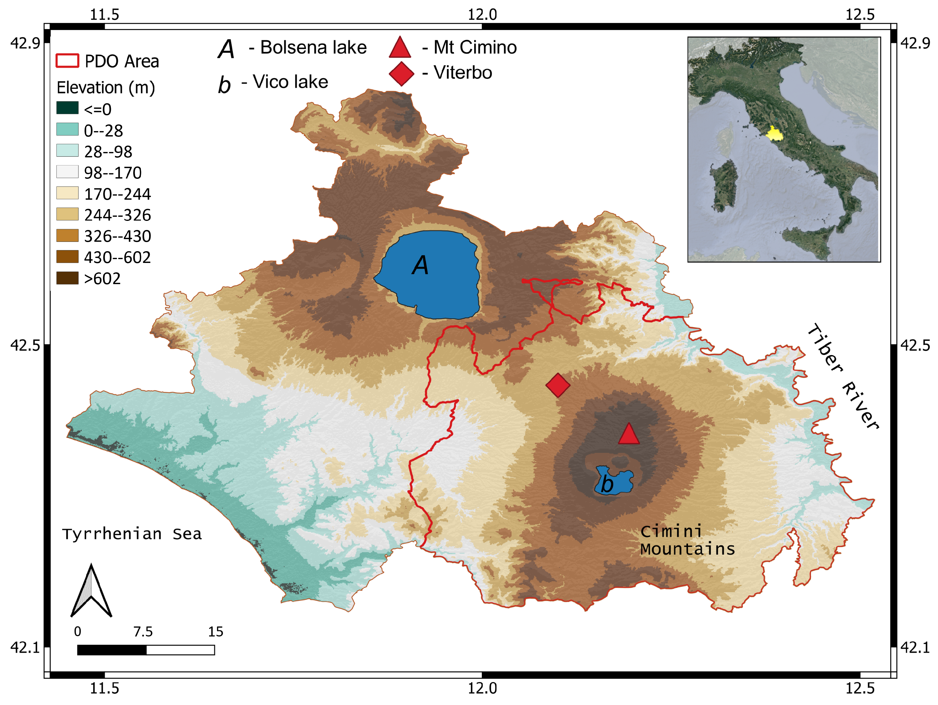
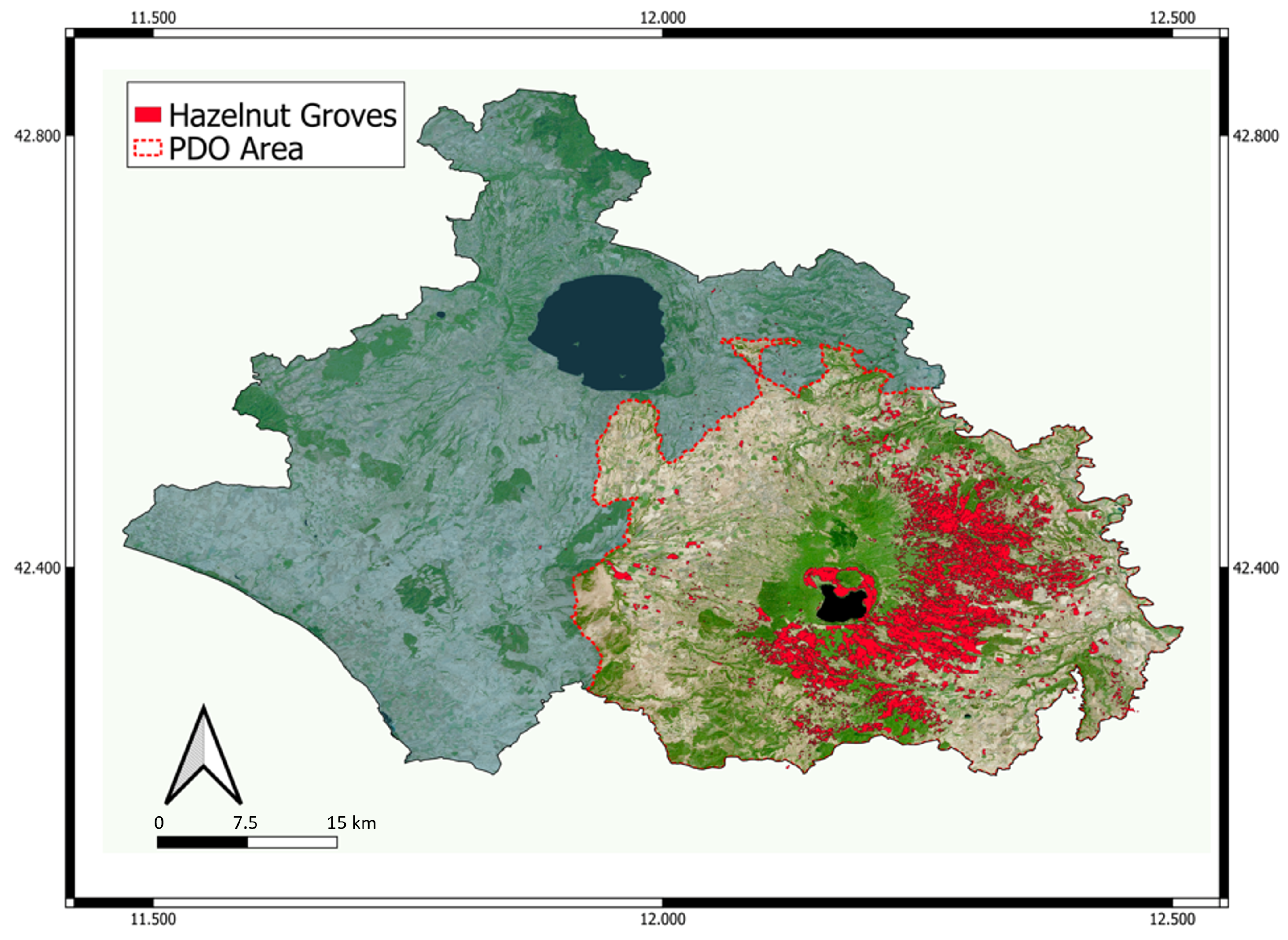
2.1. Study Area (AOI)

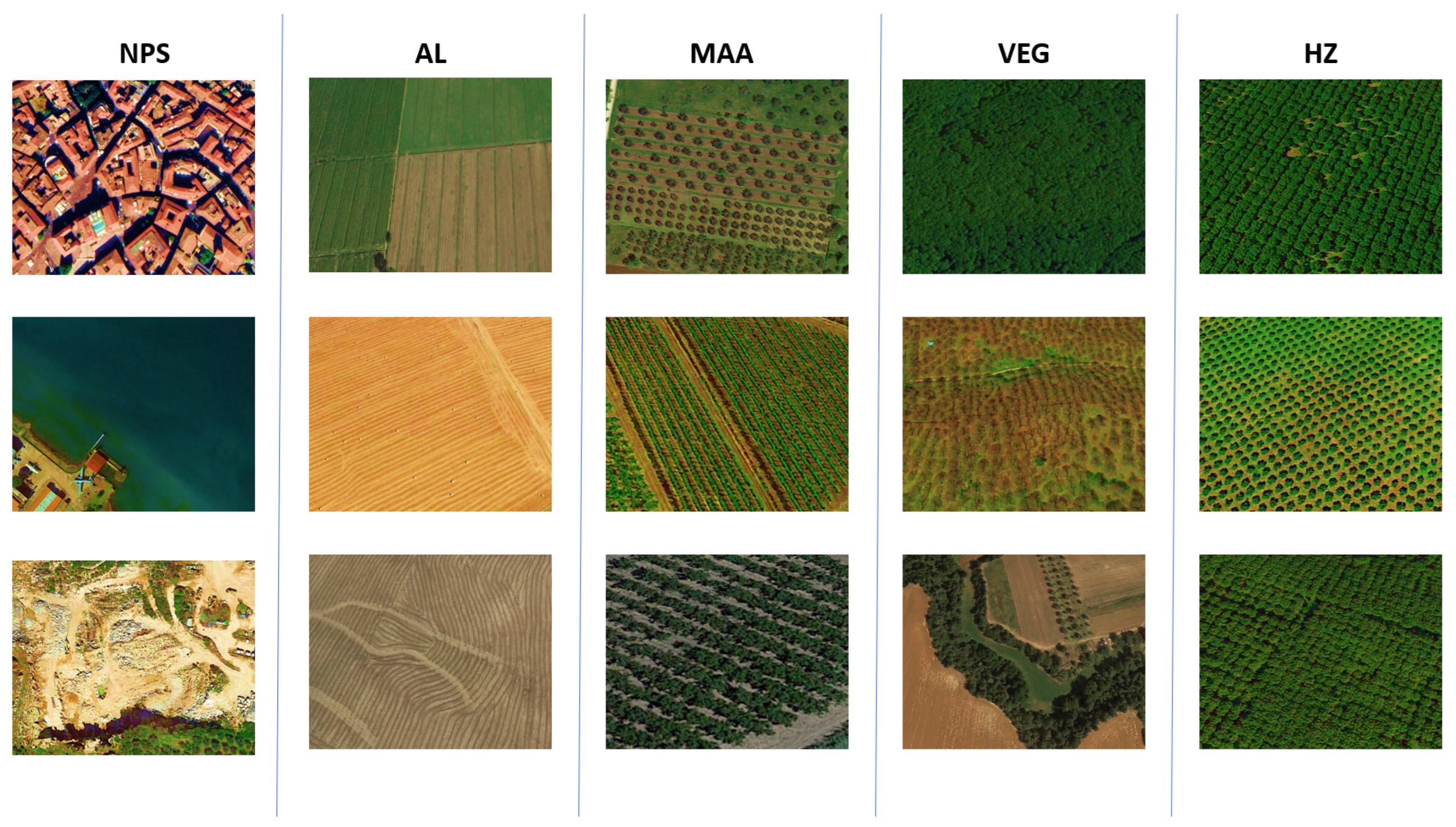
The study area corresponds to the administrative boundaries of the Viterbo province in Italy (Figure 1), covering approximately 3615 square kilometers. Geologically, the area can be divided into a coastal sector with gentle slopes renowned for horticultural and olive oil production, and an inland hilly sector of volcanic origin, characterized by the remnants of extinct volcanic structures. Within this region, there are three distinct lakes occupying the volcanic crater. The elevations in this area reach a maximum of 1000 m and are covered by extensive forest systems of diverse mix, including vast expanses of chestnut trees, oaks, beeches and wild hazelnuts [57].

The two hilly complexes are known as Monti Sabatini and Monti Cimini, with the latter being the focal area for Protected Designation of Origin (PDO) hazelnuts of Viterbo, named “Nocciola Romana”. The hazelnut cultivar typically grown in these zones is “Tonda Gentile Romana”, with small quantities of the “Nocchione” variety. Hazelnut cultivation in this region is typically carried out using a multi-stemmed bush system, with a density of approximately 500 (5 × 5 m inter and intra-row) trees per hectare; however, there has been a recent trend of establishing higher-density plantations [58]. In some areas, hazelnut groves 30 years of age with large plants are present. Periodically, hazelnut groves undergo pruning [59], which reduces canopy volume and can cause variation in reflectance due to the spectral mixing of soil and wood pixel signatures. The hazelnut is a deciduous plant, with an active vegetative growth phase during summer months, where irrigation intervention is often required, while pruning occurs during the vegetative rest period. These phenological parameters may vary based on the cultivar, environmental conditions, and diverse management practices.

2.2. Ground Truth

For ground truth data, Google Earth was exploited via WMS (Web Map Service) within the QGIS desktop free/open-source platform. Using high-resolution images (April 2022), supplemented by historical imagery from Google Earth Pro and extensive knowledge of the territory, 14,611 sampling points were selected within the AOI across various altitude bands and geographical arrangements to reduce spatial autocorrelation [60]. For the purpose of the study, five different land use categories were identified (Figure 2):

1.

Non-Photosynthetic Surfaces (NPSs), including urban areas, bare soils, rocks, and water bodies (1168 points).

2.

Arable Lands (AL), extensive areas devoted to arable farming or annual crop cultivation, characterized by the absence of arboreal vegetation (3016 points).

3.

Mixed Agricultural Areas (MAAs), encompassing tree vegetation associated with olive groves, vineyards, and various types of fruit orchards with diverse management practices (3060 points).

4.

Vegetation (VEG), represent areas covered by varying degrees of woodland vegetation. Spontaneous vegetation, woodland, coppices, chestnut groves, riparian areas, and scattered vegetation were included. This class encompasses a wide range of habitats, from Mediterranean scrub to garigue, evergreen and deciduous oak forests, pine groves, and beech woods (4374 points).

5.

Hazelnuts (HZs), comprising mature hazelnut plantations (>5 years) (2993 points).

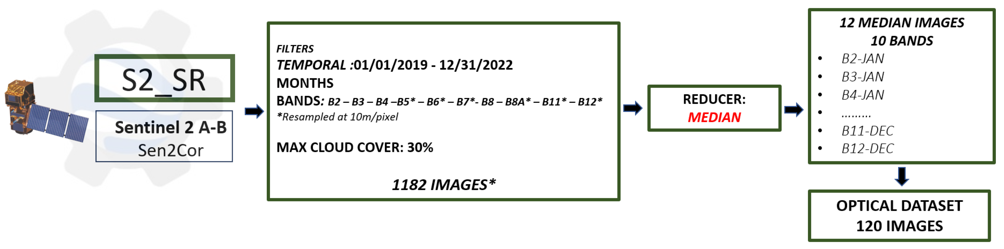
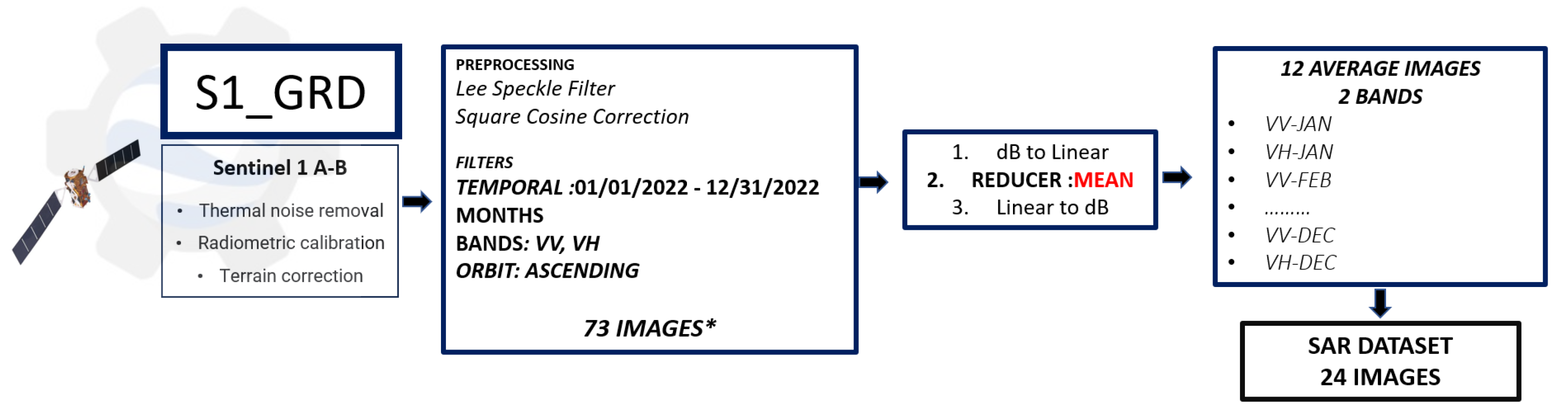
2.3. Satellite Data

For satellite data, we opted to use Sentinel-2, Sentinel-1, and a DEM (Digital Elevation Model) layer. The data were acquired through GEE, and all subsequent analyses were processed using the GeeMap package [61]. The choice of these satellites is primarily driven by the optimal compromise between spatial, spectral, and temporal resolutions, making them ideal for crop-monitoring applications. Additionally, their availability in GEE further contributes to their suitability and accessibility.

Sentinel-2 is a constellation comprising two passive optical satellites that operate in a sun-synchronous orbit, capturing data every 3–5 days at medium latitudes. It offers a spatial resolution of 10 m/pixel for RGB and Near Infrared (NIR) bands [62]. This satellite excels in discriminating surface spectral responses, utilizing specific bands targeted at vegetation, such as Red-Edge, NIR, and Short Wave Infrared (SWIR), with a great potential for estimation of the biophysical variables of canopies [63].

In the present study, the following bands were exploited:

• 4 × 10 m Bands: the three classical RGB bands (B2, B3, B4) and a Near Infra-Red (B8∼833 nm) band.
• 6 × 20 m Bands: 4 narrow bands in the VNIR vegetation Red-Edge spectral domain (B5∼704 nm, B6∼740 nm, B7∼783 nm and B8a∼865 nm) and 2 wider SWIR bands (B11∼1610 nm and B12∼2190 nm) for applications such as vegetation moisture stress assessment.

Sentinel-1 is a C-band synthetic-aperture radar (SAR) satellite system that comprises two active satellites, Sentinel-1A and Sentinel-1B. These satellites acquire data in all weather conditions, both during the day and night, with a revisital time of 6–12 days. They employ various modes and polarizations [64], enabling sensitivity to the dielectric constants of materials, including the water content and phenological stage of vegetation [65]. Additionally, the cross-polarization capability allows for the characterization of volumetric scattering, providing insights into the volume of biomass present in the observed area. These features make it highly suitable for crop identification and characterization [66,67,68].

The supplementary selection of the Digital Elevation Model (DEM) is employed to justify the temporal shift that can occur between bands at different altitudes, especially when observing the same type of vegetation cover. This is attributed to the variations in phenological phases that may affect the spectral–temporal response of the vegetation over different elevations [69].

2.3.1. Sentinel 2 Pre-Processing

To acquire optical data (Figure 3), Sentinel-2 surface reflectance data in Google Earth Engine (GEE) were employed. The S2_SR collection comprises geometrically and atmospherically corrected (Level-2A) satellite images from Sentinels A and B, processed with the Sen2Cor model [70]. The data selection focused solely on the Area of Interest (AOI), including images from 2019 to 2022, with a maximum 30% cloud cover threshold. The resulting image collection comprised 1182 images, either partially or entirely covering the AOI. The image collection was subdivided into monthly subsets, and median values were computed for RGB bands (B2, B3, B4), Red-Edge/NIR bands (B5, B6, B7, B8, B8A), and SWIR bands (B11, B12), all at a 10 m/pixel resolution. Nearest-neighbor interpolation was applied to bands B5, B6, B7, B8A, B11, and B12 for resampling to a 10 m resolution. Due to the coarse resolution of bands B1, B9, and B10, these bands were excluded from the analysis.

The choice of a 4-year timeframe was driven by the dynamic nature of agricultural systems, where annual anomalies may arise due to localized or widespread environmental factors, attributed to natural causes or specific management practices (e.g., intensive pruning and drought).

The use of median values for the monthly aggregation is particularly advantageous in mitigating the potential impact of outliers that might be present in the data. In the case of passive sensors such as Sentinel-2, these variations are often attributed to cloud cover [71], which can lead to anomalous pixel reflectance values. This approach can enhance the reliability of the land-use classification process, providing a more accurate representation of the AOI temporal dynamics. However, it is worth noting that this approach may not capture young hazelnut orchards (<4 years old), which would be particularly challenging, given the spatial resolution limitations. The optical dataset thus consists of 12 monthly median images, each containing 10 bands, for a total of 120 features.

2.3.2. Sentinel 1 Pre-Processing

For SAR data (Figure 4), the GEE Copernicus/S1_GRD (Ground Range Detected) dataset in IW (Interferometric Wide-swath) mode was utilized. Data were pre-processed with the Sentinel 1-Toolbox [72], including orthorectification, radiometric and thermal correction, expressed in decibels, and projected onto a regular 10 m grid. The acquired images over the Area of interest (AOI) for 12 months (from January 2022 to December 2022) were filtered by selecting the VV and VH polarization. Due to the considerably different viewing orientations between the ascending and descending satellite overpasses, only the ascending orbit was selected for this study to maintain data consistency. The resulting dataset consists of 73 images, preprocessed using the methodology of [66] with some adaptations. The data acquired from the different orbits were treated as distinct datasets, with a focus on selecting only the acquisitions with ascending orbits. To reduce speckle noise while preserving important image details, we applied the Lee Filter using a 3 × 3 pixel configuration. To address the effects of incidence angle variations on the backscatter, we implemented the Square Cosine Correction based on the Lambert law. This correction is based on the mean incidence angle of each image cropped on the Area of Interest (AOI) and serves as a reference angle. The subsequent steps involve value conversion into the linear unit, followed by monthly averaging, and finally converting the data back to decibels.

The choice to use data from the latest year (2022) aims to identify significant backscattering variations linked to recent events like extensive eradication activities. These changes might not be apparent when looking at median or average data over a four-year period. This process resulted in 12 average images, each with two frequency bands, totaling 24 features representing the SAR dataset.

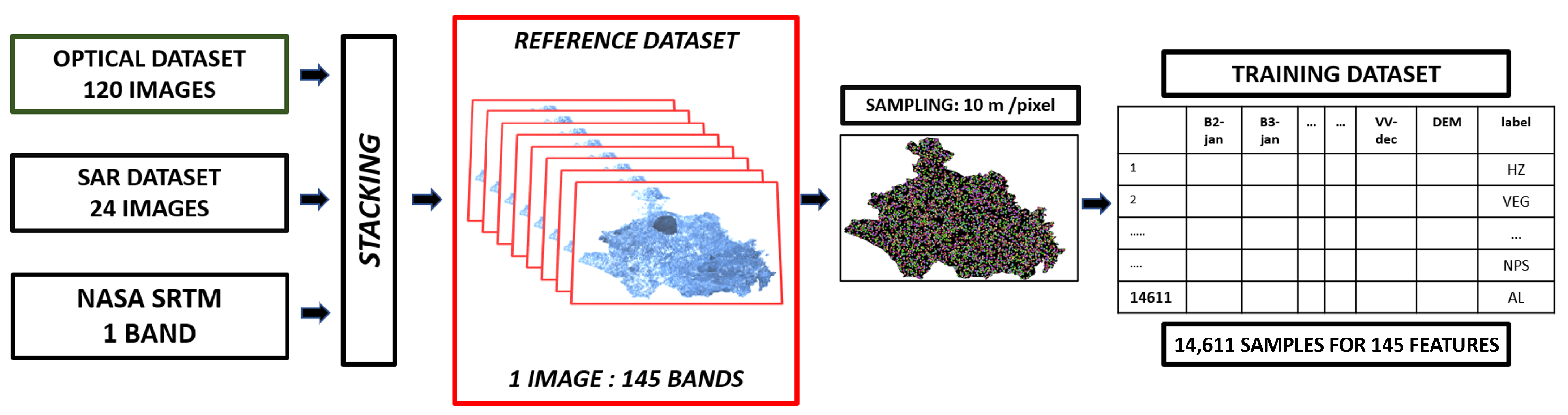
2.3.3. Digital Elevation Model (DEM)

The Shuttle Radar Topography Mission (SRTM) Global 1 arc-second digital elevation model (DEM) is an extensive global elevation dataset providing a resolution of approximately 30 m [73]. It was derived through single-pass interferometry during the space shuttle Endeavour mission in February 2000. The SRTM dataset was processed using the Google Earth Engine (GEE) platform, where it was cropped within the Area of Interest (AOI).

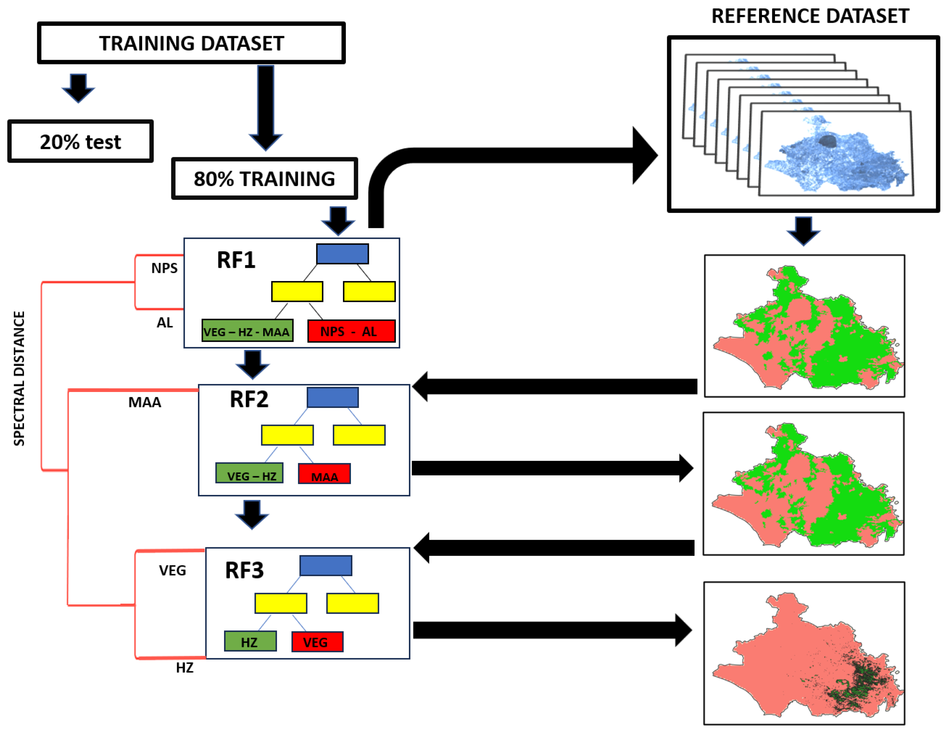
2.4. Reference and Training Datasets

After pre-processing the SAR and OPTICAL dataset, they were stacked into a spectral–temporal cube, incorporating the DEM band, and then cropped to cover AOI. The resulting reference dataset for classification consists in a dense cube of 145 bands. Out of these, 120 bands represent the median of 10 Sentinel-2 bands for each of the 12 months, 24 bands represent the average VV and VH bands of Sentinel-1 for 12 months, and one additional band represents the DEM layer. The summary of the data used for the reference dataset can be found in (

Table 1. Summary of the data used.

Data Source	Sentinel-2	Sentinel-1	DEM
EE-Collection	S2_SR	S1_GRD	SRTMGL1_003
Bands	B2, B3, B4, B5, B6, B7, B8, B8A, B11, B12	VV, VH	elevation
Filters	Max 10% Tile Cloud Cover	Orbit: ASCENDING	-
	01/Jan/2020 - 31/Dec/2022	01/Jan/2022 - 31/Dec/2022	-
N. Images	1182	73	1
Reducer	Median, Monthly	Average, Monthly	-

).

The training points were exported from the QGIS environment to Google Earth Engine (GEE), where a sampling on the reference dataset was performed at 10 m pixel resolution. Consequently, the training dataset comprises 145 features and 14,611 observations, each containing a specific label and the corresponding spectral–temporal signature (Figure 5). In this dataset, a stratified random sampling technique was employed to extract 20% of the observations for each land cover class. These extracted samples were intentionally not used during the model training process. Instead, they were reserved exclusively for the subsequent testing phase to ensure an unbiased evaluation of model performance [74].

To assess the contribution of individual bands in the classification process, vegetation indices were excluded from the analysis. While these indices have the potential to reduce dataset dimensionality while preserving crucial information, they were intentionally omitted to identify a specific group of spectral bands during a particular phase of the year, facilitating the differentiation between hazelnut groves and other land cover types.

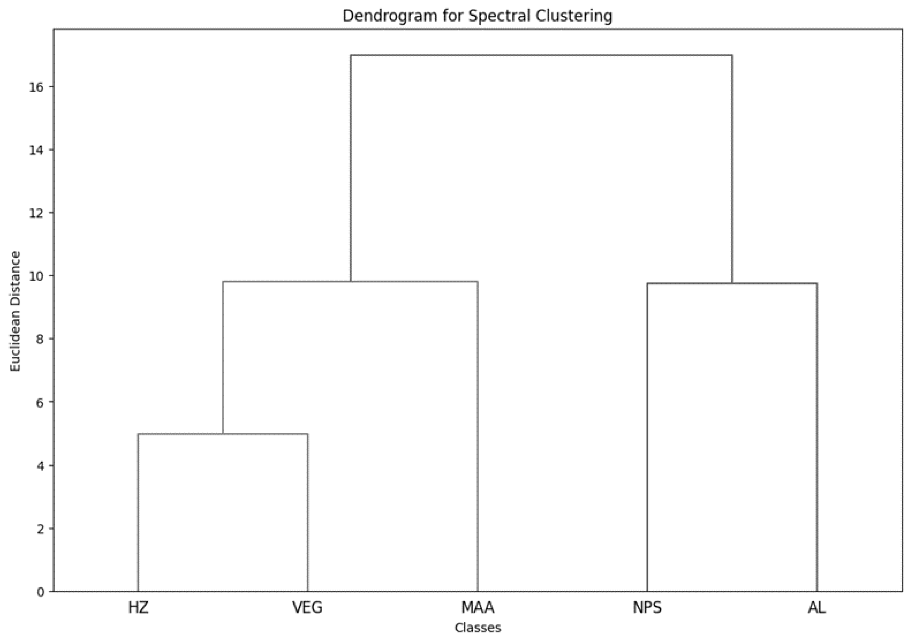
2.5. Spectral Separability Analysis

After creating the training dataset, a spectral separability analysis was conducted on the normalized median signatures of each land cover class. For each specific land cover class, the median spectral–temporal signatures were computed; subsequently, the values for each individual feature were subjected to normalization through the employment of a Min-Max scaler, thereby constraining them within the range of 0 to 1. This analysis identified clusters used as the foundation for training a series of Hierarchical Random Forest algorithms.

To achieve this, the data for each class were compared using a hierarchical cluster analysis [75] approach based on Euclidean distance, identifying all nodes that effectively separated hazelnut (HZ) from other land cover types. The primary objective was to achieve the spectral and temporal separation of hazelnut (HZ) from the land cover class that exhibited the most similarity.

2.6. Models Training and Test

Due to the high number of correlated variables in the training dataset, the potential challenges of the curse of dimensionality and multicollinearity arise, impacting the interpretability and stability of traditional models. The selection of the RF algorithm [76] is well founded, as it is widely supported by a substantial body of literature. Numerous studies have demonstrated its efficacy in satellite data analysis and crop classification tasks [77,78,79] especially with a fused dataset [80]. Random Forest is particularly well suited for this study due to its robustness in handling high-dimensional datasets and addressing multicollinearity challenges. The ensemble nature of RF, which combines multiple decision trees through bagging, allows it to effectively manage a large number of variables. By employing different subsets of training data and features in each tree, RF mitigates the risk of overfitting, ensuring both high accuracy and good model generalization [81]. Moreover, RF excels at handling large volumes of data with linear and nonlinear structures as frequently encountered in satellite data [48], providing interpretable models and the explainability of variables through specific metrics [82,83]. The RF algorithm’s capability to handle high-dimensional datasets and correlated features makes it an optimal choice for our analysis, striking a balance between accuracy and computational efficiency. The methodology employed (Figure 6) involves using multiple RF classifiers, each trained at a specific hierarchical layer, to achieve accurate separation of hazelnut areas. For training the classifiers, optimal hyperparameters were searched using grid search and 10-fold cross-validation to maximize model performance at each step. At each step of the classification process, accuracy metrics such as overall accuracy, precision, recall, and F1-score were assessed to evaluate the model’s performance. These metrics were calculated both in cross-validation and on the separate 20% test dataset, to provide a comprehensive evaluation of the models’ performance using different sets of unseen data.

The trained models were applied to classify the entire reference dataset hierarchically, isolating a layer with only HZ instances. The resulting HZ classification layer underwent sieving (maximum 10 pixels, 4-connectivity) to reduce salt-and-pepper effects. Once the final raster classification was generated, the shape of the classified HZ area was vectorized and analyzed.

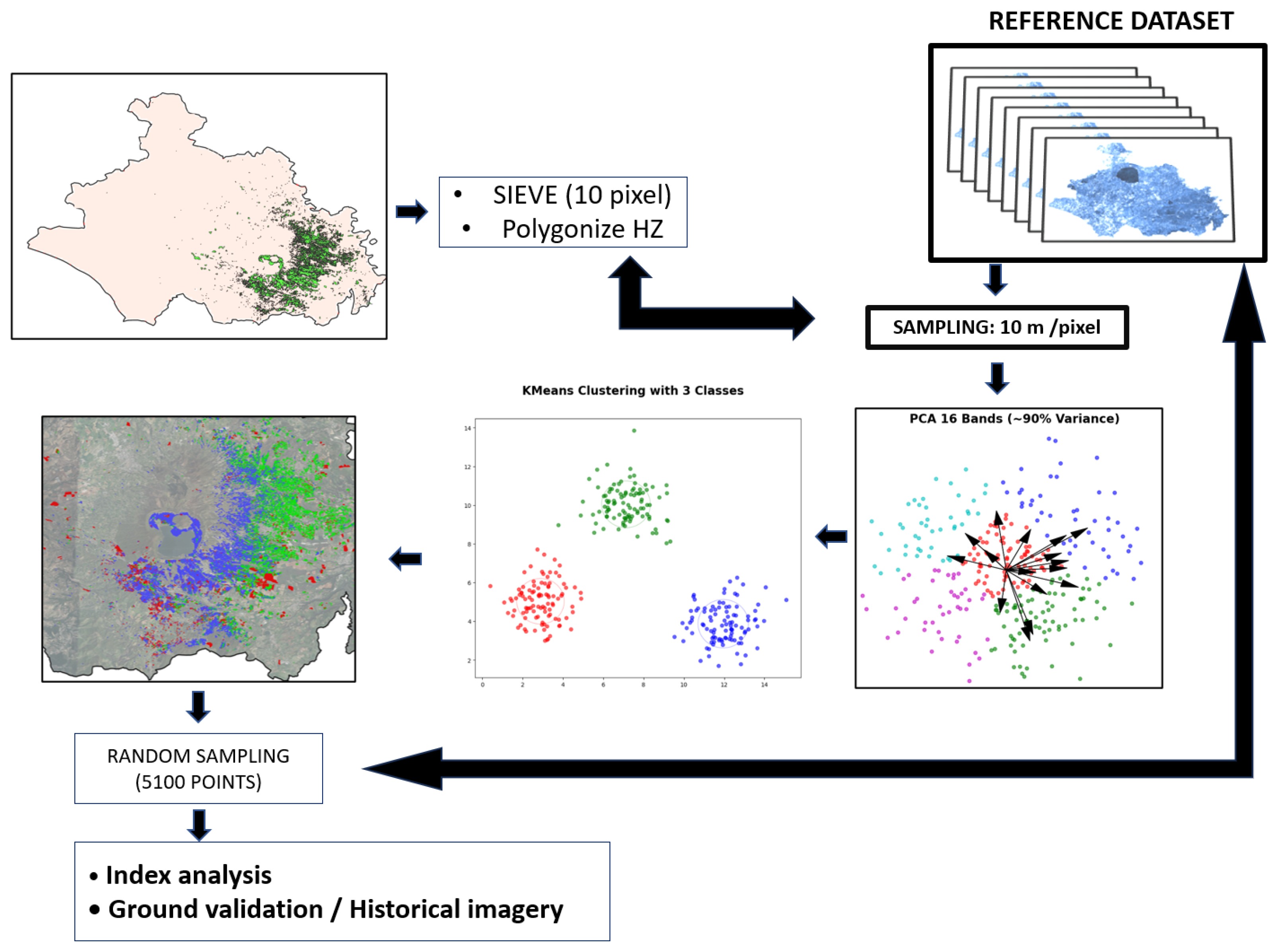
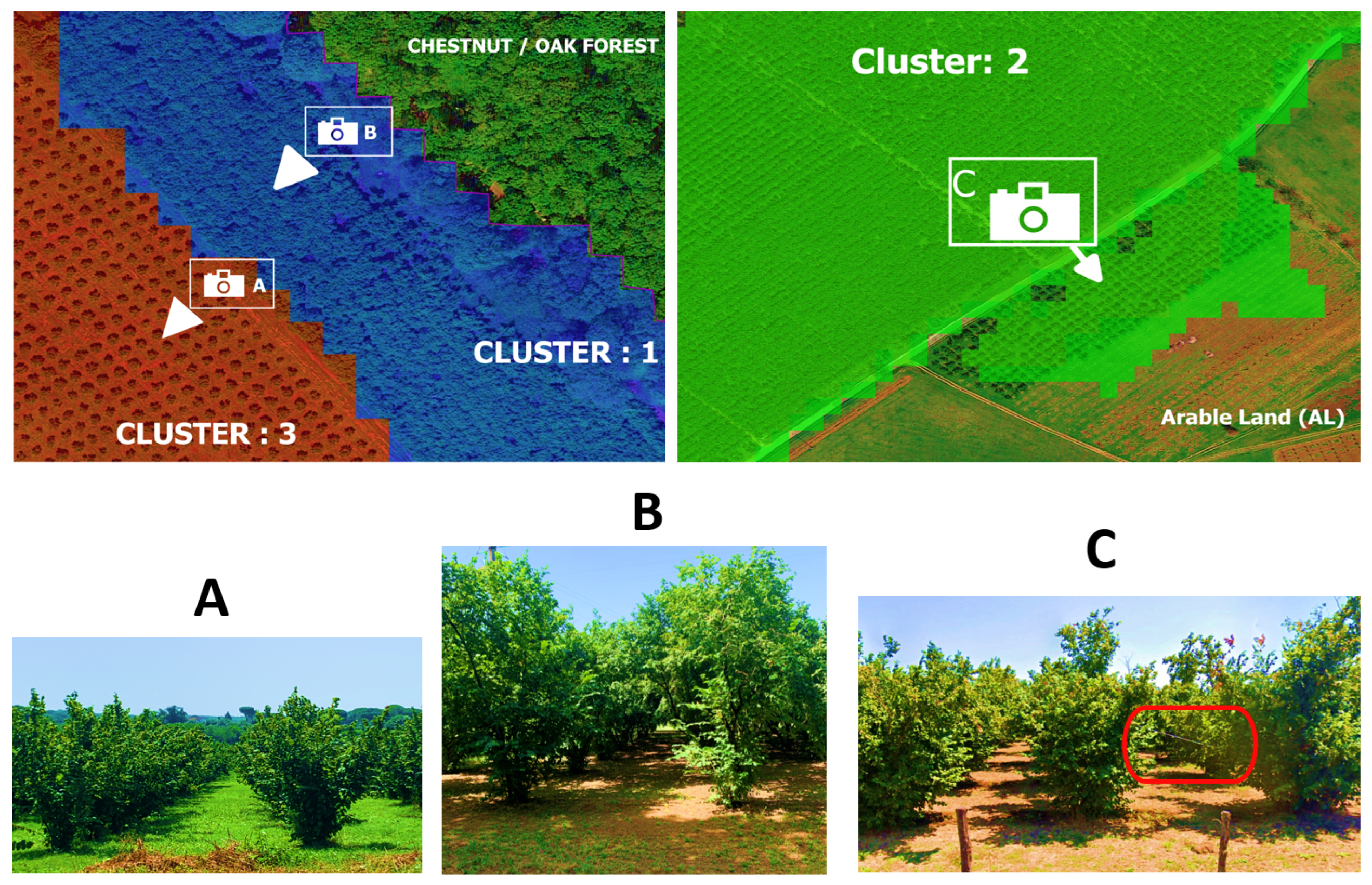
2.7. Hazelnut Groves Characterization

After delineating the hazelnut groves within the AOI, the spectral–temporal signature for each pixel falling within the HZ polygons was extracted from the 10 m/pixel reference dataset. The hazelnut-specific data were then normalized, and to address dimensionality and inter-band correlation, a Principal Component Analysis (PCA) was applied, selecting the minimum number of principal components that collectively accounted for at least 90% of the data variability. Once the principal components were obtained, the scores matrix underwent unsupervised clustering using K-means, in a framework similar to [84]. The appropriate number of clusters was identified using the elbow method [85] based on SSE (Sum of Squared Errors or Inertia), which computes the sum of squared distances of data points to their assigned cluster centroids. The method aims to identify the optimal number of clusters by examining the rate of change of SSE; a sharp change in the slope of the SSE curve indicates the elbow point, thus the optimal number of clusters. The resulting clusters were then projected back onto the AOI in QGIS, where the cluster-based classification was subjected to a 20-pixel sieve with 4-connectivity.

To provide interpretability to the clustering results (Figure 7), two approaches were followed:

• Ground validation and historical imagery.
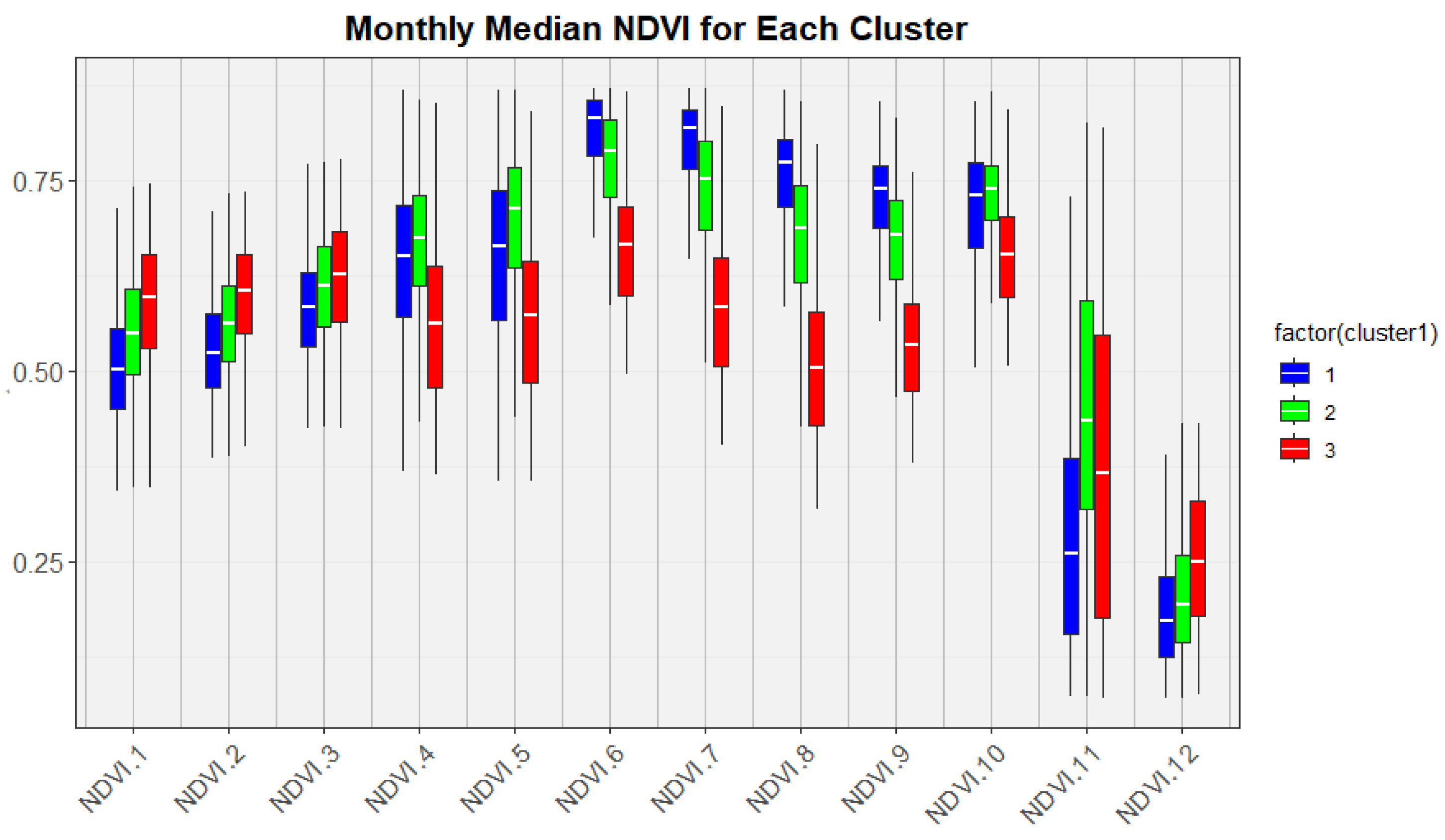
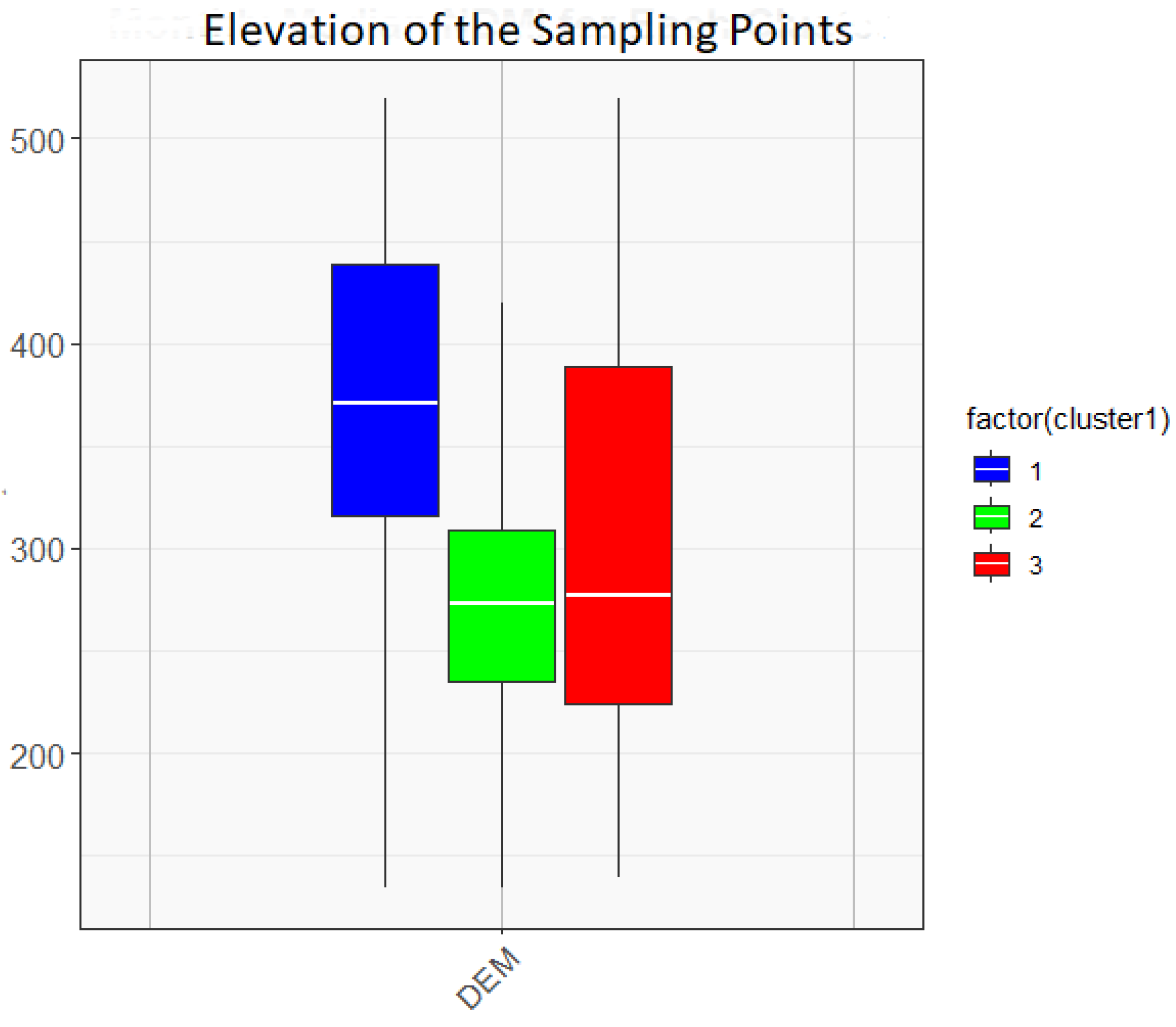
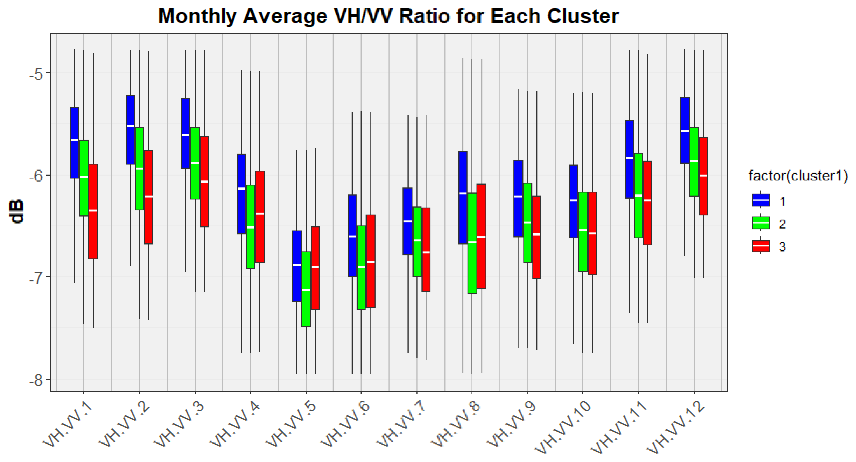
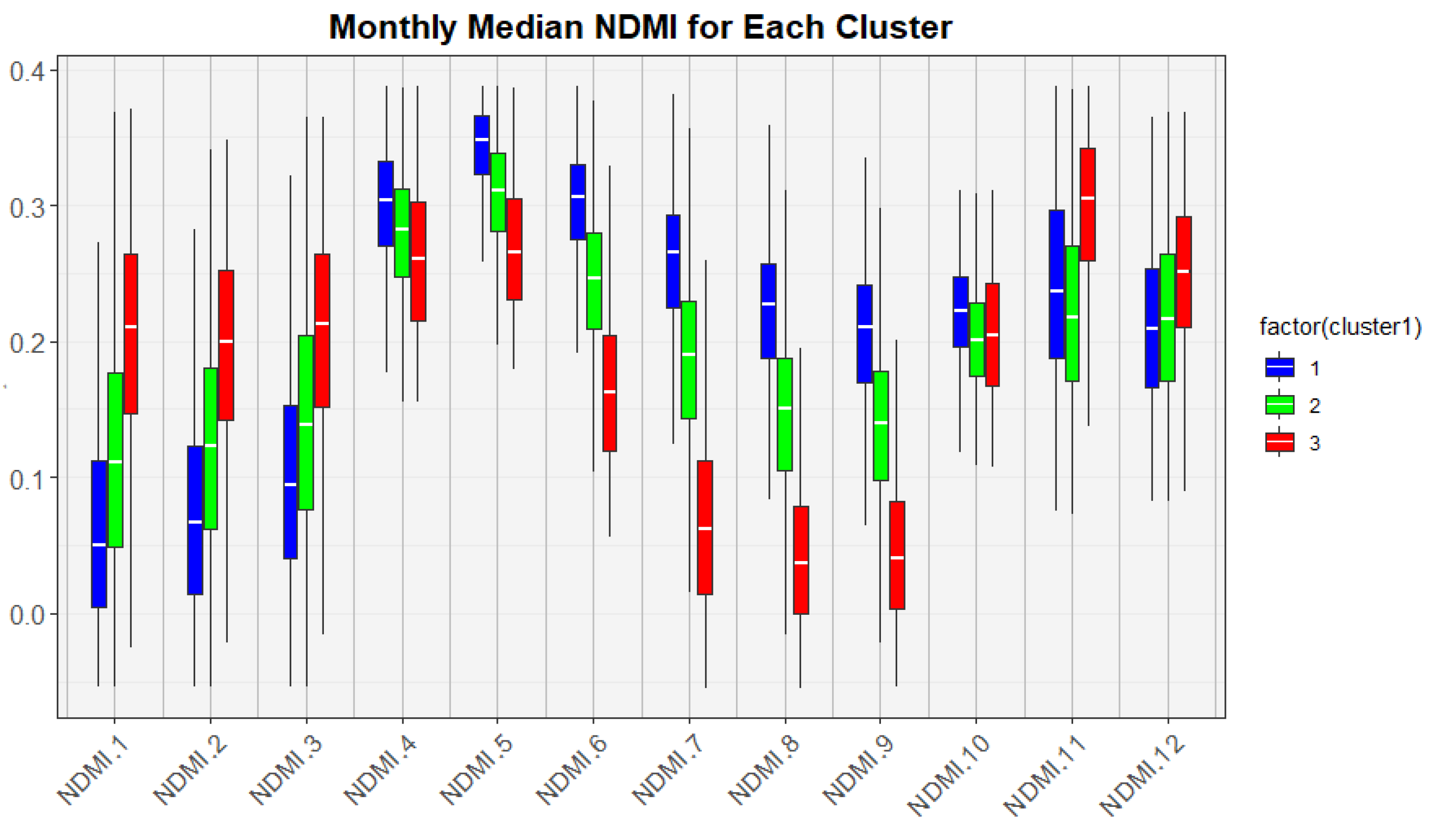
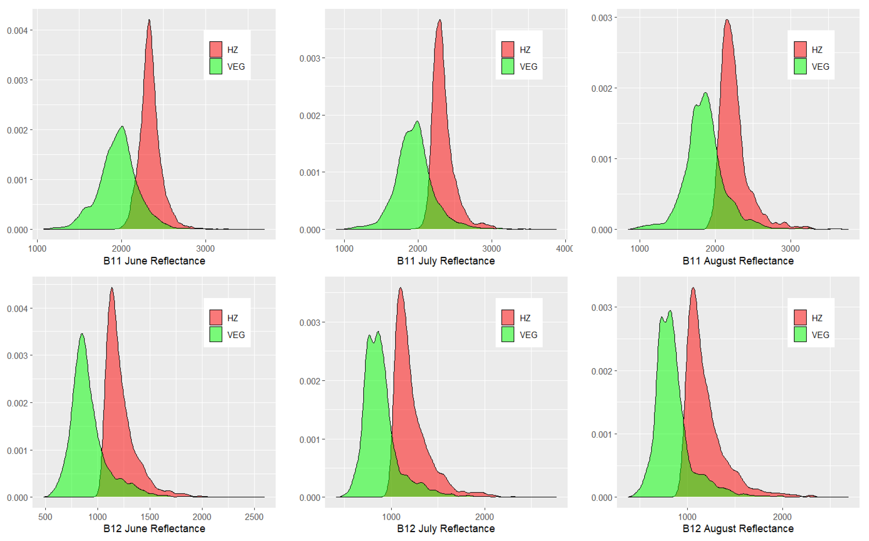
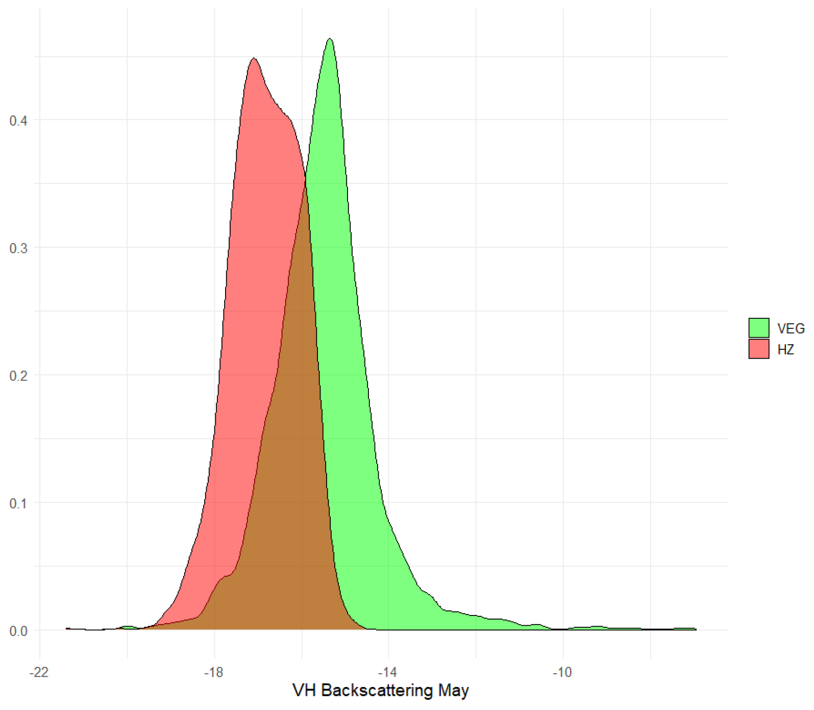
• Interpretation through indices: A total of 1700 random sampling points were placed within the polygons of each cluster, resulting in a total of 5100 sampling points. Spectral–temporal data were extracted from the reference dataset at these points, and three specific indices were applied to analyze and interpret the data. These indices (VH/VV ratio, NDVI, NDMI) are widely used in the literature to define phenological stages and biophysical parameters of vegetation [17,86,87].

The VH/VV ratio in decibels is given by:

$$\mathrm{VH}/\mathrm{VV}\mathrm{ratio}\left(\mathrm{dB}\right)=\mathrm{VH}\left(\mathrm{dB}\right)-\mathrm{VV}\left(\mathrm{dB}\right)$$

This index indicates the presence of structures capable of strengthening the VH signal in the presence of high entropy surfaces, such as canopies. Moreover, VV is influenced by leaf or soil water content, making this index indicative of biomass and water content [65].

The NDVI (Normalized Difference Vegetation Index), widely utilized for assessing vegetation health, is highly correlated with various biophysical parameters of vegetation [88]. It represents the normalized ratio between the NIR (Near-Infrared) and Red bands. In the case of Sentinel-2, it is given by:

$$\mathrm{NDVI}=\frac{\mathrm{B}8-\mathrm{B}4}{\mathrm{B}8+\mathrm{B}4}$$

The third index is the NDMI (Normalized Difference Moisture Index), used to estimate leaf water content. It utilizes the NIR and SWIR (Short-Wave Infrared) bands [89]. In the case of Sentinel-2, it is given by:

$$\mathrm{NDMI}=\frac{\mathrm{B}8-\mathrm{B}11}{\mathrm{B}8+\mathrm{B}11}$$

Moreover, an additional analysis was conducted on the DEM data for each random point within the different clusters. This analysis aimed to assess potential differences arising from a temporal shift in phenological phases associated with varying altitude bands.

3. Results

3.1. Spectral Separability Analysis

The analysis of spectral separability based on normalized median spectral–temporal signatures provided valuable insights into the similarity patterns among the land cover classes. The resulting distance matrix (

Table 2. Matrix of Euclidean distances on the normalized spectral–temporal signatures of different land covers.

	VEG	HZ	MAA	AL	NPS
VEG	0	3.4	5.7	9.5	8.9
HZ		0	5.7	8.0	8.5
MAA			0	6.4	7.6
AL				0	6.8
NPS					0

) illustrates the pairwise distances between the classes, calculated using the Euclidean distance metric.

The analysis based on the Euclidean distance metric revealed clear relationships among the land cover classes. Specifically, classes VEG and HZ demonstrated the highest similarity. Classes NPS and AL showed moderate similarity to each other but were distant from classes VEG, HZ, and MAA, with the latter displaying less separability from the VEG and HZ cluster. NPS and AL were distinctly separated from classes containing various types of tree vegetation (Figure 8).

The cluster analysis generated three levels of distinction for hazelnut grove discrimination. At the first level, a cluster separated NPS_AL from MAA_VEG_HZ. At the second level, another cluster distinguished MAA from VEG_HZ, and at the final level, a separate cluster isolated VEG from HZ. As a result, to train the different models, all observations for each cluster node were selectively filtered. Initially, AL and NPS were separated from MAA, VEG, and HZ (RF1). Subsequently, MAA was separated from VEG and HZ (RF2). Finally, all VEG observations were separated from HZ (RF3).

3.2. Model Performance on Training and Hyperparameters

The confusion matrices (

Table 3. Confusion matrix of the RF1 model on the training dataset.

RF1	NPS ∪ AL	VEG ∪ HZ ∪ MAA
NPS ∪ AL	3359	1
VEG ∪ HZ ∪ MAA	0	8328

,

Table 4. Confusion matrix of the RF2 model on the training dataset.

RF2	MAA	VEG ∪ HZ
MAA	2449	0
VEG ∪ HZ	0	5891

and

Table 5. Confusion matrix of the RF3 model on the training dataset.

RF3	HZ	VEG
HZ	2406	1
VEG	7	3478

) illustrate the cross-validation performance for each RF model, consistently achieving accuracy, precision, recall, and F1-scores above 0.99 with specific hyperparameters (

Table 6. Accuracy metrics and hyperparameters for RF1, RF2, and RF3 models on the training dataset. The results are averaged for both classes in each model. ES: Estimators (number of trees); MS: Minimum Samples for node splitting, MD: Max Depth.

Model Performance on Training Set	RF1	RF2	RF3
Overall Accuracy	0.99	1	0.99
Precision	0.99	1	0.99
Recall	0.99	1	0.99
F1-score	0.99	1	0.99
Hyperparameters	ES: 150 MS: 5 MD: 20	ES: 150 MS: 2 MD: 20	ES: 100 MS: 5 MD: 10

). The VEG-HZ classifier showed minimal false positives in the HZ class, with no significant impact on overall performance.

3.2.1. Model Performance on Test

In the testing phase, the models achieved high performance (

Table 7. Confusion matrix of the RF1 model on the test dataset.

RF1	NPS ∪ AL	VEG ∪ HZ ∪ MAA
NPS ∪ AL	822	2
VEG ∪ HZ ∪ MAA	10	2088

,

Table 8. Confusion matrix of the RF2 model on the test dataset.

RF2	MAA	VEG ∪ HZ
MAA	605	6
VEG ∪ HZ	13	1462

and

Table 9. Confusion matrix of the RF3 model on the test dataset.

RF3	HZ	VEG
HZ	584	2
VEG	2	822

) with overall accuracies, precision, recall, and F1-scores close to 1 (

Table 10. Accuracy metrics for RF1, RF2, and RF3 models, based on the average of both classes.

Model Performance on Test-Set	RF1	RF2	RF3
Overall Accuracy	0.99	0.99	0.99
Precision	0.99	0.99	0.99
Recall	0.99	0.99	0.99
F1-score	0.99	0.99	0.99

).

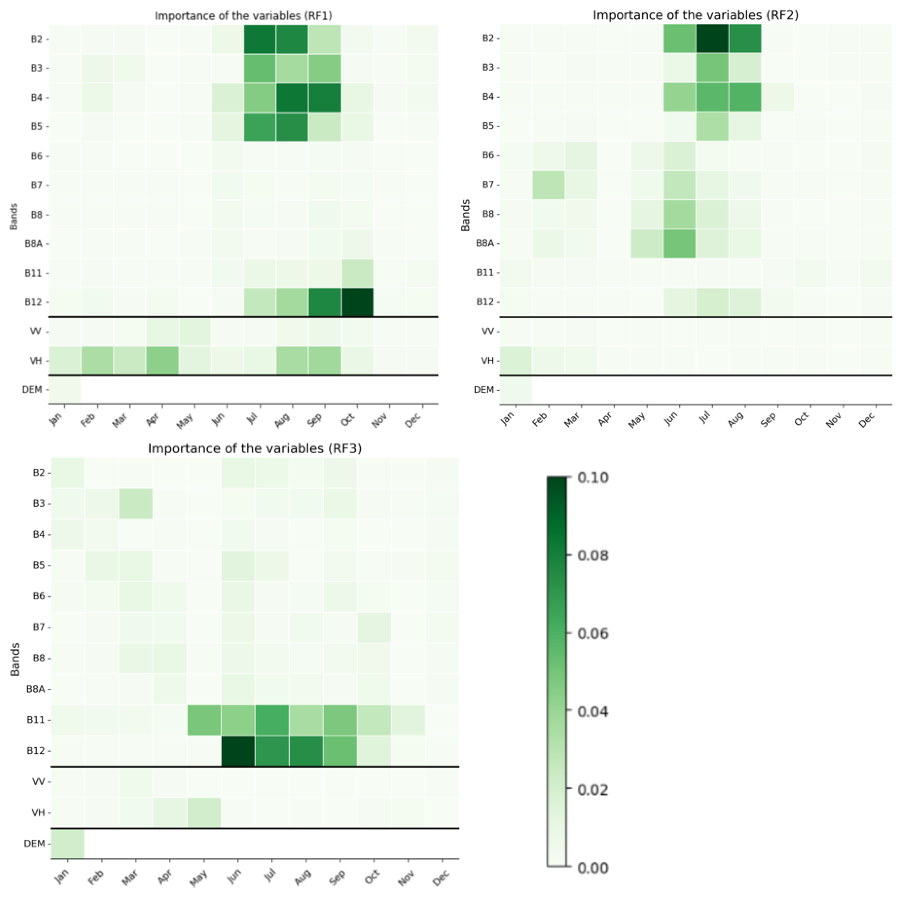
3.2.2. Importance of the Variables

The importance of features in the classifiers, evaluated via Mean Decrease in Impurity (MDI), is depicted in Figure 9. Generally, MDI values across classifiers do not exceed 0.1. For RF1, predominantly during the later summer months, notable importance can be observed in the B12 and visible bands. Within B12 (SWIR), the importance gradually increases during the summer months, reaching its peak in October. With regard to SAR data, the VH band appears to have greater importance than the VV band, albeit with irregular trends in different time segments throughout the year. The DEM data did not show a significant importance in the classification process.

In RF2 model, the features showing greater importance are also concentrated in the summer period, particularly in the visible spectrum region. In addition, some of the Red-Edge and NIR bands show importance at the beginning of the summer season. The SAR and DEM bands show lower MDI values, indicating a mild contribution to the classification process. Within the RF3 model, a clear pattern emerges, indicating that SWIR bands (B11 and B12) exhibit the most relevant MDI values, highly concentrated during the summer period. Conversely, other bands demonstrate comparatively diminished importance in the classification process.

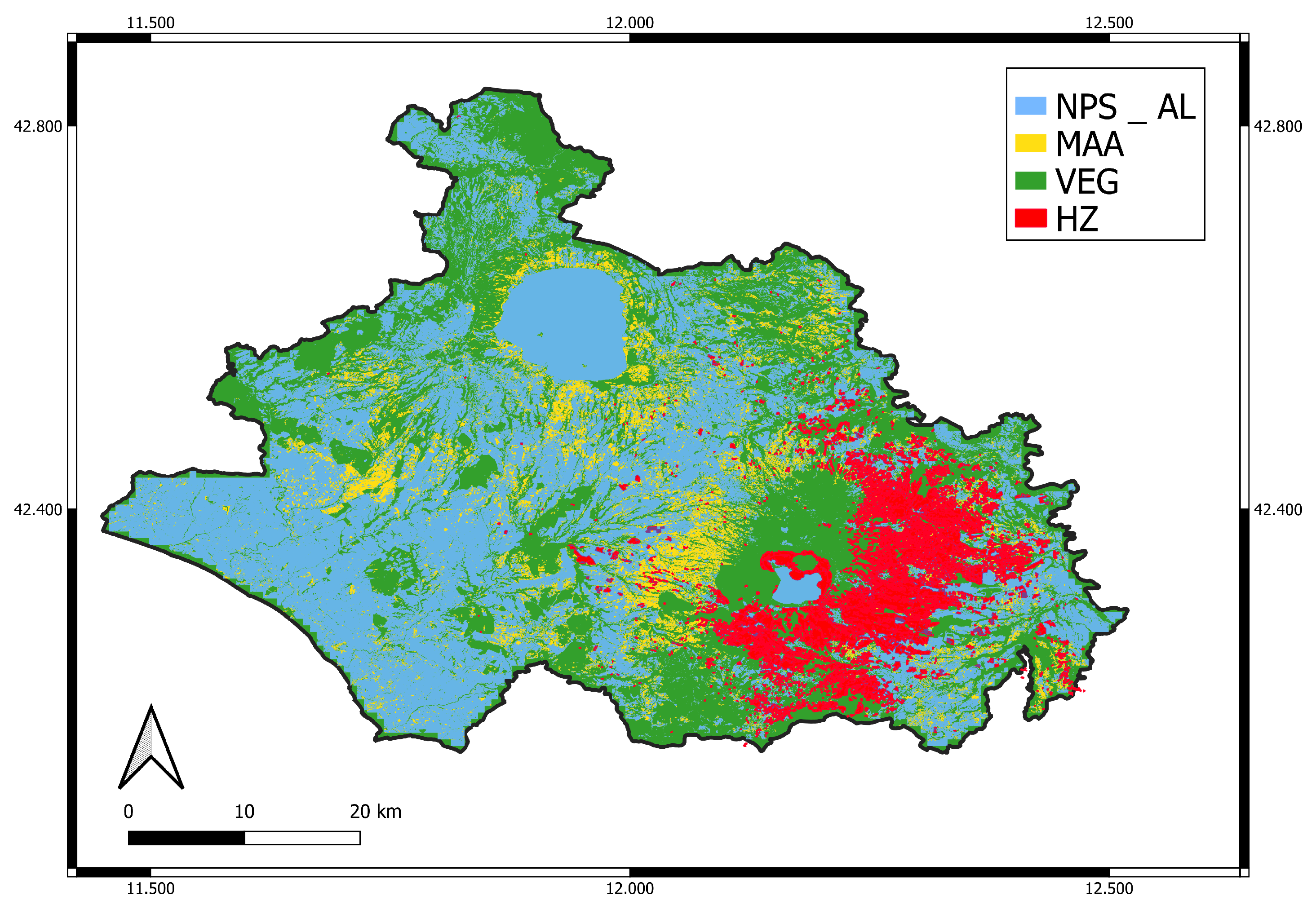
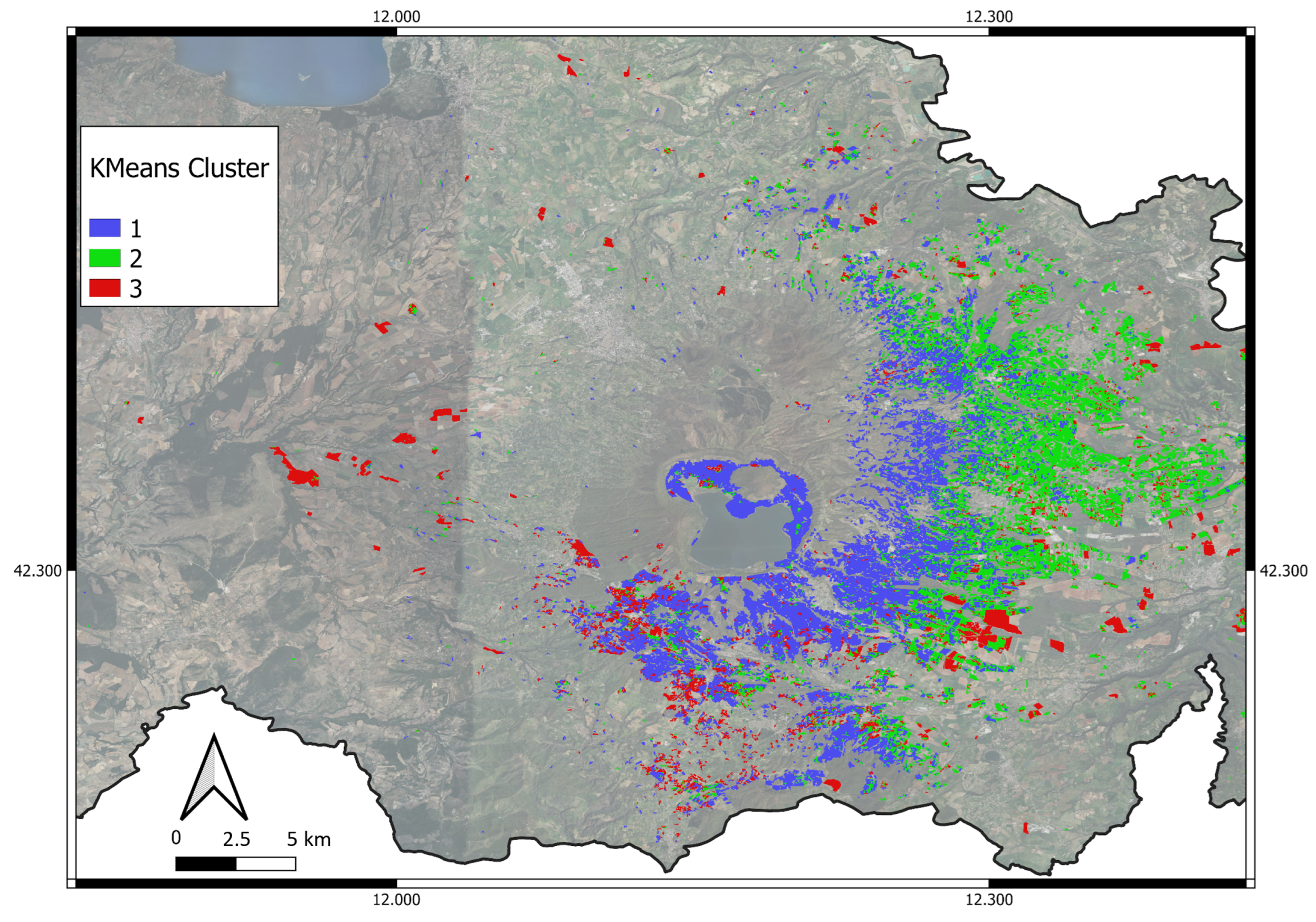
3.3. Classification on AOI

In Figure 10, the land cover classification of the AOI is presented. Along the Tyrrhenian Sea coastline, the dominant land cover is attributed to the NPS_AL class, outlining a landscape characterized by expansive arable fields and rural settlements. The discernible features of Lake Vico and Lake Bolsena contribute to the distinctiveness of this pattern.

Clusters of the MAA class are observed in specific regions, including the western flank of Mount Cimino and the peripheries of Lake Bolsena, showcasing a combination of vineyards and olive groves.

The VEG class is represented by large, scattered patches, encompassing diverse vegetation formations like Mediterranean maquis, garigue, and oak groves. This botanical continuum extends inland, featuring a notable prevalence of chestnut trees and other shrub-like species. Particularly in areas with pronounced topographical gradients unsuitable for conventional agriculture, these botanical constituents thrive. Importantly, the classification reveals branching, ramified configurations indicative of riparian vegetation within the overall vegetation mosaic.

Hazelnut Groves on AOI

The area occupied by HZ (Figure 11) forms a compact central nucleus, covering the eastern volcanic slope and the crater of Mount Cimino, with significant extensions around Lake Vico. Moving westward, the HZ extension significantly diminishes, primarily appearing as large fragmented fields, especially towards the coastal area and the city of Viterbo. After sieving, the predicted HZ area covers 22,780 hectares, of which 22,670 (99.5%) are located within the PDO area.

3.4. Characterization of HZ Polygon

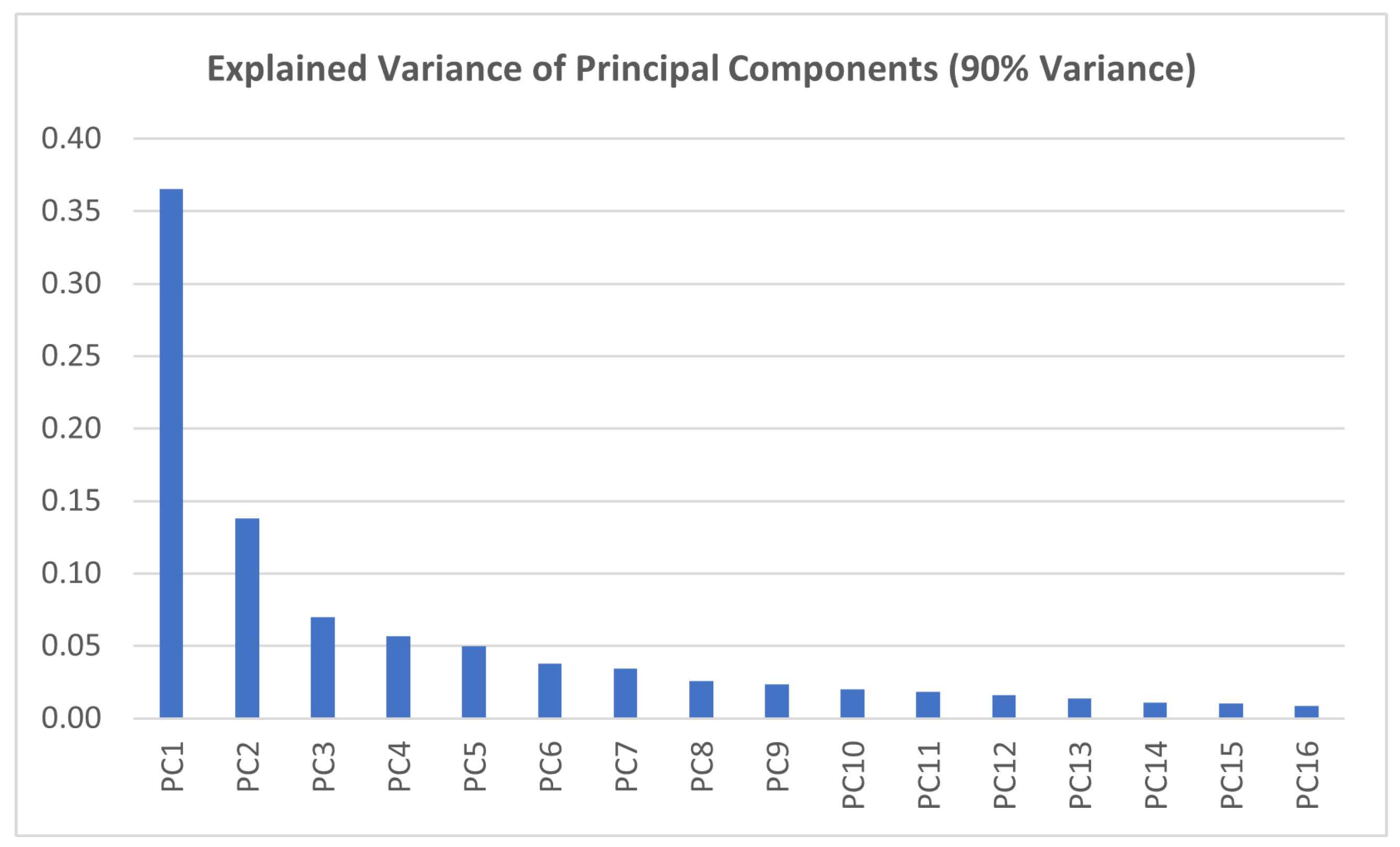
3.4.1. PCA and Cluster Identification

PCA analysis revealed that 16 principal components are necessary to capture 90% of the HZ spectral–temporal data variability (Figure 12). Subsequently, score matrices were generated for each of the 16 principal components and pixels, and these matrices were subjected to the elbow method (Figure 13) to assess the optimal number of clusters, determined to be N = 3.

Consequently, a K-means algorithm with three clusters was applied to the reduced dataset, assigning each pixel its corresponding cluster number as depicted in Figure 14.

3.4.2. Clusters Analysis

The boxplots illustrating the VH/VV ratio (Figure 15) for different clusters reveal a consistent temporal pattern across all clusters. Particularly, there is a distinct rise in the discrepancy between the two bands during late spring and summer, followed by a gradual increase in the index during autumn and winter. Analyzing individual clusters, Cluster 1 consistently exhibits a higher prevalence of the VH band over VV compared to Clusters 2 and 3, both of which show a similar trend and comparable medians.

Concerning the NDVI index (Figure 16), distinct temporal patterns are observed. Cluster 3 consistently maintains uniform median values throughout the year, experiencing a rapid decline in the index during November and December. Cluster 3 demonstrates higher index values during winter compared to Clusters 1 and 2 but significantly lower values during the summer period. In contrast, Clusters 1 and 2 follow a more analogous temporal trajectory, with values peaking during the summer and experiencing a sharp decline in late autumn. It is noteworthy that Cluster 2 maintains higher median values compared to Cluster 1, except during the summer months, when Cluster 1 exhibits a substantially higher value.

Regarding the NDMI index (Figure 17), all clusters show a similar temporal trend characterized by two distinct peaks during spring and late autumn, with a subsequent decrease during the early months of the year and in the summer. Concerning the individual clusters, Cluster 3 displays higher values compared to Clusters 1 and 2 during the initial and final months of the year, while being markedly lower during the summer period. Clusters 1 and 2 demonstrate a pronounced peak in spring and early summer, with the median value of Cluster 1 being consistently higher than Cluster 2 during this period, while the latter exhibits higher values during the winter months.

From the analysis of elevation data at random sampling points within the different clusters (Figure 18), higher values of Cluster 1 can be observed compared to Clusters 2 and 3, which are more similar. However, when examining the overall data distribution using boxplots, considerable variability is evident in Cluster 3.

The non-parametric Kruskal–Wallis test was employed to examine statistically significant differences in the elevation of sampling points, as the data deviated from normality assumptions. The consistently low p-values, approaching zero, provide robust evidence for rejecting the null hypothesis of equal altitude distributions (

Table 11. Results of the Kruskal–Wallis test for altitude comparisons among clusters.

Comparison	n	Statistic	p
Cluster 1 vs. Cluster 2	3400	1283	5.01 × ${10}^{-281}$
Cluster 1 vs. Cluster 3	3400	506	3.90 × ${10}^{-112}$
Cluster 2 vs. Cluster 3	3400	55.6	8.81 × ${10}^{-14}$

).

4. Discussion

4.1. Model Performance Results and Classification of AOI

The spectral analysis reveals clear separability among land cover types. Specifically, NPS surfaces exhibit spectral dissimilarity compared to arboreal vegetation but demonstrate proximity to arable or plowed fields (AL), likely influenced by post-harvest periods affecting the spectral signature, akin to artificial surfaces [90].

The MAA cluster shows closer proximity to VEG and HZ, attributed to prevalent olive groves with irregular planting patterns. This results in significant exposed bare ground, influencing pixel spectral signatures while retaining arboreal vegetation coverage. VEG and HZ, characterized by compact and uniform tree coverage with substantial canopy development, exhibit higher similarity. Differences in phenological phases may significantly impact spectral–temporal signature similarities between VEG, HZ, and MAA [91].

The performance of the RF models and the hierarchical workflow employed is excellent, both during cross-validation and testing on independent samples in the training process. The models consistently achieve average accuracies, precisions, recalls, and F1-scores exceeding 0.99. The hierarchical approach highlights how optimal hyperparameter search and cross-validation lead to specific and generalized models, effectively discriminating nested categories, such as the HZ class within VEG.

The study highlights the crucial influence of summer months on spectral–temporal classification. The NIR and Red-Edge bands show limited significance in RF1, aligning with prior research [92]; on the other hand, significant importance is attributed to the B12 band (SWIR). The combined NPS ∪ AL clusters exhibit heightened reflectance in the visible band, attributed to high reflectivity from soil and artificial surfaces, distinguishing them from vegetated regions [93]. In RF1, radar-derived parameters, particularly VH, strongly influence outcomes, reflecting the high entropy scattering of vegetated tree surfaces [94] with respect to flat surfaces as AL.

RF2 also underscores the importance of visible bands, especially during summer, in distinguishing MAA from VEG ∪ HZ. The spectral–temporal signature of MAA, which includes olive groves and vineyards, appears influenced by visible soil due to inter-row spacing in olive groves and due to biomass reduction during summer thinning in vineyards. SWIR, DEM, and SAR variables show limited importance in this classification step. RF3 underscores the significance of SWIR variables during summer, indicating a lower leaf water content in hazelnut groves compared to spontaneous vegetation (Figure 19). This could be attributed to the hazelnut’s limited ability to regulate stomatal conductance during thermal stress [89]. The discernible difference among SWIR variables during the summer period might indicate a distinctive characteristic for distinguishing hazelnuts from natural vegetation.

The importance of SAR variables in the classification process is limited to the initial stage (RF1), and in the month of May for RF3, where hazelnut showed a lower VH backscattering compared to the spontaneous vegetation (Figure 20). This is probably due to mowing and weeding operations that take place in this month in the inter-row spaces.

However, the general importance across all variables and classifiers is consistently low, typically ranging from 0 to 0.1. Consequently, while certain variables may exhibit slightly higher significance, the cumulative contribution of all features makes specific feature selection less pivotal in this work context.

After the sieving process, the ultimate AOI classification indicates a hazelnut coverage of 22,780 hectares, in close accordance with national statistics, which reported 23,900 hectares in total and 21,700 hectares in production for the year 2022. The mapping delineates hazelnut groves primarily within the PDO area (99.5%). Intensive cultivation is observed in the Monte Cimino area, especially around the volcanic crater of Lake Vico, with extensive and compact extensions on the eastern and southern slopes. The western flank exhibits mixed agricultural systems with hazelnuts facing environmental and social constraints. Some large parcels outside the core area indicate emerging transformations in agricultural landscapes. However, currently, hazelnut cultivation is confined mainly to the PDO area. Despite the effectiveness of our multi-year optical approach in capturing the spectral and temporal patterns of the crop accurately, several limitations are acknowledged. Specifically, the method encounters challenges in accurately identifying young hazelnut orchards due to the temporal discrepancy, wherein the crop might not fully cover the ground three years prior, potentially leading to misclassification. Additionally, during the preprocessing stage of radar data, a three-pixel speckle filter is applied for noise reduction, which may induce confusion along the boundaries of classified patches. These limitations are predominantly attributed to the still coarse resolution of currently available satellite sensors.

From a statistical perspective, it is evident that hazelnut cultivation may not always be declared or updated by producers, as these areas are not eligible for EU subsidies except for agri-environmental premiums or new installations co-financed by European Union aid. Therefore, relying solely on statistical data may lead to an underestimation of the areas dedicated to hazelnut cultivation. This aspect underscores the usefulness and effectiveness of remote-sensing techniques and satellite image classification for mapping hazelnut-growing areas. It is also crucial to have a methodology and analysis tool that enables the assessment of hazelnut orchard dynamics over the years in a replicable, scalable, and exportable manner.

4.2. Characterization of a Hazelnut Polygon

By employing K-means analysis, a discernible geographical pattern of distinct hazelnut classified zones emerges. Cluster 1, predominantly situated in the volcanic crater of Lake Vico and its surroundings, exhibits elevated altitudes and higher meteoric precipitation [95]. On-site observations and historical imagery affirm the maturity of these hazelnut groves, surpassing a 20-year age threshold, with heights exceeding 3 m and dense canopies.

Index analysis reveals that Cluster 1 hazelnut groves show increased NDWI during summer, indicating elevated water availability. A distinct temporal shift in vegetative vigor patterns is observed in the NDVI index, potentially linked to lower temperatures during the vegetative phase. The persistent elevation of the VH/VV ratio in Cluster 1 aligns with a denser canopy, supporting the hypothesis of mature hazelnut groves.

Cluster 2, at lower altitudes, features mature hazelnut groves with narrower spacing, lower heights, and less dense canopies. Drip irrigation systems are consistently used in response to lower precipitation levels. The lower VH/VV ratio suggests a less developed canopy to facilitate mechanical intervention, with the NDVI index indicating early vegetation development due to higher temperatures. The NDMI index shows reduced intensity in summer, likely due to water deficit and elevated temperatures.

Field and historical investigations link Cluster 3 to young hazelnut groves, not present before 2014–2015, suggesting cultivation expansion. A lower VH/VV ratio and reduced vegetation indices during summer indicate diminished canopy volume, attributed to significant soil contribution. Higher NDVI values during winter suggest the prolific growth of inter-row weeds. Notably, Cluster 3 includes large recent plantations or areas with sparse hazelnut coverage or gaps between plants, necessitating subsequent agronomic ground studies.

In summary, the clusters represent discrete hazelnut cultivation zones (Figure 21). Cluster 1 hosts mature hazelnut groves at a higher elevation with extensive canopies, coinciding with the historical core of hazelnut cultivation. Cluster 2 comprises relatively younger mature orchards with tighter spacing, an irrigation system, earlier development of the canopy, and notable mechanized interventions. Cluster 3 encompasses young orchards (<10 years) as well as areas where canopy coverage is lacking for various reasons, warranting on-site agronomic investigations.

For the characterization phase, a comprehensive collection of meteorological data from ground-based sensors could contribute to a better understanding of the dynamics governing the diverse spectral and temporal responses of the different hazelnut groves.

The approach pursued has enabled the achievement of a high level of accuracy, although certain limitations can be identified. Specifically, the methodology, which relies on median values over a four-year timeframe in the optical dataset, faced challenges in effectively identifying hazelnut groves younger than four years old.

5. Conclusions

Many regions in Italy have witnessed a significant increase in hazelnut cultivation, and Tuscia, particularly the province of Viterbo, is no exception.

Such rapid expansion has brought about significant social changes, further promoting the industrialization of the sector and property concentration. Small producers are making way for medium to large companies that actively search for new plots. As a result, hazelnut production and marketing are based on well-organized companies, often capable of devising innovative solutions and maintaining strong integration with other players in the supply chain.

The present study has demonstrated how the wealth of multi-temporal and multi-platform data available through cloud platforms allows for accurate analyses of specific crops. Additionally, consideration must be given to the spatial, temporal, and spectral resolutions of the sensors used. In our study, the implemented workflow has successfully identified 22,780 hectares of hazelnut orchards within the agroindustrial system of Viterbo. This estimation closely aligns with the 21,700/23,900 hectares reported in the national statistical system in the year 2022, primarily concentrated within the PDO-designated area.

Our analysis has unveiled three distinct geographic distribution patterns of hazelnut orchards. The historical area is notable on the elevated terrain of the Cimino volcanic system. In tandem, a compact cluster extends along the slopes towards the Tiber River, constituting relatively newer yet well-established hazelnut orchards that likely represent the core of hazelnut production in this region. This sector displays denser planting arrangements, irrigation practices, and a high degree of mechanization. Another cluster signifies nascent plantations characterized by larger parcel systems (>20 hectares), indicating the recent expansion of hazelnut cultivation. Nevertheless, these areas remain confined within the PDO-designated region and do not extend into other PDO production zones, such as PDO Canino olive oil and the renowned vineyards in the Lake Bolsena area.

To enhance the methodology’s performance, the integration of an additional layer based on high-resolution orthophotos is proposed. This layer would facilitate the extraction of specific textures, particularly relevant for very young hazelnut orchards, addressing a current limitation related to the spatial resolution of available satellites. Simultaneously, this augmentation would enable effective field segmentation through CNNs (Convolutional Neural Networks) or computer vision algorithms, thereby mitigating edge effects.

In conclusion, the work described in the presented paper proves to be suitable for the specific mapping of certain perennial tree species in agricultural settings. By leveraging a three-year median for optical data and an average SAR for recent years, this methodology adopts a spectral-separated hierarchical approach. It effectively discriminates a specific perennial crop, allowing to characterize diverse aspects influenced by environmental variations and agronomic practices. Such an approach facilitates a comprehensive regional exploration, holding considerable implications for corporate interests within the realm of Agriculture 4.0.

References

1. FAO. FAOSTAT Food and Agriculture Data; FAO: Rome, Italy, 2023. [Google Scholar]
2. Allegrini, A.; Salvaneschi, P.; Schirone, B.; Cianfaglione, K.; Di Michele, A. Multipurpose plant species and circular economy: Corylus avellana L. as a study case. Front. Biosci.-Landmark 2022, 27, 11. [Google Scholar] [CrossRef] [PubMed]
3. Franco, S.; Pancino, B.; Cristofori, V. Hazelnut production and local development in Italy. In Proceedings of the VIII International Congress on Hazelnut, Temuco City, Chile, 19–22 March 2012; Volume 1052, pp. 347–352. [Google Scholar]
4. Istat. Coltivazioni Superfici e Produzione. 2022. Available online: http://dati.istat.it/Index.aspx?QueryId=37850 (accessed on 6 June 2023).
5. Zinnanti, C.; Schimmenti, E.; Borsellino, V.; Paolini, G.; Severini, S. Economic performance and risk of farming systems specialized in perennial crops: An analysis of Italian hazelnut production. Agric. Syst. 2019, 176, 102645. [Google Scholar] [CrossRef]
6. Moscetti, R.; Radicetti, E.; Monarca, D.; Cecchini, M.; Massantini, R. Near infrared spectroscopy is suitable for the classification of hazelnuts according to Protected Designation of Origin. J. Sci. Food Agric. 2015, 95, 2619–2625. [Google Scholar] [CrossRef] [PubMed]
7. Nera, E.; Paas, W.; Reidsma, P.; Paolini, G.; Antonioli, F.; Severini, S. Assessing the Resilience and Sustainability of a Hazelnut Farming System in Central Italy with a Participatory Approach. Sustainability 2020, 12, 343. [Google Scholar] [CrossRef]
8. Biagetti, E.; Pancino, B.; Martella, A.; La Porta, I.M.; Cicatiello, C.; De Gregorio, T.; Franco, S. Is Hazelnut Farming Sustainable? An Analysis in the Specialized Production Area of Viterbo. Sustainability 2023, 15, 10702. [Google Scholar] [CrossRef]
9. Fabi, A.; Varvaro, L. Remote Sensing for Monitoring Hazelnut Dieback in the Monti Cimini District (Central Italy). In Proceedings of the VII International Congress on Hazelnut, Viterbo, Italy, 23–27 June 2008; Volume 845, pp. 521–526. [Google Scholar]
10. Vinci, A.; Traini, C.; Farinelli, D.; Brigante, R. Assessment of the geometrical characteristics of hazelnut intensive orchard by an Unmanned Aerial Vehicle (UAV). In Proceedings of the 2022 IEEE Workshop on Metrology for Agriculture and Forestry (MetroAgriFor), Perugia, Italy, 3–5 November 2022; pp. 218–222. [Google Scholar]
11. Moran, M.; Inoue, Y.; Barnes, E. Opportunities and limitations for image-based remote sensing in precision crop management. Remote Sens. Environ. 1997, 61, 319–346. [Google Scholar] [CrossRef]
12. Modica, G.; Merlino, A.; Solano, F.; Mercurio, R. An index for the assessment of degraded Mediterranean forest ecosystems. For. Syst. 2015, 24, 5. [Google Scholar] [CrossRef]
13. Solano, F.; Praticò, S.; Piovesan, G.; Chiarucci, A.; Argentieri, A.; Modica, G. Characterizing historical transformation trajectories of the forest landscape in Rome’s metropolitan area (Italy) for effective planning of sustainability goals. Land Degrad. Dev. 2021, 32, 4708–4726. [Google Scholar] [CrossRef]
14. Hatfield, P.; Pinter, P. Remote sensing for crop protection. Crop Prot. 1993, 12, 403–413. [Google Scholar] [CrossRef]
15. Wardlow, B.D.; Egbert, S.L. Large-area crop mapping using time-series MODIS 250 m NDVI data: An assessment for the U.S. Central Great Plains. Remote Sens. Environ. 2008, 112, 1096–1116. [Google Scholar] [CrossRef]
16. Zhong, L.; Hu, L.; Zhou, H. Deep learning based multi-temporal crop classification. Remote Sens. Environ. 2019, 221, 430–443. [Google Scholar] [CrossRef]
17. Fathololoumi, S.; Firozjaei, M.K.; Li, H.; Biswas, A. Surface biophysical features fusion in remote sensing for improving land crop/cover classification accuracy. Sci. Total Environ. 2022, 838, 156520. [Google Scholar] [CrossRef] [PubMed]
18. Pollino, M.; Lodato, F.; Colonna, N. Spatio-Temporal Dynamics of Urban and Natural Areas in the Northern Littoral Zone of Rome: Land-Cover Change Analysis During the Last Thirty Years. Preliminary Results. In Proceedings of the Computational Science and Its Applications–ICCSA 2020: 20th International Conference, Cagliari, Italy, 1–4 July 2020; Volume 12253, pp. 567–575. [Google Scholar] [CrossRef]
19. Fichera, C.R.; Modica, G.; Pollino, M. Land Cover classification and change-detection analysis using multi-temporal remote sensed imagery and landscape metrics. Eur. J. Remote Sens. 2012, 45, 1–18. [Google Scholar] [CrossRef]
20. Modica, G.; Vizzari, M.; Pollino, M.; Fichera, C.; Zoccali, P.; Di Fazio, S. Spatio-temporal analysis of the urban-rural gradient structure: An application in a Mediterranean mountainous landscape (Serra San Bruno, Italy). Earth Syst. Dyn. 2012, 3, 263–279. [Google Scholar] [CrossRef]
21. Orynbaikyzy, A.; Gessner, U.; Mack, B.; Conrad, C. Crop Type Classification Using Fusion of Sentinel-1 and Sentinel-2 Data: Assessing the Impact of Feature Selection, Optical Data Availability, and Parcel Sizes on the Accuracies. Remote Sens. 2020, 12, 2779. [Google Scholar] [CrossRef]
22. Joshi, N.; Baumann, M.; Ehammer, A.; Fensholt, R.; Grogan, K.; Hostert, P.; Jepsen, M.R.; Kuemmerle, T.; Meyfroidt, P.; Mitchard, E.T.A.; et al. A Review of the Application of Optical and Radar Remote Sensing Data Fusion to Land Use Mapping and Monitoring. Remote Sens. 2016, 8, 70. [Google Scholar] [CrossRef]
23. Wang, J.; Xiao, X.; Liu, L.; Wu, X.; Qin, Y.; Steiner, J.L.; Dong, J. Mapping sugarcane plantation dynamics in Guangxi, China, by time series Sentinel-1, Sentinel-2 and Landsat images. Remote Sens. Environ. 2020, 247, 111951. [Google Scholar] [CrossRef]
24. Sedighi, A.; Hamzeh, S.; Firozjaei, M.K.; Goodarzi, H.V.; Naseri, A.A. Comparative Analysis of Multispectral and Hyperspectral Imagery for Mapping Sugarcane Varieties. PFG-J. Photogramm. Remote Sens. Geoinf. Sci. 2023, 91, 453–470. [Google Scholar] [CrossRef]
25. Cai, Y.; Lin, H.; Zhang, M. Mapping paddy rice by the object-based random forest method using time series Sentinel-1/Sentinel-2 data. Adv. Space Res. 2019, 64, 2233–2244. [Google Scholar] [CrossRef]
26. Shuai, G.; Zhang, J.; Basso, B.; Pan, Y.; Zhu, X.; Zhu, S.; Liu, H. Multi-temporal RADARSAT-2 polarimetric SAR for maize mapping supported by segmentations from high-resolution optical image. Int. J. Appl. Earth Obs. Geoinf. 2019, 74, 1–15. [Google Scholar] [CrossRef]
27. Ajadi, O.A.; Barr, J.; Liang, S.Z.; Ferreira, R.; Kumpatla, S.P.; Patel, R.; Swatantran, A. Large-scale crop type and crop area mapping across Brazil using synthetic aperture radar and optical imagery. Int. J. Appl. Earth Obs. Geoinf. 2021, 97, 102294. [Google Scholar] [CrossRef]
28. Steinhausen, M.J.; Wagner, P.D.; Narasimhan, B.; Waske, B. Combining Sentinel-1 and Sentinel-2 data for improved land use and land cover mapping of monsoon regions. Int. J. Appl. Earth Obs. Geoinf. 2018, 73, 595–604. [Google Scholar] [CrossRef]
29. Altun, M.; Turker, M. Integration of Sentinel-1 and Landsat-8 images for crop detection: The case study of Manisa, Turkey. Adv. Remote Sens. 2022, 2, 23–33. [Google Scholar]
30. Nabil, M.; Farg, E.; Arafat, S.M.; Aboelghar, M.; Afify, N.M.; Elsharkawy, M.M. Tree-fruits crop type mapping from Sentinel-1 and Sentinel-2 data integration in Egypt’s New Delta project. Remote Sens. Appl. Soc. Environ. 2022, 27, 100776. [Google Scholar] [CrossRef]
31. Brinkhoff, J.; Vardanega, J.; Robson, A.J. Land Cover Classification of Nine Perennial Crops Using Sentinel-1 and -2 Data. Remote Sens. 2020, 12, 96. [Google Scholar] [CrossRef]
32. Akcay, H.; Kaya, S.; Sertel, E.; Alganci, U. Determination of Olive Trees with Multi-sensor Data Fusion. In Proceedings of the 2019 8th International Conference on Agro-Geoinformatics (Agro-Geoinformatics), Istanbul, Turkey, 16–19 July 2019; pp. 1–6. [Google Scholar] [CrossRef]
33. Singh, R.; Patel, N.; Danodia, A. Mapping of sugarcane crop types from multi-date IRS-Resourcesat satellite data by various classification methods and field-level GPS survey. Remote Sens. Appl. Soc. Environ. 2020, 19, 100340. [Google Scholar] [CrossRef]
34. Karakizi, C.; Oikonomou, M.; Karantzalos, K. Vineyard Detection and Vine Variety Discrimination from Very High Resolution Satellite Data. Remote Sens. 2016, 8, 235. [Google Scholar] [CrossRef]
35. Fieuzal, R.; Marais Sicre, C.; Baup, F. Estimation of corn yield using multi-temporal optical and radar satellite data and artificial neural networks. Int. J. Appl. Earth Obs. Geoinf. 2017, 57, 14–23. [Google Scholar] [CrossRef]
36. Das, A.; Kumar, M.; Kushwaha, A.; Dave, R.; Dakhore, K.K.; Chaudhari, K.; Bhattacharya, B.K. Machine learning model ensemble for predicting sugarcane yield through synergy of optical and SAR remote sensing. Remote Sens. Appl. Soc. Environ. 2023, 30, 100962. [Google Scholar] [CrossRef]
37. Beeri, O.; Netzer, Y.; Munitz, S.; Mintz, D.F.; Pelta, R.; Shilo, T.; Horesh, A.; Mey-tal, S. Kc and LAI Estimations Using Optical and SAR Remote Sensing Imagery for Vineyards Plots. Remote Sens. 2020, 12, 3478. [Google Scholar] [CrossRef]
38. Modica, G.; Pollino, M.; Solano, F. Sentinel-2 imagery for mapping cork oak (Uercus suber L.) Distribution in calabria (Italy): Capabilities and quantitative estimation. Smart Innov. Syst. Technol. 2019, 100, 60–67. [Google Scholar] [CrossRef]
39. Basso, B.; Fiorentino, C.; Cammarano, D.; Schulthess, U. Variable rate nitrogen fertilizer response in wheat using remote sensing. Precis. Agric. 2016, 17, 168–182. [Google Scholar] [CrossRef]
40. Ramsey III, E.; Rangoonwala, A.; Chi, Z.; Jones, C.E.; Bannister, T. Marsh Dieback, loss, and recovery mapped with satellite optical, airborne polarimetric radar, and field data. Remote Sens. Environ. 2014, 152, 364–374. [Google Scholar] [CrossRef]
41. Orynbaikyzy, A.; Gessner, U.; Conrad, C. Crop type classification using a combination of optical and radar remote sensing data: A review. Int. J. Remote Sens. 2019, 40, 6553–6595. [Google Scholar] [CrossRef]
42. Talukdar, S.; Singha, P.; Mahato, S.; Shahfahad.; Pal, S.; Liou, Y.A.; Rahman, A. Land-Use Land-Cover Classification by Machine Learning Classifiers for Satellite Observations—A Review. Remote Sensing 2020, 12, 1135. [Google Scholar] [CrossRef]
43. Bouguettaya, A.; Zarzour, H.; Kechida, A.; Taberkit, A.M. Deep learning techniques to classify agricultural crops through UAV imagery: A review. Neural Comput. Appl. 2022, 34, 9511–9536. [Google Scholar] [CrossRef]
44. Wang, L.; Wang, J.; Liu, Z.; Zhu, J.; Qin, F. Evaluation of a deep-learning model for multispectral remote sensing of land use and crop classification. Crop J. 2022, 10, 1435–1451. [Google Scholar] [CrossRef]
45. Lu, T.; Wan, L.; Wang, L. Fine crop classification in high resolution remote sensing based on deep learning. Front. Environ. Sci. 2022, 10, 991173. [Google Scholar] [CrossRef]
46. Yao, J.; Wu, J.; Xiao, C.; Zhang, Z.; Li, J. The Classification Method Study of Crops Remote Sensing with Deep Learning, Machine Learning, and Google Earth Engine. Remote Sens. 2022, 14, 2758. [Google Scholar] [CrossRef]
47. Gorelick, N.; Hancher, M.; Dixon, M.; Ilyushchenko, S.; Thau, D.; Moore, R. Google Earth Engine: Planetary-scale geospatial analysis for everyone. Remote Sens. Environ. 2017, 202, 18–27. [Google Scholar] [CrossRef]
48. Tamiminia, H.; Salehi, B.; Mahdianpari, M.; Quackenbush, L.; Adeli, S.; Brisco, B. Google Earth Engine for geo-big data applications: A meta-analysis and systematic review. ISPRS J. Photogramm. Remote Sens. 2020, 164, 152–170. [Google Scholar] [CrossRef]
49. Franco, S. Use of remote sensing to evaluate the spatial distribution of hazelnut cultivation: Results of a study performed in an Italian production area. In Proceedings of the IV International Symposium on Hazelnut, Ordu, Turkey, 30 July 1996; Volume 445, pp. 381–398. [Google Scholar]
50. Peña, M.; Liao, R.; Brenning, A. Using spectrotemporal indices to improve the fruit-tree crop classification accuracy. ISPRS J. Photogramm. Remote Sens. 2017, 128, 158–169. [Google Scholar] [CrossRef]
51. Reis, S.; Taşdemir, K. Identification of hazelnut fields using spectral and Gabor textural features. ISPRS J. Photogramm. Remote Sens. 2011, 66, 652–661. [Google Scholar] [CrossRef]
52. Akar, Ö.; Güngör, O. Integrating multiple texture methods and NDVI to the Random Forest classification algorithm to detect tea and hazelnut plantation areas in northeast Turkey. Int. J. Remote Sens. 2015, 36, 442–464. [Google Scholar] [CrossRef]
53. Giandomenico De Luca, J.M.N.S.; Modica, G. Regional-scale burned area mapping in Mediterranean regions based on the multitemporal composite integration of Sentinel-1 and Sentinel-2 data. GIScience Remote Sens. 2022, 59, 1678–1705. [Google Scholar] [CrossRef]
54. Giandomenico De Luca, J.M.S.; Modica, G. A workflow based on Sentinel-1 SAR data and open-source algorithms for unsupervised burned area detection in Mediterranean ecosystems. GIScience Remote Sens. 2021, 58, 516–541. [Google Scholar] [CrossRef]
55. Yi, Z.; Jia, L.; Chen, Q. Crop Classification Using Multi-Temporal Sentinel-2 Data in the Shiyang River Basin of China. Remote Sens. 2020, 12, 4052. [Google Scholar] [CrossRef]
56. De Luca, G.; Silva, J.M.N.; Di Fazioa, S.; Modica, G. Integrated use of Sentinel-1 and Sentinel-2 data and open-source machine learning algorithms for land cover mapping in a Mediterranean region. Eur. J. Remote Sens. 2022, 55, 52–70. [Google Scholar] [CrossRef]
57. Scoppola, A.; Caporali, C. Mesophilous woods with Fagus sylvatica L. of northern Latium (Tyrrhenian Central Italy): Synecology and syntaxonomy. Plant-Biosyst. Int. J. Deal. All Asp. Plant Biol. 1998, 132, 151–168. [Google Scholar]
58. Cristofori, V.; Blasi, E.; Pancino, B.; Stelliferi, R.; Lazzari, M. Recent innovations in the implementation and management of the hazelnut orchards in Italy. In Proceedings of the X International Symposium on Modelling in Fruit Research and Orchard Management, Montpellier, France, 2 June 2015; Volume 1160, pp. 165–172. [Google Scholar]
59. Coppola, G.; Costantini, M.; Orsi, L.; Facchinetti, D.; Santoro, F.; Pessina, D.; Bacenetti, J. A Comparative Cost-Benefit Analysis of Conventional and Organic Hazelnuts Production Systems in Center Italy. Agriculture 2020, 10, 409. [Google Scholar] [CrossRef]
60. Abriha, D.; Srivastava, P.K.; Szabó, S. Smaller is better? Unduly nice accuracy assessments in roof detection using remote sensing data with machine learning and k-fold cross-validation. Heliyon 2023, 9, e14045. [Google Scholar] [CrossRef] [PubMed]
61. Wu, Q. geemap: A Python package for interactive mapping with Google Earth Engine. J. Open Source Softw. 2020, 5, 2305. [Google Scholar] [CrossRef]
62. ESA. Sentinel 2. 2023. Available online: https://sentinel.esa.int/web/sentinel/missions/sentinel-2 (accessed on 27 October 2023).
63. Frampton, W.J.; Dash, J.; Watmough, G.; Milton, E.J. Evaluating the capabilities of Sentinel-2 for quantitative estimation of biophysical variables in vegetation. ISPRS J. Photogramm. Remote Sens. 2013, 82, 83–92. [Google Scholar] [CrossRef]
64. ESA. Sentinel-1. 2023. Available online: https://sentinel.esa.int/web/sentinel/missions/sentinel-1 (accessed on 27 October 2023).
65. Veloso, A.; Mermoz, S.; Bouvet, A.; Le Toan, T.; Planells, M.; Dejoux, J.F.; Ceschia, E. Understanding the temporal behavior of crops using Sentinel-1 and Sentinel-2-like data for agricultural applications. Remote Sens. Environ. 2017, 199, 415–426. [Google Scholar] [CrossRef]
66. Van Tricht, K.; Gobin, A.; Gilliams, S.; Piccard, I. Synergistic use of radar Sentinel-1 and optical Sentinel-2 imagery for crop mapping: A case study for Belgium. Remote Sens. 2018, 10, 1642. [Google Scholar] [CrossRef]
67. Inglada, J.; Vincent, A.; Arias, M.; Marais-Sicre, C. Improved early crop type identification by joint use of high temporal resolution SAR and optical image time series. Remote Sens. 2016, 8, 362. [Google Scholar] [CrossRef]
68. Mandal, D.; Kumar, V.; Ratha, D.; Dey, S.; Bhattacharya, A.; Lopez-Sanchez, J.M.; McNairn, H.; Rao, Y.S. Dual polarimetric radar vegetation index for crop growth monitoring using sentinel-1 SAR data. Remote Sens. Environ. 2020, 247, 111954. [Google Scholar] [CrossRef]
69. Kordi, F.; Yousefi, H. Crop classification based on phenology information by using time series of optical and synthetic-aperture radar images. Remote Sens. Appl. Soc. Environ. 2022, 27, 100812. [Google Scholar] [CrossRef]
70. Louis, J.; Debaecker, V.; Pflug, B.; Main-Knorn, M.; Bieniarz, J.; Mueller-Wilm, U.; Cadau, E.; Gascon, F. Sentinel-2 Sen2Cor: L2A processor for users. In Proceedings of the Living Planet Symposium 2016. Spacebooks Online, Prague, Czech Republic, 9–13 May 2016; pp. 1–8. [Google Scholar]
71. Phan, T.N.; Kuch, V.; Lehnert, L.W. Land cover classification using Google Earth Engine and random forest classifier—The role of image composition. Remote Sens. 2020, 12, 2411. [Google Scholar] [CrossRef]
72. Veci, L.; Prats-Iraola, P.; Scheiber, R.; Collard, F.; Fomferra, N.; Engdahl, M. The sentinel-1 toolbox. In Proceedings of the IEEE International Geoscience and Remote Sensing Symposium (IGARSS), Quebec City, QC, Canada, 13–18 July 2014; pp. 1–3. [Google Scholar]
73. Farr, T.G.; Rosen, P.A.; Caro, E.; Crippen, R.; Duren, R.; Hensley, S.; Kobrick, M.; Paller, M.; Rodriguez, E.; Roth, L.; et al. The shuttle radar topography mission. Rev. Geophys. 2007, 45, 183. [Google Scholar] [CrossRef]
74. Gómez, D.; Salvador, P.; Sanz, J.; Casanova, J.L. Potato Yield Prediction Using Machine Learning Techniques and Sentinel 2 Data. Remote Sens. 2019, 11, 1745. [Google Scholar] [CrossRef]
75. Rudiyanto; Minasny, B.; Shah, R.M.; Che Soh, N.; Arif, C.; Indra Setiawan, B. Automated Near-Real-Time Mapping and Monitoring of Rice Extent, Cropping Patterns, and Growth Stages in Southeast Asia Using Sentinel-1 Time Series on a Google Earth Engine Platform. Remote Sens. 2019, 11, 1666. [Google Scholar] [CrossRef]
76. Breiman, L. Random forests. Mach. Learn. 2001, 45, 5–32. [Google Scholar] [CrossRef]
77. Inglada, J.; Arias, M.; Tardy, B.; Morin, D.; Valero, S.; Hagolle, O.; Dedieu, G.; Sepulcre, G.; Bontemps, S.; Defourny, P. Benchmarking of algorithms for crop type land-cover maps using Sentinel-2 image time series. In Proceedings of the 2015 IEEE International Geoscience and Remote Sensing Symposium (IGARSS), Milan, Italy, 26–31 July 2015; pp. 3993–3996. [Google Scholar] [CrossRef]
78. Tatsumi, K.; Yamashiki, Y.; Torres, M.A.C.; Taipe, C.L.R. Crop classification of upland fields using Random forest of time-series Landsat 7 ETM+ data. Comput. Electron. Agric. 2015, 115, 171–179. [Google Scholar] [CrossRef]
79. Orynbaikyzy, A.; Gessner, U.; Conrad, C. Spatial Transferability of Random Forest Models for Crop Type Classification Using Sentinel-1 and Sentinel-2. Remote Sens. 2022, 14, 1493. [Google Scholar] [CrossRef]
80. Sheykhmousa, M.; Mahdianpari, M.; Ghanbari, H.; Mohammadimanesh, F.; Ghamisi, P.; Homayouni, S. Support Vector Machine Versus Random Forest for Remote Sensing Image Classification: A Meta-Analysis and Systematic Review. IEEE J. Sel. Top. Appl. Earth Obs. Remote Sens. 2020, 13, 6308–6325. [Google Scholar] [CrossRef]
81. Sagi, O.; Rokach, L. Ensemble learning: A survey. Wiley Interdiscip. Rev. Data Min. Knowl. Discov. 2018, 8, e1249. [Google Scholar] [CrossRef]
82. Immitzer, M.; Atzberger, C.; Koukal, T. Tree species classification with random forest using very high spatial resolution 8-band WorldView-2 satellite data. Remote Sens. 2012, 4, 2661–2693. [Google Scholar] [CrossRef]
83. Gregorutti, B.; Michel, B.; Saint-Pierre, P. Correlation and variable importance in random forests. Statistics Comput. 2017, 27, 659–678. [Google Scholar] [CrossRef]
84. Celik, T. Unsupervised change detection in satellite images using principal component analysis and k-means clustering. IEEE Geosci. Remote Sens. Lett. 2009, 6, 772–776. [Google Scholar] [CrossRef]
85. Bholowalia, P.; Kumar, A. EBK-means: A clustering technique based on elbow method and k-means in WSN. Int. J. Comput. Appl. 2014, 105, 9674. [Google Scholar]
86. Sari, I.L.; Weston, C.J.; Newnham, G.J.; Volkova, L. Developing Multi-Source Indices to Discriminate between Native Tropical Forests, Oil Palm and Rubber Plantations in Indonesia. Remote Sens. 2022, 14, 3. [Google Scholar] [CrossRef]
87. Dos Reis, A.A.; Franklin, S.E.; de Mello, J.M.; Acerbi Junior, F.W. Volume estimation in a Eucalyptus plantation using multi-source remote sensing and digital terrain data: A case study in Minas Gerais State, Brazil. Int. J. Remote Sens. 2019, 40, 2683–2702. [Google Scholar] [CrossRef]
88. Carlson, T.N.; Ripley, D.A. On the relation between NDVI, fractional vegetation cover, and leaf area index. Remote Sens. Environ. 1997, 62, 241–252. [Google Scholar] [CrossRef]
89. Gao, B.C. NDWI—A normalized difference water index for remote sensing of vegetation liquid water from space. Remote Sens. Environ. 1996, 58, 257–266. [Google Scholar] [CrossRef]
90. Deng, C.; Wu, C. BCI: A biophysical composition index for remote sensing of urban environments. Remote Sens. Environ. 2012, 127, 247–259. [Google Scholar] [CrossRef]
91. Hościło, A.; Lewandowska, A. Mapping Forest Type and Tree Species on a Regional Scale Using Multi-Temporal Sentinel-2 Data. Remote Sens. 2019, 11, 929. [Google Scholar] [CrossRef]
92. Immitzer, M.; Vuolo, F.; Atzberger, C. First Experience with Sentinel-2 Data for Crop and Tree Species Classifications in Central Europe. Remote Sens. 2016, 8, 166. [Google Scholar] [CrossRef]
93. Collado, A.D.; Chuvieco, E.; Camarasa, A. Satellite remote sensing analysis to monitor desertification processes in the crop-rangeland boundary of Argentina. J. Arid. Environ. 2002, 52, 121–133. [Google Scholar] [CrossRef]
94. Cloude, S.R.; Pottier, E. An entropy based classification scheme for land applications of polarimetric SAR. IEEE Trans. Geosci. Remote Sens. 1997, 35, 68–78. [Google Scholar] [CrossRef]
95. Blasi, C. Fitoclimatologia del Lazio; Università La Sapienza, Regione Lazio, Assessorato Agricultura-Foreste, Caccia e Pesca: Rome, Italy, 1994. [Google Scholar]
Figure 1. Area of Interest (AOI), encompassing the provincial boundaries of Viterbo in Italy, with a specific focus on the geographical positioning of the PDO (Protected Designation of Origin) within this AOI.
Remotesensing 16 01227 g001
Figure 2. Representation of classes based on high-resolution satellite images gathered from Google Earth-Maxar WMS services.
Remotesensing 16 01227 g002
Figure 3. Sentinel-2 pre-processing and optical dataset in Google Earth Engine (GEE). (*) The images can fully or partially cover the AOI.
Remotesensing 16 01227 g003
Figure 4. Sentinel-1 pre-processing and SAR dataset in GEE. (*) The images can fully or partially cover the AOI.
Remotesensing 16 01227 g004
Figure 5. Creation of the Reference Dataset through Stacking and Training Dataset at 10 m/pixel Sampling.
Remotesensing 16 01227 g005
Figure 6. Workflow for Hierarchical Random Forest training via Euclidean distance analysis of spectral signatures.
Remotesensing 16 01227 g006
Figure 7. Workflow for characterization of different hazelnut areas using unsupervised K-means Clustering.
Remotesensing 16 01227 g007
Figure 8. Cluster analysis of the Euclidean distances between the median spectral–temporal signatures of different land covers.
Remotesensing 16 01227 g008
Figure 9. Variable importance (MDI) analysis for the RF1, RF2, RF3 classifier.
Remotesensing 16 01227 g009
Figure 10. Hierarchical classification result over the entire AOI. For enhanced graphical interpretation, classes were sieved using different thresholds: NPS-AL at 100 pixels, HZ at 20 pixels, VEG and MAA at 5 pixels.
Remotesensing 16 01227 g010
Figure 11. Map of the area occupied by HZ within the AOI.
Remotesensing 16 01227 g011
Figure 12. Explained variance of the principal components (PC) that accounts for at least 90% of the total variance.
Remotesensing 16 01227 g012
Figure 13. Curve of Inertia (SSE) values for K-means clustering with the elbow point highlighted.
Remotesensing 16 01227 g013
Figure 14. K-means classification of the HZ cover.
Remotesensing 16 01227 g014
Figure 15. Panel of boxplots depicting the distribution of VH/VV ratio values in dB across various months for different clusters, obtained from the sampling points.
Remotesensing 16 01227 g015
Figure 16. Panel of boxplots depicting the distribution of NDVI index across various months for different clusters, obtained from the sampling points.
Remotesensing 16 01227 g016
Figure 17. Panel of boxplots depicting the distribution of NDMI index across various months for different clusters, obtained from the sampling points.
Remotesensing 16 01227 g017
Figure 18. Sampling points elevation values in different clusters (meters above sea level).
Remotesensing 16 01227 g018
Figure 19. Density plot for SWIR variables for HZ and VEG in the training set during the summer period.
Remotesensing 16 01227 g019
Figure 20. Density plot for VHVV backscattering in May.
Remotesensing 16 01227 g020
Figure 21. Ground investigation within the clusters. Photos (A,B) were taken (by the authors) in June 2023, within Cluster 3 and Cluster 1 patches, respectively. Image (C) was captured from Google Earth, in correspondence to a Cluster 2 patch (July 2019). The red box in Image C highlights the presence of the drip irrigation hose.
Remotesensing 16 01227 g021