Article

Monitoring Grassland Variation in a Typical Area of the Qinghai Lake Basin Using 30 m Annual Maximum NDVI Data

1
School of Land Science and Technology, China University of Geosciences, Beijing 100083, China
2
Haina Cloud IOT Technology Co., Ltd., Qingdao 266075, China
3
School of Water Resources and Environment, China University of Geosciences, Beijing 100083, China
*
Author to whom correspondence should be addressed.
Remote Sens. 2024, 16(7), 1222; https://doi.org/10.3390/rs16071222
Submission received: 17 January 2024 / Revised: 23 March 2024 / Accepted: 29 March 2024 / Published: 30 March 2024
(This article belongs to the Special Issue Remote Sensing of Mountain and Plateau Vegetation)

Abstract

:
The normalized difference vegetation index (NDVI) can depict the status of vegetation growth and coverage in grasslands, whereas coarse spatial resolution, cloud cover, and vegetation phenology limit its applicability in fine-scale research, especially in areas covering various vegetation or in fragmented landscapes. In this study, a methodology was developed for obtaining the 30 m annual maximum NDVI to overcome these shortcomings. First, the Landsat NDVI was simulated by fusing Landsat and MODIS NDVI by using the enhanced spatial and temporal adaptive reflectance fusion model (ESTARFM), and then a single-peaked symmetric logistic model was employed to fit the Landsat NDVI data and derive the maximum NDVI in a year. The annual maximum NDVI was then used as a season-independent substitute to monitor grassland variation from 2001 to 2022 in a typical area covering the major vegetation types in the Qinghai Lake Basin. The major conclusions are as follows: (1) Our method for reconstructing the NDVI time series yielded higher accuracy than the existing dataset. The root mean square error (RMSE) for 91.8% of the pixels was less than 0.1. (2) The annual maximum NDVI from 2001 to 2022 exhibited spatial distribution characteristics, with higher values in the northern and southern regions and lower values in the central area. In addition, the earlier vegetation growth maximum dates were related to the vegetation type and accompanied by higher NDVI maxima in the study area. (3) The overall interannual variation showed a slight increasing trend from 2001 to 2022, and the degraded area was characterized as patches and was dominated by Alpine kobresia spp., Forb Meadow, whose change resulted from a combination of permafrost degradation, overgrazing, and rodent infestation and should be given more attention in the Qinghai Lake Basin.

1. Introduction

Vegetation is extremely sensitive to stressful environments [1], and its growth process is shaped by significant seasonal and interannual variability [2]. Analyzing the seasonal or interannual variation characteristics of vegetation is critical for comprehending how vegetation interacts with global or regional climate change and evaluating alterations in ecological environmental quality [3].
With the increasing number of multisource remote sensing satellites, the normalized difference vegetation index (NDVI) derived from these platforms offers a more comprehensive and accurate representation of vegetation cover and growth status information [3]. High temporal resolution NDVI can be acquired by NOAA-AVHRR, MODIS, or SPOT VEGETATION sensors. However, the spatial resolution of these NDVIs varies from 250 m to 8 km, which hinders the representation of details and their application in fragmented landscapes [4].
The Qinghai Lake Basin (QLB) is northeast of the Qinghai-Tibetan Plateau (QTP) and is adjacent to the Qaidam Basin. Researchers have focused on the impacts of climate change and/or anthropogenic activities on the environment at QLB due to the advantageous geographical location of the region, which prevents the expansion of the Qaidam Desert into inland China [5]. Most current studies directly use multitemporal MODIS data at moderate resolution rather than fine spatial resolution for vegetation analysis [6,7] such as for grassland degradation or restoration [8]. Based on field experience, the degradation of grasslands often initiates from relatively small patches [9], which do not manifest on larger scales of pixels due to their relatively limited spatial scope [10], especially when there is an increasing trend in the surrounding pixels. In addition, it has been confirmed that green herb leaf cover shows a robust yearly pattern with significant fluctuations in magnitude [11], especially in the QLB. High altitudes profoundly affect vegetation phenology [12], causing alpine vegetation to turn green and wither within 1–2 weeks in the QLB. Despite the advantageous features of Landsat data such as the consistency of geo- and radiometric calibrations and the fine spatial resolution of 30 m, which have been available since the 1980s [13], there will be less comparability between bitemporal Landsat NDVIs in terms of annual vegetation phenology variation, even if these two or more temporal scenes were acquired on the same date [10].
The variations in the maximum value composite (MVC) of the NDVI can match well with the state of vegetation coverage [14], and it would be feasible to assess the vegetation status by applying season-independent analysis or a comparison of the annual maximum NDVI per pixel. However, it is impossible to obtain the annual maximum NDVI directly from the Landsat data by applying MVC because of the insufficient Landsat images caused by the 16-day temporal resolution or cloud cover. Therefore, how to reconstruct a Landsat NDVI time series and derive the annual maximum NDVI became key issues in our study.
Deriving the annual maximum NDVI involves NDVI reconstruction methods. Generally, NDVI time series reconstruction methods can be summarized into three categories. The first is the time-based function fitting or filtering method, in which time series models are used to iteratively fit the existing intra-annual data such as logistic function fitting [15], asymmetric Gaussian function fitting (AG) [16], and Savitzky–Golay filtering [17]. The second is spatial frequency domain-based methods such as harmonic analysis (HANTS) [18] and the fast Fourier transform (FFT) [19]. The third is a hybrid method based on spatiotemporal information such as spatiotemporal Savitzky–Golay (STSG) [20]. However, the reliability of Landsat NDVI data reconstructed using the above methods without other data sources relies heavily on the quantity of observations free from cloud cover and the vegetation growth adhering to a pattern of constant variation [21]. In some cases, a Landsat time series with continuous missing values may not provide satisfactory reconstruction results [22]. Therefore, this paper developed a reconstruction method for Landsat NDVI.
Our aims were (1) to explore a technique to derive the annual maximum NDVI, unaffected by seasonal variations, using high-resolution Landsat NDVI images in conjunction with frequent MODIS NDVI data and (2) to explore the spatial pattern of the annual maximum NDVI distribution in the QLB as well as its interannual variation from 2001 to 2022.

2. Study Area and Materials
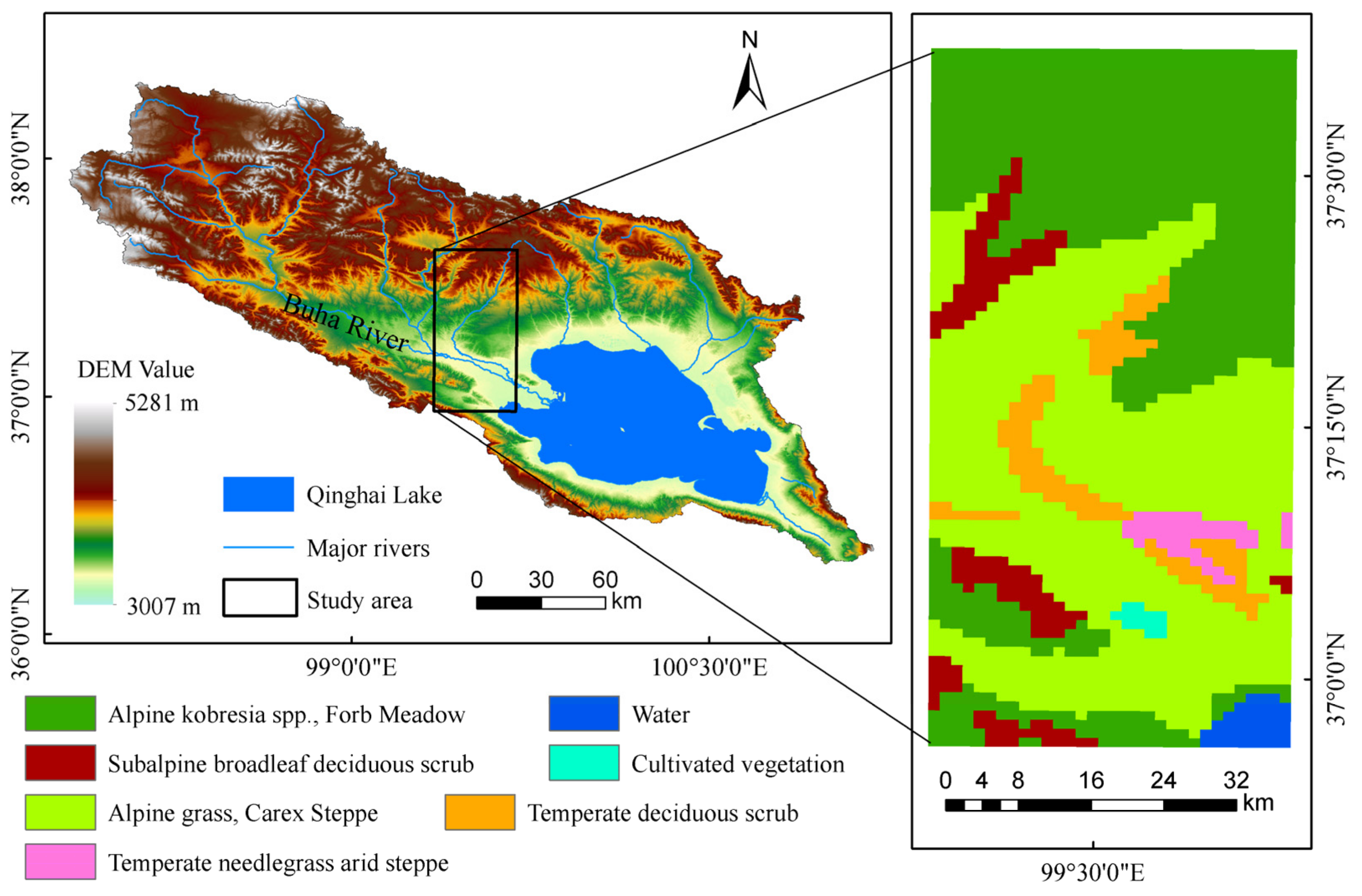
2.1. Study Area

The QLB lies northeast of the QTP and is surrounded by mountains on three sides. Spanning an area of 29,660 km2, this basin is vital in preventing the Qaidam Desert from expanding inland. The altitude of the basin is between 3007 and 5281 m, gradually declining from the northwest to the southeast (Figure 1). The lowest altitude occurs around Qinghai Lake in the southeast, which represents China’s largest inland saltwater lake on the plateau. This lake is located at an altitude of 3196 m and covers a water surface area of 4495 km2 [23]. The Buha River stands as the longest and greatest among over 40 rivers that feed into Qinghai Lake, contributing nearly half of the entire runoff. Moreover, the majority of these rivers are intermittent [24].
The selected study area is located northwest of Qinghai Lake and features rolling terrain with elevations varying from 3162 m to 4287 m. It spans approximately 2300 km2 and lies between 36°56′16″–37°37′01″N and 99°20′37″–99°41′39″E. The annual average temperature falls between −5 and 2 °C, with an average yearly precipitation of 450 mm. The Buha River courses through the southern region, eventually flowing into Qinghai Lake. The selected region is an area covering the major vegetation types in the QLB, where Alpine grass, Carex Steppe (accounting for 45.2%) and Alpine kobresia spp., Forb Meadow (accounting for 39.1%) are widely distributed [25]. The remaining region consists of shrubs and water bodies (Figure 1). Pastoralism is the main industry, with a combination of agriculture, mainly involving yaks and sheep grazing.

2.2. Materials

A total of 88 Landsat-5 Thematic Mapper (TM) and Landsat-8 Operational Land Imager (OLI) views taken in 2001, 2005, 2009, 2011, 2014, 2016, 2019, 2020, and 2022 were retrieved from the USGS archives (https://earthexplorer.usgs.gov/, accessed on 30 March 2023) due to their lower cloud coverage. The Landsat images captured the vegetation growth period spanning from May to October in the study area.
The reflectance data in the red and near-infrared bands of the daily MOD09GQ product and 8-day composited MOD09Q1 product, both of which offer a spatial resolution of 250 m, were retrieved from the NASA data archive (https://ladsweb.modaps.eosdis.nasa.gov/, accessed on 30 March 2023). The MOD09GQ data spanned from 1 May to 10 October (day of year (DOY) from 121 to 283) in the above stated 9 years, for a total of 1467 tiles, while the MOD09Q1 data spanned from 1 May to 8 October (DOY from 121 to 281) in the same years, totaling 189 tiles.
The 1:1 million Chinese vegetation map released by the Resource and Environmental Science and Data Center (http://www.resdc.cn/, accessed on 30 September 2022) was used to provide an overview of the spatial distribution of vegetation in the study area. The digital elevation model was constructed from the publicly accessible online repository of the geospatial data cloud (http://www.gscloud.cn/, accessed on 30 September 2022). The acquired dataset was ASTER GDEM Version 3 in GeoTIFF format with a resolution of 30 m.

3. Methods

3.1. Data Preprocessing

All Landsat images were from Collection 2 Level-1; L1TP are top-of-atmosphere reflectance data that have been radiometrically and geometrically corrected and precision terrain processed. The FLAASH atmospheric correction tool provided by ENVI 5.6 software [26] was then applied to all the images to compensate for atmospheric effects.
To ensure the data quality for subsequent analysis, we used the Cloud Mask Using Fmask Algorithm (version 3.2) to identify and exclude pixels affected by clouds and snow cover [27,28]. Landsat NDVIs were then derived from the reflectance of the near-infrared and red bands.
In addition, we used the MODIS Reprojection Tool (MRT) to convert the MODIS reflectance products into the GeoTIFF format and reprojected them to the WGS84/UTM coordinate system. Then, we calculated the MODIS NDVI values from the near-infrared and red bands and obtained the MODIS daily and 8-day synthetic NDVI time series. The ASTER GDEM 30 m elevation and vegetation map data were also reprojected to the WGS84/UTM coordinate system. Finally, all datasets were extracted based on the extent of the study area.

3.2. Landsat NDVI Time Series Reconstruction

Three procedures were needed for Landsat NDVI time series reconstruction and Landsat annual maximum NDVI derivation. First, the MOD09GQ data should minimize cloud contamination through noise reduction. Second, the existing Landsat and MOD09GQ data were fused to obtain additional intra-annual Landsat simulated NDVIs. Finally, a single-peaked symmetric logistic curve (S-logistic) was applied to fit the vegetation growth process in each pixel and extract the annual maximum NDVI value.

3.2.1. Denoising of MODIS Daily NDVI

Despite filtering using the MOD09GQ product’s quality flag, subpixel cloud contamination still occurred in a large amount of vegetation index (VI) data [29]. In contrast, there was less cloud contamination in the generated composite product (MOD09Q1) when using one of the collected values from the 8-day periods [30]; however, uncertainty inevitably arises in terms of time, and the time interval between two consecutive observations can reach a time error of 0–15 days [31,32], during which subtle short-term vegetation change information will be lost [32,33,34].
To monitor rapid vegetation change events, previous studies have suggested the use of daily VI time series [33,35]. Before using the daily NDVI for fusion, we performed pixel-by-pixel denoising of the daily NDVI using the DAVIR-MUTCOP method [36]. This method combines the accurate date of daily MOD09GQ NDVI and the high quality of composite MOD09Q1 NDVI to screen out more high-quality daily NDVI, which are interpolated to generate the daily MODIS NDVI. For a more detailed description, refer to Zeng [36]. The denoised daily NDVI was then spatially resampled to a 30 m resolution using the bicubic interpolation method, which has been proven to produce smoother results with reduced interpolation distortions [37]. The resampled results were subsequently used for spatiotemporal fusion.
The date when the vegetation growth in each pixel reached the maximum value (Maxday) was also obtained by comparing the reconstructed MODIS daily NDVI. The Maxday was used as the initial parameter for subsequent S-logistic fitting.

3.2.2. Generating Simulated Landsat NDVI

The process of using the corresponding MODIS data to generate simulated Landsat NDVI data based on the ESTARFM is as follows.
If a pair of Landsat and MODIS images are obtained at t m and another MODIS image is obtained at t p , then the prediction pixel values in the center of the Landsat window at t p are:
F x w / 2 , y w / 2 , t p = F x w / 2 , y w / 2 , t m + i = 1 N W i × V i × C x i , y i , t p C x i , y i , t m
where F denotes the Landsat image, t m denotes the reference image acquisition date, C denotes the MODIS image, W denotes the weight, V denotes the conversion factor, ( x w / 2 , y w / 2 ) is the position of the window center pixel, w denotes the window size, N denotes the number of similar pixels, and ( x i , y i ) is the position of the ith similar pixel.
We select two pairs of Landsat and MODIS reference images acquired at different dates and then calculate the center pixel value of the Landsat image for a given prediction date t p based on the above formula. The two prediction results are weighted combinations to produce the final window center pixel value in the predicted image:
F x w / 2 , y w / 2 , t p = T m × F m x w / 2 , y w / 2 , t m + T n × F n x w / 2 , y w / 2 , t n
where F m x w / 2 , y w / 2 , t m and F n x w / 2 , y w / 2 , t n denote the values of the target date t p predicted from the values at the reference dates t m and t n , respectively, and T m and T n denote the temporal weights.
Zhu confirmed that the accuracy of the predicted Landsat image values is affected by the time interval between the reference and predicted images as well as by the inter-image correlation between Landsat and MODIS, but there is no specific index for determining how to select the optimal reference date image [38]. In our study, we used the phase difference parameter proposed by Dong [39] as the selection strategy to improve the prediction result accuracy. For convenience, we named the reference date before the prediction date the “left” reference date and the reference date after the prediction date the “right” reference date. The spatiotemporal correlation parameter P is expressed as follows:
P = R 1 D 1 + R 2 D 2
where R 1 and R 2 denote the correlation between the MODIS image acquired at the predicted date and the MODIS image at the left or the right reference date, respectively; D 1 and D 2 denote the DOY interval between the predicted date and the left or the right reference date, respectively. To improve the availability of the fusion results, four fusion rules are proposed in our study as follows.
  • At most, each Landsat image in the time series should participate in the fusion once.
  • The Landsat images used in the fusion should meet the conditions that the proportion of clear pixels in the image after Fmask 3.2 detection is more than 85%.
  • The predicted image time should be between the left and right reference image dates.
  • Combined with the MOD09GQ NDVI data, the spatiotemporal correlation parameter showed p > 0.1.
We fused only reference images that met the above four fusion rules. The information of the reference and predicted target images participating in the fusion each year is shown in Table 1.

3.2.3. S-Logistic Model Fitting

Sprouting in early spring and peaking in summer is a typical pattern of the natural growth process of vegetation. Logistic models can simulate this growth pattern and are extensively employed in monitoring regional and global vegetation phenology [40,41,42,43]. In our study area, an S-logistic model, improved from the four-parameter logistic model proposed by Zhang [15], was applied to fit the Landsat NDVI growth curve. Compared with other fitting models, the S-logistic model depicts the whole growth and decline process of vegetation within a year with a single-peaked curve [44]. The S-logistic model is described below.
N D V I t = d 1 + e a t b 2 + c + f
where t is the Landsat image date, as well as the date for the predicted target image, and N D V I t is the fitted NDVI at date t . The shape of the fitted curve is controlled by the nonlinear parameters a , b, and c, where b determines the time at which the fitted curve reaches its peak, a, c determines the inflection points and its derivative on the left and right sides of the fitted curve, d is the growth amplitude and f is the minimum NDVI value in winter.
Based on the available NDVIs and dates, the five parameters in Equation (4) were assigned initial values according to the nonlinear least squares fitting solution. Importantly, the regression parameters of the S-logistic model were not manually set based on our experience, but were estimated through iterative optimization using the Levenberg–Marquardt algorithm [45]. This optimization process involved iteratively fitting the model to time series data until the criterion of minimizing the sum of squared residuals was met. When the S-logistic model parameters were determined and the NDVI curve was reconstructed, Maxday was brought into Equation (4) to find the NDVI maximum within the year.

3.3. Evaluation of Reconstruction Method Accuracy

According to the reconstruction curve (Equation (4)), input the DOY of the reference date to calculate the reconstructed NDVI of each pixel and generate the reconstructed series. The RMSE between the reconstructed and reference series on each pixel is calculated as follows:
R M S E = t = 1 s ( N D V I r e f ( t ) N D V I r e c ( t ) ) 2 s
where s is the number of reference Landsat NDVI images in a year, N D V I r e f ( t ) represents the NDVI value of the tth reference series, N D V I r e c ( t ) is the NDVI value of the tth reconstructed series; the smaller the RMSE, the better the performance of the reconstruction method.

3.4. Trend Analysis

One-dimensional linear regression analysis was conducted on the NDVI, with time serving as the independent variable. The regression coefficient ( θ s l o p e ) represents the direction and magnitude of changes in the NDVI time series [46]. It can be calculated as:
θ s l o p e = n i = 1 n i N D V I i i = 1 n i i = 1 n N D V I i n i = 1 n i 2 i = 1 n i 2
where n is the number of study years (n = 9 in this study), N D V I i denotes the NDVI in the ith year, and θ s l o p e is the slope of the linear regression. If θ s l o p e was positive, the NDVI showed an increasing trend during the study period; if θ s l o p e was negative, it was decreasing.
The coefficient of variation (CV) characterizes the degree of dispersion of the time series and measures the degree of fluctuation of the NDVI over time [47]. The CV is calculated at the pixel scale as follows:
C V = 1 n 1 i = 1 n N D V I i N D V I ¯ 2 N D V I ¯
where N D V I ¯ is the mean NDVI of the n years. The larger the CV, the greater the volatility and dispersion of the data, while the opposite is more stable.

4. Results

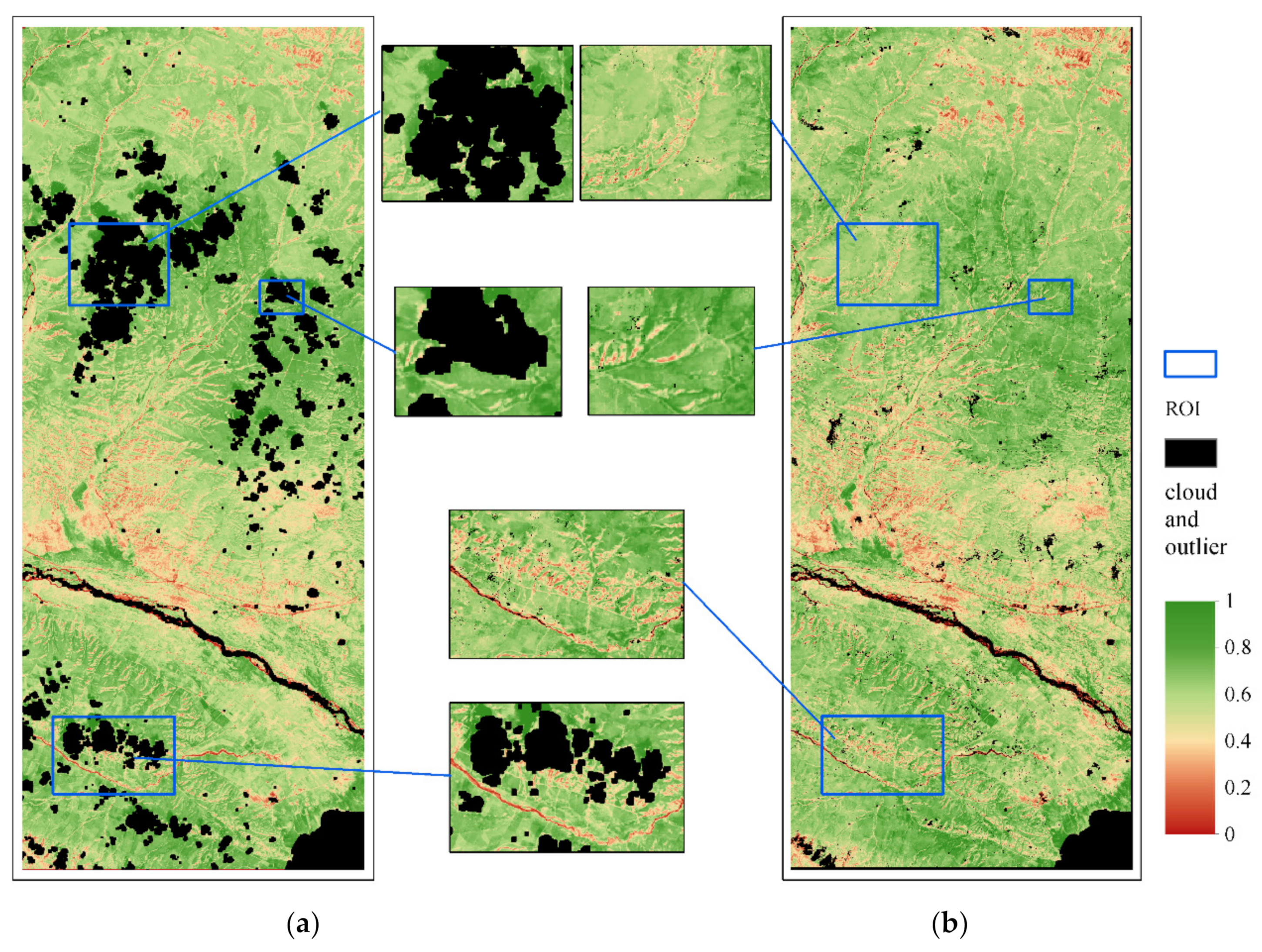
4.1. Validation of the Reconstructed Landsat NDVI

Figure 2 shows the Landsat reference NDVI image acquired on 8 September 2022, which contains numerous pixels affected by cloud cover and the NDVI image processed by our reconstruction algorithm. The overall RMSE between the two images for the cloud-free pixels was 0.077. The reconstructed NDVI image also showed that most of the pixels in the cloud areas were recovered and spatially matched the adjacent pixels.
The 2022 Landsat NDVI reference images were used to evaluate the reconstruction model fitting performance, where n = 8. We counted the number of pixels with an RMSE not exceeding 0.1 as 91.8%. An RMSE greater than 0.1 is mainly distributed in the cloud shadow portion (see Figure 3) because the cloud mask processed with the Calculate Cloud Mask Using Fmask tool in ENVI 5.6 is a binary image where cloud pixels have values of 0 and non-cloud pixels have values of 1 (Calculate Cloud Mask Using Fmask), and the cloud shadow portion is not detected. The effectiveness of the fitted model depends largely on whether it is consistent with the vegetation growth season trajectory [48]. In general, the photosynthetic response of herbaceous plants fluctuates more rapidly within a cycle in response to seasonal climate change; therefore, short-term plateau NDVI curves are more common in grassland ecosystems [49]. Therefore, the S-logistic model is suitable for the NDVI reconstruction of alpine grasslands in the study area, and its NDVI temporal profile is similar to the experimental research results of Liu [48] and Jiang [50].

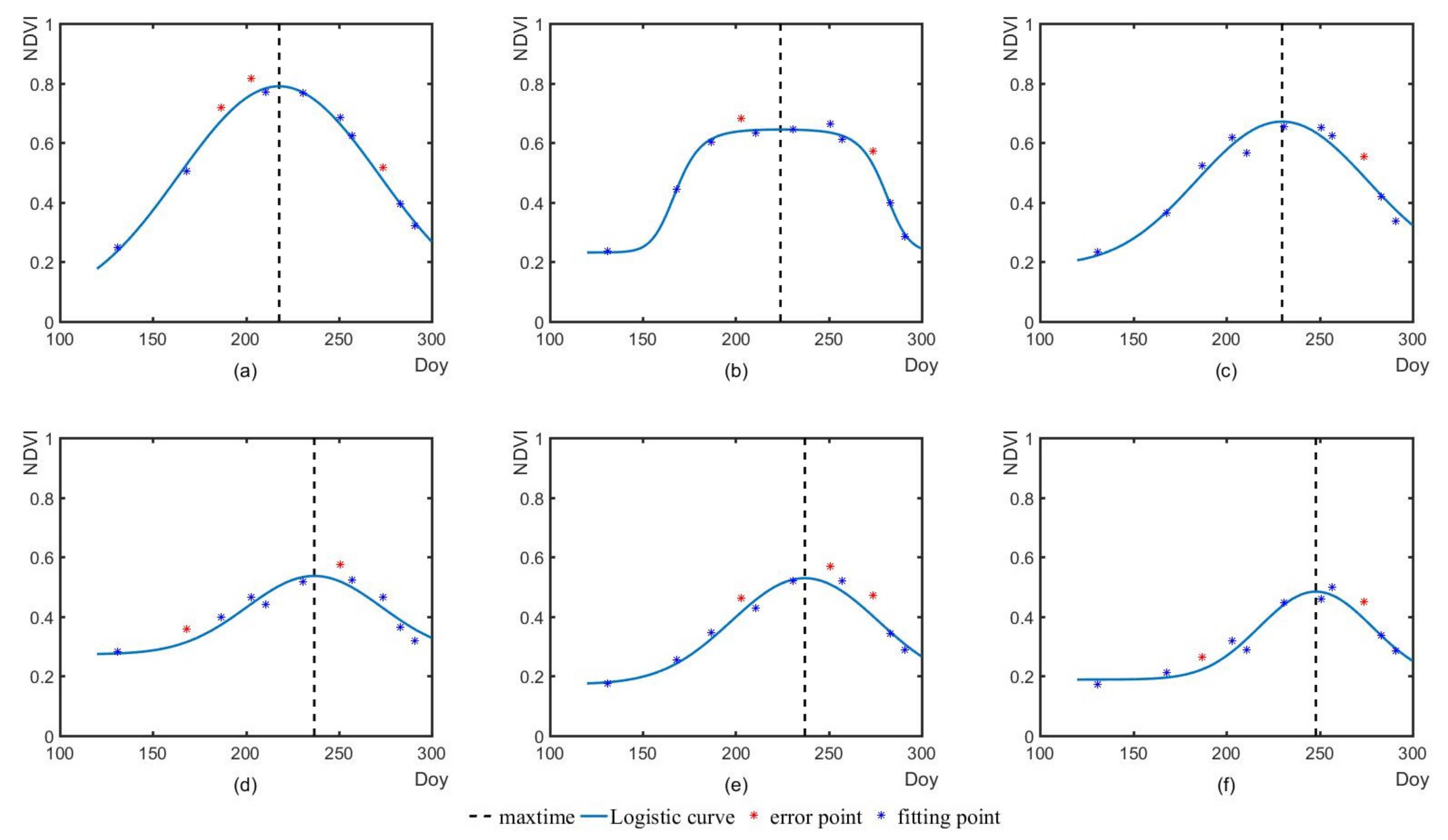
4.2. Vegetation Growth Fitting under Different Coverage Types

To analyze the seasonal characteristics of the Landsat NDVI curves within typical vegetation areas, we randomly selected six pixels for different vegetation types, and Figure 4 shows the NDVI curves of various types of vegetation during the growth period. It is obvious that different types reached their peak growth at different dates, as did the maximum NDVI value.
Although phenological metrics describing the start, end, and length of vegetation growth have been extensively studied, the date when the NDVI reaches a maximum that corresponds to peak photosynthesis has not been well-explored. This maximum reflects the turning point of photosynthetic dynamics from the greening stage to the senescence stage, affecting livestock habitat and forage [51]. We analyzed the spatial distributions and frequency distribution of the Maxday (Figure 5) and maximum NDVI values in 2022 and found the following:
The vegetation (mainly Alpine grass, Carex Steppe) near the banks of the Buha River generally grew at a peak of around 231, and the maximum NDVI value generally reached only approximately 0.6, while the vegetation on the northern and southern edges of the study area (Alpine kobresia spp., Forb Meadow) reached its peak earlier, generally around 213, and the maximum NDVI could reach close to 0.8. The Maxday is related to the vegetation type, and the mean values of Maxday for the different vegetation types were calculated separately, as shown in Table 2:

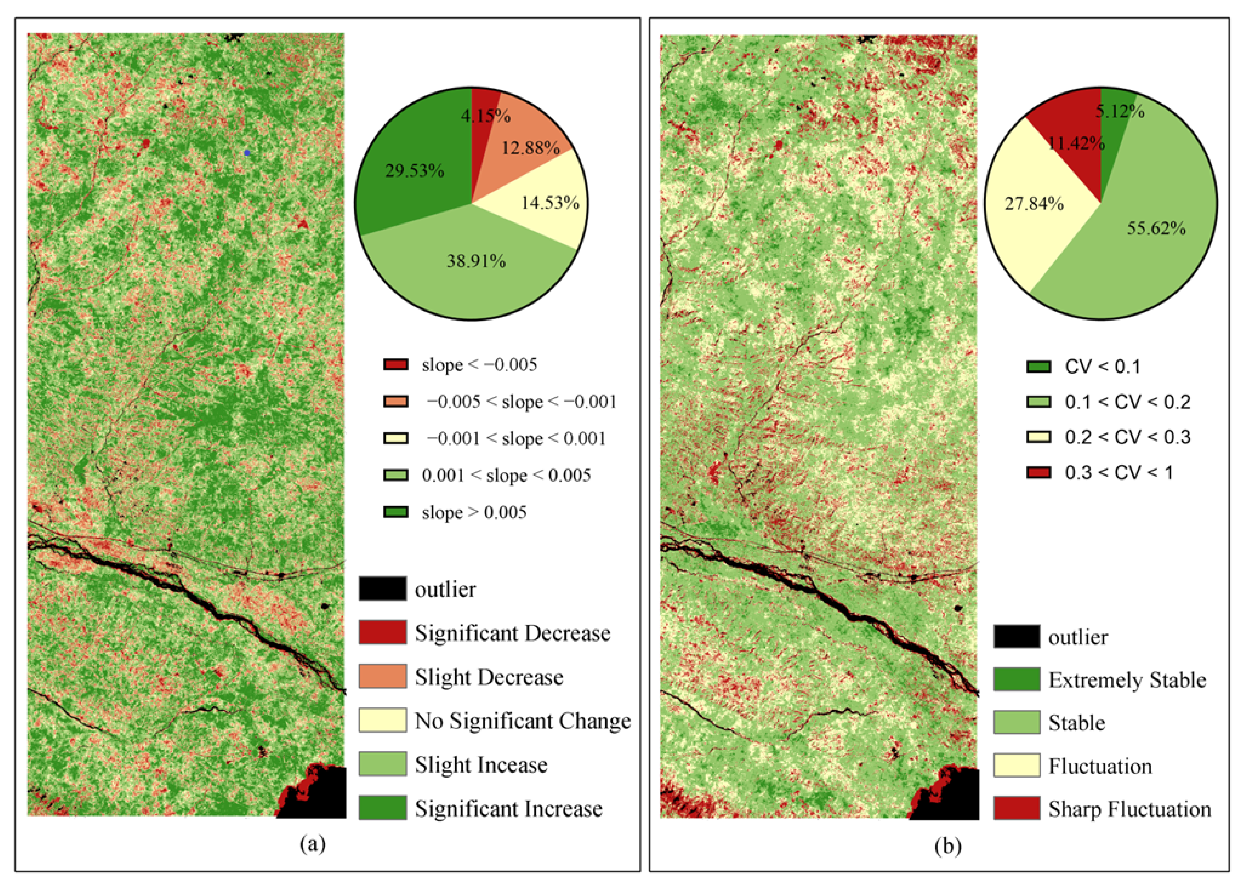
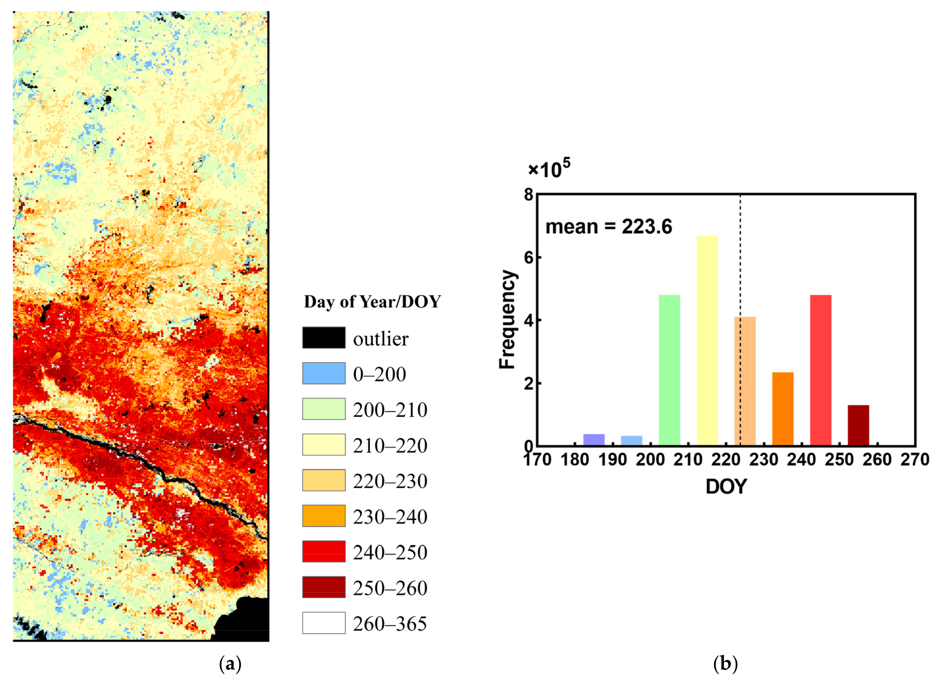
4.3. Spatial and Temporal Patterns of Landsat NDVI Annual Maxima

Figure 6 shows the spatial distribution of the NDVI maxima from 2001 to 2022, where the black regions are non-vegetated areas with an NDVI less than 0, anomalous areas with an NDVI exceeding 1, or areas where the NDVI cannot be reconstructed because of insufficient Landsat true NDVIs.
In comparison, the overall vegetation cover in 2005, 2014, and 2020 was greater than that in other years. The NDVI maxima generally showed high spatial characteristics in the north and south, with values ranging from 0.6 to 0.8, while they were low in the central valley, with values ranging from 0.4 to 0.6.
According to our fieldwork, there are two reasons for the observed spatial differences. The first is the topography; the central part falls within the Buha River alluvial plains, which is used for various human activities such as railroads, highways, settlements, and pastoral areas. In contrast, the northern and southern sides are mainly mountainous, with fewer human dwellings and less intensive grazing. The other reason is related to the type of vegetation present; the mountains on both sides primarily consist of Kobresia pygmaea meadows, which are characterized by the dense growth of small, perennial herbaceous plants thriving in cold, high-altitude areas [52]. The central part of the vegetation is mostly Stipa purpurea steppe, whose leaves are typically linear and relatively slender and often reach lengths of 10–20 cm. Its flowers are purple or pale purple in color and tend to grow at the top of the plant, forming clustered inflorescences [53].
The multiyear average maximum NDVI was 0.623, but the spatial vertical zonation varied significantly [54]. Alpine kobresia spp., Forb Meadow is located on the north and south, and its multiyear average growing season maximum can reach 0.663. Subalpine broadleaf deciduous Scrub was the next highest at 0.652. The values for Alpine grass, Carex Steppe and Cultivated vegetation could reach approximately 0.590, while that for Temperate deciduous scrub was 0.551, and that for Temperate needlegrass arid steppe had the lowest maximum value of 0.521. The average NDVI during the study period reflects the grass biomass capacity for different vegetation.
The spatial distribution of the NDVI intra-annual maximum variation trends from 2001 to 2022 is shown in Figure 7a. The overall trend showed an increasing trend, with an average of 0.0028 per year. Approximately 68% of the area exhibited either a significant increase ( θ s l o p e > 0.005) or a slight increase (0.001 < θ s l o p e < 0.005). The trend of the intra-annual maximum NDVI decreased mostly for Alpine kobresia spp., Forb Meadow and Temperate deciduous scrub and was characterized as patches.
Figure 7b shows the CV of the NDVI intra-annual maxima from 2001 to 2022. The study area’s variability was mainly stable, and nearly 40% of the area was distributed as patches in fluctuating or sharply fluctuating states. In particular, the areas in a sharp fluctuation state were also concentrated in Alpine kobresia spp., Forb Meadow in the southwest and northeast, and Temperate deciduous scrub on banks of the river valley.

5. Discussion

5.1. Advantages and Limits of Reconstructed Landsat NDVI

This study aimed to address the limitations of the current NDVI time series in monitoring grassland degradation in fragmented landscapes. Two limitations are the insufficient spatial resolution of the NDVI series and the impact of intra-annual vegetation phenology. To tackle these issues, this study explored a method for reconstructing a Landsat NDVI time series and deriving the annual maximum NDVI. This method involved using higher frequency MODIS NDVI data and combining ESTARFM and the S-logistic model.
The S-logistic model has fewer parameters and requires fewer NDVIs to simulate vegetation growth, which is essential in the QTP where clouds and rainfall occur frequently during the vegetation growing season. The ESTARFM can fill in the gaps in the existing Landsat data, but it relies on the linear principle when predicting new images while vegetation grows nonlinearly; a typical example is at the transitional stage including the maximum NDVI. We must propose four fusion rules to achieve a balance between meeting the requirements of S-logistic fitting and minimizing the errors. We examined the reconstructed results in 2022 and found that 91.8% of the RMSEs fell within 0.1 compared with the original reference images, as shown in Figure 2.
Generally, the photosynthetic response of herbaceous plants fluctuates rapidly with seasonal changes within a growth cycle [49], and in grassland ecosystems, photosynthesis rarely exhibits long-term peaks in the growth phase. After reaching its maximum, it also rapidly enters the senescence phase [48]. Alpine grass commonly experiences a singular vegetation peak during the summer growing season, which aligns well with the characteristics of an S-logistic curve. We used Maxday, a derivative of the MOD09GQ and MOD09Q1 series cross-correction, as the initial value of parameter b during S-logistic iteration. MODIS data are considered to have minimal influence from clouds, viewing angles, and atmospheric aerosols [55,56], so using the Maxday derived from MODIS data not only provides more accurate peak dates, but also saves time in the S-logistic fitting iterations. Other parameters are not needed beforehand because the prediction function can be iteratively adjusted through the existing optimization rule for the Levenberg–Marquardt algorithm until the parameters automatically satisfy the minimum RMSE, which yields a more flexible and stable estimation for different vegetation types.
Dong developed a 30-m annual maximum NDVI dataset for China from 2000 to 2020 [57] using Savitzky–Golay filtering to fill gaps and the generalized additive model to smooth data [49]. The dataset was released by the National Ecosystem Science Data Center (http://www.nesdc.org.cn/, accessed on 30 June 2023). We calculated the RMSE between the two datasets and the actual values in the study area. Landsat NDVI on August 9th, 2020 (DOY = 222) was used as the actual or true values to validate the accuracy of both datasets. First, we extracted pixel locations corresponding to Maxday when DOY = 222 and identified 153,146 pixel locations. Then, we took the Landsat NDVI values at these locations on August 9th as ground truths and calculated the RMSE between our results and the ground truths as well as the RMSE between the national products and the ground truths. The calculated values were 0.066 and 0.190, respectively. Therefore, our data achieved higher accuracy within the study area.
However, due to the severity of the missing Landsat data resulting from cloud cover or low-quality MODIS data during the study period, there were still a few zones where the NDVI could not be reconstructed successfully, as shown by the outlier values in Figure 6. In addition, as the satellite equipped with the MODIS sensor was launched in 2000, the Landsat NDVI could not be reconstructed before 2000 by ESTARFM and S-logistic fitting. On a larger scale, many pixels affected by clouds will inevitably appear. In light of the data missing problem caused by cloud coverage, some methods have been proposed to remove the effects of thick clouds such as the modified neighborhood similar pixel interpolator (MNSPI) [58], which uses similar pixels in spatial and temporal neighborhoods to interpolate thick cloud pixels, autoregression to remove clouds (ARRC) [59], an algorithm to weigh the autocorrelation of long-term data and distance similarity of short-term data, spatio-temporal tensor [60], and deep learning techniques [61].

5.2. Reasons for Spatial Characteristics and Variations in Vegetation NDVI

Our results showed that earlier vegetation growth maximum dates were accompanied by higher NDVI maxima. For example, for Alpine kobresia spp., Forb Meadow, the maximum NDVI values appeared at the beginning of August, while in areas with smaller NDVI maxima such as Alpine grass, Carex Steppe, the growth maximum dates appeared in mid-August. Our findings are consistent with prior research conducted using low-resolution remote sensing images. For example, Duan used the vegetation index derived from MOD13A2 with a resolution of 1 km every16 days [62], and Wang used MOD09A1 captured at 500 m intervals occurring every 8 days [63]. Their results showed that alpine meadows have greater maximum NDVI values and earlier maxima dates than alpine steppes throughout the QTP, but they studied only the two most widely distributed vegetation types (i.e., meadows and steppes). In addition, our study provided more refined results or insights at a smaller scale such as a magnifier and involved more vegetation such as shrubs and plantations.
On the QTP, greening trends have been observed in many studies. Liu used the MVC method to construct an 8 km NDVImax time series from 1981 to 2019 and concluded that the QTP was generally greening, with only localized degradation from 2000 to 2019 [6]. Chen also reached similar conclusions based on the MOD13A2 NDVI dataset [7]. However, large-scale studies are often inconsistent with those at small scales, as grassland degradation generally starts in small plots and then extends into patches. Our study did find small degraded patches in areas of overall greening, and it is even more important that we focus on monitoring these small patches of grass that may expand the extent of degradation.
Previous studies have shown that climate factors significantly impact the NDVI variability in alpine vegetation [64]. Lehnert analyzed trends in grassland cover using MCD43A4 and explored the interactions among vegetation dynamics, climate shifts, and human influences on the QTP, concluding that large-scale alterations in grassland cover on the QTP stemmed more from climate variability than overstocking [65]. Other studies affirmed a correlation between vegetation growth in the northeastern QTP and spring temperature and summer precipitation [66]. Alpine meadows are the most sensitive and complex in their response to climate shifts [7,67], and climate warming will promote their rapid growth. Moreover, the melting of ice and snow caused by high temperatures adversely affects the growth of shallow-rooted plants [68]. Another result of a warming climate is the degradation of frozen soil [69], causing a decline in the water table, soil desiccation, and the subsequent degradation of alpine meadows [70,71].
Apart from the greater influence of climate on alpine meadow vegetation, the proliferation of wildlife and anthropogenic overgrazing can also lead to vegetation degradation. According to our field work, guided by the results of the NDVI slope and CV spatial distribution, localized degradation in the study area should be attributed to a combination of permafrost degradation, overgrazing, and rodent infestation. The number of sheep equivalents in Gangcha County significantly increased, rising from 1,587,800 in 2000 to 1,891,600 in 2017, representing a 19% increase [72], which puts great pressure on the grassland, especially in the widely distributed alpine meadow area where Kobresia pygmaea is a high-quality forage grass. However, the explosive increase in plateau pikas has severely impacted the local grassland in the study area. We conducted field work at some of the sites in 2023 where the NDVI slope was declining and changing dramatically. Figure 8, Figure 9 and Figure 10 show one of the degraded sites, which is in seasonally frozen soil with severe rodent infestation. An increase in the frequency of the freeze–thaw cycle hastened nutrient depletion and reduced the soil’s ability to retain water [73], ultimately resulting in the degradation of alpine meadows. Without proper management, the eventual outcome will be the development of black soil conditions, which pertains to the significant deterioration of grasslands caused by factors such as excessive grazing, rodent infestation, cycles of freezing and thawing as well as wind or water erosion. These factors lead to sparse vegetation and diminished land cover [74].
It is crucial to prioritize the monitoring of soil properties in alpine meadows as these properties significantly contribute to stabilizing and improving the ecosystem services offered by alpine grasslands against climate warming. The study’s discoveries can lay a foundation for local political institutions to safeguard grassland ecosystems and maintain an ecological balance.

6. Conclusions

The QLB lies on the northeastern Tibetan Plateau and serves as a crucial barrier in preventing the expansion of the Qaidam Desert into inland China. Monitoring and analyzing alterations in the region’s vegetation are relevant for gaining insights into climate change responses and formulating sustainable ecological conservation policies. In this study, we addressed the critical issue of the low resolution of NDVI time series data and improved the data sources for grassland monitoring. In addition, we conducted an analysis of the distribution of the annual maximum NDVI from 2001 to 2022, revealing its spatial pattern and interannual variability. The following conclusions were drawn:
  • By leveraging the unique spatiotemporal advantages of MODIS NDVI and Landsat NDVI data, we successfully derived the maximum NDVI for the whole year independent of the season at high resolution. The reconstruction results showed higher accuracy than those of the existing dataset. Our study provides more refined reconstruction results for the spatial characterization and variability of the NDVI at a fragmented landscape scale.
  • Similarly, the annual maximum NDVI from 2001 to 2022 exhibited spatial vertical distribution differences, with higher values ranging from 0.6 to 0.8 in the northern and the southern regions, and lower values from 0.4 to 0.6 in the middle region. The maximum NDVI in Alpine kobresia spp., Forb Meadow was much higher than the average, and that in Temperate needlegrass arid steppe was significantly lower than the average. Furthermore, the earlier vegetation growth maximum dates were accompanied by greater NDVI maxima.
  • From 2001 to 2022, the annual NDVI maximum value increased slightly, with a growth rate of 0.0028 per year. The annual maximum NDVI showed a decreasing trend mainly for Alpine kobresia spp., Forb Meadow and Temperate deciduous scrub. Nearly 40% of the area was distributed as patches in fluctuating or sharply fluctuating states. In particular, the areas in a sharp fluctuation state are also concentrated in Alpine kobresia spp., Forb Meadow in the southwest and northeast, and Temperate deciduous scrub on both sides of the river valley.
However, with ongoing climate warming, the soil moisture and nutrients in alpine meadows affected by permafrost degradation, rodent infestation, and overgrazing may face degradation, and the root growth patterns of alpine meadows could shift, potentially resulting in a decrease in grassland ecosystem services. To avoid serious consequences, there is an urgent need to implement effective measures to restore degraded alpine meadows, aiming to attain sustainable rejuvenation goals.

Author Contributions

Conceptualization, F.L. and G.W.; Methodology, M.L. and F.L.; Software, M.L.; Validation, M.L., A.S. and Y.W.; Formal analysis, G.W.; Investigation, M.L., A.S. and Y.W.; Resources, G.W.; Data curation, A.S.; Writing—original draft preparation, M.L.; Writing—review and editing, G.W.; Visualization, M.L.; Supervision, G.W.; Project administration, G.W.; Funding acquisition, S.L. All authors have read and agreed to the published version of the manuscript.

Funding

This research was funded by the Strategic Priority Research Program of the Chinese Academy of Sciences, grant number XDA20100103, and the Applied Fundamental Research Foundation of Qinghai Province in China, grant number 2017-ZJ-743.

Data Availability Statement

The raw data supporting the conclusions of this article will be made available by the authors on request.

Acknowledgments

We sincerely thank the Foundation for its support of our field work. We would also like to thank the anonymous reviewers for their constructive comments on the manuscript.

Conflicts of Interest

The authors declare no conflicts of interest.

References

  1. Zhang, H.; Zhao, Y.; Zhu, J.K. Thriving under Stress: How Plants Balance Growth and the Stress Response. Dev. Cell 2020, 55, 529–543. [Google Scholar] [CrossRef] [PubMed]
  2. Camacho-De Coca, F.; García-Haro, F.; Gilabert, M.; Meliá, J. Vegetation cover seasonal changes assessment from TM imagery in a semi-arid landscape. Int. J. Remote Sens. 2004, 25, 3451–3476. [Google Scholar] [CrossRef]
  3. Zeng, L.; Wardlow, B.D.; Xiang, D.; Hu, S.; Li, D. A review of vegetation phenological metrics extraction using time-series, multispectral satellite data. Remote Sens. Environ. 2020, 237, 111511. [Google Scholar] [CrossRef]
  4. Busetto, L.; Meroni, M.; Colombo, R. Combining medium and coarse spatial resolution satellite data to improve the estimation of sub-pixel NDVI time series. Remote Sens. Environ. 2008, 112, 118–131. [Google Scholar] [CrossRef]
  5. Jin, X.; Liu, J.; Wang, S.; Xia, W. Vegetation dynamics and their response to groundwater and climate variables in Qaidam Basin, China. Int. J. Remote Sens. 2016, 37, 710–728. [Google Scholar] [CrossRef]
  6. Liu, E.; Xiao, X.; Shao, H.; Yang, X.; Zhang, Y.; Yang, Y. Climate Change and Livestock Management Drove Extensive Vegetation Recovery in the Qinghai-Tibet Plateau. Remote Sens. 2021, 13, 4808. [Google Scholar] [CrossRef]
  7. Chen, J.; Yan, F.; Lu, Q. Spatiotemporal Variation of Vegetation on the Qinghai–Tibet Plateau and the Influence of Climatic Factors and Human Activities on Vegetation Trend (2000–2019). Remote Sens. 2020, 12, 3150. [Google Scholar] [CrossRef]
  8. Wang, X.; Yi, S.; Wu, Q.; Yang, K.; Ding, Y. The role of permafrost and soil water in distribution of alpine grassland and its NDVI dynamics on the Qinghai-Tibetan Plateau. Glob. Planet. Chang. 2016, 147, 40–53. [Google Scholar] [CrossRef]
  9. Li, L.; Fassnacht, F.E.; Storch, I.; Bürgi, M. Land-use regime shift triggered the recent degradation of alpine pastures in Nyanpo Yutse of the eastern Qinghai-Tibetan Plateau. Landsc. Ecol. 2017, 32, 2187–2203. [Google Scholar] [CrossRef]
  10. Fassnacht, F.E.; Schiller, C.; Kattenborn, T.; Zhao, X.; Qu, J. A Landsat-based vegetation trend product of the Tibetan Plateau for the time-period 1990–2018. Sci. Data 2019, 6, 78. [Google Scholar] [CrossRef]
  11. Lhermitte, S.; Verbesselt, J.; Verstraeten, W.W.; Veraverbeke, S.; Coppin, P. Assessing intra-annual vegetation regrowth after fire using the pixel based regeneration index. ISPRS J. Photogramm. Remote Sens. 2011, 66, 17–27. [Google Scholar] [CrossRef]
  12. Wang, Z.; Cao, S.; Cao, G.; Lan, Y. Effects of vegetation phenology on vegetation productivity in the Qinghai Lake Basin of the Northeastern Qinghai–Tibet Plateau. Arab. J. Geosci. 2021, 14, 1030. [Google Scholar] [CrossRef]
  13. Wulder, M.A.; Loveland, T.R.; Roy, D.P.; Crawford, C.J.; Masek, J.G.; Woodcock, C.E.; Allen, R.G.; Anderson, M.C.; Belward, A.S.; Cohen, W.B.; et al. Current status of Landsat program, science, and applications. Remote Sens. Environ. 2019, 225, 127–147. [Google Scholar] [CrossRef]
  14. Cuomo, V.; Lanfredi, M.; Lasaponara, R.; Macchiato, M.F.; Simoniello, T. Detection of interannual variation of vegetation in middle and southern Italy during 1985-1999 with 1 km NOAA AVHRR NDVI data. J. Geophys. Res. Atmos. 2001, 106, 17863–17876. [Google Scholar] [CrossRef]
  15. Zhang, X.; Friedl, M.A.; Schaaf, C.B.; Strahler, A.H.; Hodges, J.C.F.; Gao, F.; Reed, B.C.; Huete, A. Monitoring vegetation phenology using MODIS. Remote Sens. Environ. 2003, 84, 471–475. [Google Scholar] [CrossRef]
  16. Jonsson, P.; Eklundh, L. Seasonality extraction by function fitting to time-series of satellite sensor data. IEEE Trans. Geosci. Remote Sens. 2002, 40, 1824–1832. [Google Scholar] [CrossRef]
  17. Chen, J.; Jönsson, P.; Tamura, M.; Gu, Z.; Matsushita, B.; Eklundh, L. A simple method for reconstructing a high-quality NDVI time-series data set based on the Savitzky–Golay filter. Remote Sens. Environ. 2004, 91, 332–344. [Google Scholar] [CrossRef]
  18. Viovy, N.; Arino, O.; Belward, A.S. The Best Index Slope Extraction (BISE): A method for reducing noise in NDVI time-series. Int. J. Remote Sens. 1992, 13, 1585–1590. [Google Scholar] [CrossRef]
  19. Menenti, M.; Azzali, S.; Verhoef, W.; Van Swol, R. Mapping agroecological zones and time lag in vegetation growth by means of Fourier analysis of time series of NDVI images. Adv. Space Res. 1993, 13, 233–237. [Google Scholar] [CrossRef]
  20. Cao, R.; Chen, Y.; Shen, M.; Chen, J.; Zhou, J.; Wang, C.; Yang, W. A simple method to improve the quality of NDVI time-series data by integrating spatiotemporal information with the Savitzky-Golay filter. Remote Sens. Environ. 2018, 217, 244–257. [Google Scholar] [CrossRef]
  21. Chen, Y.; Cao, R.; Chen, J.; Liu, L.; Matsushita, B. A practical approach to reconstruct high-quality Landsat NDVI time-series data by gap filling and the Savitzky–Golay filter. ISPRS J. Photogramm. Remote Sens. 2021, 180, 174–190. [Google Scholar] [CrossRef]
  22. Yan, L.; Roy, D.P. Spatially and temporally complete Landsat reflectance time series modelling: The fill-and-fit approach. Remote Sens. Environ. 2020, 241, 111718. [Google Scholar] [CrossRef]
  23. Chen, Q.; Liu, W.; Huang, C. Long-Term 10 m Resolution Water Dynamics of Qinghai Lake and the Driving Factors. Water 2022, 14, 671. [Google Scholar] [CrossRef]
  24. Li, X.Y.; Ma, Y.J.; Xu, H.Y.; Wang, J.H.; Zhang, D.S. Impact of land use and land cover change on environmental degradation in lake Qinghai watershed, northeast Qinghai-Tibet Plateau. Land. Degrad. Dev. 2009, 20, 69–83. [Google Scholar] [CrossRef]
  25. Gui-chen, C.; Min, P. Types and Distribution of Vegetation in Qinghai Lake Region. Chin. J. Plant Ecol. 1993, 17, 71–81. [Google Scholar]
  26. Cooley, T.; Anderson, G.P.; Felde, G.W.; Hoke, M.L.; Ratkowski, A.J.; Chetwynd, J.H.; Gardner, J.A.; Adler-Golden, S.M.; Matthew, M.W.; Berk, A.; et al. FLAASH, a MODTRAN4-based atmospheric correction algorithm, its application and validation. In Proceedings of the IEEE International Geoscience and Remote Sensing Symposium, IEEE International Geoscience and Remote Sensing Symposium, Toronto, ON, Canada, 24–28 June 2002; Volume 1413, pp. 1414–1418. [Google Scholar]
  27. Zhu, Z.; Woodcock, C.E. Object-based cloud and cloud shadow detection in Landsat imagery. Remote Sens. Environ. 2012, 118, 83–94. [Google Scholar] [CrossRef]
  28. Zhu, Z.; Wang, S.; Woodcock, C.E. Improvement and expansion of the Fmask algorithm: Cloud, cloud shadow, and snow detection for Landsats 4-7, 8, and Sentinel 2 images. Remote Sens. Environ. Interdiscip. J. 2015, 159, 269–277. [Google Scholar] [CrossRef]
  29. Motohka, T.; Nasahara, K.N.; Murakami, K.; Nagai, S. Evaluation of Sub-Pixel Cloud Noises on MODIS Daily Spectral Indices Based on in situ Measurements. Remote Sens. 2011, 3, 1644–1662. [Google Scholar] [CrossRef]
  30. Justice, C.O.; Townshend, J.R.G.; Vermote, E.F.; Masuoka, E.; Wolfe, R.E.; Saleous, N.; Roy, D.P.; Morisette, J.T. An overview of MODIS Land data processing and product status. Remote Sens. Environ. 2002, 83, 3–15. [Google Scholar] [CrossRef]
  31. Guindin-Garcia, N.; Gitelson, A.A.; Arkebauer, T.J.; Shanahan, J.; Weiss, A. An evaluation of MODIS 8- and 16-day composite products for monitoring maize green leaf area index. Agric. For. Meteorol. 2012, 161, 15–25. [Google Scholar] [CrossRef]
  32. Wessels, K.J.; Bachoo, A.; Archibald, S. Influence of composite period and date of observation on phenological metrics extracted from MODIS data. In Proceedings of the 33rd International Symposium on Remote Sensing of Environment: Sustaining the Millennium Development Goals, Stresa, Lago Magglore, Italy, 4–8 May 2009. [Google Scholar]
  33. Narasimhan, R.; Stow, D. Daily MODIS products for analyzing early season vegetation dynamics across the North Slope of Alaska. Remote Sens. Environ. 2010, 114, 1251–1262. [Google Scholar] [CrossRef]
  34. McKellip, R.; Ryan, R.E.; Blonski, S.; Prados, D. Crop surveillance demonstration using a near-daily MODIS derived vegetation index time series. In Proceedings of the Third International Workshop on the Analysis of Multitemporal Remote Sensing Images (MultiTemp 2005), Biloxi, MS, USA, 16–18 May 2005. [Google Scholar]
  35. Jin, S.; Sader, S.A. MODIS time-series imagery for forest disturbance detection and quantification of patch size effects. Remote Sens. Environ. 2005, 99, 462–470. [Google Scholar] [CrossRef]
  36. Zeng, L.; Wardlow, B.D.; Hu, S.; Zhang, X.; Wu, W. A Novel Strategy to Reconstruct NDVI Time-Series with High Temporal Resolution from MODIS Multi-Temporal Composite Products. Remote Sens. 2021, 13, 1397. [Google Scholar] [CrossRef]
  37. Keys, R. Cubic convolution interpolation for digital image processing. IEEE Trans. Acoust. Speech Signal Process. 1981, 29, 1153–1160. [Google Scholar] [CrossRef]
  38. Zhu, X.; Cai, F.; Tian, J.; Williams, T. Spatiotemporal Fusion of Multisource Remote Sensing Data: Literature Survey, Taxonomy, Principles, Applications, and Future Directions. Remote Sens. 2018, 10, 527. [Google Scholar] [CrossRef]
  39. Dong, S. Analysis and Improvenment of Spatial-Temporal Fusion Method of Remote Sensing Image Based on Weight Filtering. Master’s Thesis, Shandong University of Science and Technology, Qingdao, China, 2019. [Google Scholar]
  40. Zhang, X.; Friedl, M.A.; Schaaf, C.B. Global vegetation phenology from Moderate Resolution Imaging Spectroradiometer (MODIS): Evaluation of global patterns and comparison with in situ measurements. J. Geophys. Res. Biogeosci. 2006, 111, G4. [Google Scholar] [CrossRef]
  41. Shen, M.; Tang, Y.; Chen, J.; Yang, W. Specification of thermal growing season in temperate China from 1960 to 2009. Clim. Chang. 2012, 114, 783–798. [Google Scholar] [CrossRef]
  42. Zhu, W.; Tian, H.; Xu, X.; Pan, Y.; Chen, G.; Lin, W. Extension of the growing season due to delayed autumn over mid and high latitudes in North America during 1982–2006. Glob. Ecol. Biogeogr. 2012, 21, 260–271. [Google Scholar] [CrossRef]
  43. Cao, R.; Chen, J.; Shen, M.; Tang, Y. An improved logistic method for detecting spring vegetation phenology in grasslands from MODIS EVI time-series data. Agric. For. Meteorol. 2015, 200, 9–20. [Google Scholar] [CrossRef]
  44. Jiang, L.; Shang, S. Comparison of Fitting Curves on the Dynamic of Vegetation Index. J. Irrig. Drain. 2014, 33, 382–384, 403. [Google Scholar]
  45. Madsen, K.; Nielsen, H.B.; Tingleff, O. Methods for Non-Linear Least Squares Problems; Technical University of Denmark: Kongens Lyngby, Denmark, 2004. [Google Scholar]
  46. Bashir, B.; Cao, C.; Naeem, S.; Joharestani, M.Z.; Bo, X.; Afzal, H.; Jamal, K.; Mumtaz, F. Spatio-Temporal Vegetation Dynamic and Persistence under Climatic and Anthropogenic Factors. Remote Sens. 2020, 12, 2612. [Google Scholar] [CrossRef]
  47. Zhao, S.; Zhao, X.; Zhao, J.; Liu, N.; Sun, M.; Mu, B.; Sun, N.; Guo, Y. Grassland Conservation Effectiveness of National Nature Reserves in Northern China. Remote Sens. 2022, 14, 1760. [Google Scholar] [CrossRef]
  48. Liu, R.; Shang, R.; Liu, Y.; Lu, X. Global evaluation of gap-filling approaches for seasonal NDVI with considering vegetation growth trajectory, protection of key point, noise resistance and curve stability. Remote Sens. Environ. 2017, 189, 164–179. [Google Scholar] [CrossRef]
  49. Yang, J.; Dong, J.; Xiao, X.; Dai, J.; Wu, C.; Xia, J.; Zhao, G.; Zhao, M.; Li, Z.; Zhang, Y.; et al. Divergent shifts in peak photosynthesis timing of temperate and alpine grasslands in China. Remote Sens. Environ. 2019, 233, 111395. [Google Scholar] [CrossRef]
  50. Michel, U.; Jiang, J.; Song, J.; Wang, J.; Xiao, Z.; Civco, D.L.; Ehlers, M.; Schulz, K.; Nikolakopoulos, K.G.; Habib, S.; et al. Combine MODIS and HJ-1 CCD NDVI with logistic model to generate high spatial and temporal resolution NDVI data. In Proceedings of the Earth Resources and Environmental Remote Sensing/GIS Applications III, Edinburgh, UK, 24–27 September 2012; pp. 242–250. [Google Scholar]
  51. Gonsamo, A.; Chen, J.M.; Ooi, Y.W. Peak season plant activity shift towards spring is reflected by increasing carbon uptake by extratropical ecosystems. Glob. Chang. Biol. 2018, 24, 2117–2128. [Google Scholar] [CrossRef] [PubMed]
  52. Miehe, G.; Schleuss, P.M.; Seeber, E.; Babel, W.; Biermann, T.; Braendle, M.; Chen, F.; Coners, H.; Foken, T.; Gerken, T.; et al. The Kobresia pygmaea ecosystem of the Tibetan highlands—Origin, functioning and degradation of the world’s largest pastoral alpine ecosystem: Kobresia pastures of Tibet. Sci. Total Environ. 2019, 648, 754–771. [Google Scholar] [CrossRef] [PubMed]
  53. Miehe, G.; Bach, K.; Miehe, S.; Kluge, J.; Yongping, Y.; Duo, L.; Co, S.; Wesche, K. Alpine steppe plant communities of the Tibetan highlands. Appl. Veg. Sci. 2011, 14, 547–560. [Google Scholar] [CrossRef]
  54. Li, X. Grassland type and distribution in Qinghai lake drainage area. Qinghai Prataculture 2009, 18, 20–23+19. [Google Scholar]
  55. Schaaf, C.B.; Gao, F.; Strahler, A.H.; Lucht, W.; Li, X.; Tsang, T.; Strugnell, N.C.; Zhang, X.; Jin, Y.; Muller, J.-P. First operational BRDF, albedo nadir reflectance products from MODIS. Remote Sens. Environ. 2002, 83, 135–148. [Google Scholar] [CrossRef]
  56. Huete, A.; Didan, K.; Miura, T.; Rodriguez, E.P.; Gao, X.; Ferreira, L.G. Overview of the radiometric and biophysical performance of the MODIS vegetation indices. Remote Sens. Environ. 2002, 83, 195–213. [Google Scholar] [CrossRef]
  57. Dong, J.; Zhou, Y.; You, N. 30-Meter Annual Maximum NDVI Dataset in China, 2000–2020; [DS/OL]; National Ecosystem Science Data Center: Beijing, China, 2021; Available online: https://cstr.cn/15732.11.nesdc.ecodb.rs.2021.012 (accessed on 30 March 2023). [CrossRef]
  58. Zhu, X.; Gao, F.; Liu, D.; Chen, J. A Modified Neighborhood Similar Pixel Interpolator Approach for Removing Thick Clouds in Landsat Images. IEEE Geosci. Remote Sens. Lett. 2012, 9, 521–525. [Google Scholar] [CrossRef]
  59. Cao, R.; Chen, Y.; Chen, J.; Zhu, X.; Shen, M. Thick cloud removal in Landsat images based on autoregression of Landsat time-series data. Remote Sens. Environ. 2020, 249, 112001. [Google Scholar] [CrossRef]
  60. Chu, D.; Shen, H.F.; Guan, X.B.; Chen, J.M.; Li, X.H.; Li, J.; Zhang, L.P. Long time-series NDVI reconstruction in cloud-prone regions via spatio-temporal tensor completion. Remote Sens. Environ. 2021, 264, 112632. [Google Scholar] [CrossRef]
  61. Zhang, Q.; Yuan, Q.; Li, J.; Li, Z.; Shen, H.; Zhang, L. Thick cloud and cloud shadow removal in multitemporal imagery using progressively spatio-temporal patch group deep learning. ISPRS J. Photogramm. Remote Sens. 2020, 162, 148–160. [Google Scholar] [CrossRef]
  62. Duan, H.; Xue, X.; Wang, T.; Kang, W.; Liao, J.; Liu, S. Spatial and Temporal Differences in Alpine Meadow, Alpine Steppe and All Vegetation of the Qinghai-Tibetan Plateau and Their Responses to Climate Change. Remote Sens. 2021, 13, 669. [Google Scholar] [CrossRef]
  63. Wang, C.; Guo, H.; Zhang, L.; Liu, S.; Qiu, Y.; Sun, Z. Assessing phenological change and climatic control of alpine grasslands in the Tibetan Plateau with MODIS time series. Int. J. Biometeorol. 2015, 59, 11–23. [Google Scholar] [CrossRef] [PubMed]
  64. Li, L.; Zhang, Y.; Wu, J.; Li, S.; Zhang, B.; Zu, J.; Zhang, H.; Ding, M.; Paudel, B. Increasing sensitivity of alpine grasslands to climate variability along an elevational gradient on the Qinghai-Tibet Plateau. Sci. Total Environ. 2019, 678, 21–29. [Google Scholar] [CrossRef] [PubMed]
  65. Lehnert, L.W.; Wesche, K.; Trachte, K.; Reudenbach, C.; Bendix, J. Climate variability rather than overstocking causes recent large scale cover changes of Tibetan pastures. Sci. Rep. 2016, 6, 24367. [Google Scholar] [CrossRef]
  66. Gao, X.; Huang, X.; Lo, K.; Dang, Q.; Wen, R. Vegetation responses to climate change in the Qilian Mountain Nature Reserve, Northwest China. Glob. Ecol. Conserv. 2021, 28, e01698. [Google Scholar] [CrossRef]
  67. Yang, X.; Ma, L.; Zhang, Z.; Zhang, Q.; Guo, J.; Zhou, B.; Deng, Y.; Wang, X.; Wang, F.; She, Y.; et al. Relationship between the characteristics of plant community growth and climate factors in alpine meadow. Acta Ecol. Sin. 2021, 41, 3689–3700. [Google Scholar]
  68. Xue, X.; Guo, J.; Han, B.; Sun, Q.; Liu, L. The effect of climate warming and permafrost thaw on desertification in the Qinghai–Tibetan Plateau. Geomorphology 2009, 108, 182–190. [Google Scholar] [CrossRef]
  69. Zhang, Z.; Li, M.; Wen, Z.; Yin, Z.; Tang, Y.; Gao, S.; Wu, Q. Degraded frozen soil and reduced frost heave in China due to climate warming. Sci. Total Environ. 2023, 893, 164914. [Google Scholar] [CrossRef] [PubMed]
  70. Jin, H.; He, R.; Cheng, G.; Wu, Q.; Wang, S.; Lü, L.; Chang, X. Changes in frozen ground in the Source Area of the Yellow River on the Qinghai–Tibet Plateau, China, and their eco-environmental impacts. Environ. Res. Lett. 2009, 4, 045206. [Google Scholar] [CrossRef]
  71. Wang, X.; Gao, B. Frozen soil change and its impact on hydrological processes in the Qinghai Lake Basin, the Qinghai-Tibetan Plateau, China. J. Hydrol. Reg. Stud. 2022, 39, 100993. [Google Scholar] [CrossRef]
  72. Li, X.; Yuan, Q.; Song, X. Anthropogenic Changes and Impacts in the Qilian Mountains; Science Press: Beijing, China, 2022; p. 159. [Google Scholar]
  73. Man, Z.; Xie, C.; Jiang, R.; Che, S. Freeze-thaw cycle frequency affects root growth of alpine meadow through changing soil moisture and nutrients. Sci. Rep. 2022, 12, 4436. [Google Scholar] [CrossRef]
  74. Zhou, H.; Yang, X.; Zhou, C.; Shao, X.; Shi, Z.; Li, H.; Su, H.; Qin, R.; Chang, T.; Hu, X.; et al. Alpine Grassland Degradation and Its Restoration in the Qinghai–Tibet Plateau. Grasses 2023, 2, 31–46. [Google Scholar] [CrossRef]
Figure 1. Location and vegetation types of the study area.
Remotesensing 16 01222 g001
Figure 2. Comparison of the NDVI images on 8 September 2022. (a) Landsat reference NDVI image, (b) reconstructed NDVI image.
Remotesensing 16 01222 g002
Figure 3. Spatial distribution and share of classes of RMSE in 2022.
Remotesensing 16 01222 g003
Figure 4. Landsat NDVI fitting curves of typical vegetation types. (a) Alpine kobresia spp., Forb Meadow. (b) Subalpine broadleaf deciduous scrub. (c) Alpine grass, Carex Steppe. (d) Cultivated vegetation. (e) Temperate deciduous scrub. (f) Temperate needlegrass arid steppe.
Remotesensing 16 01222 g004
Figure 5. Maxday for all grasslands in 2022. (a) Spatial distribution. (b) Frequency distribution.
Remotesensing 16 01222 g005
Figure 6. Spatial distribution of Landsat NDVI maxima from 2001 to 2022 and the DEM.
Remotesensing 16 01222 g006
Figure 7. Spatial distribution of the NDVI change from 2001 to 2022. (a) Slope. (b) CV.
Remotesensing 16 01222 g007
Figure 8. Degraded Alpine kobresia spp., Forb Meadow in the southern region of the study area.
Remotesensing 16 01222 g008
Figure 9. Degraded frozen soil zone in the southern region of the study area.
Remotesensing 16 01222 g009
Figure 10. Dense clusters of pika burrows in the degraded meadow areas (99°24′E, 37°04′N).
Remotesensing 16 01222 g010
Table 1. Reference and target image dates for each year.
YearReference Date:
Landsat Month/Day (MODIS DOY)
Target Date:
Landsat Month/Day
200106/02 (152) + 06/18 (169)
07/04 (185) + 08/21 (233)
08/28 (240) + 10/08 (281)
06/10
08/02
09/04
200506/13 (164) + 06/29 (180)
07/15 (196) + 08/23 (235)
09/08 (251) + 09/17 (260)
06/25
07/21
09/13
200906/24 (175) + 07/17 (198)
07/26 (207) + 08/11 (223)
08/27 (239) + 09/28 (271)
06/28
08/05
09/22
201106/14 (165) + 07/07 (188)
07/16 (197) + 08/01 (213)
08/08 (220) + 08/24 (236)
09/09 (252) + 10/04 (277)
06/30
07/24
08/16
09/25
201406/06 (157) + 07/15 (196)
07/24 (205) + 09/17 (260)
07/04
07/31
201607/04 (186) + 07/20 (202)
07/29 (211) + 09/06 (250)
09/15 (259) + 10/01 (275)
07/15
08/07
09/20
201906/11 (162) + 07/22 (203)
08/14 (226) + 09/15 (258)
10/01 (274) + 10/17 (290)
07/05
08/30
10/09
202006/29 (181) + 08/09 (222)
08/25 (238) + 09/10 (254)
09/17 (261) + 10/03 (277)
07/25
09/04
09/23
202205/11 (131) + 07/22 (211)
07/30 (211) + 10/01 (274)
07/30 (211) + 10/10 (283)
06/17
08/19
09/14
Table 2. Mean values of Maxday for typical vegetation types in the study area.
Vegetation TypesDOY (MM/DD)
Alpine kobresia spp., Forb Meadow213.8 (08/01)
Subalpine broadleaf deciduous scrub212.1 (07/31)
Alpine grass, Carex Steppe231.2 (08/19)
Cultivated vegetation241.2 (08/29)
Temperate deciduous scrub238.0 (08/26)
Temperate needlegrass arid steppe246.7 (09/03)
Disclaimer/Publisher’s Note: The statements, opinions and data contained in all publications are solely those of the individual author(s) and contributor(s) and not of MDPI and/or the editor(s). MDPI and/or the editor(s) disclaim responsibility for any injury to people or property resulting from any ideas, methods, instructions or products referred to in the content.

