Abstract
As an important ecological barrier and a crucial base for animal husbandry in China, the forage–livestock balance in the Three-River-Source Region (TRSR) directly impacts both the degradation and recovery of grassland. This study examines the forage–livestock balance in the TRSR over the past 13 years (2010–2022) by calculating both the theoretical and actual livestock carrying capacity, thereby providing a scientific basis for regional animal husbandry policies. Firstly, the Carnegie–Ames–Stanford Approach (CASA) model was improved to fit the specific characteristics of alpine grassland ecosystem in the TRSR. This enhanced model was subsequently used to calculate the net primary productivity (NPP) of the grassland, from which the regional grassland yield and theoretical livestock carrying capacity were derived. Secondly, the actual livestock carrying capacity was calculated and spatialized based on the number of regional year-end livestock. Finally, the livestock carrying pressure index was determined using both the theoretical and actual livestock carrying capacity. The results revealed several key findings: (1) The average grassland NPP in the TRSR was 145.44 gC/m2, the average grassland yield was 922.7 kg/hm2, and the average theoretical livestock carrying capacity was 0.55 SU/hm2 from 2010 to 2022. Notably, all three metrics showed an increasing trend over the past 13 years, which indicates the rise in grassland vegetation activities. (2) The average actual livestock carrying capacity over the 13-year period was 0.46 SU/hm2, showing a decreasing trend on the whole. The spatial distribution displayed a pattern of higher capacity in the east and lower in the west. (3) Throughout the 13 years, the TRSR generally maintained a forage–livestock balance, with an average livestock carrying pressure index of 0.96 (insufficient). However, the trend of livestock carrying pressure is on the rise, with serious overloading observed in the western part of Qumalai County and the northern part of Tongde County. Slight overloading was also noted in Zhiduo, Maduo, and Zeku Counties. Notably, Tanggulashan Town, Zhiduo, Qumalai, and Maduo Counties showed significant increases in livestock carrying pressure, while Zaduo County and the eastern regions experienced significant decreases. In conclusion, this study not only provides feasible technical methods for assessing and managing the forage–livestock balance in the TRSR but also contributes significantly to the sustainable development of the region’s grassland ecosystem and animal husbandry industry.
1. Introduction
Grassland is the largest terrestrial ecosystem in the world, covering about one–fifth of the land area. It plays a vital role in soil and water conservation, windbreak and sand fixation, regulating the global climate, and maintaining ecosystem balance [1,2]. Grassland also acts as a crucial green barrier to prevent soil and water erosion, contributes significantly to grass and livestock products and to biodiversity conservation [3], and maintains the global terrestrial circulation between ecosystems [4,5]. In China, natural grassland spans approximately 400 million hectares, accounting for 41.7% of the total land area. The grassland area in the Three–River–Source Region (TRSR) [6,7] studied in this paper is about 30 million hectares, with 87% being alpine grassland. Consequently, an accurate assessment of the forage–livestock balance is pivotal for ensuring the sustainable utilization of grassland resources and fostering ecological restoration and protection.
The TRSR, located in the hinterland of the Qinghai–Tibetan Plateau, serves as a significant ecological security barrier for central–eastern China and Southeast Asian countries [8]. As the birthplace of the Yangtze River, Yellow River, and Lantsang River, the TRSR is known as the “Water Tower of China” [9]. Grassland is the dominant ecosystem in this region, and animal husbandry is the leading industry. Grassland provides the material basis for livestock production in the TRSR [10] and offers crucial ecosystem services such as climate regulation. However, in recent decades, the TRSR has faced severe ecological challenges due to the combined effects of climate change and human activities, including warming, extreme precipitation, and overexploitation [11]. These factors have led to significant grassland degradation, intensified grass–livestock conflicts, soil erosion, and a substantial decline in biodiversity [12]. Research found that degraded grassland accounts for 26% to 46% of the available grassland area [13], severely restricting livestock husbandry development and threatening the ecological security of the western region.
A forage–livestock balance is the goal of grassland management in China, aiming at realizing the balance between the amount of available forage in the pasture and the amount of forage required by livestock by adjusting the number of livestock and increasing the supply of forage [14], which plays a positive role in preventing the degradation of grassland, restoring the ecological balance of grassland, and maintaining sustainable development of the animal husbandry industry. The Three–River–Source Nature Reserve started implementing ecological projects in 2005, including fencing and sealing and returning pasture to grass [15], in order to restore degraded grassland and protect the health of pastures [16], but the effects of these projects and the status of regional forage–livestock balance in recent years are still not clearly estimated. Figuring out the regional forage–livestock balance is of great significance for promoting the recovery of alpine grassland [17] and reasonable and sustainable grassland management, as well as maintaining ecological balance, optimizing the grazing pattern, and promoting the healthy development of animal husbandry [18]. Consequently, by examining the forage–livestock balance in the TRSR, this paper assesses the impact of ecological engineering implementation and offers a scientific foundation for the formulation of regional animal husbandry development policies.
In recent years, research on the forage–livestock balance, especially methodological improvements, has frequently been conducted. Currently, the methods for assessing the forage–livestock balance are mainly divided into static methods based on the equilibrium theory and dynamic methods based on the non–equilibrium theory. Specifically, the static method is assessed by calculating the livestock carrying capacity, while the dynamic method is assessed directly by net primary productivity (NPP) or biomass. The calculation of theoretical livestock carrying capacity involves indicators such as livestock intake, grassland yield and pasture utilization rate, etc. Due to the complexity of grassland ecosystems, the calculation method of theoretical livestock carrying capacity is controversial, but using the indicator of grassland yield is widely agreed. Regarding the research on the static forage–livestock balance, most scholars outside China start from the technical level, and estimate the grassland yield by establishing models; for example, Lieth (1971) established the Miami model with annual average temperature and precipitation as variables to predict the total grassland yield [19]. Studies on the static forage–livestock balance in China are mainly carried out from two aspects: on the one hand, the research is based on technological upgrading, which mainly calculates grassland yield and livestock carrying capacity, and on the other hand, it is based on theoretical research at the socio–economic level [20]. Zhang et al. (2014) used MODIS NPP data to assess the grassland yield in the TRSR, calculated the suitable livestock carrying capacity of the grassland and compared it with the actual livestock carrying capacity, and explored the livestock overloading rate and spatial distribution characteristics in the TRSR [10]; Fan et al. (2010) used the GLO–PEM model to calculate and analyze inter–annual spatial and temporal changes in grassland yield in the TRSR from 1988 to 2005, evaluated the pasture supply function, and also calculated the livestock carrying pressure to analyze the reasons that caused changes in grassland yield [21]; Liu et al. (2021) proposed an improved method by calculating the reasonable livestock carrying capacity of the pasture separately for cold season and warm season pastures [22]; Qin et al. (2019) simulated the theoretical livestock carrying capacity of the rotational pasture area under different precipitation scenarios based on the theory of zoning rotational grazing [14]. Nevertheless, the dynamic approach, on the other hand, is based on the comparison of the potential productivity of ungrazed areas with the realistic productivity of grazed areas, so as to assess the status of forage–livestock balance. Studies have shown that the dynamic method is more suitable for grassland that is more affected by climate change, and the relatively conservative static method should be preferred for the forage–livestock balance evaluation in the case of excessive grazing pressure and serious grassland degradation [23]. Since grassland yield is converted from NPP, the accurate result of NPP is important. Therefore, it is crucial to identify a method suitable for evaluating the static forage–livestock balance in the TRSR, as this will facilitate the rational utilization of grassland resources and the standardized distribution of animal husbandry.
This study utilized remote sensing data, statistical data, and field survey data spanning from 2010 to 2022 to assess the forage–livestock balance in the TRSR over the past 13 years. The primary objectives of this study are as follows: (1) Improve the Carnegie–Ames–Stanford Approach (CASA) model based on the characteristics of regional alpine grassland to accurately calculate NPP, grassland yield, and theoretical livestock carrying capacity in the TRSR, utilizing long–term remote sensing and climate data. (2) Calculate and spatialize the actual livestock carrying capacity by employing county livestock inventory data. (3) Determine the livestock carrying pressure based on both the theoretical and actual livestock carrying capacity, while analyzing the interannual variability and spatiotemporal patterns. The research methods and ideas can be used in other forage–livestock balance studies, and the results can provide a reference for grassland resource management and livestock policy formulation in the TRSR.
2. Materials and Methods
2.1. Study Area
The TRSR (31°39′–36°12′N, 89°45′–102°23′E) is the birthplace of the Yangtze, Yellow, and Lantsang Rivers, which are located in the southern part of Qinghai Province and have a total area of 35 × 104 km2, accounting for about 50.3% of the total area of Qinghai Province (Figure 1a), and an administrative area that includes 16 counties in the four Tibetan Autonomous Prefectures of Yushu, Golog, Hainan, and Huangnan, and Tanggulashan Town in Golmud City [10]. Dominated by mountainous terrain, the TRSR features extensive mountain ranges, a complex topography, and a gradual rise in elevation from southeast to northwest, with an average altitude exceeding 4000 m above sea level [13]. The region experiences a typical plateau continental climate with alternating cold and warm seasons, distinct dry and wet seasons, small annual and large daily temperature differences, long sunshine hours, and intense radiation [24]. Due to the high altitude, the air is thin in most areas, leading to a short plant–growing period. Grassland is the main vegetation type in the region [25], being categorized as alpine meadow, alpine steppe, temperate steppe, alpine desert, and alpine scrub, with 67.4%, 13%, 13%, 0.05%, and 6.6% of the area, respectively (Figure 1b). The regional soils are primarily alpine meadow soils, followed by swampy meadow soils, with a well–developed permafrost layer [26].
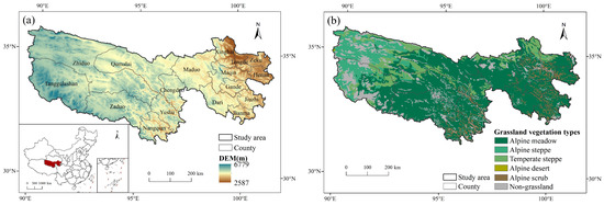
Figure 1.
The Three–River–Source Region: (a) digital elevation model and location; (b) grassland vegetation types.
2.2. Data Collection and Processing
In this study, we primarily utilized Moderate Resolution Imaging Spectroradiometer (MODIS) data, temperature, precipitation, sunshine hours, grassland vegetation types, the number of year–end livestock, population density, and field survey data. Among them, MODIS data, along with temperature, precipitation, sunshine hours, and grassland vegetation types, were used to calculate regional NPP, grassland yield, and theoretical livestock carrying capacity. Data on livestock year–end stock and population density were employed for calculating and spatializing actual livestock carrying capacity, while field survey data were used to verify the accuracy of grassland yield.
- (1)
- MODIS Data. Normalized Difference Vegetation Index (NDVI) and Land Surface Water Index (LSWI) data were obtained from the MODIS vegetation index product (MOD13Q1) for 2010–2022 (16–day composite, spatial resolution of 250 m) downloaded from Google Earth Engine (https://earthengine.google.com, accessed on 5 December 2023). This tertiary product of MODIS, developed by the National Aeronautics and Space Administration (NASA) and the MODIS team of America, which has undergone preprocessing such as radiometric calibration and image correction, was processed through scale reduction, band extraction, stitching, mosaicking, and reprojection. Using the MOD13Q1 products, we generated monthly NDVI data based on Maximum Value Composites (MVCs) to minimize the influence of noise (e.g., clouds, water bodies, snow and ice, atmosphere). Additionally, annual LSWI data were synthesized based on median values.
- (2)
- Temperature and precipitation data. These data were sourced from National Tibetan Plateau/Third Pole Environment Data Center (https://data.tpdc.ac.cn, accessed on 15 December 2023). Temperature data were obtained from the month–by–month mean temperature dataset at a 1 km resolution in China [27], averaged over the 12 months of the year, and resampled to 250 m resolution using the nearest neighbor method (NNM). Precipitation data were derived from the Chinese 1 km resolution month–by–month precipitation dataset [28], summed over the 12 months of the year, and resampled to 250 m resolution. Both datasets were generated from the global 0.5° climate dataset published by CRU and the global high–resolution climate dataset published by WorldClim, using the Delta spatial downscaling scheme for the Chinese region. These datasets were validated using data from 496 independent meteorological observation sites and were credible [29].
- (3)
- Sunshine hours data. These data were sourced from the Geographic Data Sharing Infrastructure, global resources data cloud (www.gis5g.com, accessed on 18 December 2023). Based on annual sunshine hours data from 824 meteorological stations across China, the dataset was strictly quality–controlled and screened. Spatial interpolation was performed using the spline method of the ANUSPLIN software (version 4.3), achieving a spatial resolution of 1 km, which was then resampled to 250 m using the NNM. Digital elevation model (DEM) data were obtained from the Resource and Environmental Science Data Platform (https://www.resdc.cn, accessed on 25 October 2023), calculated based on the SRTM 90 m data measured by NASA and NIMA, and resampled to generate 250 m spatial resolution data using the latest SRTM V4.1. Due to the coarse spatial resolution of existing solar radiation data, we downloaded ERA5–Land 10 km resolution solar radiation data from Google Earth Engine and used the random forest downscaling method to generate solar radiation data with a spatial resolution of 250 m, based on the resampled sunshine hours and DEM data [30].
- (4)
- Grassland vegetation types data. These data were sourced from the national 1:1,000,000 vegetation type map provided by the National Cryosphere Desert Data Center (http://www.ncdc.ac.cn, accessed on 11 December 2023). It was resampled to a resolution of 250 m and reclassified according to the scheme proposed by Ge et al. [31], based on the vegetation map of Qinghai Province. The spatial distributions of grassland types were then extracted and further analyzed.
- (5)
- Actual livestock carrying capacity data. The data were derived and spatialized from the number of livestock at the end of the year, combined with population density, DEM, and NPP. The year–end livestock numbers for each county from 2010 to 2019 were obtained from the National Tibetan Plateau/Third Pole Environment Data Center (https://data.tpdc.ac.cn, accessed on 24 April 2024) [32], while those from 2020 to 2022 were sourced from TRSR state and county statistical yearbooks and bulletins. Population density data for spatialization were retrieved from the LandScan global population density spatial distribution dataset (https://landscan.ornl.gov, accessed on 22 June 2024), originally at a 1 km resolution and resampled to 250 m.
- (6)
- Field survey data. In order to verify the calculation results of the CASA model, the field investigated grassland yield, sourced from the National Forestry and Grassland Administration of China (http://www.forestry.gov.cn/, accessed on 24 November 2023) [33], were utilized in this study. The field survey was conducted during the peak growth period of pasture grasses (July–August). Two to three 1 m × 1 m quadrats were set up within each sampling plot. In each quadrat, all above–ground components of the grassland vegetation, along with the litter, were collected using scissors and subsequently placed in labeled envelopes. The longitude, latitude, altitude, fresh weight of grassland yield, and major plant species of each quadrat were meticulously recorded. The fresh grass was then dried in an oven at 65 °C for 2 d and weighed to obtain the dry weight data of alpine grassland yield.
2.3. Calculation of Forage–Livestock Balance
2.3.1. Calculation of NPP by Improved CASA Model
The CASA model is a widely used model for calculating NPP of vegetation, which is a light energy utilization model based on remote sensing parameters, meteorological conditions, vegetation types, and soil types. The model requires fewer parameters and allows for extensive and long–term NPP estimates with high accuracy based on remote sensing data [24]. Originally developed for the vegetation of North America, the CASA model has been improved to meet various needs [34,35,36]. Notably, Zhu et al. (2007) [37] incorporated vegetation types into the model, determining the maximum NDVI and maximum light energy utilization for different vegetation types. This improvement made the model more suitable for estimating the NPP of Chinese vegetation. Therefore, in this study, the NPP in the TRSR was estimated using Zhu’s (2007) CASA model, with the following equations:
where APAR(x,t) represents the photosynthetically active radiation absorbed by pixel x in month t (); denotes the actual light energy utilization rate of pixel x in month t (gC·MJ−1); SOL(x,t) signifies the total solar radiation of pixel x in month t (); the constant 0.5 represents the ratio of solar photosynthetically active radiation to total solar radiation; FPAR(x,t) represents the fraction of photosynthetically active radiation absorbed by vegetation, which has a good linear relationship with NDVI and SR; and represent the stress effects of low temperature and high temperature on light energy utilization, respectively, while is the water stress coefficient; denotes the maximum light energy utilization rate () under ideal conditions, which varies for different vegetation types based on previous research [38,39,40]; indicates the optimum temperature for plant growth, defined by Zhu et al. (2007) [37] as the average temperature (°C) of the month when NDVI reaches its annual peak in a given region; and EET(x,t) and PET(x,t) denote the regional actual evapotranspiration (mm) and potential evapotranspiration (mm), respectively.
However, the calculation of the water stress coefficient, a key parameter in the model, involves many soil parameters and is primarily based on empirical formulas, which will omit differences in surface vegetation and lead to poor simulation results in arid and semi–arid ecosystems. Traditionally, the water stress coefficient in the CASA model is calculated using spatially interpolated precipitation and temperature data, which can be limited by spatial precipitation constraints. LSWI is a representative parameter of leaf and canopy water content as well as soil moisture, which is calculated from near–infrared and short–wave infrared bands [41]. Higher LSWI values indicate greater canopy water content, while lower values indicate more severe canopy water stress. Previous studies have successfully used LSWI to improve the CASA model, accurately estimating the water stress coefficients. This method has been validated across various ecosystems, including evergreen coniferous forests, temperate deciduous forests, tropical evergreen forests, and (semi–)arid grassland ecosystems.
Xiao et al. (2004) [42] were the first to apply LSWI to calculate water stress in the VPM model. Further, Bao et al. (2016) [43] proposed a modified algorithm to control the range of water stress coefficients from 0.5 to 1. However, the water stress values obtained per pixel by this algorithm did not align with the range of derived from Equation (6), which is from 0.5 (under extreme drought conditions) to 1 (under very wet conditions). This range was effectively reversed compared to the original range, where 0.5 indicated very wet conditions and 1 indicated very dry conditions. Therefore, this study proposes an improved CASA model algorithm to calculate the water stress coefficients based on LSWI, ensuring that the result values range from 0.5 in extreme drought conditions to 1 in very wet conditions, consistently with the original model’s implications. Additionally, most existing studies use the NIR and SWIR1 bands to calculate the surface water index LSWI. However, the spatial resolution of the SWIR1 band in MODIS is only 500 m, and downscaling to 250 m can cause accuracy loss and introduce small errors between different data products. To address this, we use the MOD13Q1 data with 250 m resolution for both the NIR and SWIR2 (i.e., MIR) bands to calculate LSWI. The improved equations for this study are as follows:
where LSWI is the land surface water index, with and representing the near–infrared and mid–infrared bands of the MOD13Q1 data, respectively. The improved water stress coefficient in this study, , is calculated with and denoting the maximum and minimum LSWI values during the growth period of a single image. The theoretical basis for the improvement in Equation (8) lies in the calculation of the standardized index.
2.3.2. Calculation of Grassland Yield
The grassland NPP is the material basis for sustaining grassland ecosystems and a crucial indicator for evaluating their sustainable development. Its accumulation primarily manifests as the grassland yield, which is a vital supply function of grasslands and underpins the development of grassland livestock husbandry. This yield is essential for the rational utilization of grassland resources and for achieving a balance in livestock carrying capacity [44]. Moreover, it serves as a critical parameter for calculating the theoretical livestock carrying capacity. Since the NPP encompasses both aboveground and belowground components, this study estimates the grassland yield based on the NPP calculated using the improved CASA model, applying the belowground–to–aboveground ratio for various grassland types as proposed by Gill et al. [45]:
where represents the unit area grassland yield; t is the biomass conversion coefficient to productivity, set at 0.45 [46]; BNPP is the net primary productivity of the belowground part of the grassland; and ANPP is the net primary productivity of the aboveground part. The ratios of belowground to aboveground productivity for different grassland vegetation types are referenced from studies by Piao et al. [47] and Fan et al. [21].
Given the challenges in collecting NPP data, measured grassland yield is generally converted to NPP to verify accuracy. In this study, as we used the grassland yield to carry out the calculation of livestock carrying capacity, we then directly used the measured grassland yield dry weight and NPP–converted grassland yield to verify the accuracy of the results.
2.3.3. Spatialization of Actual Livestock Carrying Capacity and Evaluation of Forage–Livestock Balance
After calculating the grassland yield based on NPP, the theoretical livestock carrying capacity was further calculated, while the actual livestock carrying capacity was calculated based on the year–end livestock number in each county:
In Equation (10), represents the grassland actual livestock carrying capacity, denotes the supplemental feeding rate, which accounts for 34.24% of the total forage including artificial grassland, silage and straw as indicated in the literature [44]; refers to the livestock number at the end of the year, converted into standard sheep units, with a large livestock equating to four sheep units; signifies the livestock turnout rate, set at 15% in Qinghai Province [46]; and represents the grazing period, calculated as 365 days. The grassland area () is obtained from the national 1:1,000,000 vegetation type map.
In Equation (11), stands for the theoretical livestock carrying capacity, while is the grass availability; the utilization rate of pasture () is set at 70%, and the ratio of edible pasture () is set at 80% [15,48]; represents the amount of food per goat unit per day, calculated as 4 kg of fresh grass per day; and is the ratio of dry weight to fresh weight. The values for and vary for different grassland vegetation types and are determined according to the agricultural industry standard of China [49].
Since the year–end livestock numbers are only accurate to the county level, the calculated actual livestock carrying capacity results in tabular data based on administrative divisions. This lack of spatial accuracy complicates the analysis of the distribution pattern of the actual livestock carrying capacity on a finer spatial scale. To address this, it is essential to spatialize the actual livestock carrying capacity in the TRSR. In this study, we followed the method for spatializing livestock carrying capacity as outlined by the National Tibetan Plateau/Third Pole Environment Data Center [50]. Based on the actual livestock carrying capacity obtained from Equation (11), we performed a multiple linear regression using the population density, NPP, and DEM to establish a spatial model of the actual livestock carrying capacity. However, the model’s calculation results did not completely align with the actual field observations. Therefore, following the studies by Liao et al. [51] and Liu et al. [52], we corrected the model’s calculation results. The method of correction was to interpolate the residuals by Kriging and add them with the results of the model, which was based on the fact that the predicted value of the regression equation and the residuals added together equaled to the actual observed value of the samples.
In this study, the grassland livestock carrying pressure index was employed to evaluate the forage–livestock balance condition in the TRSR:
In Formula (12), represents the livestock carrying pressure index of the grassland, denotes the actual livestock carrying capacity, and is the theoretical livestock carrying capacity. When , it indicates that the actual and theoretical livestock carrying capacity are equivalent, suggesting that the grassland carrying capacity is optimal and suitable for the livestock. When , the actual livestock carrying capacity exceeds the theoretical capacity, indicating an overload state for the grassland. Conversely, when , it suggests that the actual livestock carrying capacity is lower than the theoretical capacity, implying that the grassland still has potential for additional livestock carrying [21]. Based on previous studies [46,53], the livestock carrying pressure index is categorized as follows: insufficient (), balanced (), slightly overloaded (), moderately overloaded (), and severely overloaded ().
2.3.4. Trend Analysis of Time Series
A trend analysis of time series data are often conducted using the linear regression method [54] and Theil–Sen Median method [55,56]. In this study, Theil–Sen Median trend analysis and the Mann–Kendall test were employed to analyze NPP, grassland yield, theoretical livestock carrying capacity, actual livestock carrying capacity and livestock carrying pressure in the TRSR. The Theil–Sen Median method is a robust nonparametric statistical approach, which, compared to the linear regression method, is more resilient to data errors and does not depend on the data distribution. This robustness makes it well–suited for long–term vegetation time series analysis. The method calculates the median of the slopes of lines formed by pairs of data points [57], calculated as follows [58,59]:
where i is the year when the phase starts, j is the year when the phase ends, and represent the NPP, grassland yield, theoretical livestock carrying capacity, actual livestock carrying capacity and livestock carrying pressure for the corresponding years (2010 ≤ I < j ≤ 2022). β > 0 indicates that the time series is increasing and vice versa.
The Mann–Kendall test, a nonparametric statistical test, was used to determine the significance of these trends with the following formula:
where S denotes the Mann–Kendall statistic, positive (or negative) values of Z show an upward (or downward) trend, n represents the length of the time series, and in this study, n = 13, 2010 ≤ i < j ≤ 2022. At a given significant level α, the original hypothesis is rejected and the time series is considered to have a significant change in the α level when [60]. For this paper, we take , and then the critical value = ±1.96; when , it means that the trend passes the significance test with 95% confidence level.
Since there is basically no region with β = 0, this paper refers to the studies of Yuan et al. [60] and Wang et al. [57], and according to the results of Theil–Sen estimation for each time series, we take the threshold . The region of between − and is regarded as basically stable, indicates that the time series has an increasing tendency, signifies a decreasing tendency, and the values of are different for different time series. The criteria for evaluating the change in the trend of the time series were constructed based on the Theil–Sen Median estimation and the Mann–Kendall test, as shown in Table 1.

Table 1.
Classification criteria for the change trend.
3. Results
3.1. Spatiotemporal Patterns of NPP, Grassland Yield, and Theoretical Livestock Carrying Capacity from 2010 to 2022
In this study, the grassland NPP in the TRSR from 2010 to 2022 was calculated using the improved CASA model. The trend of regional grassland NPP over this 13-year period was analyzed according to the classification criteria in Table 1, with the results presented in Figure 2a,b. The grassland NPP in the TRSR during this period displayed a spatial pattern of gradual decrease from southeast to northwest. The average annual NPP was 145.44 gC/m2, with the highest value recorded in 2018 (162.65 gC/m2) and the lowest in 2022 (127.96 gC/m2). Overall, the annual average NPP showed an increasing trend. However, in April 2022, some areas in the TRSR experienced mild to severe drought, with precipitation decreasing by more than 80% compared to the same period in previous years, this resulted in a decrease in NDVI and a significant drop in the NPP. During the 13-year period, grassland NPP in the TRSR increased at a rate of approximately 0.34 gC/m2/year. Of the total area, 46.8% showed an increase in grassland NPP, 36.73% exhibited degradation, and 16.47% remained essentially unchanged. The western part of the TRSR showed little change, while degraded areas were primarily located at the joint areas of Qumalai and Zhiduo Counties, as well as Henan, Gande, Jiuzhi, and Banma Counties. Conversely, the NPP increased in other areas, indicating that the eco–construction projects in the Three–River–Source Nature Reserve have been effective.
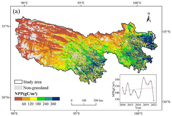
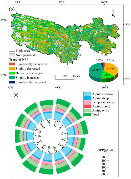
Figure 2.
The spatiotemporal patterns of grassland NPP in the TRSR from 2010 to 2022: (a) mean annual NPP: the inset chart shows the interannual dynamics of NPP from 2010 to 2022, where the red dashed line shows the overall trend of NPP; (b) change trend of NPP: the inset chart shows the area proportion of each; (c) radial accumulation bar chart of NPP in different grassland vegetation types from 2010 to 2022.
Among different grassland vegetation types, alpine meadow had the highest NPP, while alpine desert had the lowest, in counterclockwise order from 2010 to 2022 (Figure 2c). Significant changes in each grassland type were minimal, with the proportion of grassland in a growing state being higher than the proportion experiencing degradation. However, in most areas of the alpine desert, the NPP remained unchanged (Table 2).

Table 2.
Mean of NPP in different grassland vegetation types in the TRSR and the percentage of change trend from 2010 to 2022.
According to the method proposed by Gill et al., the NPP was converted to grassland yield using Equation (9) (Figure 3a,b). Subsequently, the theoretical livestock carrying capacity was calculated according to Equation (11) (Figure 3c,d). Similarly to the NPP, both the grassland yield and theoretical livestock carrying capacity in the TRSR exhibited a spatial pattern of gradual decrease from southeast to northwest, while showing a general upward trend from 2010 to 2022. The average grassland yield was 922.7 kg/hm2 and the average theoretical livestock carrying capacity was 0.55 SU/hm2, with the highest and lowest values occurring in 2018 and 2022, respectively, mirroring the trend observed for the NPP.
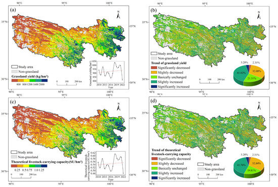
Figure 3.
The spatiotemporal patterns of grassland yield and theoretical livestock carrying capacity in the TRSR from 2010 to 2022: (a) mean annual grassland yield: the inset chart shows the interannual dynamics of grassland yield from 2010 to 2022, where the red dashed line shows the overall trend of grassland yield; (b) change trend of grassland yield: the inset chart shows the area proportion of each; (c) mean annual theoretical livestock carrying capacity: the inset chart shows the interannual dynamics of theoretical livestock carrying capacity from 2010 to 2022, where the red dashed line shows the overall trend of theoretical livestock carrying capacity; (d) change trend of theoretical livestock carrying capacity: the inset chart shows the area proportion of each.
In order to validate the effectiveness of the CASA model improvements proposed in this paper, we used the MOD17A3HGF product with 500 m spatial resolution as the NPP validation dataset. We fitted the NPP calculated in this study to the NPP bands of MOD17A3 (Figure 4a). Additionally, we validated the NPP conversion to grassland yield using field–measured grassland yield data (Figure 4b), taking 2012 as an example. The results show that the improved CASA model in this paper simulated the NPP with high accuracy (R2 = 0.84, p < 0.001). Furthermore, there was a high correlation (R2 = 0.73, p < 0.001) between measured and simulated grassland yield. The validation results from both datasets indicate that the findings of this study are highly reliable.
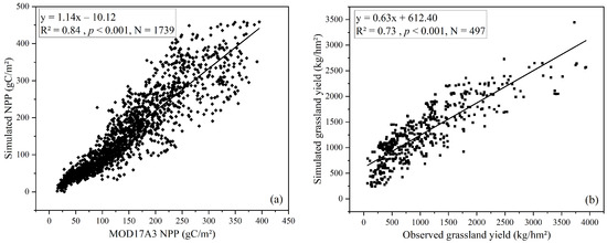
Figure 4.
Validations of simulated NPP and grassland yield by improved CASA model: (a) the correlation of simulated NPP by improved CASA model and MOD17A3 NPP, where the solid black line represents the fitting curve of simulated NPP and MOD17A3 NPP; (b) the correlation of simulated grassland yield by improved CASA model and observed grassland yield, where the solid black line represents the fitting curve of simulated grassland yield and observed grassland yield.
3.2. Spatiotemporal Patterns of Actual Livestock Carrying Capacity from 2010 to 2022
The actual livestock carrying capacity of counties in the TRSR from 2010 to 2022 was calculated based on Equation (10), using the year–end livestock numbers from the statistical yearbook (Table 3). For Tanggulashan Town, where data were missing, we substituted the data for Golmud City, its administrative location. The results indicated that the actual livestock carrying capacity was higher in the eastern and southern regions of the TRSR. Notably, Tongde and Henan Counties in the northeast exhibited significantly higher actual livestock carrying capacity compared to other regions.

Table 3.
Actual livestock carrying capacity of counties in the TRSR from 2010 to 2022.
Since the statistical data of year–end livestock counts are only accurate to the county scale, this study spatialized the actual livestock carrying capacity in Table 3 based on the population density, DEM, and NPP calculated by the improved CASA model to analyze changes in spatial patterns. The mean absolute error (MAE) of the spatialization was 0.26 SU/hm2, and the mean square error (MSE) was 0.11 SU/hm2.
The spatialized mean and trend of actual livestock carrying capacity from 2010 to 2022 are shown in Figure 5. The TRSR exhibits distinct spatial distribution characteristics, with a higher livestock carrying capacity in the east and lower in the west. The northeast region, in particular, shows a significantly higher livestock carrying capacity (Figure 5a). This disparity is mainly due to the northeast’s denser population of people engaged in animal husbandry, more abundant pastures, and better grassland growth, allowing it to support more livestock. During the 13–year period, the actual livestock carrying capacity decreased at an average rate of 0.0015 SU/hm2/year. The annual average livestock carrying capacity was 0.46 SU/hm2, peaking in 2020 at 0.51 SU/hm2, before sharply declining to a minimum of 0.42 SU/hm2 in 2021. This fluctuation was influenced by the global epidemic in 2020, which caused a significant decrease in livestock turnout rates in some areas, resulting in higher year–end livestock values and increased actual livestock carrying capacity. In 2021, coordinated efforts in the TRSR to promote economic recovery and development led to an increase in livestock turnout rates and agricultural and animal husbandry output, reducing year–end livestock numbers and decreasing actual livestock carrying capacity. From 2010 to 2022, the actual livestock carrying capacity significantly increased in Tanggulashan Town, Zhiduo, Qumalai, and Maduo Counties, while Zaduo County and the eastern part of the TRSR saw significant decreases (Figure 5b). As shown in Table 3, Tanggulashan Town and Maduo County experienced a notable increase in 2020 due to the small base of livestock carrying capacity, but it remained stable in other years. Qumalai County saw a significant increase in livestock carrying capacity from 2014 to 2016, followed by a gradual decrease. Zhiduo County experienced a gradual increase in livestock carrying capacity starting in 2015, which later stabilized. Overall, the eastern region saw a significant effect from livestock reduction, with 36.01% of the area experiencing a decrease in actual livestock carrying capacity, including 12.07% with a significant decrease.
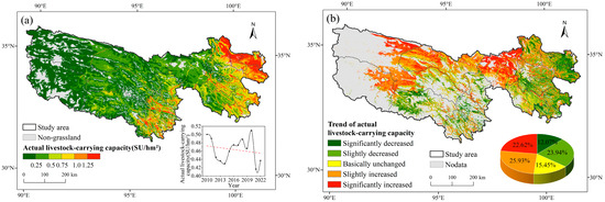
Figure 5.
The spatiotemporal patterns of actual livestock carrying capacity in the TRSR from 2010 to 2022: (a) mean annual actual livestock carrying capacity: the inset chart shows the interannual dynamics of actual livestock carrying capacity from 2010 to 2022, where the red dashed line shows the overall trend of actual livestock carrying capacity; (b) change trend of actual livestock carrying capacity: the inset chart shows the area proportion of each.
3.3. Evaluation of Forage–Livestock Balance in the TRSR from 2010 to 2022
The livestock carrying pressure index was divided into five categories, and the spatial distribution and trend of changes were obtained, as shown in Figure 6. Over the past 13 years, the TRSR as a whole has maintained a forage–livestock balance, with an average livestock carrying pressure index of 0.96. However, serious overloading was observed in the western part of Qumalai County and the northern part of Tongde County, while Zhiduo, Maduo, and Zeku Counties experienced slight overloading (Figure 6a). An analysis revealed that the causes of overloading varied across different areas in the TRSR. In Qumalai, Zhiduo, and Maduo Counties, the theoretical livestock carrying capacity was low due to poor grassland growth, but even though the actual livestock carrying capacity was low, there were overgrazing problems. Tongde and Zeku Counties had a high actual livestock carrying capacity and were densely populated, so there was severe overloading. From 2010 to 2022, the livestock carrying pressure increased at a rate of about 0.03 per year, with the lowest pressure observed in 2019 (0.78) and a steep increase in 2020, reaching a peak in 2022 (1.4). The increase in 2020 was attributed to the global pandemic, which led to an increase in the actual livestock carrying capacity and, consequently, a higher livestock carrying pressure index. In 2022, extreme drought significantly decreased the NPP and theoretical livestock carrying capacity, further increasing the livestock carrying pressure index. The trend of the livestock carrying pressure index mirrored that of the actual livestock carrying capacity, with significant increases in Tanggulashan Town, Zhiduo, Qumalai, and Maduo Counties, and significant decreases in Zaduo County and the eastern region. The livestock–carrying pressure decreased in 34.76% of the areas and remained basically unchanged in 19.43% of the areas (Figure 6b). Overall, the ecological protection and construction projects in the TRSR have had positive impacts. In the future, it is essential to continue strengthening the rotational grazing system and forage–livestock balance management. Implementing a comprehensive grazing ban policy for seriously degraded grassland and continuing the policy of returning pasture to grassland and reducing livestock in areas with higher livestock carrying pressure are crucial, so as to promote ecosystem restoration and achieve ecological balance and harmonious coexistence between humans and nature.
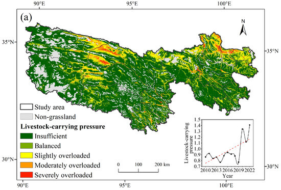
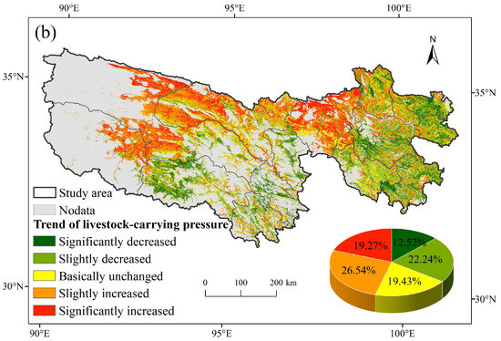
Figure 6.
The spatiotemporal patterns of the livestock carrying pressure in the TRSR from 2010 to 2022: (a) mean annual livestock carrying pressure: the inset chart shows the interannual dynamics of livestock carrying pressure from 2010 to 2022, where the red dashed line shows the overall trend of livestock carrying pressure; (b) change trend of livestock carrying pressure: the inset chart shows the area proportion of each.
4. Discussion
4.1. Improvement of the CASA Model
Based on the improvements made by Bao et al. [43], we further improved the CASA model to obtain a more suitable NPP calculation model for grassland ecosystems in the plateau region. We specifically improved the water stress coefficient and compared the results with the CASA model from Zhu (2007) [37] (Figure 7). The MOD17A3HGF NPP product (version 6.1) from NASA, based on the Terra satellite platform and derived from the light energy utilization model and Biome-BGC model, has been widely used and tested in carbon cycle and biomass estimation studies, effectively reflecting global ecosystem NPP changes [61]. This product corrects issues related to response and scanning angle methods affecting the reflectivity bands of Aqua and Terra MODIS and addresses optical crosstalk in the infrared band of Terra MODIS, ensuring high recognition accuracy [62]. Consequently, we selected the MOD17A3 product as a verification reference to assess the improvements in our CASA model.
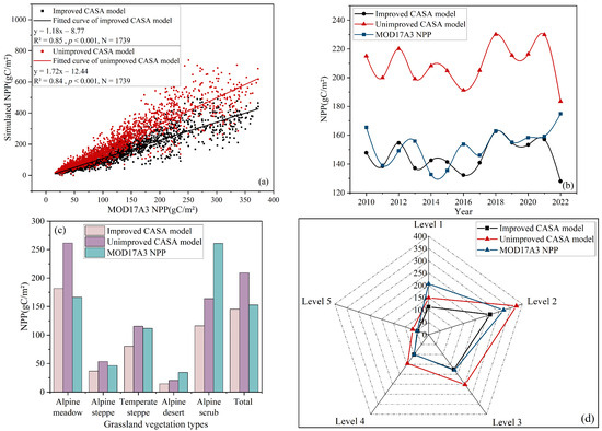
Figure 7.
Simulated NPP by improved CASA model and unimproved CASA model compared to MOD17A3 NPP product: (a) scatter plot with MOD17A3 NPP; (b) change curve of NPP from 2010 to 2022; (c) histogram of NPP in different grassland vegetation types; (d) radar map of NPP with different elevation grades.
Figure 7a illustrates the fitted scatter plots of NPP compared with the MOD17A3 product before and after model improvements, using 1739 random points for verification. The proposed model’s random point distribution aligns with that of the Zhu (2007) model. The regression fitting R2 of the improved CASA model with the added land surface water index is slightly better than that of the Zhu (2007) model, with the fitting curve closer to the MOD17A3 product reference values, with the overall result of the Zhu (2007) model being higher than the reference values. Figure 7b compares the NPP change curves of MOD17A3 product from 2010 to 2022 before and after the model improvement. The overall trend and value of the improved model’s NPP curve closely match those of MOD17A3. The average NPP calculated by our improved CASA model over 13 years is 145.44 gC/m2, close to the MOD17A3 average (149.55 gC/m2), with a significant difference only in 2022. The trend of the CASA model remains consistent before and after improvement, suggesting that the differences in individual years between our model and MOD17A3 are due to different calculation models, data sources, and parameters. Figure 7c compares the CASA model and MOD17A3 product across different grassland vegetation types before and after improvement. It can be observed from the map of grassland vegetation types that alpine meadow and alpine steppe constitute about 80% of the total grassland area in the TRSR, with alpine meadow alone accounting for about 67.4%. So, the results of the improved model align closely with MOD17A3 for alpine meadow, alpine steppe, and the overall grassland ecosystem, with differences observed only in alpine scrub, which accounts for only 6.6% of the total grassland area in the TRSR. This has a minimal impact on the overall results, indicating that the improved model is suitable for grassland ecosystem in the TRSR. The unimproved model shows greater similarity to MOD17A3 for temperate steppe and alpine desert, while both models significantly differ from MOD17A3 for alpine scrub, necessitating further model parameter improvements in the future. To evaluate NPP variations at different elevations and the model’s accuracy, we divided the research area into six elevation levels: Level 1 (2587–3200 m), Level 2 (3200–3900 m), Level 3 (3900–4600 m), Level 4 (4600–5300 m), Level 5 (5300–6000 m), and Level 6 (6000–6779 m). Since there is no grassland in Level 6, the grassland NPP in the first five grades is analyzed (Figure 7d). As elevation increases, NPP initially rises and then falls, peaking at Level 2 and reaching its lowest value at Level 5. Additionally, our improved CASA model closely aligns with MOD17A3 at Levels 3, 4, and 5, but showing significant discrepancies at Level 1. In contrast, the unimproved model closely matches MOD17A3 at Level 5 but differs significantly at other elevation levels. Thus, the improved CASA model demonstrates a strong performance for the grassland ecosystem in the plateau area.
4.2. Changes in Livestock Carrying Pressure by Counties
The livestock carrying pressure in each county of the TRSR from 2010 to 2022 is shown in Figure 8a, in which areas with a lower livestock carrying pressure are depicted in deeper blue, while areas with a higher pressure are shown in deeper red. As illustrated, Zeku, Xinghai, and Tongde Counties face significant overloading issues. Although there was some relief in 2018 and 2019, overloading began to escalate again from 2020 onwards in Zeku, Xinghai, Tongde, Zhido, and Qumalai Counties. Apart from these five counties and Maduo County in 2020, the other areas maintained a forage–livestock balance over the 13 years (). Since the implementation of ecological engineering and grazing ban policies in the TRSR, the central and western counties have consistently maintained a forage–livestock balance, while the eastern region suffers severe overloading. This discrepancy is linked to ecological migration in the central region and livestock fattening projects in the eastern region [44]. In the northeastern counties of Zeku, Xinghai, and Tongde, with less natural pasture area, a relatively dense population and increasing demand for livestock due to population growth have resulted in more livestock being raised [53]. These areas were in a perpetual state of overloading. In 2020, the global pandemic led to a significant reduction in the livestock outbreeding rate in some areas, causing an increase in year–end livestock numbers and actual livestock carrying capacity. Consequently, the livestock carrying pressure index rose sharply compared to 2019. Additionally, decreased temperature and solar radiation in the western and northeastern parts of Zhido County and the western part of Qumalai County led to a reduction in NPP and theoretical livestock carrying capacity, further increasing the livestock carrying pressure index in these areas. Despite a decrease in actual livestock carrying capacity in Xinghai, Tongde, and Qumalai Counties in 2022, livestock carrying pressure remained high due to a significant reduction in NPP. Figure 8b presents a column chart where pink columns indicate an increase in livestock carrying pressure, and green columns indicate a decrease. The trend line represents the average livestock carrying pressure index in each county for 13 years. It is evident that more than half of the administrative areas have experienced increased livestock carrying pressure, predominantly in the eastern, densely populated regions of the TRSR. Zhido and Qumalai Counties have also seen a significant rise in livestock carrying pressure due to reduced NPP, with Tongde County having the highest average livestock carrying pressure and Tanggulashan Town the lowest.
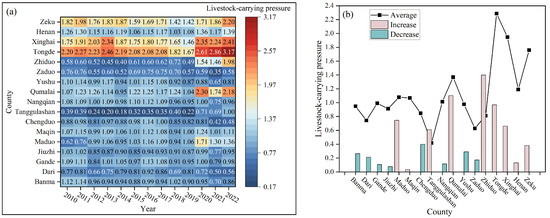
Figure 8.
Livestock carrying pressure in the TRSR from 2010 to 2022: (a) heat map of livestock carrying pressure in each county from 2010 to 2022; (b) changes and average values of livestock carrying pressure in each county for 13 years.
4.3. Analysis of Forage–Livestock Balance in the Three–River–Source Nature Reserve
Since 2005, ecological protection and construction projects have been carried out in the TRSR, encompassing 18 nature reserves divided into a core zone, buffer zone, and experimental zone. Among them, the core zone is strictly protected, with the restoration of forest and grass vegetation achieved through measures such as grazing and cutting bans. The buffer zone is designated as a key protected area, where grassland degradation should be controlled, restricted grazing and rotational grazing practiced based on forage availability. The experimental zone, serving as a general protection area, focuses on the restoration and reconstruction of degraded ecosystems while developing characteristic industries such as eco–tourism and the regional economy. Figure 9 illustrates the superimposition of the distribution of actual livestock carrying capacity, livestock carrying pressure, NDVI, and the Three–River–Source Nature Reserve. It was observed that the actual livestock carrying capacity in the core zone was low (Figure 9a), indicating that the implementation of the ecological project has yielded remarkable outcomes. Consequently, the grazing prohibition policy in the core zone of the protected area should be strictly enforced in the future. However, Figure 9b reveals that the core protected areas in Zhiduo and Qumalai Counties experience relatively severe overload, despite the actual livestock carrying capacity not being high. This issue is primarily attributed to the low theoretical livestock carrying capacity caused by the low NDVI value in this region (Figure 9c), which results in high livestock carrying pressure in the core zone of the protected area. In this area, it is necessary to control livestock based on forage availability, strengthen the policy of returning grazing land to grassland in the nature reserve, promote grassland restoration and reduce livestock carrying pressure based on the actual productivity of the grassland.
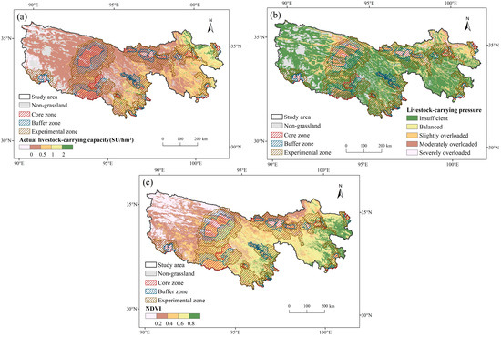
Figure 9.
The spatial distributions of grazing condition and Three–River–Source Nature Reserve (https://sthjt.qinghai.gov.cn, accessed on 14 July 2024) from 2010 to 2022: (a) mean annual actual livestock carrying capacity; (b) mean annual livestock carrying pressure; (c) mean annual NDVI.
4.4. Limitations and Uncertainties
Regarding the improvement of the CASA model and the spatialization of actual livestock carrying capacity at the county scale, this study has some limitations: (1) The improved CASA model in this paper is applicable to grassland ecosystem in the TRSR; however, its accuracy needs to be improved in low–altitude areas and smaller temperate steppe and alpine scrub within the region. (2) In this paper, the situation of regional NPP is referenced when spatializing the actual livestock carrying capacity, meaning the accuracy of the CASA model significantly impacts the actual livestock carrying capacity. With only 17 administrative units in the research area, fewer variables were included in the model construction for actual livestock carrying capacity. Therefore, the spatial results needed optimization, and we revised the results by including residuals. In future studies, the research scope will be further expanded, and the regression model will be optimized to improve the precision of livestock carrying capacity spatialization. (3) This study only considers the forage supply and the state of forage–livestock balance during the year, without covering the stocking conditions of forage pastures in the “cold season” and “warm season.” Therefore, it is difficult to address the widespread seasonal overloading problem in grazing areas [63]. Future research could be conducted considering grazing during the cold and warm seasons.
5. Conclusions
In this study, an improved CASA model was proposed for the grassland ecosystem in the TRSR, and the actual livestock carrying capacity was spatialized to analyze the forage–livestock balance. The enhanced CASA model presented in this paper is adeptly suited for grassland ecosystems within alpine regions, which are not readily constrained by spatial precipitation. It demonstrates a commendable fitting accuracy in expansive areas of alpine meadow and alpine steppe. Nevertheless, the model exhibits certain deficiencies; specifically, its accuracy in lower elevation zones and smaller expanses of temperate steppe and alpine scrub requires enhancement. Additionally, there is a pressing need for further refinement of the model parameters, enabling its broader applicability across diverse grassland vegetation types in the future.
The results revealed the following: (1) From 2010 to 2022, 46.8% of the total grassland area in the TRSR was in a state of increasing NPP, whereas 36.73% was in a state of decrease. The degraded areas were primarily distributed at the joint areas of Qumalai and Zhiduo Counties, as well as in Henan, Gande, Jiuzhi, and Banma Counties. Notably, among all grassland vegetation types, alpine meadow had the highest NPP. (2) Moreover, the actual livestock carrying capacity exhibited a spatial pattern of high in the east and low in the west. Specifically, 48.55% of the TRSR area showed an increase in actual livestock carrying capacity, while 36.01% showed a decrease. The areas with an increased actual livestock carrying capacity were predominantly distributed in Tanggulashan Town, Zhiduo, Qumalai, and Maduo Counties. (3) Overall, the study area maintained a forage–livestock balance. However, there were serious overloads in western Qumalai County and northern Tongde County, with slight overloads in Zhiduo, Maduo, and Zeku Counties. Livestock carrying pressure increased in 45.81% of the regions, whereas it decreased in 34.76%. Notably, Tanggulashan Town, Zhiduo, Qumalai, and Maduo Counties experienced significant increases, while Zaduo County and the eastern regions experienced significant decreases. These findings from 2010 to 2022 stress the need for the TRSR to further strengthen the management of the forage–livestock balance, particularly in Qumalai and Tongde Counties, where livestock numbers need to be reduced. The approach of improving the CASA model in this paper can be applied to forage–livestock balance research in other regions. Consequently, these research results hold positive significance for maintaining the regional forage–livestock balance and achieving the sustainable management of alpine grassland.
Author Contributions
Conceptualization, C.H., Y.T., K.Y. and H.H.; methodology, C.H., Y.T., K.Y. and H.H.; validation, C.H. and K.Y.; formal analysis, C.H., K.Y. and H.H.; investigation, C.H. and K.Y.; writing—original draft preparation, C.H.; writing—review and editing, K.Y. and L.L.; visualization, C.H. and L.L.; supervision, Y.T. and Q.C.; funding acquisition, L.L. All authors have read and agreed to the published version of the manuscript.
Funding
This research was funded by the National Natural Science Foundation of China (82274041, 72374017) and the Strategic Priority Research Program of Chinese Academy of Sciences (XDA26010101).
Data Availability Statement
The original contributions presented in the study are included in the article, further inquiries can be directed to the corresponding author.
Acknowledgments
We acknowledge the support of all co-authors for their constructive and helpful comments and organization of this study.
Conflicts of Interest
The authors declare no conflicts of interest.
References
- Parton, W.J.; Schimel, D.S.; Cole, C.V.; Ojima, D.S. Analysis of Factors Controlling Soil Organic Matter Levels in Great Plains Grasslands. Soil Sci. Soc. Am. J. 1987, 51, 1173–1179. [Google Scholar] [CrossRef]
- Scurlock, J.M.O.; Hall, D.O. The Global Carbon Sink: A Grassland Perspective. Glob. Chang. Biol. 1998, 4, 229–233. [Google Scholar] [CrossRef]
- Wang, Y.; Huang, H.; Yang, G.; Chen, W. Ecosystem Service Function Supply–Demand Evaluation of Urban Functional Green Space Based on Multi-Source Data Fusion. Remote Sens. 2022, 15, 118. [Google Scholar] [CrossRef]
- Tongqian, Z.; Zhiyun, O.; Liangqing, J.; Hua, Z. Ecosystem Services and Their Valuation of China Grassland. Acta Ecol. Sin. 2004, 24, 1101–1110. [Google Scholar]
- Sasaki, T.; Okayasu, T.; Ohkuro, T.; Shirato, Y.; Jamsran, U.; Takeuchi, K. Rainfall Variability May Modify the Effects of Long-Term Exclosure on Vegetation in Mandalgobi, Mongolia. J. Arid Environ. 2009, 73, 949–954. [Google Scholar] [CrossRef]
- Zhang, Y.; Zhang, C.; Wang, Z.; Chen, Y.; Gang, C.; An, R.; Li, J. Vegetation Dynamics and Its Driving Forces from Climate Change and Human Activities in the Three-River Source Region, China from 1982 to 2012. Sci. Total Environ. 2016, 563–564, 210–220. [Google Scholar] [CrossRef]
- Feng, X.; Huang, H.; Wang, Y.; Tian, Y.; Li, L. Identification of Ecological Sources Using Ecosystem Service Value and Vegetation Productivity Indicators: A Case Study of the Three-River Headwaters Region, Qinghai–Tibetan Plateau, China. Remote Sens. 2024, 16, 1258. [Google Scholar] [CrossRef]
- Bai, Y.; Guo, C.; Degen, A.A.; Ahmad, A.A.; Wang, W.; Zhang, T.; Li, W.; Ma, L.; Huang, M.; Zeng, H.; et al. Climate Warming Benefits Alpine Vegetation Growth in Three-River Headwater Region, China. Sci. Total Environ. 2020, 742, 140574. [Google Scholar] [CrossRef]
- Wang, X. Conservation value and management model of Three-River-Source National Park. Natl. Park. 2023, 1, 62–66. (In Chinese) [Google Scholar]
- Zhang, J.; Zhang, L.; Liu, W.; Qi, Y.; Wo, X. Livestock-Carrying Capacity and Overgrazing Status of Alpine Grassland in the Three-River Headwaters Region, China. J. Geogr. Sci. 2014, 24, 303–312. [Google Scholar] [CrossRef]
- Feng, J.; Wang, T.; Xie, C. Eco-Environmental Degradation in the Source Region of the Yellow River, Northeast Qinghai-Xizang Plateau. Environ. Monit. Assess. 2006, 122, 125–143. [Google Scholar] [CrossRef]
- Li, M.; He, Y.T.; Fu, G.; Shi, P.L.; Zhang, X.Z.; Sun, J.; Li, R.Q.; Wang, J.B. Livestock-Forage Balance in the Three River Headwater Region Based on the Terrestrial Ecosystem Model. Ecol. Environ. Sci. 2016, 25, 1915–1921. [Google Scholar]
- Wang, C.; Wang, J.; Zhang, F.; Li, Y.; Li, H.; Yang, Y.; Luo, F. Climate Resource Utilization Rate and Livestock-Carrying Capacity of Grasslands in the Three River Headwaters Region over the Past 40 Years. Pratac. Sci. 2022, 39, 672–687. [Google Scholar]
- Qin, L.; Song, X.; Feng, X. Forage-Livestock Dynamic Balance of Pasturing Area Based on Rotational Grazing Theory in Northern Slope of Qilian Mountains. Trans. Chin. Soc. Agric. Eng. 2019, 35, 256–264. [Google Scholar]
- Zhang, L.; Fan, J.; Shao, Q.; Tang, F.; Zhang, H.; Li, Y. Changes in Grassland Yield and Grazing Pressure in the Three Rivers Headwater Region before and after the Implementation of the Eco-Restoration Project. Acta Pratac. Sin. 2014, 23, 116–123. [Google Scholar]
- Yu, C.; Zhang, X.; Zhang, J.; Li, S.; Song, C.; Fang, Y.; Wurst, S.; Wu, J. Grazing Exclusion to Recover Degraded Alpine Pastures Needs Scientific Assessments across the Northern Tibetan Plateau. Sustainability 2016, 8, 1162. [Google Scholar] [CrossRef]
- Zhao, L.; Liu, Z.; Hu, Y.; Zhou, W.; Peng, Y.; Ma, T.; Liu, L.; Li, S.; Wang, L.; Mao, X. Evaluation of Reasonable Stocking Rate Based on the Relative Contribution of Climate Change and Grazing Activities to the Productivity of Alpine Grasslands in Qinghai Province. Remote Sens. 2022, 14, 1455. [Google Scholar] [CrossRef]
- Qian, S.; Mao, L.; Hou, Y.; Fu, Y.; Zhang, H.; Du, J. Livestock Carrying Capacity and Balance Between Carrying Capacity of Grassland with Added Forage and Actual Livestock in the Qinghai-Tibet Plateau. J. Nat. Resour. 2007, 22, 389–397. [Google Scholar]
- Lieth, H. Modeling the Primary Productivity of the World. Prim. Product. Biosph. 1975, 14, 237–263. [Google Scholar]
- Qu, Y.; Zhao, Y.; Ding, G.; Chi, W.; Gao, G. Spatiotemporal Patterns of the Forage-Livestock Balance in the Xilin Gol Steppe, China: Implications for Sustainably Utilizing Grassland-Ecosystem Services. J. Arid Land 2021, 13, 135–151. [Google Scholar] [CrossRef]
- Fan, J.-W.; Shao, Q.-Q.; Liu, J.-Y.; Wang, J.-B.; Harris, W.; Chen, Z.-Q.; Zhong, H.-P.; Xu, X.-L.; Liu, R.-G. Assessment of Effects of Climate Change and Grazing Activity on Grassland Yield in the Three Rivers Headwaters Region of Qinghai–Tibet Plateau, China. Environ. Monit. Assess. 2010, 170, 571–584. [Google Scholar] [CrossRef]
- Liu, H.; Song, X.; Qin, L.; Wen, W.; Liu, X.; Hu, Z.; Liu, Y. Evaluation of Forage-Livestock Balance for Pastoral Areas in Arid Sandy Grasslands Using Improved Key Pasture Approach. Trans. Chin. Soc. Agric. Eng. 2021, 37, 294–300. [Google Scholar]
- Holechek, J.L.; Gomez, H.; Galt, D. Grazing Studies: What We’ve Learned. Rangel. Arch. 1999, 21, 12–16. [Google Scholar]
- Zhang, Y. Spatiotemporal Pattern of Vegetation Productivity and Its Driving Forces in the Three Rivers Source Region. Master’s Thesis, Qinghai Normal University, Xining, China, 2021. [Google Scholar]
- Xu, X.; Liu, J.; Shao, Q.; Fan, J. The Dynamic Changes of Ecosystem Spatial Pattern and Structure in the Three-River Headwaters Region in Qinghai Province during Recent 30 Years. Geogr. Res. 2008, 27, 829–838. [Google Scholar]
- Li, H.; Liu, G.; Fu, B. Estimation of Regional Evapotranspiration in Alpine Area and Its Response to Land Use Change: A Case Study in Three-River Headwaters Region of Qinghai-Tibet Plateau, China. Chin. Geogr. Sci. 2012, 22, 437–449. [Google Scholar] [CrossRef]
- Peng, S. 1-Km Monthly Mean Temperature Dataset for China (1901–2022); National Tibetan Plateau Data Center: Beijing, China, 2020. [Google Scholar]
- Peng, S. 1-Km Monthly Precipitation Dataset for China (1901–2022); National Tibetan Plateau Data Center: Beijing, China, 2020. [Google Scholar]
- Peng, S.; Gang, C.; Cao, Y.; Chen, Y. Assessment of Climate Change Trends over the Loess Plateau in China from 1901 to 2100. Int. J. Climatol. 2018, 38, 2250–2264. [Google Scholar] [CrossRef]
- Zhu, W.; Yuan, C.; Tian, Y.; Wang, Y.; Li, L.; Hu, C. A New High-Resolution Rural Built-Up Land Extraction Method Based on Artificial Surface Index with Short-Wave Infrared Downscaling. Remote Sens. 2024, 16, 1126. [Google Scholar] [CrossRef]
- Ge, J.; Meng, B.; Liang, T.; Feng, Q.; Gao, J.; Yang, S.; Huang, X.; Xie, H. Modeling Alpine Grassland Cover Based on MODIS Data and Support Vector Machine Regression in the Headwater Region of the Huanghe River, China. Remote Sens. Environ. 2018, 218, 162–173. [Google Scholar] [CrossRef]
- Liu, Y. County-Level Data on Livestock Stocks and Herds on the Tibetan Plateau, 2000–2019; National Tibetan Plateau Data Center: Beijing, China, 2023. [Google Scholar]
- Li, H. A Machine Learning Scheme for Estimating Fine-Resolution Grassland Aboveground Biomass over China with Sentinel-1/2 Satellite Images. Remote Sens. Environ. 2024, 311, 114317. [Google Scholar] [CrossRef]
- Potter, C.S.; Randerson, J.T.; Field, C.B.; Matson, P.A.; Vitousek, P.M.; Mooney, H.A.; Klooster, S.A. Terrestrial Ecosystem Production: A Process Model Based on Global Satellite and Surface Data. Glob. Biogeochem. Cycles 1993, 7, 811–841. [Google Scholar] [CrossRef]
- Piao, S.; Fang, J.; He, J. Variations in Vegetation Net Primary Production in the Qinghai-Xizang Plateau, China, from 1982 to 1999. Clim. Change 2006, 74, 253–267. [Google Scholar] [CrossRef]
- Wu, Y.; Tan, H.; Deng, Y.; Wu, J.; Xu, X.; Wang, Y.; Tang, Y.; Higashi, T.; Cui, X. Partitioning Pattern of Carbon Flux in a Kobresia Grassland on the Qinghai-Tibetan Plateau Revealed by Field 13 C Pulse-labeling. Glob. Change Biol. 2010, 16, 2322–2333. [Google Scholar] [CrossRef]
- Zhu, W.-Q.; Pan, Y.-Z.; Zhang, J.-S. Estimation of Net Primary Productivity of Chinese Terrestrial Vegetation Based on Remote Sensing. Chin. J. Plant Ecol. 2007, 31, 413–424. [Google Scholar]
- Zhu, W.; Pan, Y.; He, H.; Yu, D.; Hu, H. Simulation of Maximum Light Use Efficiency for Some Typical Vegetation Types in China. Chin. Sci. Bull. 2006, 51, 457–463. [Google Scholar] [CrossRef]
- Wei, Y.; Wang, L. The Study on Simulating Light Use Efficiency of Vegetation in Qinghai Province. Acta Ecol. Sin. 2010, 30, 5209–5216. [Google Scholar]
- Liu, M. Change of Grassland Aboveground Biomass in the Three-River Headwater Region and Analysis of Its Response to Climate Factors. Master’s Thesis, China University of Geosciences, Beijing, China, 2019. [Google Scholar]
- Li, J.; Han, H.; Kang, F.; Hu, B.; Jing, H. Spatiotemporal Dynamics and Climate Impact of Vegetation NPP in the Northern Shanxi Province Region Based on the Improved CASA Model. J. Beijing For. Univ. 2023, 45, 47–60. [Google Scholar]
- Xiao, X.; Hollinger, D.; Aber, J.; Goltz, M.; Davidson, E.A.; Zhang, Q.; Moore, B. Satellite-Based Modeling of Gross Primary Production in an Evergreen Needleleaf Forest. Remote Sens. Environ. 2004, 89, 519–534. [Google Scholar] [CrossRef]
- Bao, G.; Bao, Y.; Qin, Z.; Xin, X.; Bao, Y.; Bayarsaikan, S.; Zhou, Y.; Chuntai, B. Modeling Net Primary Productivity of Terrestrial Ecosystems in the Semi-Arid Climate of the Mongolian Plateau Using LSWI-Based CASA Ecosystem Model. Int. J. Appl. Earth Obs. Geoinf. 2016, 46, 84–93. [Google Scholar] [CrossRef]
- Li, G.; Sun, W.; Zhang, H.; Gao, C. Balance between Actual Number of Livestock and Livestock Carrying Capacity of Grassland after Added Forage of Straw Based on Remote Sensing in Tibetan Plateau. Trans. Chin. Soc. Agric. Eng. 2014, 30, 200–211. [Google Scholar]
- Gill, R.A.; Kelly, R.H.; Parton, W.J.; Day, K.A.; Jackson, R.B.; Morgan, J.A.; Scurlock, J.M.O.; Tieszen, L.L.; Castle, J.V.; Ojima, D.S.; et al. Using Simple Environmental Variables to Estimate Below-ground Productivity in Grasslands. Glob. Ecol. Biogeogr. 2002, 11, 79–86. [Google Scholar] [CrossRef]
- Huang, L.; Ning, J.; Zhu, P.; Zheng, Y.; Zhai, J. The Conservation Patterns of Grassland Ecosystem in Response to the Forage-Livestock Balance in North China. J. Geogr. Sci. 2021, 31, 518–534. [Google Scholar] [CrossRef]
- Piao, S.; Fang, J.; He, J.; Xiao, Y. Spatial Distribution of Grassland Biomass in China. Acta Phytoecol. Sin. 2004, 28, 491–498. [Google Scholar]
- Qian, Q.; Zhang, X.; Wang, J.; Ye, H.; Li, Y.; Zhang, Z. The Spatio-Temporal Pattern of Grazing Pressure in the Three-River Headwaters in Qinghai Province from 2005to 2017. Acta Agrestia Sin. 2021, 29, 1311–1317. [Google Scholar]
- NYT635-2002; Calculation of Rangeland Carrying Capacity. Ministry of Agriculture of the People’s Republic of China: Beijing, China, 2002. (In Chinese)
- Liu, B. Actual Livestock Carrying Capacity Estimation Product in Qinghai-Tibet Plateau (2000–2019); National Tibetan Plateau Data Center: Beijing, China, 2023. [Google Scholar]
- Liao, S.; Qin, Y. A Spatialization Method for Survey Data of Theoretical Stock-Carrying Capacity of Grassland in China and Its Application. Geogr. Res. 2014, 33, 179–190. [Google Scholar]
- Liu, D.; Wang, P.; Yue, X.; Liu, X. GIS based spatial simulation of reasonable carrying capacity of grasslands in China. Grassl. Turf. 2015, 35, 92–96. (In Chinese) [Google Scholar]
- Wang, X. Analysis on the Temporal and Spatial Changes of Grazing Activities and the Balance between Forage and Livestock in the Qinghai-Tibet Plateau from 2000 to 2018. Master’s Thesis, Chang’an University, Xi’an, China, 2022. (In Chinese). [Google Scholar]
- Fensholt, R.; Rasmussen, K.; Nielsen, T.T.; Mbow, C. Evaluation of Earth Observation Based Long Term Vegetation Trends—Intercomparing NDVI Time Series Trend Analysis Consistency of Sahel from AVHRR GIMMS, Terra MODIS and SPOT VGT Data. Remote Sens. Environ. 2009, 113, 1886–1898. [Google Scholar] [CrossRef]
- CAI, B.; YU, R. Advance and Evaluation in the Long Time Series Vegetation Trends Research Based on Remote Sensing. J. Remote Sens. 2009, 13, 1170–1186. [Google Scholar]
- Lunetta, R.S.; Knight, J.F.; Ediriwickrema, J.; Lyon, J.G.; Worthy, L.D. Land-Cover Change Detection Using Multi-Temporal MODIS NDVI Data. Remote Sens. Environ. 2006, 105, 142–154. [Google Scholar] [CrossRef]
- Wang, J.; Cui, K.; Yang, F.; Li, J.; Zhang, C.; Du, T.; Zhang, H. Evaluation of Spatiotemporal Variation and Impact Factors for Vegetation Net Primary Productivity in a Typical Open-pit Mining Ecosystem in Northwestern China. Land Degrad. Dev. 2024, 35, 3756–3770. [Google Scholar] [CrossRef]
- Sen, P.K. Estimates of the Regression Coefficient Based on Kendall’s Tau. J. Am. Stat. Assoc. 1968, 63, 1379–1389. [Google Scholar] [CrossRef]
- Theil, H. A Rank-Invariant Method of Linear and Polynomial Regression Analysis. In Henri Theil’s Contributions to Economics and Econometrics; Raj, B., Koerts, J., Eds.; Advanced Studies in Theoretical and Applied Econometrics; Springer: Dordrecht, The Netherlands, 1992; Volume 23, pp. 345–381. ISBN 978-94-010-5124-8. [Google Scholar]
- Yuan, L.; Jiang, W.; Shen, W.; Liu, Y.; Wang, W.; Tao, L.; Zheng, H.; Liu, X. The Spatio-Temporal Variations of Vegetation Cover in the Yellow River Basin from 2000 to 2010. Acta Ecol. Sin. 2013, 33, 7798–7806. [Google Scholar]
- Liu, W.; Li, X.; Li, T.; Jia, B. Spatiotemporal Variations of Forest NPP and Related Driving Factors Based on MODIS and CASA Models in Yichun. Chin. J. Ecol. 2022, 41, 150–158. [Google Scholar] [CrossRef]
- Ma, X. Spatial and temporal distribution characteristics and influencing factors of NPP in Shandong Province. Master’s Thesis, Beijing Forestry University, Beijing, China, 2020. (In Chinese). [Google Scholar]
- Zhang, Y.; Fan, J.; Zhang, H.; Wang, S. A Method for Calculating the Suitable Monthly Carrying Capacity of Seasonal Pasture Taking Heriheng Village, Henan County, Qinghai Province as Example. Pratac. Sci. 2018, 35, 1308–1314. [Google Scholar]
Disclaimer/Publisher’s Note: The statements, opinions and data contained in all publications are solely those of the individual author(s) and contributor(s) and not of MDPI and/or the editor(s). MDPI and/or the editor(s) disclaim responsibility for any injury to people or property resulting from any ideas, methods, instructions or products referred to in the content. |
© 2024 by the authors. Licensee MDPI, Basel, Switzerland. This article is an open access article distributed under the terms and conditions of the Creative Commons Attribution (CC BY) license (https://creativecommons.org/licenses/by/4.0/).