Effect of Texture Feature Distribution on Agriculture Field Type Classification with Multitemporal UAV RGB Images

Abstract

Identifying farmland use has long been an important topic in large-scale agricultural production management. This study used multi-temporal visible RGB images taken from agricultural areas in Taiwan by UAV to build a model for classifying field types. We combined color and texture features to extract more information from RGB images. The vectorized gray-level co-occurrence matrix (GLCMv), instead of the common Haralick feature, was used as texture to improve the classification accuracy. To understand whether changes in the appearance of crops at different times affect image features and classification, this study designed a labeling method that combines image acquisition times and land use type to observe it. The Extreme Gradient Boosting (XGBoost) algorithm was chosen to build the classifier, and two classical algorithms, the Support Vector Machine and Classification and Regression Tree algorithms, were used for comparison. In the testing results, the highest overall accuracy reached 82%, and the best balance accuracy across categories reached 97%. In our comparison, the color feature provides the most information about the classification model and builds the most accurate classifier. If the color feature were used with the GLCMv, the accuracy would improve by about 3%. In contrast, the Haralick feature does not improve the accuracy, indicating that the GLCM itself contains more information that can be used to improve the prediction. It also shows that with combined image acquisition times in the label, the within-group sum of squares can be reduced by 2–31%, and the accuracy can be increased by 1–2% for some categories, showing that the change of crops over time was also an important factor of image features.

1. Introduction

Using information about the types of crops cultivated in a region and the specific growing conditions to generate “crop maps” has long been a crucial tool for policy-making in agricultural organizations and governmental agencies. In Taiwan, like many other Southeast Asian countries, agricultural land typically comprises small fields, each less than 1 hectare in size, where various crops are grown simultaneously. At the same time, since each field may belong to a different farmer, even if the same crop type is grown, there may be differences in growth stages and appearance due to differences in planting time, cultivar, or management. Conducting detailed crop surveys in such a landscape poses significant challenges for agricultural agencies. Currently, Taiwan’s agricultural authorities rely heavily on manual surveys conducted by trained personnel, including local farmers and local agricultural officers [1]. However, this approach has notable drawbacks, including high training costs, a high turnover rate, prolonged survey durations, and the potential for inaccurate record-keeping. Recognizing the limitations of conventional crop surveys, researchers are increasingly turning to remote sensing technology, specifically drone imagery, to generate crop maps. Previous research shows that this alternative method offers advantages such as reduced costs, higher resolution, and faster survey speeds [2,3,4]. In addition to the traditional single-time image, time-series image collection and analysis are also important due to the change in appearance of crops as they grow over time [5].

Following the capture of drone imagery, a systematic image analysis protocol is essential to extract information for policy-making purposes. Typically, the initial steps involve filtering, orthorectifying, and stitching together the images. Subsequently, key data, such as specific vegetative indices (e.g., normalized difference vegetative index, NDVI), are extracted and modeled alongside ground truth data collected in the field. In the context of image analysis, the conversion of images into representative “features” is a common practice. This not only simplifies the complexity of image data but also eliminates noise and enhances the information. Predominantly, color and texture features are utilized in agricultural image analyses [3,6]. Color features describe the light intensity collected by sensors, often represented by band statistics or combinations, such as vegetation indices (VIs), commonly used in agricultural tasks [7,8]. For instance, a previous study applied various RGB-based VIs to high-throughput phenotyping of forage grasses, achieving an R² of 0.73 for predicting the breeder score [9]. Another research effort utilized the percentile of infrared images to detect tea diseases and count lesions on tea leaves, achieving an impressive R² of 0.97 compared to lesion counting through human observation [10].

Texture features act as descriptors for pixel positions and spatial relationships within an image, offering insights into the surface texture of the subject. Among all of the texture features, the Haralick texture feature stands out, relying on the gray-level co-occurrence matrix (GLCM) [11]. Specifically, GLCM is a K × K matrix that records the combinations of neighboring pixels with different brightness levels, also called gray levels, at a given distance and angle in the grayscale image with K level of brightness [12,13]. Typically, one or a few summary statistics, also called the Haralick feature, summarize the GLCM for ease of interpretation [11]. The Haralick features would then be combined with machine learning algorithms to build classifiers or prediction models.

In a previous study, the Haralick feature, combined with color features, was utilized to classify land use in multispectral images, resulting in improved accuracy of the support vector machine (SVM) classifier by up to 7.72%. Notably, the Haralick feature demonstrated increased relevance when spectral information was limited [3]. Similarly, in another previous study about crop classification by high-resolution drone RGB images, the authors compared the use of the Haralick feature or grayscale image with four different machine learning algorithms, namely, Random Forest (RF), Naive Bayes (NB), Neural Network (NN), and Support Vector Machine (SVM), to build a classification model. The results showed that the RF-based classifier with a GLCM image can achieve an overall accuracy of 90.9% [14]. Furthermore, a study focusing on wheat Fusarium head blight detection achieved an impressive 90% accuracy using the Haralick texture feature, underscoring the importance of an appropriate GLCM kernel size [15]. These investigations collectively underscore the unique information offered by texture features, showing their potential to enhance classification and prediction tasks related to plant images.

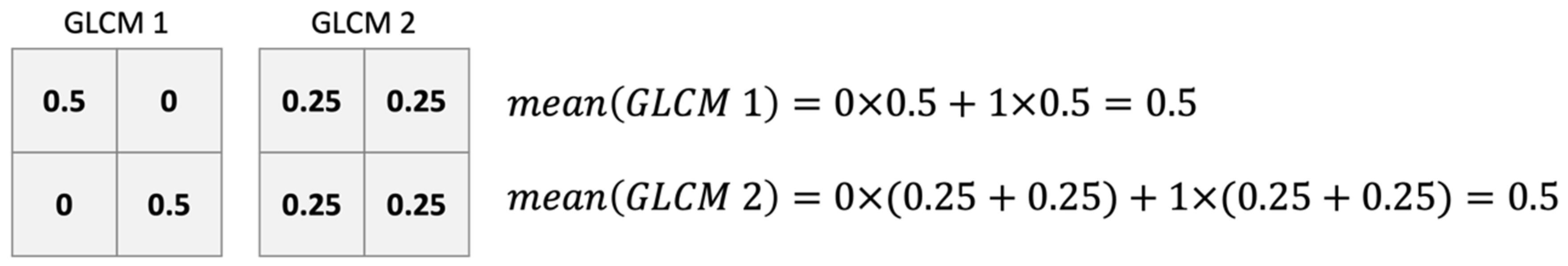
Even though most studies utilized the summary statistics of GLCMs (usually referred to as Haralick features) for subsequent classification applications, we argue that GLCMs with identical summary statistics may possibly possess distinct structures upon revisiting the structure of the GLCM. This implies that selecting representative summary statistics for the GLCM could be pivotal for successful classification. While it is possible to address this by selecting multiple summary statistics simultaneously by incorporating the standard deviation of the GLCM, a broader perspective suggests the direct utilization of the GLCM itself. Considering the inherent risk of information loss associated with any summary statistics, relying solely on the complete probability distribution might best represent all facets of data characteristics. Several methods exist for calculating the empirical probability distribution.

On the other hand, the selection of machine learning models was also a critical issue, which may greatly affect the accuracy of the final prediction result. Previous work includes a comprehensive review about the machine learning or deep learning techniques applied to predict field images obtained from satellites or UAVs. Deep learning models based on Convolution Neural Network (CNN) technology have achieved good accuracy and become the most widely used algorithms [16]. However, other algorithms might be utilized with different considerations. For example, SVM might have higher performance on some occasions [3,16,17]. Classification and regression tree (CART) and other conventional decision tree-based models were easy to interpret with tree-diagram structures [16]. The models based on ensemble learning, such as Extreme Gradient Boosting (XGBoost), have started to attract more attention due to their exceptional performance in complex systems [16,18].

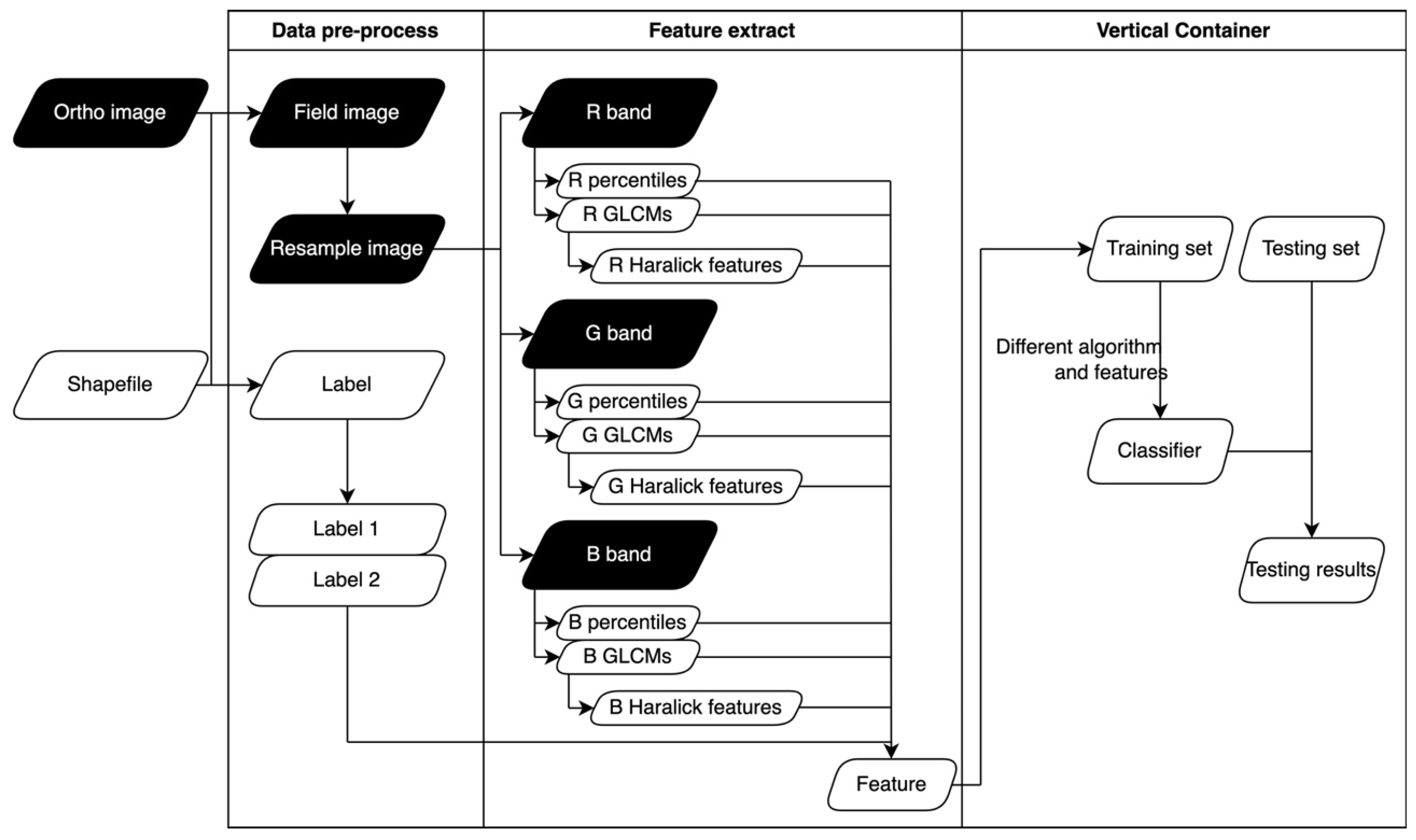
Continuing the above argument, this study proposes to use the entire GLCM empirical distribution as the characteristics of the field to classify the fields. Our study used multitemporal visible-light RGB images taken in agricultural areas of Taiwan and captured by UAV. Since the spectral information that RGB images can provide is less than that of multispectral images, we wish to combine the texture and spectral features to extract more information from the images. A GLCM-based feature extraction process is developed in this study, and the effects of using a GLCM versus Haralick features as additional features were examined for the task of feature recognition. This study also evaluates the performance of three algorithms, CART, SVM, and XGBoost, in field classification with the selected features.

2. Materials and Methods

2.1. Image and Label Data Acquisition

All aerial orthoimages in this study were provided by GEOSAT Aerospace & Technology Inc., Tainan, Taiwan. in Tagged Image File (.tif) Format with GPS coordinates information. Figure 1 shows the study area in this research; the images were obtained in Tainan City and Chiayi County in Taiwan, which covers a major agricultural area of Taiwan. These images were taken at specific dates in December 2019 (2019/12), March 2020 (2020/03), and June 2020 (2020/06); the cover area of the three images was 14,537 ha, 2850 ha, and 5933 ha, respectively. The UAV was equipped with Sony A7R2 (for 2019/12) and A7R3 (for 2020/03 and 2020/06) RGB cameras with a Zeiss Loxia F2.8/21 mm lens and flew at 125–150 m in height. These raw aerial images were processed into orthoimages by the GEOSAT GeoCCP platform [19]. The orthoimages used a ground sample distance (GSD) of 5.18, 4.32, and 3.78 cm, respectively. A total of 10 orthoimages were used in this study, and the file size of all orthoimages was about 980 GB. Well-trained agricultural investigators recorded the location and the category of land use or crop of each field in the study area and created the ground truth shapefile (.shp format) in QGIS [20].

In this study, we selected seven categories of field types, which were Rice, Bean, Fruit, Facility, Maize, Sugarcane, and Aqua, as the research targets (

Table 1. Number of fields for each category on 2019/12, 2020/03, and 2020/06.

Category	Date			Total
	2019/12	2020/03	2020/06
Rice	30	533	194	757
Bean	167	214	74	455
Fruit	65	57	72	194
Facility	168	93	118	379
Maize	1980	423	431	2834
Sugarcane	148	41	50	239
Aqua	2512	280	721	3513
Total	5070	1641	1660	8371

). The number of fields in each category was not balanced. Aqua and Fruit were the categories with the most (3513) and the fewest (194) fields, respectively. Figure 2 and

Table 2. Mean and standard deviation (Sd) for the area of fields for each category (units: ha).

Category	Rice	Maize	Aqua	Bean	Fruit	Facility	Sugarcane
Mean	1.15	2.39	0.70	0.99	0.47	0.91	14.88
Sd	1.29	3.96	1.92	0.62	1.31	3.39	11.68

show the mean and standard deviation of the area per field of each category. Fruit and Sugarcane were the categories with the smallest (0.47 ha) and the largest average area (14.88 ha), respectively.

Figure 3 shows the workflow of this study. It is divided into three parts: data preprocessing, feature extraction, and modeling. All processes were performed in an R environment [21].

2.2. Data Preprocessing

Data preprocessing encompassed various tasks, including data cleaning, image cropping, labeling, resampling, and the segmentation of training and testing sets, among other necessary procedures.

2.2.1. Data Cleaning and Image Cropping

In this study, the fundamental unit of analysis was set at the field level. Each orthoimage covering a large area contained numerous fields. The initial step involved cropping field images from the orthoimages and obtaining individual images for each field. The R environment was utilized to load shapefiles and orthoimages, and fields falling within the specified target categories were selected. Geographic information was extracted from shapefiles and used to crop the corresponding field images. To optimize memory usage and expedite the process, the cropped field images were directly sent to the resampling stage without intermediate storage. The coordination of fields and the processing of orthoimages were executed by the R packages sf and raster [22,23].

2.2.2. Image Labeling

As the orthoimages were acquired on three distinct dates, the crops exhibited varying growth stages, and the appearance at each stage may vary significantly. To account for the temporal effect, two labeling methods were used. The workflow for these two labeling methods is illustrated in Figure 4.

Label 1 combined the images acquired on three different dates. For instance, images of rice fields taken in December 2019, March 2020, and June 2020 were labeled “Rice”; a similar approach was applied to fields belonging to another category. This resulted in a total of seven distinct label categories.

Label 2 represents a labeling approach that combines the temporal effect into the label. Using the same example above, those rice field images were labeled as Rice_1, Rice_2, and Rice_3 to indicate the category and the image acquisition dates at the same time. This method resulted in a total of 21 label categories. To compare the two labeling methods, the detailed labels from label 2 were only employed in model training and prediction. Predicted labels for the same field types but different dates were combined in the final output and the predictions were presented under the original seven categories, the same as the approach in label 1.

2.2.3. Resampling

The UAV orthoimages captured in the field exhibited repetitive patterns, primarily stemming from the planting arrangements employed during crop cultivation and the inherent variations in crop appearances. In the context of rice cultivation in Taiwan, farmers adhere to specific row and column spacings, resulting in a repetitive visual pattern at consistent distances, forming the overall image of a rice field. To address this, an innovative resampling method was introduced, replacing the conventional sliding window approach for generating feature selection inputs. The amplification factor was computed using Equation (1). First, we set the factor $X_c=1000/N_c$, where N_c was the total field number for category c. The value of X_c was then rounded to the nearest integer, with predefined minimum and maximum values set at 1 and 10, respectively.

$$X_c= \mathrm{round}\left[ \max \left(1, \min \left(10,X_c=1000/N_c\right)\right)\right]$$

(1)

Within the area of the ith field image cropped in Section 2.2.1, a set of $X_c$ ‘seed pixels’ was randomly selected. These ‘seed pixels’ were then expanded by 5 m on all four sides to form a square with an area of 100 square meters. Subsequently, all pixels within these determined squares were cropped to generate sample images. The resampling method aimed to capture smaller portions of fields, serving as representative samples for the entire field. This not only saved computing time but also equalized the number of fields in each category through the amplifying factor. To enhance efficiency, the resampled square images were directly sent to the feature extraction stage without storage, aligning with the previously stated rationale.

2.3. Feature Extraction

The resampling images from Section 2.2.3 were used to extract image features, including the 0–100% percentiles and GLCM vectors of the R, G, and B bands. To determine the difference between using GLCM vectors and the Haralick features, which are statistics derived from a GLCM, the Haralick features were also extracted for further comparison.

2.3.1. GLCM Calculated

The (i, j)th element of the $K\times K$ GLCM, denoted as $G_{dist}^{\theta }$, was calculated as follows under the predetermined parameters of distance, dist, and angle, $\theta$ (

Table 3. Combinations of angle ($\theta$) and distance used in this study.

Angle, θ (°)	cos(θ)	−sin(θ)	Distance, dist
0	1	0	1
45	$1/\sqrt{2}$	$-1/\sqrt{2}$	$\sqrt{2}$
90	0	−1	1
135	$-1/\sqrt{2}$	$-1/\sqrt{2}$	$\sqrt{2}$

).

First, one finds the specific neighboring pixel (m, n) according to dist and $\theta$ by letting

$$m=x+dist\times cos\left(\theta \right),\mathrm{and}n=y+dist\times \left(-sin\left(\theta \right)\right).$$

(2)

Then the (i, j)th element of the GLCM, denoted as $G_{dist}^{\theta }\left(i,j\right)$, can be determined by

$$G_{dist}^{\theta }\left(i, j\right)=\#\left[L\left(x,y\right)=i,L\left(m,n\right)=j\right] \mathrm{for} all (\mathrm{x}, \mathrm{y}), \mathrm{or}$$

$$G_{dist}^{\theta }\left(i,j\right)=\sum _{\left(x,y\right)}I\left(L\left(x,y\right)=i,L\left(m,n\right)=j\right),$$

(3)

where # indicates the number of pixel pairs that satisfy the matched gray levels. Let L(x, y) = i (i = 1, …, K) be the gray levels of the pixel at position (x, y);$I\left(\mathrm{E}\right)=1,\mathrm{if}\mathrm{event}\mathrm{E}\mathrm{is}\mathrm{satisfied};0,\mathrm{otherwise}.$ Figure 5 shows an example of turning a gray-level image into a GLCM. There are three occurrences of the number 4 to the right (dist = 1, and angle = 0) of the 1 in the gray-level image matrix. Consequently, the (1,4)th element of the GLCM has been recorded as 3. Figure 6 illustrates an example of the pixel in the image corresponding to different angles and distances in the GLCM. Similar transformations were applied to all combinations of (angle, distance) as listed in Table 3.

GLCMs with identical summary statistics may possibly possess distinct structures upon revisiting the structure of the GLCM. Figure 7 illustrates an example where two different GLCMs have the same mean value, even though the two matrices are distinct. To simplify calculations and facilitate field information analysis for prompt decision-making, we flattened the GLCM matrix into a vector (GLCMv) for presentation of the difference in GLCM distribution. When presenting a GLCM by its row vectors, $G_{dist}^{\theta }={\left({\mathit{v}}_1,{\mathit{v}}_2,\cdots ,{\mathit{v}}_K\right)}^T$. Then the $K^2\times 1$ GLCMv is defined as ${\left(v_1^T,v_2^T,\cdots ,v_K^T\right)}^T.$

2.3.2. Extraction of Image Features: Percentiles, GLCMv, and Haralick Features

The original brightness levels of each band in the images ranged from 1 to 256. For each band, percentiles from 0% to 100%, with a 1% increment of the original brightness ranging from 1 to 256, were computed. When computing GLCMv, the brightness levels of each band were reduced from 256 to 8, equally spaced to reduce the number of potential combinations. The resulting eight-level grayscale underwent GLCMv calculation at 0°, 45°, 90°, and 135° angles. The feature sets of the three bands from the same resampling image were combined with the complete image feature sets. As a result, each resampling image generated 1071 features (color: 101 percentiles × 3 bands = 303; GLCMv: 64 combinations × 4 angles × 3 bands = 768).

For additional comparison, the GLCM of each angle was utilized to calculate the mean and variance, which are commonly used Haralick features, by Equations (4) and (5) [3,11]. Consequently, each resampling image obtained a total of 24 Haralick features (2 statistics × 3 bands × 4 angles). In this study, the R package agrifeature was employed to compute the GLCM [24].

$$Mean \left(\mu \right)={{\displaystyle \sum }}_{i=0}^{K-1}{{\displaystyle \sum }}_{j=0}^{K-1}ip\left(i,j\right)$$

(4)

$$Variance={{\displaystyle \sum }}_{i=0}^{K-1}{{\displaystyle \sum }}_{j=0}^{K-1}{\left(i-\mu \right)}^{2}p\left(i,j\right)$$

(5)

where p(i, j) = $G_{dist}^{\theta }\left(i, j\right)/$[K(K − 1)]; the proportion of the (i, j)-pair occurrence.

2.4. Modeling Algorithms and Testing Metrics

This study employed three common supervised classification algorithms—CART, SVM, and XGBoost—to construct classifiers. To ensure a fair comparison, default parameters were utilized for all three methods, and the data was divided into 70% for training and 30% for testing. In the CART algorithm, the default values of the two parameters, minsplit and complexity (cp), were set as 20 and 0.01, respectively. For the SVM algorithm, we used a radial kernel, and the two parameters, gamma and cost, were given the values 1/(number of features) and 1, respectively. In the XGBoost algorithm, since the prediction objective was multiclass, the parameter objective was set to multi:softmax, and the parameters nround, max_depth, and eta were set to 500, 0.1, and 15, respectively, with reference to the number of data points and the number of features. The R packages rpart, e1071, and XGBoost were employed to develop the CART, SVM, and XGBoost multiclass classification models [25,26,27].

Throughout the model training phase, the elapsed time for training was systematically recorded and treated as a performance metric. Evaluation of fully trained models involved predicting the test set and computing the overall accuracy (OA) and testing time, using the formula provided in Equation (8). Given the uneven distribution of testing samples across categories, a multicategory confusion matrix and balanced accuracy were employed to assess performance in each category, as outlined in Equations (6)–(9). The training and testing were conducted on a personal computer featuring an i7-10700 CPU running at 2.90 GHz, 32 GB RAM, and Windows 10 Enterprise Edition. The confusion matrices and evaluation metrics were computed using the R package caret [28].

$$Overall accuracy \left(OA\right)=\frac{True positive+True negative}{All}$$

(6)

$$recall=\frac{True positive}{True positive+False negative}$$

(7)

$$specificity=\frac{True negative}{True negative+False positive}$$

(8)

$$Balance accuracy=\frac{recall+specificity}{2}$$

(9)

3. Results

3.1. Feature Extraction

Table 4. Mean values of the 0%, 50%, and 100% percentiles of the R, G, and B bands.

Category	R			G			B
	0%	50%	100%	0%	50%	100%	0%	50%	100%
Overall	33.29	83.88	126.03	35.76	86.06	125.98	25.29	69.78	110.71
Aqua	23.20	38.93	56.92	27.58	43.77	60.96	25.01	39.95	57.39
Bean	49.95	107.17	146.84	49.26	103.83	140.86	26.37	75.71	115.96
Facility	37.22	107.56	167.64	38.37	110.22	169.58	40.79	112.27	170.42
Fruit	18.77	90.12	154.88	22.13	93.96	152.80	18.00	76.94	137.63
Maize	27.59	78.75	126.06	32.38	84.93	129.27	21.42	64.00	108.42
Rice	38.68	85.92	117.50	42.41	86.56	117.80	22.58	64.54	102.67
Sugarcane	35.59	102.72	153.18	35.03	100.58	149.45	24.23	81.63	127.20

shows the percentiles of the R, G, and B bands for each category, and

Table 5. The time cost of extracting features in each image date and category (Unit: seconds).

Category	Date			Total
	2019/12	2020/03	2020/06
Rice	156.59	3930.27	7498.01	11,584.87
Bean	610.2	2854.04	1617.89	5082.13
Fruit	379.72	970.42	5042.93	6393.07
Facility	617.16	1325	6169.03	8111.19
Maize	2169.63	1219.09	2823.33	6212.05
Sugarcane	345.37	1047.59	3289.62	4682.58
Aqua	2694.87	1771.32	7427.65	11,893.84

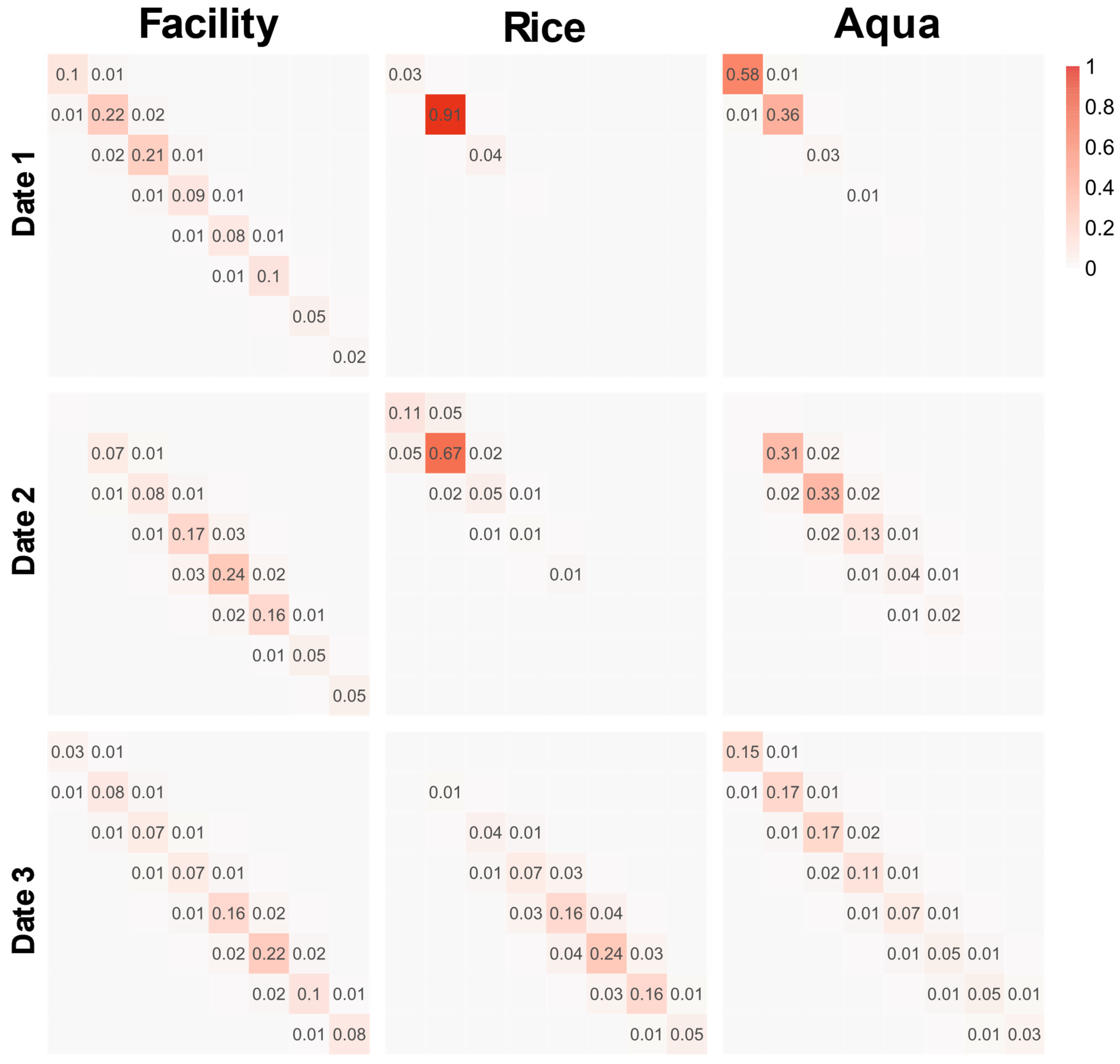
shows the time cost of extracting features in each image date and category. Due to the many percentiles and combinations of bands and angles, only the 0%, 50%, and 100% percentiles for each category and band are shown. Figure 8 shows the GLCM for Facility, Rice, and Aqua on 2019/12, 2020/03, and 2020/06. Due to the vast number of possible combinations of angles, dates, bands, and categories, the plot only displays the average GLCM for all four angles and three bands. Additionally, only three categories deemed significant for discussion have been selected for display.

The values of the R and G bands shown in Table 4 were similar, with the differences at the three percentiles being 2.47, 2.18, and 0.05. However, the values of the B band were relatively lower, and the maximum differences to the other two bands at each percentile were 8, 14.1, and 15.32. Nevertheless, such a relationship does not necessarily exist when observing each category. For example, the 0% percentile values of Aqua were 23.2, 27.58, and 25.01, where the G band had the highest value. However, the 100% percentile values of Facility were 167.64, 110.22, and 170.42, where the R band had the highest value. In addition, certain relationships existed among the percentile values of each category. For example, the 100% percentile values of Aqua were 56.92, 60.96, and 57.39, which were all lower than the 100% percentile values of the other categories, which were all higher than 100. Another example was the 100% percentile values of Facility, which were 167.64, 169.58, and 170.42, which were the highest. The percentile value of different categories shows different patterns, and these patterns can be used for classification in a machine learning model.

The GLCM shown in Figure 8 was concentrated on the diagonal line of the matrix irrespective of the category. The main difference among the categories was the concentration trend and the location of the maximum probability obtained. For example, on 2019/12, the GLCM of Rice showed a high concentration at (2, 2), while the other two categories displayed a more scattered pattern. In addition, the GLCM of the same category may vary considerably at different times. Again, in the case of Rice, for example, there is an obvious difference in the GLCMs for the three dates. In contrast, there is not much difference in the GLCMs for Facility on the three dates.

3.2. Overall Classification Results

Table 6. Overall classification results of each classifier, including the OA, training time spent, training CPU time spent, and testing time spent.

	Label 1			Label 2
	CART	SVM	XGBoost	CART	SVM	XGBoost
OA	0.527	0.731	0.808	0.562	0.756	0.820
Training time (s)	19.22	590.67	140.65	28.81	402.47	259.13
Training CPU time (s)	19.22	590.67	1962.22	28.81	402.47	3109.56
Testing time (s)	0.07	37.28	0.08	0.09	36.77	0.11

shows the OA and the time spent on model training and testing of six classifiers constructed by the combination of three algorithms and two labeling methods. Because the XGBoost algorithm allows training of the models by parallel computing, the CPU time spent on training, which means the sum of computing resources consumed by each CPU core, was also recorded.

The relation among the overall classification accuracies of the six classifiers was XGBoost with label 2 > XGBoost with label 1 > SVM with label 2 > SVM with label 1 > CART with label 2 > CART with label 1. The classifier with the XGBoost algorithm and label 2 had the highest OA of 0.82, followed by the classifier with the XGBoost algorithm and label 1. The worst-performing classifier used CART and label 1 and had an OA of only 0.527.

In terms of time spent on model training, the classifier with the CART algorithm and using label 1 took 19.22 s, which was the shortest time. In comparison, the classifier with the SVM algorithm and using label 1 took 590.67 s, which was the longest time. For the two tree-based algorithms CART and XGBoost, when label 2 was used, because the number of categories increased, the training time also increased by about 50–80%. However, for the SVM classifier, when using label 2, the training time was reduced by 30%, which showed a different trend from the other two classifiers. In terms of CPU time spent on training, the classifier with XGBoost and label 2 consumed the most computing resources, taking 3109.56 s.

In terms of time spent on model testing, the difference between the classifiers with the same algorithm but using different labels was relatively minor. The SVM classifiers took 37.28 and 36.77 s for the two labels. For the CART and XGBoost classifiers, the testing time consumed was relatively lower and was about 0.1 s, which was about 0.2% of what the SVM classifiers took.

3.3. Classification Results for Each Category

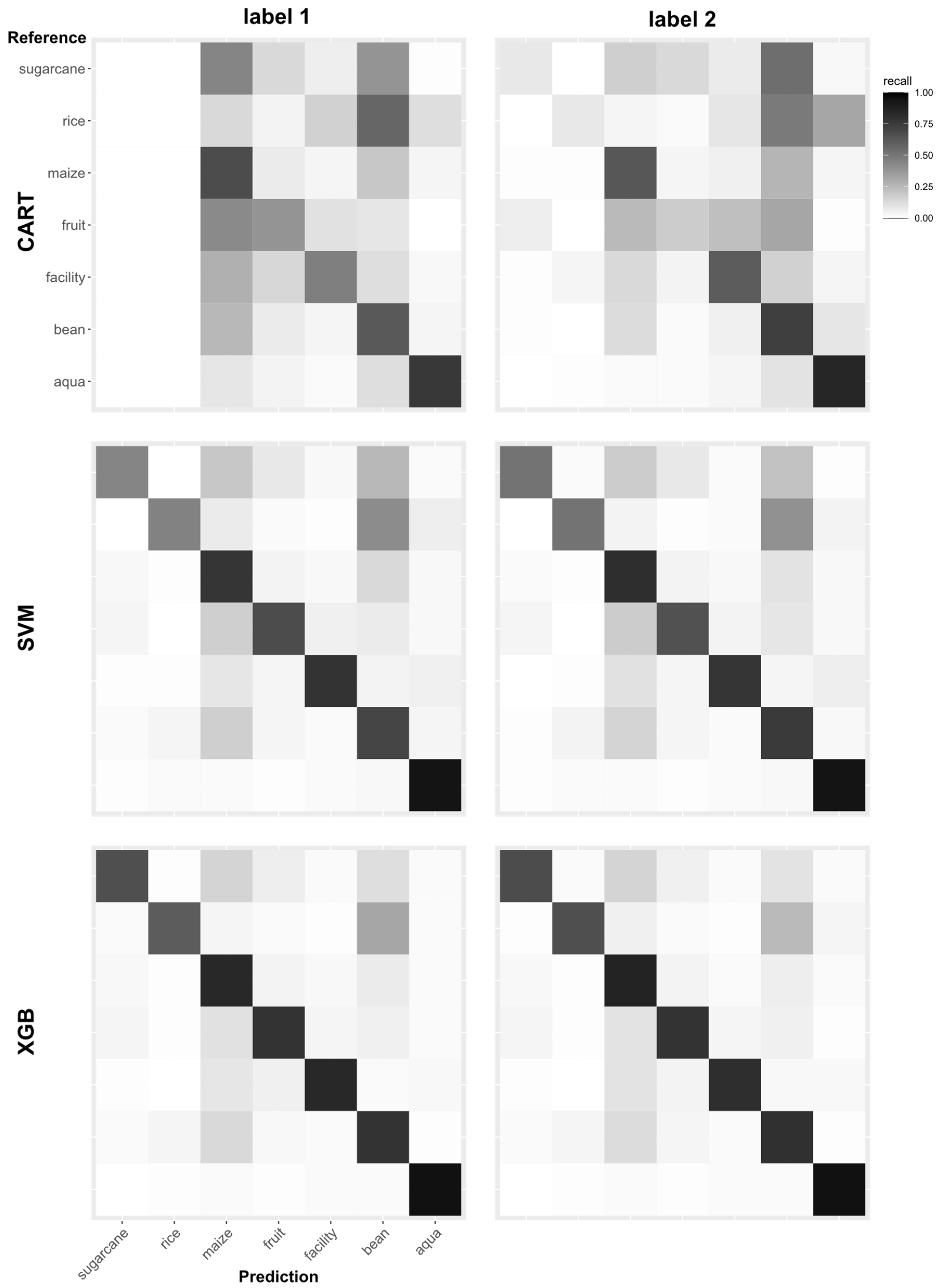
Figure 9 and

Table 7. Testing balance accuracy of each classifier for each category.

Label	Model	Aqua	Bean	Facility	Fruit	Maize	Rice	Sugarcane
1	CART	0.86	0.71	0.70	0.66	0.71	0.50	0.50
	SVM	0.95	0.80	0.88	0.81	0.83	0.71	0.71
	XGBoost	0.96	0.85	0.90	0.87	0.88	0.81	0.83
2	CART	0.89	0.74	0.77	0.57	0.76	0.54	0.53
	SVM	0.95	0.82	0.88	0.82	0.85	0.73	0.76
	XGBoost	0.97	0.86	0.90	0.89	0.88	0.82	0.84

show the testing results of the six classifiers by confusion matrix and accuracy, respectively. Due to mismatch in the size of testing data across categories, balance accuracy was used in Table 7 for more accurate evaluation.

The confusion matrixes show that none of the data were predicted in the categories Rice and Sugarcane of the classifier with CART and label 1, which means that the classifier ignores these two categories during model training and misclassifies those data into other categories. Although those two categories were predicted by the classifier with CART and label 2, it does not achieve comparable accuracy to the other categories. In the classification results of the classifiers with SVM and XGBoost, the problem that some categories were ignored was not observed. The confusion matrixes of XGBoost were highly concentrated on the diagonal line, which indicates that the classification was performed well. The results of each category for the same classifier were different in the confusion matrixes. For example, Aqua showed high accuracies for all classifiers while Rice and Maize performed poorly.

Table 7 also shows that the balance accuracy of Aqua for the classifier with XGBoost and label 2 reaches the highest value of 0.97, and the classifier with XGBoost and label 1 reaches the second-highest value of 0.96. The categories Rice and Sugarcane with CART and label 1 both had the lowest balance accuracy of 0.5, which means that all of the data belonging to Rice or Sugarcane are predicted as other categories, as in the confusion matrix. When observing results within a category, the classifiers with the XGBoost algorithm obtained the most accurate prediction results, followed by those with SVM and CART. For each classifier, model building using the XGBoost algorithm obtained the closest balance accuracy among the categories, where the maximum difference between the best and the worst performance was only 0.15. In contrast, the classifier with the CART algorithm had the largest accuracy difference among the categories, which reached 0.36.

Irrespective of the algorithm applied, the OA of the classifiers trained with label 2 was better than that of classifiers trained with label 1, and the testing OA was improved by 1–5%. For the classifiers with the XGBoost and SVM algorithms, label 2 improved the balance accuracy by 1–5% for each category. However, for the classifiers with the CART algorithm, label 2 reduced the accuracy of Fruit by 9% but improved the accuracies of the other categories by 3–7%.

3.4. Classification Results for GLCMv, Haralick Feature, and Percentile

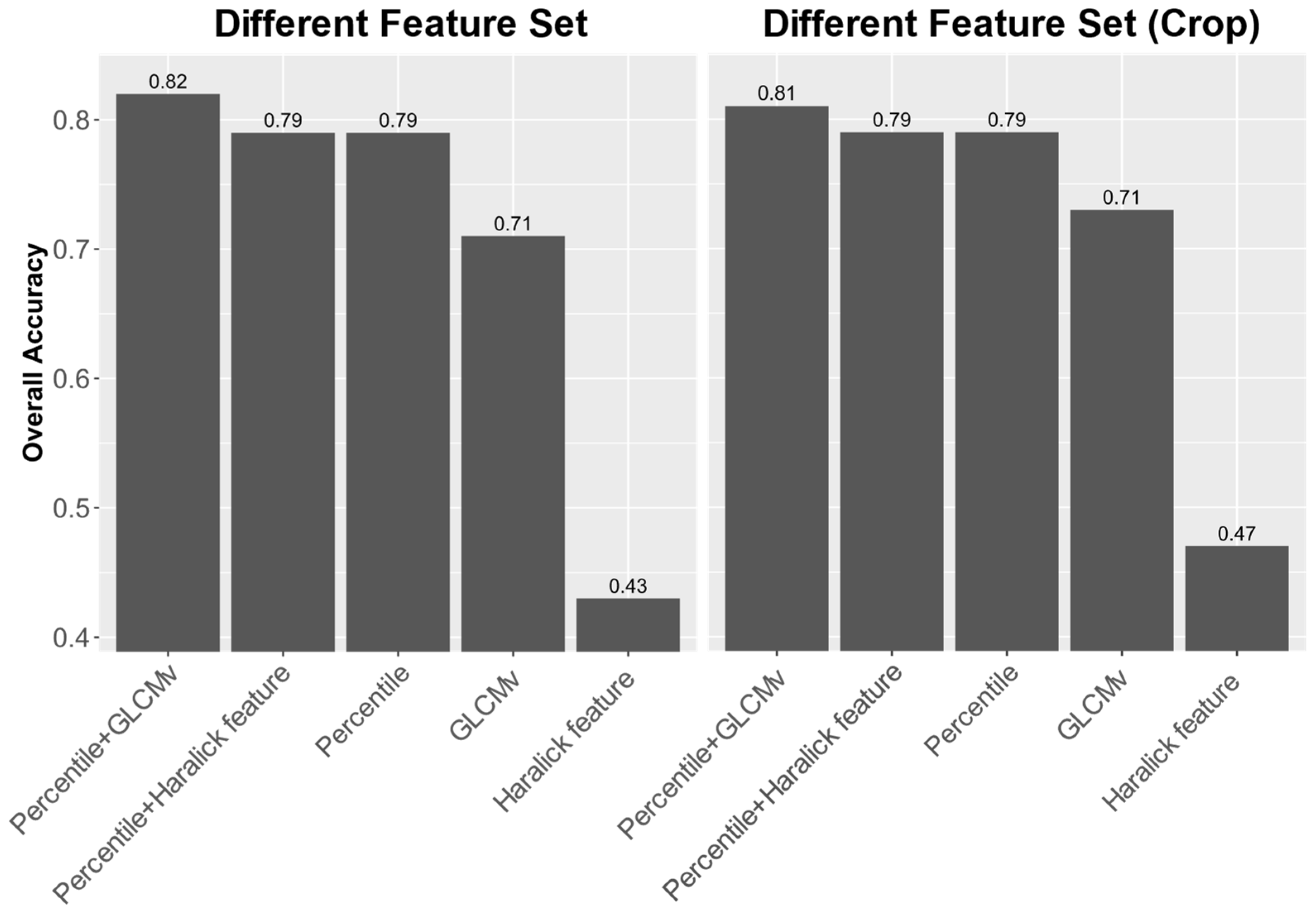
The left part of Figure 10 shows the testing accuracy when different feature combinations were used. As discussed in Section 2.3.2, the percentiles, GLCMv, and Haralick features (mean and standard deviation of the GLCM) of each band were extracted and combined differently. Five feature sets, namely Haralick feature, GLCMv, percentiles, percentiles + Haralick feature, and percentiles + GLCMv, were used to test their contribution to the classification problem. The algorithm and label used in the test were XGBoost and label 2, respectively, to ensure the best performance. The highest accuracy was obtained using percentiles + GLCMv, the same as the result in Section 3.2, with a total accuracy of 0.82. The classifiers using only percentiles and percentiles + Haralick feature showed the second-highest accuracy (0.79), while the accuracies of using only GLCMv and Haralick feature were 0.71 and 0.43, respectively. The result shows an improvement of about 3.6% on overall accuracy when adding GLCMv to the classifier. We used McNemar’s test [29] to compare the prediction results of percentiles, and percentiles + GLCMv. The p-value was less than 10⁻¹⁵, indicating a significant difference between the two results.

To understand the effect of features on the classification of different crops, the categories Aqua and Facility, which did not belong to crops, were removed to observe the classification accuracy of different crop types only. The results are shown in the right part of Figure 10. The accuracy trend among the feature sets was the same as in the left part of the figure, which means that the classification results were not highly affected by Aqua and Facility, and this system can perform well on different types of crops. The OA of using the feature set percentiles + GLCMv dropped slightly to 0.81, while the accuracies of using only the GLCMv and Haralick feature increased a little to 0.73 and 0.47, respectively. The percentage of improvement and the result of McNemar’s test were the same as above.

4. Discussion

4.1. Resampling

Resampling is crucial for data preprocessing. It balances the sample size and allows direct GLCM vector extraction. Two key parameters were the maximum amplification factor (Xc) and the size of the resampled square image.

We selected a larger resampled image size to account for the variation in field types. This ensures that the image can cover multiple objects on the ground, even if there is a significant difference in size. Based on the field area listed in Table 2, even the most minor field type, Fruit, has an average area of 0.47 ha, so a size of 100 square meters does not occupy a significant portion of the field image. This allows us to create multiple resampled images in the same field. According to Table 1, the number of fields in each category varied greatly, and the smallest categories were Rice in 2019/12, Sugarcane in 2020/03, and Sugarcane in 2020/06, with only 30, 41, and 50 fields, respectively. This limited number of fields may make it challenging to train the machine learning models, and there is also a risk of encountering an unbalanced size among categories. To minimize overlap and increase the data size for the minor categories, we set the maximum amplification factor to 10. Based on the GSD of the images, it can be inferred that a 100-square-meter area would contain tens of thousands to hundreds of thousands of pixels on different orthoimages. This quantity of pixels was seen as a small size for image analysis, especially for the relatively simple feature extraction methods. Therefore, it is not a computationally intensive event even though several resampled images were computed. However, it is important to note that the parameters used for this process should be adjusted based on the GSD of the image, field size, different field types, computational resources, and other relevant factors.

Table 8. The size of resampled images for each category on 2019/12, 2020/03, and 2020/06.

Category	Date			Total
	2019/12	2020/03	2020/06
Rice	300	1066	970	2336
Bean	1002	1070	740	2812
Fruit	650	570	720	1940
Facility	1008	930	944	2882
Maize	1980	846	862	3688
Sugarcane	1036	410	500	1946
Aqua	2512	1120	721	4353

presents the number of resampled images for each field type on three different dates after resampling. It shows that this method expands the data size of the minor category, resulting in a minimum image size of 300, which provides more images for the training and testing of the machine learning algorithm. At the same time, by calculating the amplification factor of different categories, the difference in the number of images between categories was also reduced. The difference in the total number of images between the categories with the smallest and the largest number of images was only 2.24 times.

4.2. Percentile and GLCM

The data presented in Table 4 reveal distinct differences between percentiles across categories. For instance, Aqua’s percentiles were comparable to other categories at lower percentiles but became lower than others at the 50th and 100th percentiles, irrespective of the bands. In contrast, Facilities exhibit superiority over other categories only at the 100th percentile. This underscores the importance of employing diverse percentiles as features, as their combination may yield more effective categorization than relying solely on mean or median values. Therefore, variations in percentiles across different categories suggest the suitability of percentiles as color indices.

As indicated in the results, the concentration and trend of GLCMs varied not only among different categories but also over time. For instance, in the case of Rice, the three dates span from seedling planting to ripening, leading to significant differences in the rice field images. We attribute the variation in GLCMs during these dates to this temporal progression. While Facilities, being non-plant entities, exhibited minimal changes over the three dates, Aqua, also non-plant, displayed substantial variations. We attribute this difference to discrepancies in the locations of the three images and the inherent diversity in Aqua images at those locations. Consequently, the variations in GLCM may arise from changes within the category over time or regional disparities.

4.3. Comparison among the Algorithms

In terms of overall accuracy, both XGBoost and SVM produced classification results with overall accuracies as high as 75.6% and 82%, while CART only achieved 52.6% accuracy. Previous studies have shown that the use of SVM combined with GLCM can achieve good classification results, and the results of this study show the same trend, indicating that SVM can effectively capture important information from complex image features [3,14]. As can be seen in a previous review, when the number of features is larger or the features become more complex, CART may not be able to capture the critical information in the data, and thus, the classification performance would be lower than that of other algorithms [16]. In this study, due to the complexity of color and texture features, CART was disadvantaged in handling such a problem compared to more complex algorithms such as SVM and XGBoost.

Comparing all three algorithms, the XGBoost algorithm outperformed others in all three metrics: overall accuracy, training time, and testing time. XGBoost demonstrated efficient prediction capabilities for new data within a short timeframe. In previous studies, RF was used as an example to show that the tree-based ensemble learning algorithm can effectively use the structure of multiple trees to capture important features when combined with the GLCM, and can utilize the voting mechanism to get better results [3,14]. The same reason may also explain why XGBoost, which is also a tree-based ensemble learning algorithm but more powerful, demonstrates such good accuracy. The observed testing time trends align with findings in previous studies across various fields, suggesting XGBoost’s suitability for agricultural image recognition [16,30,31]. Another notable advantage of XGBoost is its capacity for accelerated training through parallel computing on platforms with multiple CPU cores. While XGBoost consumes the most CPU time, indicative of substantial computing resources, parallel computing significantly reduces the training times, enhancing efficiency. However, the effectiveness of parallel computing depends on the computing platform’s number of CPU cores and whether GPUs are utilized. In scenarios with limited resources or single-core computing platforms, training times for XGBoost may exceed those of other algorithms.

When assessing classifier performance within each category, it is evident that both classifiers utilizing the CART algorithm exhibit lower accuracy in Rice and Sugarcane. This phenomenon, where a classifier tends to overestimate the main category with a large sample size or minimal intragroup variation while neglecting minor categories, is more likely in datasets characterized by unequal sample sizes or a substantial number of categories [32]. To mitigate the oversight of minor categories, modifications to the algorithm’s loss function or evaluation method can be considered to increase the associated penalty or by adopting ensemble learning-based algorithms [32,33,34,35]. SVM employs a multiclass classifier formed by voting on binary classifier results, reducing the tendency to overlook minor categories through classifier ensembling [17]. XGBoost, an ensemble learning algorithm, aggregates results from multiple classifiers, akin to the multiclass SVM mentioned earlier, effectively preventing the neglect of minor categories. This elucidates why XGBoost exhibits high accuracy in classifying multiclass image datasets.

4.4. The Effect of GLCM and Haralick Features

The outcomes reveal that the percentiles of images representing color features contribute significantly to image classification, whether for all categories or exclusively for crops. Emphasizing color features in the classifier yielded robust performance during testing, aligning with findings from prior studies and underscoring the importance of spectral information [3,36]. Combining the dataset with GLCMv and percentiles resulted in an improved accuracy of approximately 2 to 3 percentage points. When comparing GLCMv and Haralick features, employing only a single texture feature from GLCMv led to a classification accuracy of 28 and 25 percentage points higher than that achieved with Haralick features in two distinct scenarios. This suggests that the direct utilization of GLCMv imparts more information than Haralick features, and proficient machine learning algorithms adeptly capture more information from these features. Interestingly, when both types of texture features were added to color features, accuracy improved only with the inclusion of GLCMv, signifying that Haralick features did not provide supplementary information to a model already equipped with information from color features. The proposed resampling method for feature extraction obviates the need to calculate texture features and generate feature maps, as required by sliding window methods. Moreover, it enables the direct use of GLCMv from each field as features, thereby enhancing the provision of valuable information.

4.5. Temporal Effect

To compare the impact of adding temporal effects on the data labels, we calculated the Within-group Sum of Squares (WSS) for two sets of labels. The mean value of each feature for every category was represented as the cluster center, and the Euclidean distance was calculated. Since each category in Label 1 corresponded to three categories in Label 2, we aggregated the three WSS values for the same category to derive the WSS for Label 2.

In contrast to label 1, label 2 regroups the categories by the imaging date to reduce variability.

Table 9. WSS of each category under two different labeling methods and the improvement in WSS and the OA using label 2.

	Aqua	Bean	Facility	Fruit	Maize	Rice	Sugarcane
Label 1	807,313	2,364,385	1,333,897	741,067	1,961,822	778,614	735,664
Label 2	649,441	1,626,266	1,183,913	667,866	1,754,380	267,928	690,059
WSS improvement	2%	31%	11%	1%	11%	66%	6%
Accuracy improvement	1%	1%	0%	2%	0%	1%	1%

shows the WSS for each category under label 1 and label 2, the reduction in WSS using label 2, and the enhancement in Overall Accuracy (OA) for the XGBoost classifier. Notably, substantial differences in WSS values exist among categories, with Bean having the largest WSS at 2,364,385 and Sugarcane the smallest at 735,664 when using label 1. Label 2 diminishes the WSS due to an increase in the number of group centers in each category. Label 2 decreased the WSS of Rice and Bean by 66% and 31%, respectively. The decreasing WSS indicates the difference in features across three photo dates, and the difference is likely due to the changes in crop appearance throughout different growth stages. The information on the imaging date leads to a WSS reduction, and it likely contributes to the observed improvement in testing OA. This reduction in WSS also explains why classifiers employing SVM can train faster using label 2, as a smaller WSS could make the algorithm’s identification of support vectors more efficient and expedite the training process [37].

5. Conclusions

In this investigation, we employ high-resolution and multitemporal visible-light RGB UAV imagery for analysis. By integrating the texture and color features and utilizing machine learning classification algorithms, we develop an effective multiclass classification model to discern Taiwan’s fragmented and diverse agricultural lands. The most successful model attains an overall accuracy of up to 82%. Exploiting the repetitive patterns within the field images allows us to adapt the feature extraction process through resampling, addressing the unequal number of samples, and facilitating the use of GLCMv as a texture feature.

Advancements in machine learning algorithms have enabled us to achieve enhanced classification accuracy using the same features. The XGBoost algorithm, rooted in ensemble learning, surpasses its traditional CART or SVM counterparts in accuracy while exhibiting shorter training times and rapid recognition capabilities. Regarding image features, we utilize the percentiles of the three RGB bands as color features for distinguishing various land-use types. Examining texture differences among land use types reveals that employing GLCMv as the texture feature yields more informative results, leading to improved classification accuracy compared to using the Haralick feature. Leveraging more powerful machine learning models and features containing richer information, such as GLCMv, while entrusting the task of information extraction to the machine learning model, is a preferable choice for enhancing model accuracy.

Concerning the temporal effect, our observations indicate that temporal disparities in crop types were crucial in influencing classification outcomes. This underscores the need for a more nuanced consideration of temporal differences in future analyses, where temporal variations in crop imagery will be a focal point in our ongoing research. Moving forward, we aim to delve into temporal and spatial variations more comprehensively. Simultaneously, we aspire to leverage the features of GLCMs to furnish analyzable information on texture differences that can serve as indices for tracking such variations.

References

1. Chen, P.-C.; Chiang, Y.-C.; Weng, P.-Y. Imaging using unmanned aerial vehicles for agriculture land use classification. Agriculture 2020, 10, 416. [Google Scholar] [CrossRef]
2. Böhler, J.E.; Schaepman, M.E.; Kneubühler, M. Crop classification in a heterogeneous arable landscape using uncalibrated UAV data. Remote Sens. 2018, 10, 1282. [Google Scholar] [CrossRef]
3. Kwak, G.-H.; Park, N.-W. Impact of texture information on crop classification with machine learning and UAV images. Appl. Sci. 2019, 9, 643. [Google Scholar] [CrossRef]
4. Shen, X.; Teng, Y.; Fu, H.; Wan, Z.; Zhang, X. Crop identification using UAV image segmentation. In Proceedings of the Second Target Recognition and Artificial Intelligence Summit Forum, Shenyang, China, 28–30 August 2019; pp. 480–484. [Google Scholar]
5. Shi, G.; Du, X.; Du, M.; Li, Q.; Tian, X.; Ren, Y.; Zhang, Y.; Wang, H. Cotton Yield Estimation Using the Remotely Sensed Cotton Boll Index from UAV Images. Drones 2022, 6, 254. [Google Scholar] [CrossRef]
6. Fu, L.; Duan, J.; Zou, X.; Lin, G.; Song, S.; Ji, B.; Yang, Z. Banana detection based on color and texture features in the natural environment. Comput. Electron. Agric. 2019, 167, 105057. [Google Scholar] [CrossRef]
7. Tian, D. A review on image feature extraction and representation techniques. Int. J. Multimed. Ubiquitous Eng. 2013, 8, 385–396. [Google Scholar]
8. Herzig, P.; Borrmann, P.; Knauer, U.; Klück, H.-C.; Kilias, D.; Seiffert, U.; Pillen, K.; Maurer, A. Evaluation of RGB and multispectral unmanned aerial vehicle (UAV) imagery for high-throughput phenotyping and yield prediction in barley breeding. Remote Sens. 2021, 13, 2670. [Google Scholar] [CrossRef]
9. De Swaef, T.; Maes, W.H.; Aper, J.; Baert, J.; Cougnon, M.; Reheul, D.; Steppe, K.; Roldán-Ruiz, I.; Lootens, P. Applying RGB-and thermal-based vegetation indices from UAVs for high-throughput field phenotyping of drought tolerance in forage grasses. Remote Sens. 2021, 13, 147. [Google Scholar] [CrossRef]
10. Yang, N.; Yuan, M.; Wang, P.; Zhang, R.; Sun, J.; Mao, H. Tea diseases detection based on fast infrared thermal image processing technology. J. Sci. Food Agric. 2019, 99, 3459–3466. [Google Scholar] [CrossRef]
11. Haralick, R.M.; Shanmugam, K.; Dinstein, I.H. Textural features for image classification. IEEE Trans. Syst. Man Cybern. 1973, SMC-3, 610–621. [Google Scholar] [CrossRef]
12. Garg, M.; Dhiman, G. A novel content based image retrieval approach for classification using glcm features and texture fused lbp variants. Neural Comput. Appl. 2020, 33, 1311–1328. [Google Scholar] [CrossRef]
13. Hall-Beyer, M. GLCM Texture: A Tutorial v. 3.0, University of Calgary: Calgary, AB, Canada, March 2017.
14. Iqbal, N.; Mumtaz, R.; Shafi, U.; Zaidi, S.M.H. Gray level co-occurrence matrix (GLCM) texture based crop classification using low altitude remote sensing platforms. PeerJ Comput. Sci. 2021, 7, e536. [Google Scholar] [CrossRef] [PubMed]
15. Xiao, Y.; Dong, Y.; Huang, W.; Liu, L.; Ma, H. Wheat fusarium head blight detection using UAV-based spectral and texture features in optimal window size. Remote Sens. 2021, 13, 2437. [Google Scholar] [CrossRef]
16. Benos, L.; Tagarakis, A.C.; Dolias, G.; Berruto, R.; Kateris, D.; Bochtis, D. Machine learning in agriculture: A comprehensive updated review. Sensors 2021, 21, 3758. [Google Scholar] [CrossRef] [PubMed]
17. Chandra, M.A.; Bedi, S. Survey on SVM and their application in image classification. Int. J. Inf. Technol. 2021, 13, 1–11. [Google Scholar] [CrossRef]
18. Sagi, O.; Rokach, L. Ensemble learning: A survey. Wiley Interdiscip. Rev. Data Min. Knowl. Discov. 2018, 8, e1249. [Google Scholar] [CrossRef]
19. GEOSAT Aerospace & Technology Inc. GEOSAT GeoCCP; GEOSAT Aerospace & Technology Inc.: Taipei, Taiwan, 2021. [Google Scholar]
20. QGIS.org. QGIS Geographic Information System; Open Source Geospatial Foundation Project. Available online: http://qgis.org (accessed on 29 March 2023).
21. R Core Team. R: A Language and Environment for Statistical Computing; R Foundation for Statistical Computing: Vienna, Austria, 2019. [Google Scholar]
22. Pebesma, E.J. Simple features for R: Standardized support for spatial vector data. R J. 2018, 10, 439. [Google Scholar] [CrossRef]
23. Hijmans, R.J. Raster: Geographic Data Analysis and Modeling. In R Package Version 3.0-7. Available online: https://cran.r-project.org/web/packages/raster/index.html (accessed on 29 March 2023).
24. Lee, C.-H.; Liu, L.-Y.D. Agrifeature: Agriculture Image Feature. In R Package Version 1.0.3. Available online: https://cran.r-project.org/web/packages/agrifeature/index.html (accessed on 29 March 2023).
25. Meyer, D.; Dimitriadou, E.; Hornik, K.; Weingessel, A.; Leisch, F. e1071: Misc Functions of the Department of Statistics, Probability Theory Group (Formerly: E1071), TU Wien; R Package Version 1.7-9. Available online: https://cran.r-project.org/web/packages/e1071/index.html, (accessed on 29 March 2023).
26. Terry Therneau, B.A. Rpart: Recursive Partitioning and Regression Trees. In R Package Version 4.1.23. Available online: https://cran.r-project.org/web/packages/rpart/index.html (accessed on 29 March 2023).
27. Chen, T.; He, T.; Benesty, M.; Khotilovich, V.; Tang, Y.; Cho, H.; Chen, K.; Mitchell, R.; Cano, I.; Zhou, T.; et al. xgboost: Extreme Gradient Boosting; R Package Version 1.6.0.1. Available online: https://cran.r-project.org/web/packages/xgboost/index.html (accessed on 29 March 2023).
28. Kuhn, M. Caret: Classification and Regression Training. In R Package Version 6.0-94. Available online: https://cran.r-project.org/web/packages/caret/index.html (accessed on 29 March 2023).
29. Agresti, A. Categorical Data Analysis; John Wiley & Sons: Hoboken, NJ, USA, 2012; Volume 792. [Google Scholar]
30. Fan, J.; Wang, X.; Wu, L.; Zhou, H.; Zhang, F.; Yu, X.; Lu, X.; Xiang, Y. Comparison of Support Vector Machine and Extreme Gradient Boosting for predicting daily global solar radiation using temperature and precipitation in humid subtropical climates: A case study in China. Energy Convers. Manag. 2018, 164, 102–111. [Google Scholar] [CrossRef]
31. Liu, J.; Wu, J.; Liu, S.; Li, M.; Hu, K.; Li, K. Predicting mortality of patients with acute kidney injury in the ICU using XGBoost model. PLoS ONE 2021, 16, e0246306. [Google Scholar] [CrossRef]
32. Chicco, D.; Jurman, G. The advantages of the Matthews correlation coefficient (MCC) over F1 score and accuracy in binary classification evaluation. BMC Genom. 2020, 21, 6. [Google Scholar] [CrossRef]
33. Sahare, M.; Gupta, H. A review of multi-class classification for imbalanced data. Int. J. Adv. Comput. Res. 2012, 2, 160. [Google Scholar]
34. Lorena, A.C.; De Carvalho, A.C.; Gama, J.M. A review on the combination of binary classifiers in multiclass problems. Artif. Intell. Rev. 2008, 30, 19–37. [Google Scholar] [CrossRef]
35. Fürnkranz, J. Round robin rule learning. In Proceedings of the Eighteenth International Conference on Machine Learning (ICML 2001), Williams College, Williamstown, MA, USA, 28 June–1 July 2001; pp. 146–153. [Google Scholar]
36. Weisberg, P.J.; Dilts, T.E.; Greenberg, J.A.; Johnson, K.N.; Pai, H.; Sladek, C.; Kratt, C.; Tyler, S.W.; Ready, A. Phenology-based classification of invasive annual grasses to the species level. Remote Sens. Environ. 2021, 263, 112568. [Google Scholar] [CrossRef]
37. De Almeida, M.B.; de Pádua Braga, A.; Braga, J.P. SVM-KM: Speeding SVMs learning with a priori cluster selection and k-means. In Proceedings of the Sixth Brazilian Symposium on Neural Networks, Rio de Janeiro, Brazil, 25 November 2000; Volume 1, pp. 162–167. [Google Scholar]
Figure 1. The study area in this research.
Remotesensing 16 01221 g001
Figure 2. Boxplot for the area of fields for each category (units: ha).
Remotesensing 16 01221 g002
Figure 3. The workflow of this study. Includes three major parts: data preprocessing, feature extraction, and modeling.
Remotesensing 16 01221 g003
Figure 4. Workflow of the two different labeling methods.
Remotesensing 16 01221 g004
Figure 5. An example of turning a gray level image with 5 gray levels (K = 5) into a GLCM.
Remotesensing 16 01221 g005
Figure 6. An example of the pixel in the image corresponding to different angles and distances in the GLCM. The combinations of angles and distances used are the same as in Table 3.
Remotesensing 16 01221 g006
Figure 7. An example of two different GLCMs that have the same mean value.
Remotesensing 16 01221 g007
Figure 8. Results of the GLCM for Facility, Rice, and Aqua on three dates.
Remotesensing 16 01221 g008
Figure 9. Testing confusion matrix for each classifier.
Remotesensing 16 01221 g009
Figure 10. (Left) OA of different feature set combinations. (Right) OA of different feature set combinations when only observing the crop categories.
Remotesensing 16 01221 g010