1. Introduction
Seagrasses are rooted aquatic plants that grow completely underwater and are extremely important for coastal ecosystems. Seagrass meadows accumulate organic carbon at an annual rate of 83 gC m
−2 yr
−1, which is larger than what most terrestrial ecosystems accumulate [
1]. Despite only being a relatively small area of the coastal ocean, they are a significant component of the total carbon burial in the ocean, amounting to a global carbon burial rate of 27∼44 TgC yr
−1 (10–18% of total carbon burial in the ocean) [
2]. A large-scale study investigating Bahamian seagrass carbon stocks and sequestration rates showed that the mapped Bahamian seagrass extent covers an area up to 46,792 km
2, translating into a carbon storage of 723 Mg C and a sequestration rate of 123 Mt CO
2 annually, equaling about 68 times the amount of CO
2 emitted by the Bahamas in 2018 [
3]. Seagrass meadows also provide important ecosystem services. Firstly, seagrass canopies act as filters, meaning organic matter from other sources accumulates in the sediments in the meadows [
4]. Additionally, the plants efficiently remove excess nitrogen and phosphorus from coastal waters [
5]. Furthermore, seagrass ecosystems reduce the water’s exposure to bacterial pathogens and improve water quality [
6]. Finally, seagrasses also provide food and shelter to many aquatic organisms in coastal ecosystems, from tiny invertebrates to large fish, crabs, turtles, marine mammals, and birds. A change in seagrass density and types impacts sea creature habitats and the population of these sea creatures [
7]. For example, in the last decade, the Chesapeake Bay has experienced a shift in seagrass species from eelgrass to widgeon grass due to anthropogenic impacts. This shift results in a seagrass emergence time shift from eelgrass emergence in early spring to widgeon grass emergence in summer. This emergence time shift impacts the population density of species such as blue crabs and black sea bass, which need seagrass habitats when they migrate into the bay during the spring months [
7].
Despite the high economic value provided by the aforementioned ecosystem services, seagrass extent is in global decline due to a range of factors, including alterations in coastal habitats [
8,
9,
10]. Nearshore marine ecosystems are experiencing an increase in human impact which is deteriorating water quality in coastal regions [
9,
11]. Across the globe, there has been a dramatic decrease in seagrass extent due to anthropogenic impacts, which has resulted in the loss of seagrass ecosystem services [
12]. This human activity results in rapidly disappearing seagrass, and about 29% of the known areal extent has disappeared since seagrass areas were initially recorded in 1879. Seagrass meadow area is therefore potentially being lost at an estimated average global rate of 1.5% per year [
8]. A recent study over seven seagrass bioregions at the global scale found an overall 19.1% loss of the total area surveyed since 1880 [
9]. However, the true extent of seagrass loss remains uncertain due to estimates of the global seagrass extent being unknown [
13]. Seagrass losses are expected to continue, emerging as a pressing challenge for coastal management. Active restoration efforts are being conducted in the US [
14,
15], Australia, and New Zealand [
13] with some success. Monitoring the loss and recovery of the meadows globally is critical due to a lack of in situ data.
The decline of seagrass density can lead to fragmentation and potentially permanent habitat loss. As seagrass density decreases, the habitat complexity decreases, meaning seagrass beds are less suitable for many animal life stages, including vulnerable life stages such as juveniles seeking to avoid predation. For example, studies showed juvenile crab density was a positive exponential function of seagrass density at a broad spatial scale in Chesapeake Bay [
16,
17]. Additionally, many marine species, such as dugongs, manatees, and sea turtles, depend directly on these habitats for food [
18]. Seagrass density is also associated with fish abundance [
19] and benthic biodiversity of bacteria and macroinvertebrates [
18]. The faunal community species diversity and richness were significantly higher in high-cover seagrass than in low-cover seagrass, indicating increasing habitat value as density increases [
20]. In essence, maintaining and mapping seagrass density is a priority for conservation efforts.
1.1. Remote Sensing of Seagrass
To date, seagrass is primarily monitored using in situ approaches, including ground surveys and hovercraft-based mapping. However, satellites offer a cheaper and more consistent approach to mapping seagrass distribution at high temporal resolution [
21]. Currently, a range of high-resolution multispectral data is being used to map seagrass meadows [
22]. The success of remote sensing methods is highly dependent on the spatial/spectral resolution of the data and mapping methods. Higher spatial resolution data allows for higher accuracy in mapping seagrass than lower resolution data [
21]. However, high-resolution data often comes at the cost of spatial coverage, as seen in the many local studies using aerial photography to map seagrass meadows [
23,
24]. Due to low spatial coverage, aerial photography is too expensive to be conducted for all seagrass meadows. In the past few years, studies have used medium resolution approaches such as Sentinel-2 and Landsat data to map seagrass at regional and local scales due to its high spatial coverage [
22,
25,
26,
27,
28,
29,
30,
31]. Many of these studies map seagrass extent, but few map seagrass density.
Remote sensing data is used to detect seagrass with a variety of methods. Most of them are based on the spectral reflectance of chlorophyll and other constituents in leaves in the visible and near-infrared spectrum. Seagrass typically contains chlorophyll-a, a pigment that generates a spectral response characterized by a strong visible wavelength absorption and a higher near-infrared reflection. The leaf reflectance of seagrass characteristics can exhibit a broad peak centered at 550 nm, a trough at 670–680 nm, and a sharp transition to 700 nm (the red edge) with a gently decreasing infrared plateau above 750 nm [
32]. Other methods use Normalized Difference Vegetation Index (NDVI) and the modified vegetation indices derived from airborne multispectral satellite data have been used to map seagrass distribution [
33,
34]. The differences in visible spectral reflectance have also been adopted to detect seagrass [
21]. For satellites to detect the seagrass at the seabed, the light undergoes atmospheric scattering and absorption by phytoplankton, suspended sediments, and dissolved organic substances in the water column before reaching the bottom of the seabed. Then, the light reflected by the seagrass on the seabed passes through the water column and atmosphere layer again before reaching the satellite sensor for recording. Thus, atmospheric correction is required to remove the atmospheric effect. A correction is also required to remove the underwater scattering and absorption in order to correctly detect seagrasses [
22]. Complicated radiative transfer models are used to retrieve seagrass information [
35,
36,
37,
38]. Lastly, machine learning algorithms are readily available, and many studies have adopted various machine learning algorithms to map seagrass distribution [
22,
25,
27,
28,
29].
1.2. Use of Machine Learning with Remote Sensing Data to Map Seagrass
As classification techniques advanced, machine learning has been used to classify seagrass and non-seagrass pixels based on satellite reflectance measurements. The classification models include both supervised learning (Random Forest (RF), Gaussian Naïve Bayes (GNB), Support Vector Machine (SVM)), and unsupervised learning (K-Nearest Neighbors (KNN)) [
39]. Supervised machine learning techniques have achieved better results [
40]. Deep learning algorithms have also gained extraordinary attention [
41]. Many studies tested different machine learning algorithms for mapping seagrass density and found that, out of all the machine learning methods, RF and SVM are the most effective algorithms [
32,
41]. Some studies found that SVM performed the best for seagrass mapping. However, the cause of their differences has not been identified.
1.3. Usage of Google Earth Engine for Monitoring Seagrass
Cloud computing platforms are a powerful and efficient tool for processing large-scale, medium to high-resolution satellite data. Google Earth Engine (GEE) hosts a publicly available catalog of satellite imagery, including Landsat data, Copernicus Sentinel-2 data, and geospatial datasets with planetary-scale analysis capabilities and machine learning algorithms [
42]. GEE has been widely used in research communities for various applications of monitoring changes in land surface at a global scale [
43]. Sentinel-2 data hosted on GEE were used to map seagrass at a larger scale in the Mediterranean region through machine learning [
25], and long-term Landsat data has been used to monitor seagrass change in the last two decades through GEE [
44]. GEE is the state of the art method for remote sensing application studies.
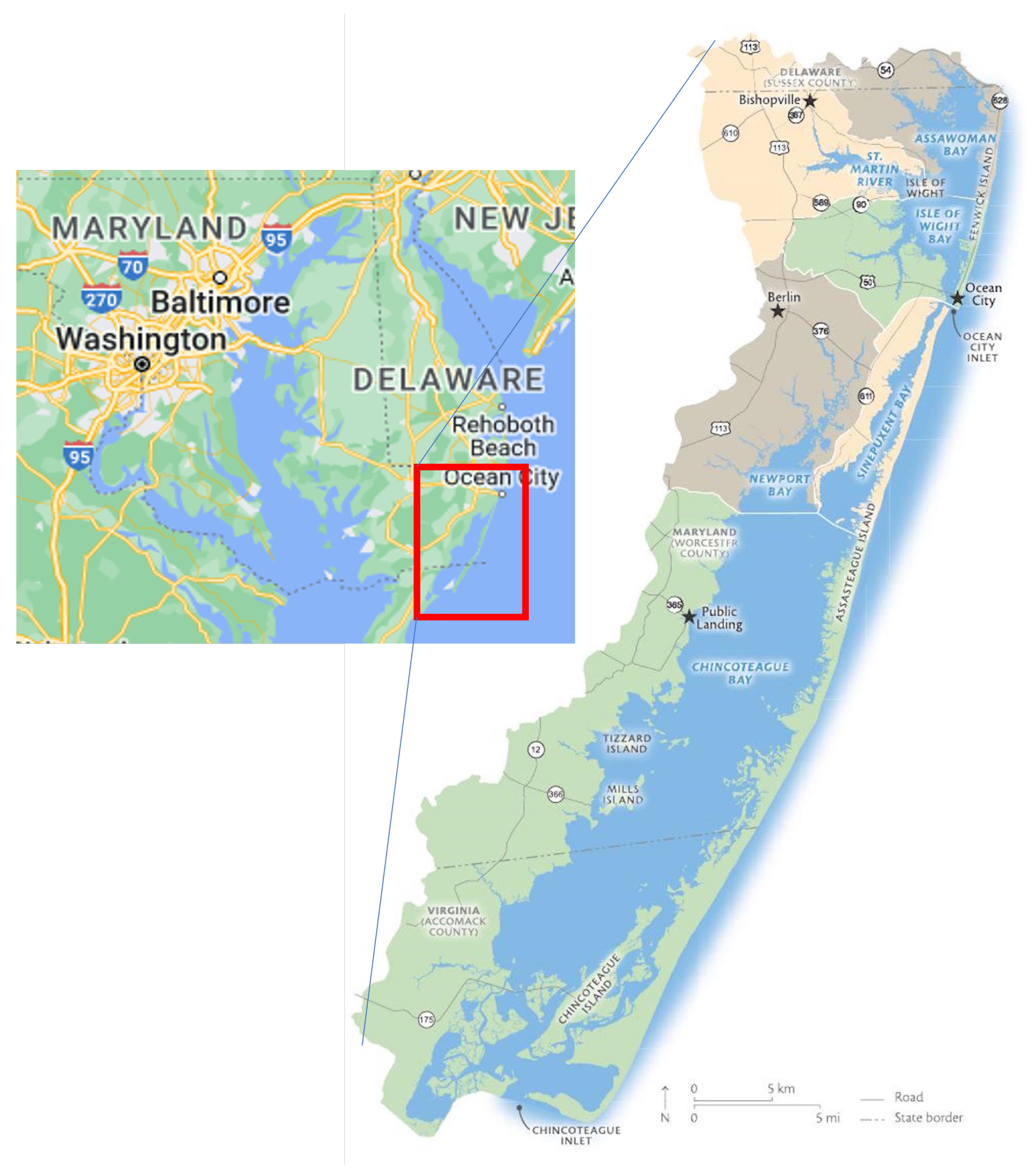
1.4. Chesapeake Bay Program
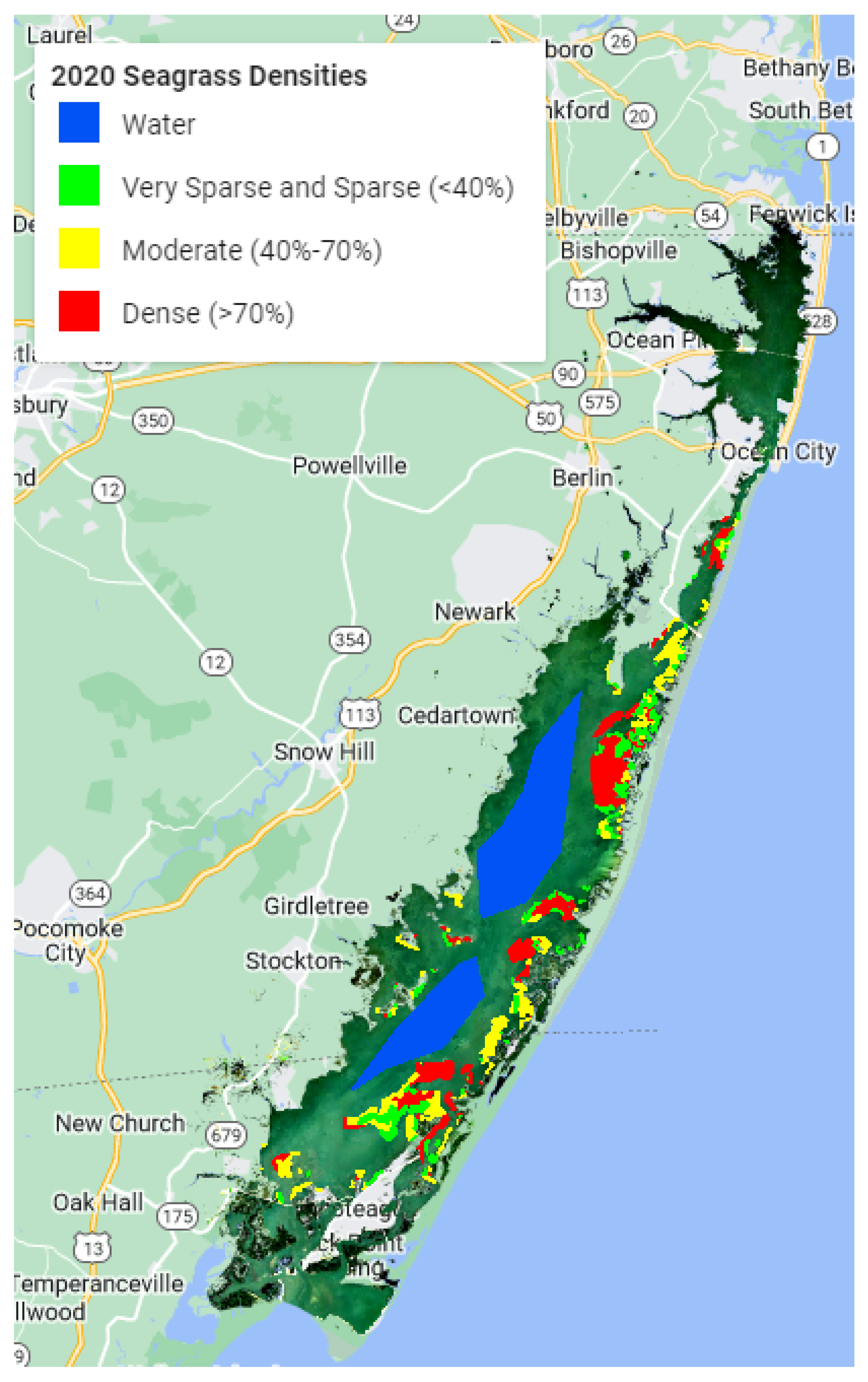
Seagrass has been closely monitored in the Chesapeake Bay since 1970 using RGB and NIR aerial imagery and ground samples, which is extremely expensive and time-consuming. Each year, multispectral (RGB and NIR) aerial imagery at 24 cm spatial resolution is collected. Concurrent ground surveys are conducted to confirm the existence of, and provide species data for, the seagrass beds. These efforts are very expensive and unfeasible for use in larger regions [
45]. These techniques are localized in order to be utilized on a larger scale. The goal of this study was to see if freely available medium-resolution Sentinel-2 data in Google Earth Engine (GEE) could be used with machine learning models to map seagrass density in the Chesapeake Bay region in order to assess machine learning model accuracy.
4. Discussion
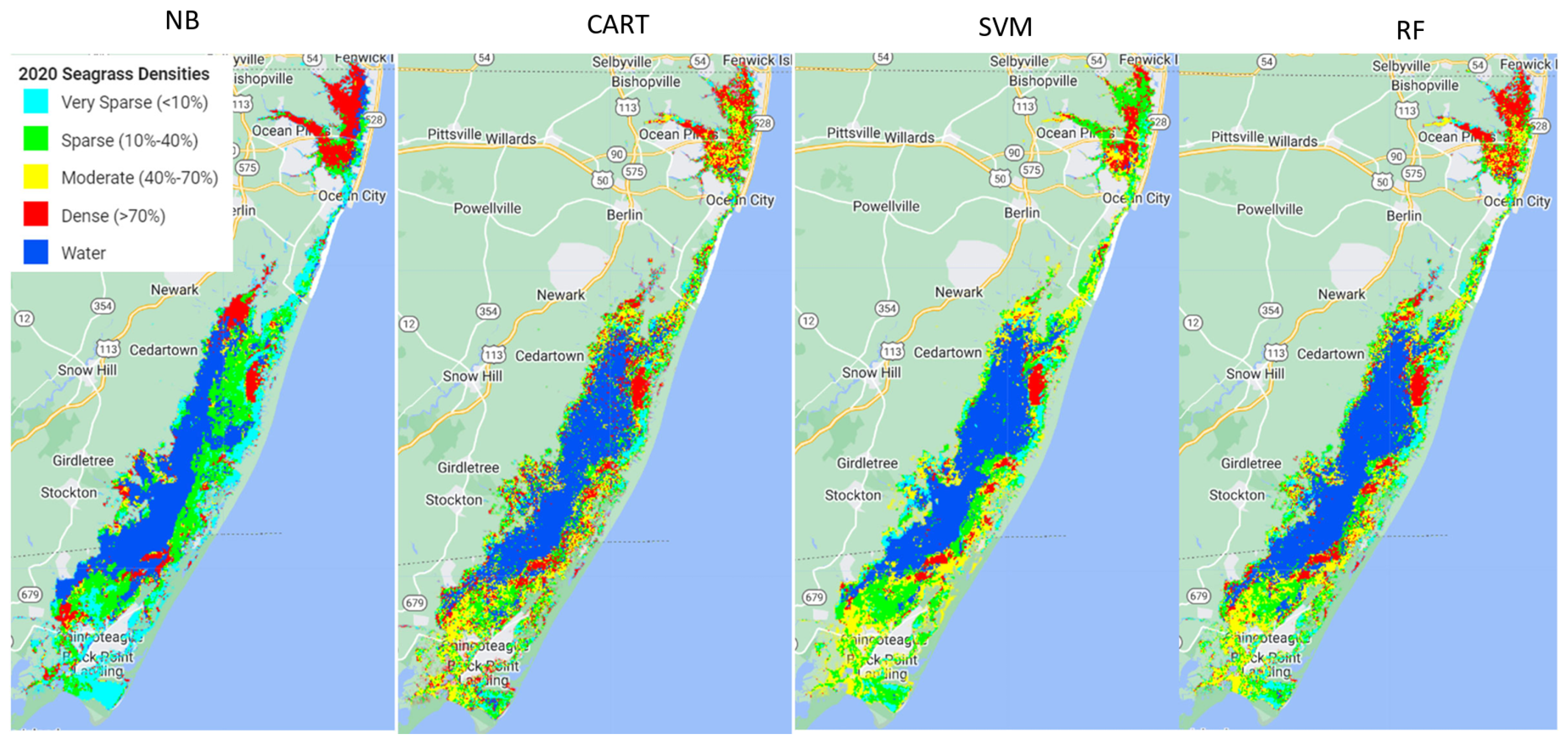
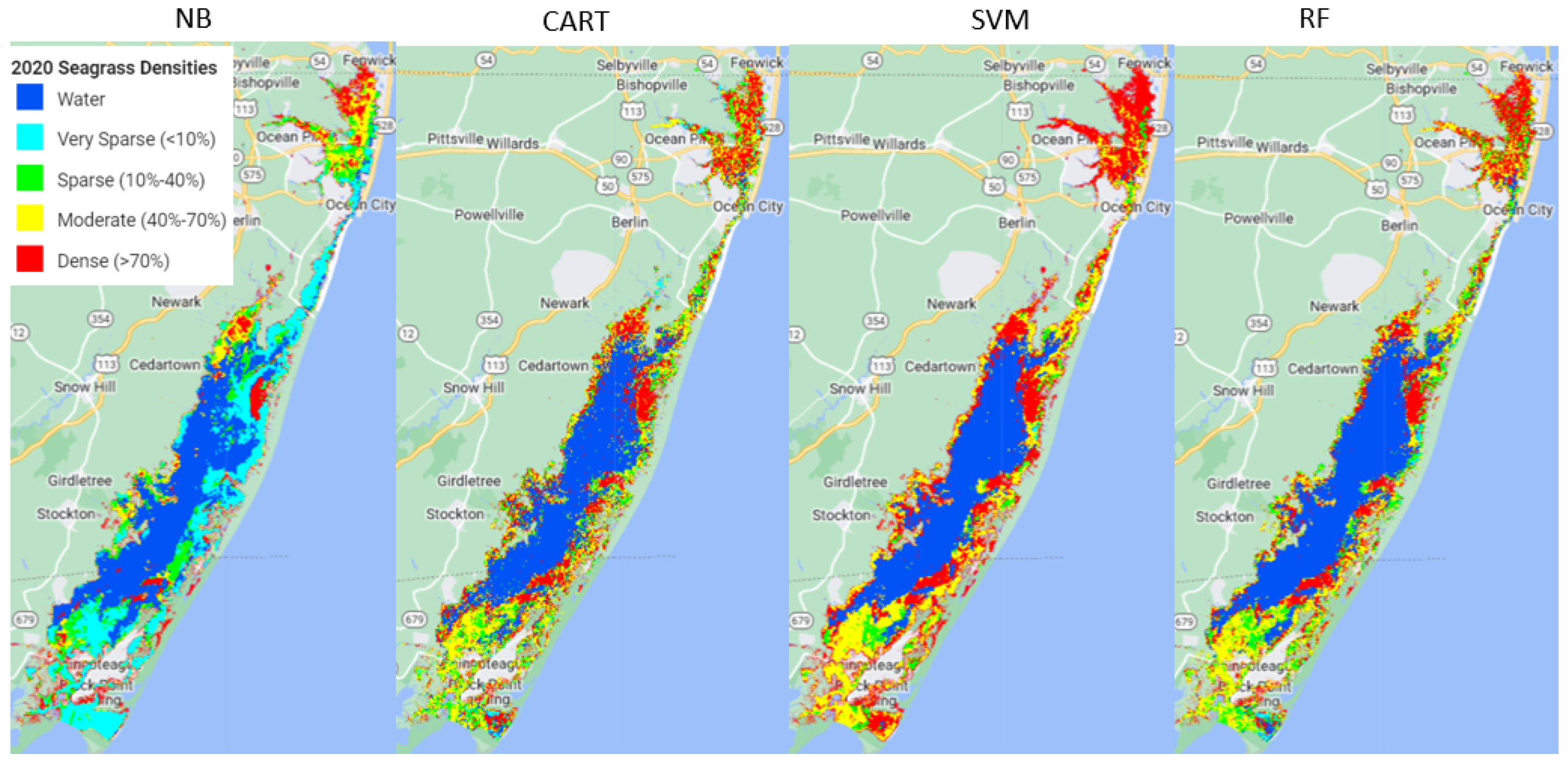
Out of the four machine learning algorithms (Naive Bayes (NB), Classification and Regression Trees (CART), Support Vector Machine (SVM), and Random Forest (RF)) tested in this study, RF outperformed the other three models, SVM and CART had very similar performance, and NB performed the poorest.
Using the available ground samples, both SVM and RF produced better consumer and producer accuracies for dense and moderate seagrass classes than for sparse and very sparse seagrass classes. The better performance for dense seagrass classes was reported in previous studies. For example, a study using hyperspectral imagery to map seagrass, also with a decision tree approach, found better performance at high densities of seagrass meadows [
32]. Another study used Maxar’s WorldView-2 and WorldView-3 high-spatial resolution commercial satellite to map with a deep convolution neural network (DCNN) and also found that satellite classification performed best in areas of dense, continuous seagrass compared to areas of sparse, discontinuous seagrass [
53]. A similar study used hyperspectral data and a maximum likelihood classification method to map seagrass density and achieved higher consumer accuracy for denser seagrass than sparser seagrass meadows and the producer accuracy was less dependent on the seagrass density [
33]. This finding is in agreement with our accuracy result using the SVM classifier. The conclusion seems logical. Satellite measurements cannot capture the fine spatial patterns in the distribution of plants and biomass within seagrass meadows, particularly in sparsely vegetated areas, due to its mixing with water column scattering [
33].
The analysis showed that model performance for each class depends on the training data size used. More training data available for denser seagrass classes may cause better model accuracy for dense seagrass classes. Previous studies have shown that training set size can greatly impact classification accuracy and consequently has been a major focus of attention in research [
54]. This research has generally found a positive relationship between classification accuracy and the size of the training set, following a power function for a wide range of classifiers [
55].
Further analysis of using a different training approach showed that when strategically using the same amount of ground samples for each class to train the models, the model accuracies were unrelated to seagrass density classes. This was evident using both the SVM and RF models (
Table 14 and
Table 15). The very sparse seagrass class tended to have the highest accuracy, followed by the dense seagrass class. The medium seagrass density classes had the lowest accuracy. Consumer accuracy, producer accuracy, and F1-score all showed consistent patterns using both the SVM and RF models. Our analysis demonstrates that the training data and how they can be properly trained can impact the model performance dramatically. We should be careful to implement the machine learning models properly.
Using the same sample size for each class for training and testing has some tradeoffs. It will reduce the overall accuracy. For example, when comparing two training methods (using all the ground samples and the equal sample size for each class), the overall accuracy decreased for RF from 0.874 to 0.818 and the Kappa coefficient from 0.777 to 0.774. This result suggests that there is a tradeoff when using all the ground samples versus using an equal number of ground samples for each class to train the model. More training data can result in more accurate overall model performance. Collecting a large training data set for supervised classifiers can be challenging, especially for studies covering a large area, which may be typical of many real-world applied projects [
56]. More innovative ideas, such as bootstrapping or Monte Carlo simulations, may help.
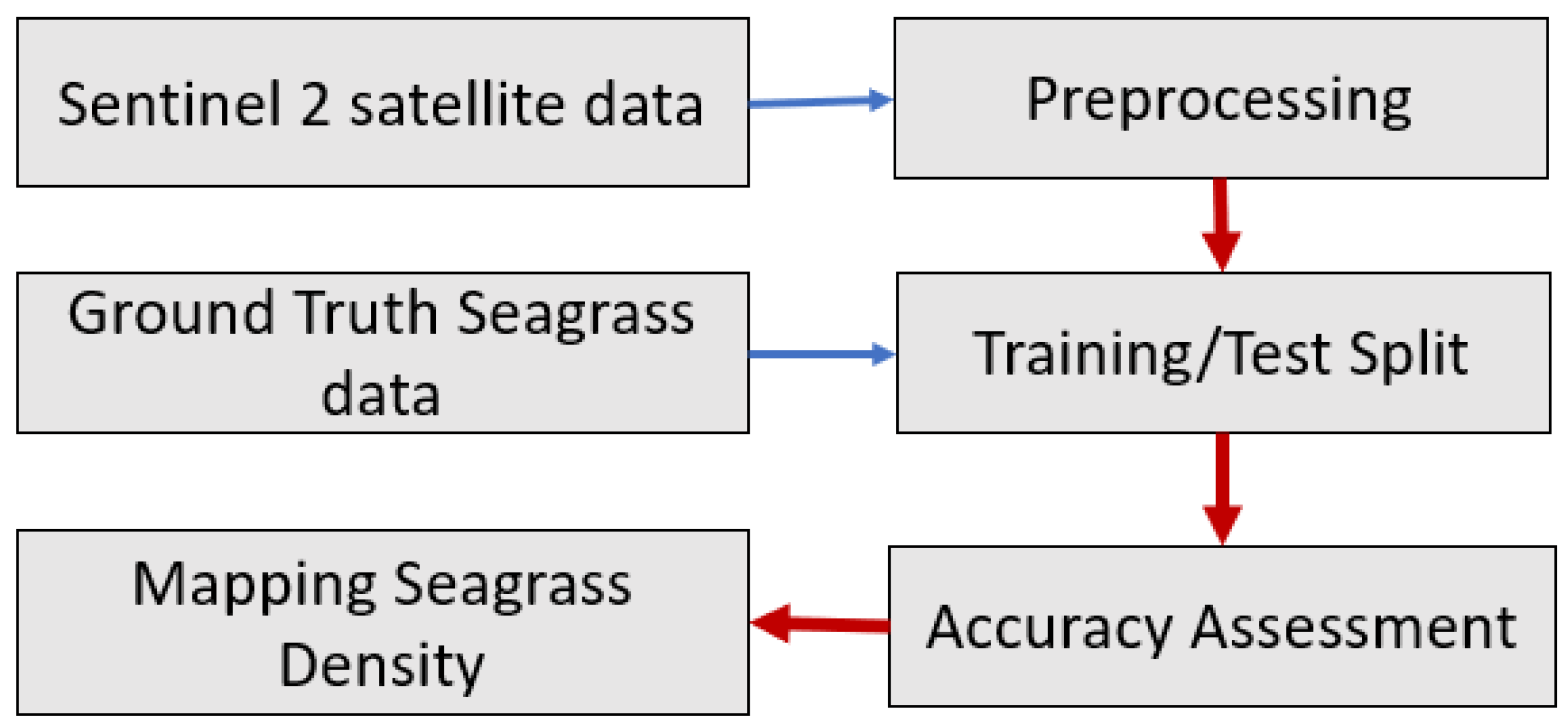
Many parts of the preprocessing could have been improved upon: In the pre-processing procedure of generating a clear composite image, we used the median value. A previous study showed that the first quartile yields less noisy image composites because it filters higher reflectances (clouds and sunlight) [
25]. Implementing the first quartile to generate a clear composite image might also improve the model’s performance.
Incorporating bathymetry data could improve the accuracy and make the model more transferable. The scattering and absorption in the water column impose an additional interference on the remotely sensed measurement of submerged habitats. The bathymetric dataset was used to correct light attenuation by the water column for resolving bottom reflectance [
26,
32]. The bathymetric data can be obtained from lidar and multispectral remote sensing data [
57]. Adding bathymetry data for this region could improve the model performance. However, a few studies found that water column correction had little improvement on mapping seagrass density, particularly when using machine learning classifiers on atmospherically corrected surface reflectance measurements [
31,
40]. The study in [
40] found that water column correction models only provide minor improvements in calm, clear, and shallow waters. Since the assumption of the water column correction model is invalid in complex and deep areas, water column corrections are discouraged in more complex scenarios with challenging water depths (25 and 35 m). However the study in [
31] argued that both models (random forests) are data-driven. Their finding should be restricted to single image analyses based on optimal water conditions (calm surface, lowest turbidity). The accuracy is an indicator of how well the model can fit the data. Similar accuracies do not indicate similar model transferability. However, they hypothesized that the water column corrected data might be better suited to transfer a random forest model to other image acquisitions.
The water body may have organic material other than seagrass, such as macroalgae and macrophytes, which use chlorophyll for photosynthesis [
58,
59]. Many studies classified seagrass and microalgae as separate classes [
3,
32,
60]. This study does not differentiate seagrass and other non-seagrass plant-like algae due to a lack of ground macroalgae data for training. Thus, the accuracy of identifying seagrass in this study could be overestimated if algae other than seagrass exist in Chesapeake Bay. Future work includes collecting ground macroalgae data and training the classifiers using ground samples of both seagrass and macroalgae.
5. Conclusions
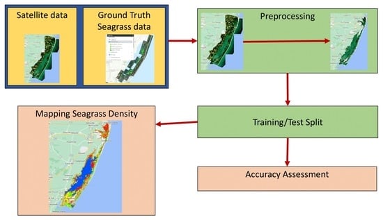
This study introduced a proof-of-concept procedure to map seagrass density in the Chesapeake Bay region using freely available medium-high spatial resolution (10 m, 20 m, and 60 m) Sentinel-2 data through machine learning models on Google Earth Engine, a flexible, time- and cost-efficient cloud-based system. Out of the four machine learning algorithms (Naive Bayes (NB), Classification and Regression Trees (CART), Support Vector Machine (SVM), and Random Forest (RF)) tested in this study, RF outperformed the other three models with overall accuracies of 0.874 and Kappa coefficients of 0.777. CART and SVM were very similar, and NB performed the worst. We tested two different approaches to assess the model’s accuracy. When using all the available training data, our analysis suggested the model performance was associated with seagrass density classes, wherein the denser the seagrass class, the better the models perform. However, when using the same size of training data for each class, the association of model performance with seagrass density classes disappeared. This analysis implies a false relationship of accuracies with seagrass density classes using all available ground samples to train and test the models. This finding suggested that one important factor determining overall accuracy is the training data and how to properly train the models in addition to the models selected. This study demonstrates the potential to map seagrass density using satellite data. For future work, instead of randomly splitting for training and testing, a new approach is required to remove the spatial-autocorrelation of satellite pixels to obtain the true accuracy of the machine learning models.


