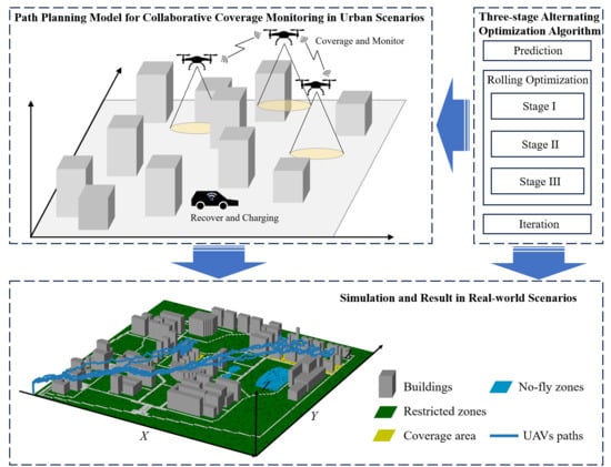
A Path Planning Method for Collaborative Coverage Monitoring in Urban Scenarios

Abstract

In recent years, unmanned aerial vehicles (UAVs) have become a popular and cost-effective technology in urban scenarios, encompassing applications such as material transportation, aerial photography, remote sensing, and disaster relief. However, the execution of prolonged tasks poses a heightened challenge owing to the constrained endurance of UAVs. This paper proposes a model to accurately represent urban scenarios and an unmanned system. Restricted zones, no-fly zones, and building obstructions to the detection range are introduced to make sure the model is realistic enough. We also introduced an unmanned ground vehicle (UGV) into the model to solve the endurance of the UAVs in this long-time task scenario. The UGV and UAVs constituted a heterogeneous unmanned system to collaboratively solve the path-planning problem in the model. Building upon this model, this paper designs a Three-stage Alternating Optimization Algorithm (TAOA), involving two crucial steps of prediction and rolling optimization. A three-stage scheme is introduced to rolling optimization to effectively address the complex optimization process for the unmanned system. Finally, the TAOA was experimentally validated in both synthetic scenarios and scenarios modeled based on a real-world location to demonstrate their reliability. The experiments conducted in the synthetic scenarios aimed to assess the algorithm under hypothetical conditions, while the experiments in the scenarios based on real-world locations provided a practical evaluation of the proposed methods in more complex and authentic environments. The consistent performance observed across these experiments underscores the robustness and effectiveness of the proposed approaches, supporting their potential applicability in various real-world scenarios.

1. Introduction

In recent years, path planning based on unmanned aerial vehicles (UAVs) has been one of the important issues in public security, intelligent transportation, and other application scenarios. This research topic has attracted the attention of many researchers. However, due to the limitations of vision, endurance, task load, and other aspects, a single UAV does not have the ability to deal with endurance and emergencies when performing complex and long-term tasks. In contrast, the collaborative use of multiple UAVs or even heterogeneous unmanned systems can improve the adaptability of task execution, which is also the main research content of path planning [1]. Moreover, within the context of constructing smart cities based on the Internet of Things (IoT), UAVs can be utilized for collecting localized sensor data within urban areas [2,3]. Utilizing UAVs for tasks in urban environments has proven to be an effective method. Leveraging the advantages of rapid response and agile maneuverability, UAVs have the capability to swiftly reach incident locations, offering real-time perspectives and valuable data support. This not only facilitates a prompt understanding of traffic conditions and accident scenes, but also furnishes crucial information for emergency rescue, traffic management, and task monitoring. The application of UAVs enhances the efficiency of information collection in emergency scenarios and eases ground traffic pressure, presenting new possibilities for urban traffic management. To achieve this, it is imperative to ensure the safe and timely arrival of UAVs at the designated target areas, thereby giving rise to the issue of UAVs’ path planning.

Aiming at this issue, many researchers have applied machine learning and neural networks to solve the problem of multi-UAV path planning, thereby improving the timeliness and robustness [4,5]. Papaioannou et al. [6] introduced Reinforcement Learning (RL) to plan the integrated ray-tracing and coverage control of UAVs, which addressed the problem of autonomous UAV coverage by formulating it as a Markov Decision Process (MDP). Theile et al. [7] leveraged an improved RL approach to learn a control policy for UAVs that generalizes over random start positions and varying power constraints and decides between multiple landing positions, which successfully balances the safe landing and coverage of the target area. Tolstaya et al. [8] trained a graph neural network controller that leverages the spatial equivariance of the task to imitate an expert open-loop routing solution, which effectively generated a feasible plan for multi-robot coverage and exploration tasks.

Mixed-Integer Programming (MIP) is also a popular method in this field. Papaioannou et al. [9] proposed a receding horizon coverage control approach for multiple autonomous aerial agents to cooperatively cover the total surface area of a 3D object of interest. They demonstrated the transformation of non-linear and non-convex visibility determination constraints into logical constraints embedded within a mixed-integer optimization problem. Choi et al. [10] converted the Coverage Path Planning (CPP) problem into a Mixed-Integer Linear Programming (MILP) problem with energy constraints and presented a new CPP method for an aerial imaging mission with multiple UAVs by introducing a new route-based optimization model with column generation. Papaioannou et al. [11] presented a novel distributed search-planning framework for cooperative 3D object search by dynamically varying autonomous agents. It leveraged Model Predictive Control (MPC) and utilized a Mixed-Integer Quadratic Programming (MIQP) formulation, demonstrating an efficient solution with widely available optimization tools. Aiming at the CPP problem of autonomous heterogeneous UAVs on a bounded number of regions, Chen et al. [12] proposed an exact formulation based on MILP and a original clustering-based algorithm to classify regions into clusters and obtain approximate optimal point-to-point paths for UAVs such that coverage tasks would be carried out correctly and efficiently. Papaioannou et al. [13] proposed an integrated guidance and gimbal control CPP approach and jointly controlled and optimized the UAV mobility and gimbal inputs, which is solved by using MIQP. The proposed approach was demonstrated to effectively achieve full coverage of a given region of interest.

As a new and popular method to deal with optimization problems, the swarm intelligence-optimization method has also been the focus of swarm path planning recently. Misra et al. [14] proposed an NP-hard multi-objective optimization problem of maximizing surveillance area coverage using multiple UAVs in an obstacle-laden and Global Positioning System (GPS)-denied environment and solved it by using a modified Particle Swarm Optimization (PSO) implemented on a multi-core CPU for faster convergence without violating the feasibility criteria. Zhang et al. [15] devised a novel approach to solve the problem of generating optimal flight paths for UAVs across a three-dimensional environment. Their method reformulated the problem as a constrained optimization problem and utilized an enhanced constrained Differential Evolution (DE) algorithm to achieve stable cooperative flight among multiple UAVs. Zhen et al. [16] introduced an innovative cooperative mission-planning strategy for UAV swarms to enhance the overall search capability of UAVs. This approach aimed to efficiently locate and engage time-sensitive moving targets in dynamic and uncertain environments through a Hybrid Artificial Potential Field and Ant Colony Optimization (HAPF-ACO) algorithm. Aiming at the NP-hard computational complexity of CPP for UAVs in large-scale cooperative search systems, Chen et al. [17] proposed an Ant Colony System (ACS)-based algorithm to obtain good enough paths for UAVs and fully cover all regions efficiently.

In handling the problem of UAV or multi-UAV path planning, machine learning, MIP, and the swarm intelligence-optimization algorithm are commonly employed methods. Machine learning learns the optimal strategy through the interaction between agents and the environment, suitable for dynamic environments in path-planning problems, but it faces the challenges of high computational complexity in large-scale problems [18,19,20]. MIP transforms the path-planning problem into a mathematical model and solves it to obtain the optimal solution, suitable for static environments in path planning, but struggles to cope with complex dynamic environments [21,22]. Swarm intelligence-optimization algorithms, such as the Sparrow Search Algorithm (SSA), Genetic Algorithm (GA), and PSO, simulate collective cooperation behavior to find optimal solutions in large-scale, dynamic, and complex environments. These algorithms possess a good global search capability and robustness [23,24]. Additionally, swarm intelligence-optimization algorithms typically have lower computational complexity, enabling them to find near-optimal solutions in a shorter time, demonstrating high practicality and efficiency. On this basis, considering the complexity of the multi-UAV cooperative path-planning model and the diversity of environmental constraints, this paper uses a swarm intelligence-optimization algorithm to solve the cooperative model.

However, it is a challenging task for UAVs to conduct efficient path planning consistently. The objective is to find the optimal path from the starting point to the destination, considering factors such as path length, safety, and smoothness [25]. The key research focus is on coordinating UAV swarms and ensuring autonomous endurance during mission execution in three-dimensional complex urban environments. Existing studies frequently utilize systems composed of a single UAV, a UAV swarm, or unmanned systems composed of UAVs and UGVs to autonomously complete path-planning tasks. The coordination between UAVs and UGVs is a forward-looking research topic with wide-ranging practical applications. Moreover, UGVs can serve as charging stations for UAVs [26], ensuring a certain level of endurance for UAVs during the path-planning process. Therefore, this paper focuses on a UAV and UGV system for path-planning problems in three-dimensional complex urban environments, aiming at minimizing task completion time.

The application of unmanned system collaborative tasks is a current topic of great interest for researchers. In Reference [27], a UAV and UGV system was utilized for precise joint localization of ground targets. Minaeian et al. [28] employed a UAV and UGV system to identify and track target individuals in border areas. The system used a UAV for coarse detection with low resolution and wide coverage and integrated the high-resolution and high-fidelity detection capabilities of UGVs to accurately locate detected individuals with unknown independent movement patterns. Ghamry et al. [29] applied a UAV and UGV system to the scenario of forest fire detection. Utilizing the extensive aerial sensing capabilities of UAVs and the robust on-board computing power and payload capacity of UGVs, collaborative efforts were made to search for and continuously monitor forest fires.

Qin et al. [30] employed a UAV and UGV system to autonomously explore, map, and navigate in three-dimensional unknown environments where GPS information is not available. Through the collaborative efforts of UGVs for coarse detection and UAVs for detailed mapping, complementary mapping results were shared to generate an optimal exploration path. Lakas et al. [31] focused on path planning in unknown environments affected by natural disasters or warfare using a UAV and UGV system, in which the UAV gathered ground building information to guide real-time path planning for the ground UGVs. Asadi et al. [32] utilized a UAV and UGV system to implement a high-frequency and highly autonomous data-collection scheme. The UAV detected blind spots inaccessible to the UGVs, obtaining global information to assist the UGVs in obstacle avoidance and low-energy path planning. Wei et al. [33] focused on path planning in general outdoor and indoor environments where GPS cannot provide normal localization. The UAV provided aerial visibility to the UGVs, while the UGVs considered obstacle avoidance and optimized energy consumption during path planning. Both studies [32,33] involved UAVs providing auxiliary visibility for UGVs in path planning. In contrast, this paper specifically investigates how UGVs assist in enhancing the endurance of UAVs during path planning. Li et al. [34] utilized a UAV to capture ground images from aerial vision, constructing ground maps to aid the UGV in accurately identifying obstacles for path-planning tasks. However, all UGV path points were derived from obstacle vertices, making the path essentially not globally optimal, especially considering the small allowable error in real-world scenarios.

In summary, inspired by References [24,35], this paper proposes an unmanned system path-planning method in an urban environment and conducts modeling and experiments as close as possible to the reality. The main contributions of this paper are as follows:

• Due to their limited endurance capability, UAVs alone are not well suited for long-term tasks. To address this limitation, this paper introduces UGVs into the model, leveraging their additional power capacity to enhance the endurance of the UAVs. By incorporating UGVs, the model forms a heterogeneous unmanned system that collaboratively tackles the path-planning problem.
• Conventional optimization methods struggle to effectively optimize problems involving complex interactions among multiple and heterogeneous agents. To tackle this challenge, we propose a Three-stage Alternating Optimization Algorithm (TAOA) to iteratively optimize the unmanned path-planning problem. This algorithm ensures both the effectiveness and efficiency of the solution.
• We integrated the design of restricted zones and no-fly zones into the environmental model, thereby enhancing the authenticity and efficacy of the model. For the experiments, we constructed a simulated environment mapped based on a real-world region. Through simulation experiments conducted in both synthetic and real-world scenarios, the proposed path-planning model and optimization method demonstrated enhanced credibility.

The rest of this paper is structured as follows. Section 2 describes the proposed model, including the urban environment, unmanned system, and objective function. Section 3 presents the proposed method, and the simulation results alongside useful discussions are provided in Section 4. Finally, the conclusion of this work is given in Section 6.

2. Model

In this model, UAVs are primarily tasked with flying from the takeoff point to the starting point of the coverage search task, performing the coverage search task, and ultimately, returning. This proposed model is based on existing city region maps, indicating that the unmanned system possesses prior knowledge of global information. The task region is divided into numerous equidistant cubes [24], with their respective centers serving as plausible waypoints for UAV flight trajectories. Consequently, the two-dimensional plane encompassing the terrestrial component of the task region is segmented into uniform two-dimensional grids. The centers of these grids are considered potential waypoints for UGV paths. Building upon this task region modeling, this section further elaborates on the model details.

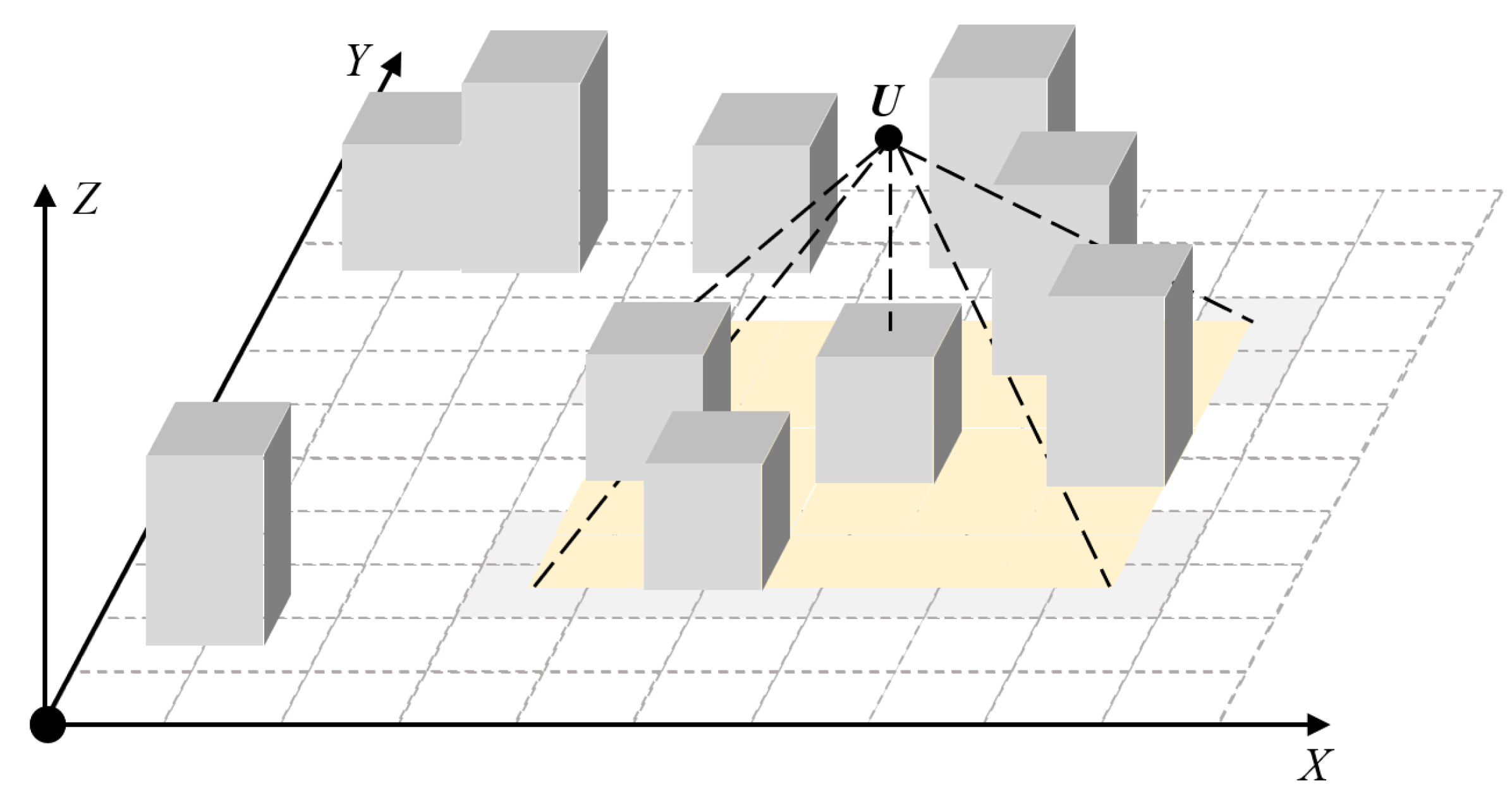
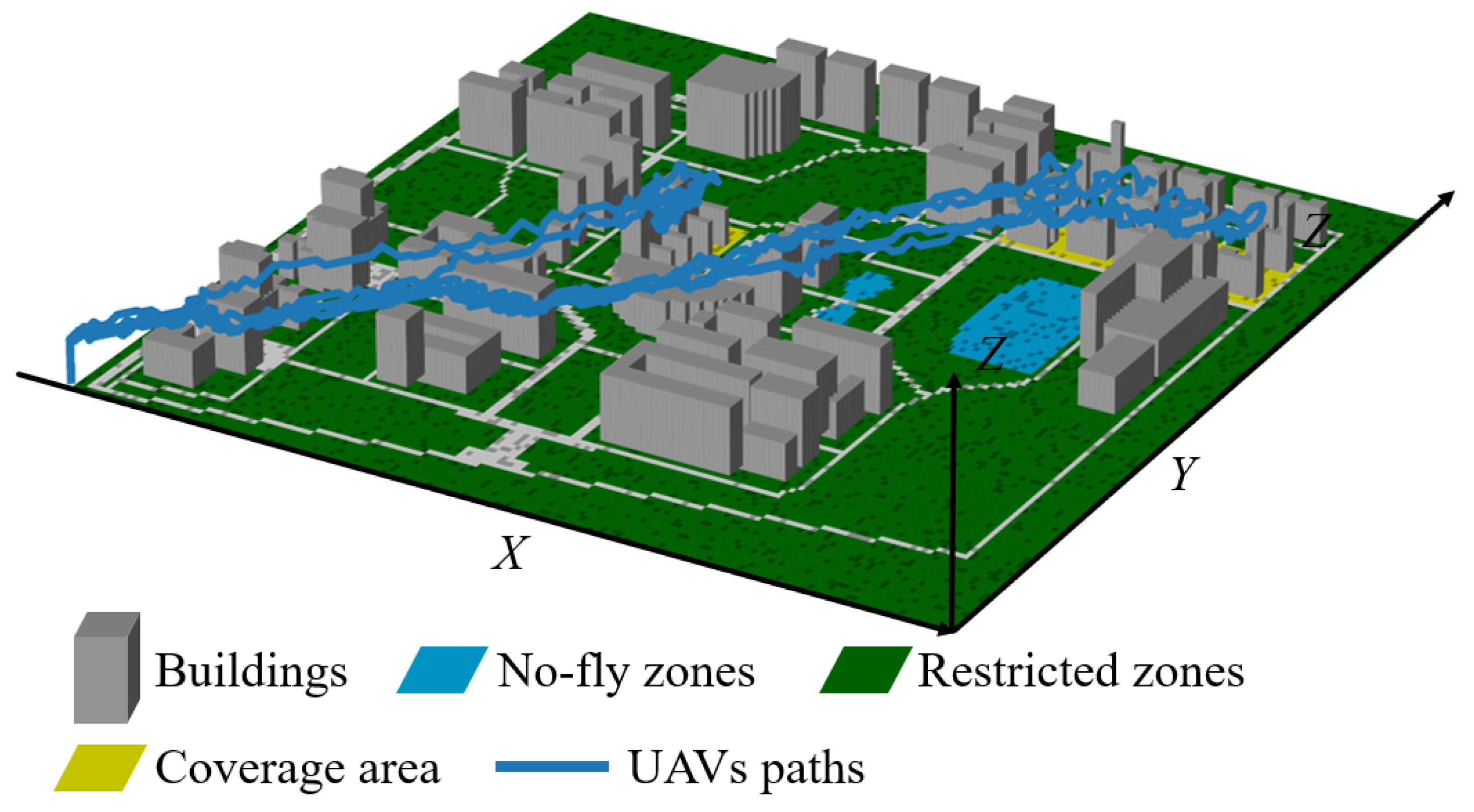
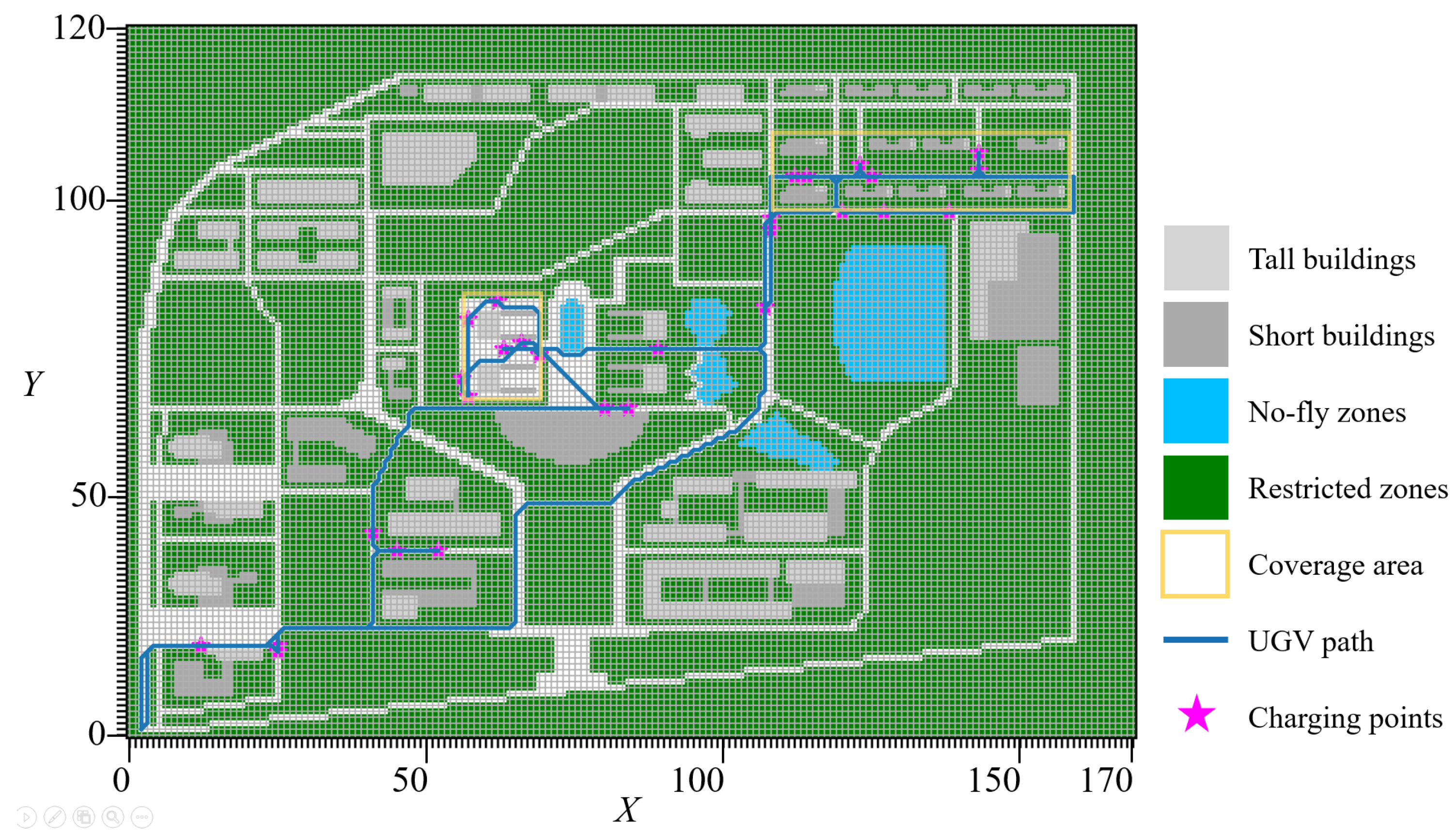
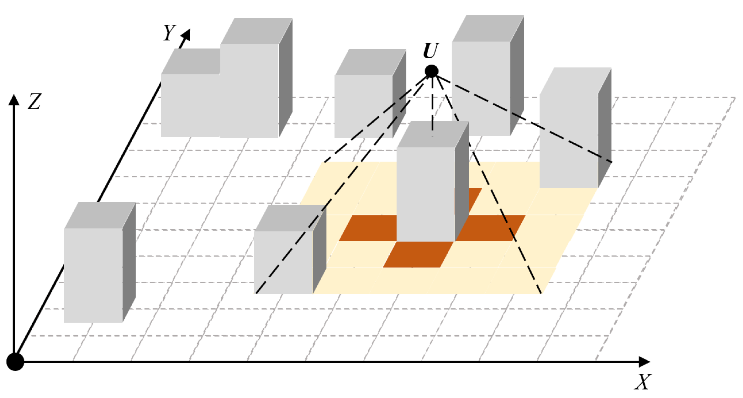
2.1. Environment Model and Problem Description

In this paper, the urban scenario is modeled as a three-dimensional coordinate system, and the coordinates of any point in the space are $(m,p,q)$, while its index is k, where $m\in \{1,\dots ,X\},p\in \{1,\dots ,Y\},q\in \{1,\dots ,Z\}$. The whole space is divided into $X\times Y\times Z$ cubes, and the total size is $L_x\times L_y\times L_z$. Therefore, a Digital Elevation Model (DEM) D for the urban scenario is given by $D=\left\{(x_m,y_p,z_q)\right\}$. In the urban scenario, buildings are distributed on the ground in the lower airspace. This paper uses cubes in D to represent buildings. Two different heights, $h_1$ and $h_2$$(Z>h_1>h_2)$, were set to simulate uneven building heights in the city. Additionally, to simulate real-world scenarios, this paper introduces no-fly zones and restricted zones into the environment model to respectively constrain the movement of the UAVs and UGV. A schematic diagram of the simulated scenario is illustrated in the Figure 1.

The path-planning task is undertaken by the UAVs, executing the coverage search missions in their designated coverage areas. The UGV plans its path based on the routes of the UAVs. When one UAV’s energy drops below a certain level during the task, the UGV is mobilized to charge the UAV. The objective is to enable the UAVs to complete the coverage mission in the shortest possible time. The model is subject to the following assumptions:

• The UAVs are prohibited from flying above any height in no-fly zones, and the UGV is not allowed to traverse restricted zones.
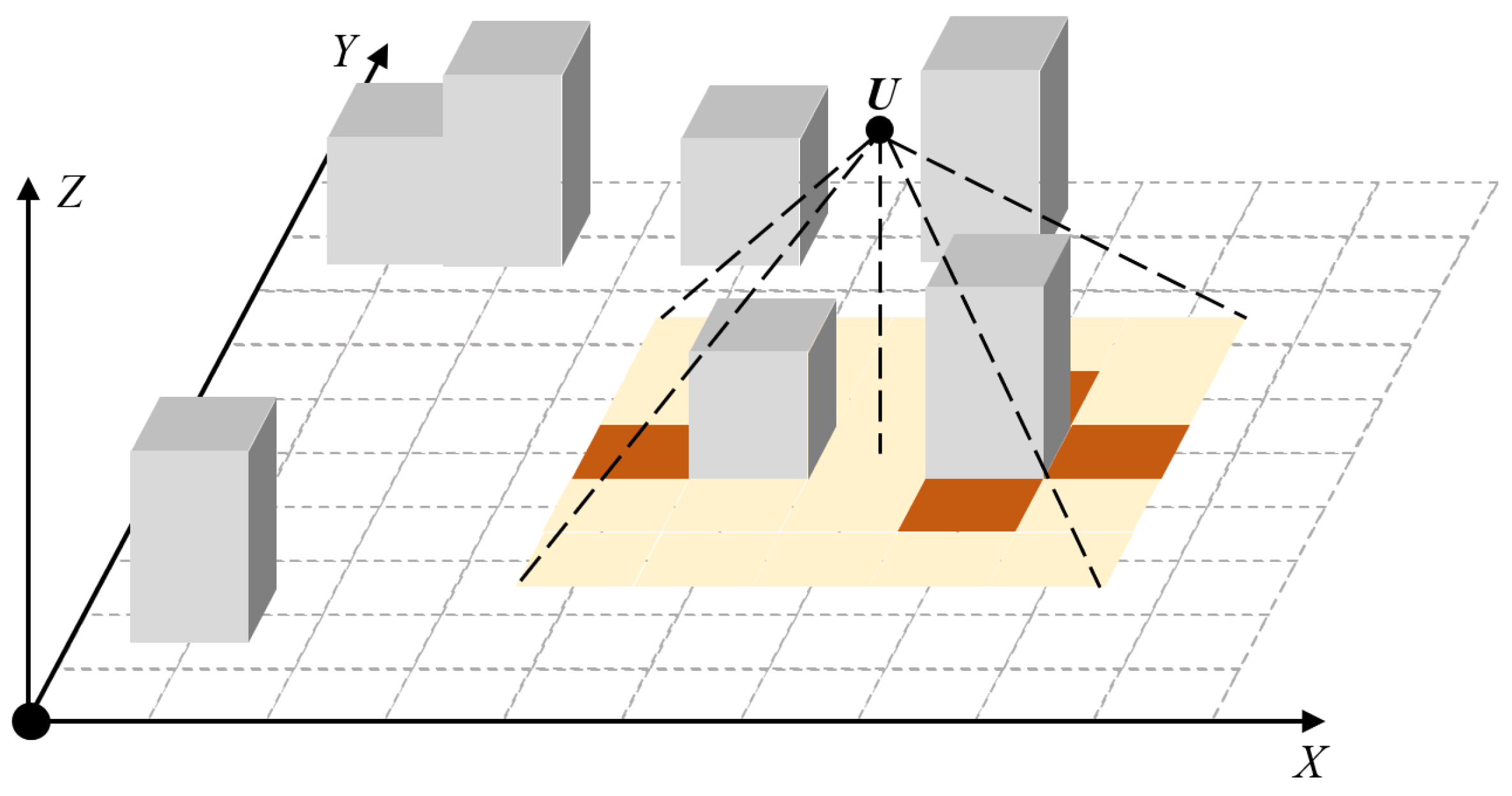
• The coverage search task for the UAVs has specific requirements for the image resolution, meaning the UAVs must descend to the specified flight altitude to achieve effective coverage.
• The UAVs and UGV have a constraint on the total energy.
• The UAVs need to reserve some battery capacity for hovering and waiting for the UGV to arrive for recharging.
• Only the UAVs hovering above the UGV can be reclaimed and recharged by the UGV.

2.2. Unmanned System Model

2.2.1. Motion Model

The set of UAVs is denoted as $UAV=\{U_1,U_2,\dots ,U_{N_A}\}$, where $N_A$ is the total number of UAVs. As shown in Figure 2, a UAV located at the center of a cube can choose the center of any of the external $3\times 3\times 3$ cubes as the next path point. At each moment, the UAV has 27 movable directions, including the option to hover in its original position. The original location of the UAV is represented by a black dot, and the path points that can be selected are represented by a red dot in Figure 2. In the horizontal direction, the UAV cannot move outside the task area. In the vertical direction, the UAV cannot descend below the minimum takeoff height $h_{min}^{uav}$ or ascend above the maximum flying height $h_{max}^{uav}$ during the task. Additionally, UAVs are prohibited from flying above no-fly zones $R_a$, and the UGV is prohibited from traversing restricted zones $R_u$. At time t, the UAV $U_i$ has a motion velocity vector $V^{uav,i}\left(t\right)$ and the energy consumption per time-step of the UAV only in flight is $E^{uav,i}\left(t\right)$.

As shown in Figure 3, the UGV is denoted as G. A UGV located at the center of a two-dimensional grid can choose any of the centers of the surrounding $3\times 3$ grids as the next movement point, meaning that UGV has 9 movable directions, including the option to remain stationary. The original location of the UGV is represented by a black dot, and the path points that can be selected are represented by a red dot in Figure 3. The UGV cannot move outside the task area, and it is prohibited from driving into restricted zones. At time t, the UGV has a motion velocity vector $V^{ugv}\left(t\right)$, and the energy consumption per time-step of the UGV in motion is $E^{ugv}\left(t\right)$.

Inspired by [36], this paper divides the energy consumption of the UAV into three parts: path energy consumption, turning energy consumption, and climbing energy consumption; the equations are as follows.

$$E^{uav,i}\left(t\right)=E_{path}^{uav,i}\left(t\right)+E_{turn}^{uav,i}\left(t\right)+E_{climb}^{uav,i}\left(t\right)$$

(1)

$$E_{path}^{uav,i}\left(t\right)=q_1·{\alpha }_i\left(t\right)$$

(2)

$$E_{turn}^{uav,i}\left(t\right)=q_2·{\mu }_0·(1+cos{\beta }_i\left(t\right))$$

(3)

$$E_{climb}^{uav,i}\left(t\right)=q_3·\gamma \left(t\right),$$

(4)

where $q_1$, $q_2$, and $q_3$ are scale factors. ${\mu }_0$ denotes the turning angle coefficient of the UAV. ${\alpha }_i\left(t\right)$ denotes the Euclidean distance that the ith UAV travels in the horizontal direction at time t; ${\beta }_i\left(t\right)$ denotes the deflection angle of the ith UAV in the horizontal direction at time t; ${\gamma }_i\left(t\right)$ denotes the absolute value of the ith UAV’s motion in the vertical direction at time t.

Similarly, the energy consumption of the UGV in motion is expressed by the following equation.

$$E^{ugv}\left(t\right)={\mu }_1·(1+cos\delta \left(t\right)),$$

(5)

where ${\mu }_1$ denotes the turning angle coefficient of the UGV, and $\delta \left(t\right)$ denotes the deflection angle of the UGV at time t.

2.2.2. Endurance and Bearing Model

The complexity of urban environments tends to prolong the overall task duration, demanding high endurance requirements for UAVs. The model integrates a UGV to offer autonomous landing and recharging services for UAVs [37,38], thus ensuring mission autonomy. Regarding the autonomous charging aspect, there are currently relevant technologies available on the market. For instance, the DJI Matrice 300 RTK is equipped with a non-contact fast charging module, capable of charging the battery from 20% to 90% in approximately 32 min.

$E_{init}^{uav}$ and $E_{init}^{ugv}$ are the energy level of one UAV and the UGV, respectively, when they are fully charged. The charging mechanism is that the UGV consumes energy $E_{charge2}$ to charge the UAV energy of $E_{charge1}$ at each time-step $\Delta t$ and $E_{charge2}>E_{charge1}$. When the battery level of a particular UAV is not full, the UGV will decide whether to initiate charging and determine the amount of charge required.

Additionally, if at time t, the UAV is in flight and satisfies the fourth and fifth assumptions in Section 2.1, it can choose to descend to be recovered by the UGV, which takes energy $E_{descend}^{uav}$. Similarly, if the UAV is being transported by the UGV, the UAV can choose to take off, which takes energy $E_{takeoff}^{uav}$. The additional energy consumption for the UGV to carry one UAV is denoted as $E_{carry}^{ugv}$. The energy consumption for deploying and retrieving UAVs is represented by $E_{throw}^{ugv}$ and $E_{pick}^{ugv}$, respectively. The UGV has the capability to carry all UAVs, but at any given time, it can only charge up to $N_C$ UAVs, where $N_C<N_A$.

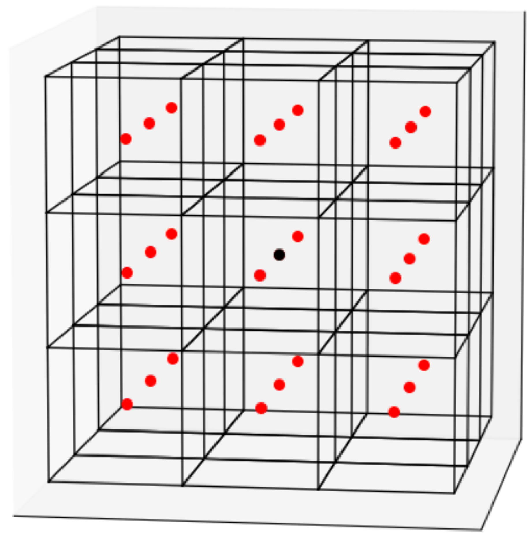
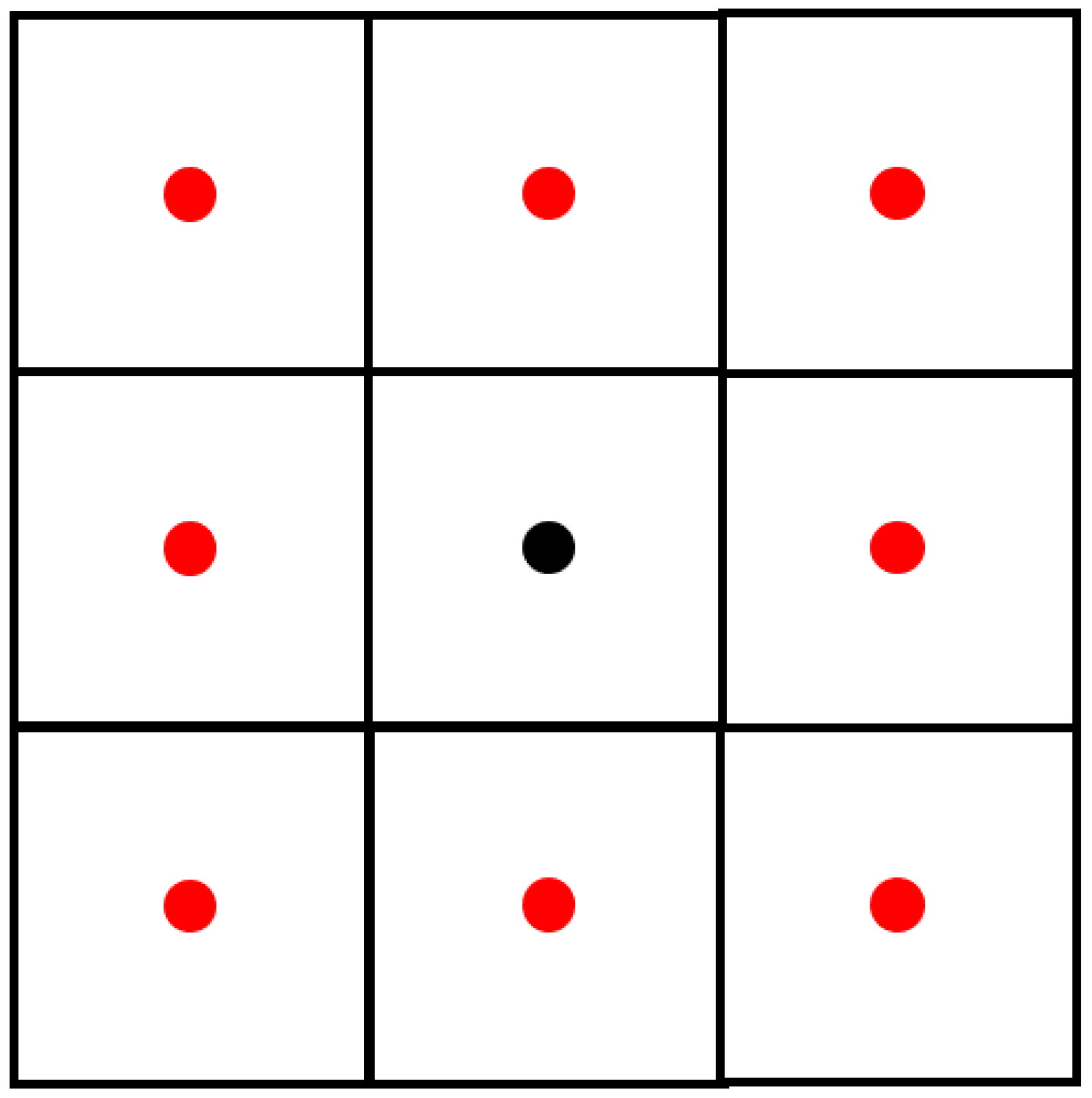
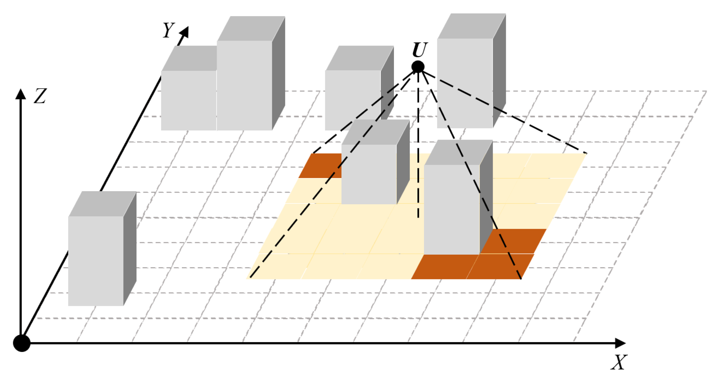
2.2.3. Sensor and Cognitive Map Model

Each UAV is installed with a sensor for the coverage search task, and the coverage area of ith UAV at time t is denoted as $C_i\left(t\right)$. Inspired by [39] and in conjunction with the design of the urban environment model, this paper set the coverage search area for a single UAV as illustrated by the yellow region in the Figure 4, Figure 5, Figure 6 and Figure 7, to better reflect the influence of building occlusion on the model and method in the experimental section. It is important to note that, in the second assumption of Section 2.1, we specified that effective coverage by the UAV must occur at a designated altitude. Therefore, the coverage range of the UAV is only affected by buildings within the designated coverage area. The different obstruction situations, represented by cases (a), (b), (c), and (d) in Figure 4, Figure 5, Figure 6 and Figure 7 respectively, are illustrated with buildings with different heights at different positions within the coverage of the UAV. Areas obscured by buildings that cannot be covered are indicated by the orange region. The UAV consumes additional energy $E_{cover}^{uav}$ per time-step during the coverage search task.

Each UAV keeps a cognitive map and holds information collected from sensors about the environment to help coverage and search. The cognitive map is constantly updated based on the detection results and information. This paper uses the map of target existence probability to describe the UAVs’ cognitive information. $p_{ik}\left(t\right)$ refers to the probability that the region needing detection exists in the kth grid at time t in the cognitive map of the ith UAV. The ith UAV considers that there is region needing detection when $p_{min}\le p_{ik}\left(t\right)\le p_{max}$, where $p_{min}$ and $p_{max}$ are constants satisfying $0<p_{min}<p_{max}<1$. The commonly used method of updating the probability map by the sensor observations $o_{ik}\left(t\right)$ is based on the Bayesian rule [40], which is given by Equation (6).

$$\begin{array}{cc}\hfill p_{ik}\left(t\right)& =\frac{p\left(o_{ik}\left(t\right)\right|{\theta }_k=1)p_{ik}(t-1)}{p\left(o_{ik}\left(t\right)\right|{\theta }_k=1)p_{ik}(t-1)+p\left(o_{ik}\left(t\right)\right|{\theta }_k=0)(1-p_{ik}(t-1))}\hfill \\ \hfill & =\left\{\begin{array}{c}\frac{p_d{p}_{ik}(t-1)}{p_d{p}_{ik}(t-1)+p_f(1-p_{ik}(t-1))},k\in C_i\left(t\right)\left(t\right),o_{ik}\left(t\right)=1,\hfill \\ \frac{(1-p_d)p_{ik}(t-1)}{(1-p_d)p_{ik}(t-1)+(1-p_f)(1-p_{ik}(t-1))},k\in C_i\left(t\right)\left(t\right),o_{ik}\left(t\right)=0,\hfill \\ p_{ik}(t-1),k\notin C_i\left(t\right)\left(t\right)\hfill \end{array}\right.\hfill \end{array}$$

(6)

where ${\theta }_k=1$ means that there is region needing detection in $C_i\left(t\right)$ of the ith UAV at time t, and ${\theta }_k=0$ means that there is no region needing detection in $C_i\left(t\right)$; $o_{ik}\left(t\right)=1$ indicates that the ith UAV detects the region needing detection in the kth grid, and $o_{ik}\left(t\right)=0$ indicates that the ith UAV detects no region needing detection in the kth grid. $p_d$ and $p_f$ are the detection probability and false alarm probability, respectively.

To reduce the computational complexity, the following nonlinear transformation of the probability map is introduced when $0<p_{ik}\left(0\right)<1$ [41].

$${\widehat{p}}_{ik}\left(t\right)\stackrel{\Delta }{=}ln(\frac{1}{p_{ik}\left(t\right)}-1).$$

(7)

Consequently, Equation (7) is transformed into a linear update as follows.

$${\widehat{p}}_{ik}\left(t\right)={\widehat{p}}_{ik}(t-1)+v_{ik}\left(t\right),$$

(8)

where

$$v_{ik}\left(t\right)\stackrel{\Delta }{=}\left\{\begin{array}{c}ln\frac{p_f}{p_d},k\in C_i\left(t\right),o_{ik}\left(t\right)=1,\hfill \\ ln\frac{1-p_f}{1-p_d},k\in C_i\left(t\right),o_{ik}\left(t\right)=0,\hfill \\ 0,k\notin C_i\left(t\right).\hfill \end{array}\right.$$

(9)

Thus, ${\widehat{p}}_{ik}\left(t\right)$ can help the UAVs simplify the calculations instead of $p_{ik}\left(t\right)$ [42]. The above derivation ensures that each UAV has a cognitive map to help it update the information of the environmental in real time.

2.3. Constraints

2.3.1. Obstacle Constraint

Ensuring the avoidance of collisions between UAVs and obstacles is a primary consideration in the seamless execution of tasks. This becomes particularly crucial in the urban environment, where the primary obstacles are tall buildings, introducing an extra layer of complexity to the collision-avoidance strategy. Effective obstacle avoidance ensures safety and reliability in the operation of UAVs within the urban environment. Therefore, based on the DEM in Equation (10) and the UAV model in Equations (11) and (12), the obstacle constraint for the UAVs is presented in Equation (15). Similarly, the UGV is represented in Equations (13) and (14), and the obstacle constraint for the UGV is presented in Equation (16).

$$\begin{array}{c}D=\left\{\right(m,p,q\left)\right\}\end{array}$$

(10)

$$\begin{array}{c}UAV=\{U_1,U_2,\dots ,U_{N_A}\}\end{array}$$

(11)

$$\begin{array}{c}{U}_i=\{(x_i^a\left(0\right),y_i^a\left(0\right),z_i^a\left(0\right)),(x_i^a\left(1\right),y_i^a\left(1\right),z_i^a\left(1\right)),\dots ,(x_i^a\left(T\right),y_i^a\left(T\right),z_i^a\left(T\right))\}\end{array}$$

(12)

$$\begin{array}{c}UGV=\left\{G\right\}\end{array}$$

(13)

$$\begin{array}{c}G=\{(x^g\left(0\right),y^g\left(0\right),z_1^g\left(0\right)),(x^g\left(1\right),y^g\left(1\right),z^g\left(1\right)),\dots ,(x^g\left(T\right),y^g\left(T\right),z^g\left(T\right))\}\end{array}$$

(14)

$$\begin{array}{c}{U}_i\cap D=\varnothing ,i=1,2,\dots ,N_A\end{array}$$

(15)

$$\begin{array}{c}G\cap D=\varnothing ,\end{array}$$

(16)

where $(m,p,q)$ represents the coordinates of a grid in D and $m=1,2,\dots ,X;p=1,2,\dots ,Y;$$q=1,2,\dots ,Z$. $(x_i^a\left(t\right),y_i^a\left(t\right),z_i^a\left(t\right))$ represents the coordinates of the ith UAV at time t in D and $i=1,2,\dots ,N_A$. $(x^g\left(t\right),y^g\left(t\right),z^g\left(t\right))$ represents the coordinates of the UGV at time t in D. It takes the unmanned system time T to complete the overall path-planning task. Equations (15) and (16) describe the collision-free interaction between the unmanned system and the environmental model.

2.3.2. Energy Constraint

Throughout the execution of the tasks, it is imperative that the unmanned system consistently sustains the energy levels above zero, ensuring the uninterrupted and seamless operation of the entire system. This fundamental requirement underscores the significance of energy management in maintaining the autonomy and functionality of unmanned vehicles. Therefore, energy constraints for the unmanned system are provided.

$$\begin{array}{c}\hfill E_{init}^{uav}+{\sum }_{t^{\prime }=1}^t(E_{charge}^{uav,i}\left(t^{\prime }\right)-E_{use}^{uav,i}\left(t^{\prime }\right))\ge 0\end{array}$$

(17)

$$\begin{array}{c}\hfill E_{init}^{ugv}-{\sum }_{t^{\prime }=1}^t(E_{use}^{ugv}\left(t^{\prime }\right)\ge 0,\end{array}$$

(18)

where the initial energy level of a single UAV is denoted as $E_{init}^{uav}$, the energy used by the ith UAV at time $t^{\prime }$ is denoted as $E_{use}^{uav,i}\left(t^{\prime }\right)$, and the energy charged by the UGV at time $t^{\prime }$ is denoted as $E_{charge}^{uav,i}\left(t^{\prime }\right)$. Similarly, the initial energy level of one UGV is denoted as $E_{init}^{ugv}$, and the energy used by the UGV at time $t^{\prime }$ is denoted as $E_{use}^{ugv}\left(t^{\prime }\right)$. Equations (17) and (18) must be satisfied when $t=0,1,\dots ,T$, and T is the time the unmanned system takes to complete the overall path-planning task.

2.3.3. No-Fly Zone and Restricted Zone Constraint

During task execution, the UAVs are strictly prohibited from entering designated no-fly zones to comply with established airspace restrictions. Similarly, the UGV is constrained from traversing specific restricted zones to adhere to ground-based limitations. These constraints are crucial for ensuring the safety and regulatory compliance of the entire unmanned system. Therefore, the following constraints are imposed.

$$\begin{array}{c}\hfill U_i\cap R_a=\varnothing \end{array}$$

(19)

$$\begin{array}{c}\hfill G\cap R_u=\varnothing \end{array}$$

(20)

where $U_i$ is the set of waypoints for the UAVs during the task given in Equation (12) and $R_a$ is the set of three-dimensional positions for all no-fly zones. Similarly, G is the set of waypoints for the UGV during the task given in Equation (14), and $R_u$ is the set of two-dimensional positions for all restricted zones. Equation (19) must be satisfied when $i=0,1,\dots ,N_A$

2.4. Objective Functions

To derive an effective path-planning solution for the unmanned system, we have formulated the objective function F. The overall task duration is represented by $T_{total}$ and is calculated in units other than seconds. $E_{total}$ represents the overall system energy consumption, expressed as a certain percentage of electricity. Therefore, these two functions in this paper represent relative values, which can be combined through weighted summation. Subsequent sections will discuss the details of each element within this objective function.

$$F=k_1·T_{total}+k_2·E_{total}$$

(21)

where $k_1$ and $k_2$ are the coefficients of two objective functions, respectively, $k_1,k_2\in (0,1)$.

2.4.1. Task Time

For the safety and stability of the unmanned system, the UGV can only recover one UAV at a time. Therefore, the sequence of recovering and recharging UAVs becomes an optimization problem that significantly influences the task duration. $C_{charge}=\{c_{charge1},c_{charge2},\dots ,c_{chargem}\}$ denotes the set of all charging points for the UAVs, where m is the total number of charging points. The optimization of the charging sequence aims to have the UGV recharge the UAVs in a specific order to minimize the overall time spent. Considering the UGV’s starting point $C_{start}^{ugv}$ and the set of charging points $C_{charge}$, the UGV’s segmented path is represented as $P=\{p_1,p_2,\dots ,p_m\}$, with the corresponding time spent on each segment given by $\{t_1^{ugv},t_2^{ugv},\dots ,t_m^{ugv}\}$, including the time spent waiting for the UAVs. Since the UGV can travel normally without stopping when charging the UAV, the time spent by the UGV on the task is denoted as $T^{ugv}$ from the perspective of the UGV.

$$T^{ugv}=\sum _{i=1}^m{t}_i^{\mathrm{ugv}}$$

(22)

After optimizing the charging sequence $C_{charge}$, we can obtain the time $T^{ugv}$ that the UGV spends on the journey, excluding the charging time. Assuming the time spent by the ith UAV from the take-off point to the starting point of the coverage task is denoted as $T_{start}^{uav,i}$, the time spent on executing the coverage task is denoted as $T_{cover}^{uav,i}$, and the charging time during this process is denoted as $T_{charge}^{uav,i}$. The total task time for the UGV is denoted as $T^{ugv}$ in Equation (22), and the total task time for the UAVs is denoted as $T^{uav}$.

$$T^{uav}=\sum _{i=1}^{N_A}(T_{\mathrm{start}}^{uav,i}+T_{\mathrm{cover}}^{uav,i}+T_{\mathrm{charge}}^{uav,i}).$$

(23)

Therefore, the the total task completion time of the unmanned system is the larger one of $T^{uav}$ and $T^{ugv}$. To minimize the total task completion time, the objective function of task time is formulated as follows.

$$T_{total}=\max (T^{uav},T^{ugv}).$$

(24)

2.4.2. Energy Consumption

Assessing energy consumption is a crucial aspect of unmanned system path planning. The objective of this function is to minimize the overall energy consumption of the system by accounting for the energy usage of each UAV and the UGV over time. The energy consumption for the ith UAV at time t is denoted as $E_{use}^{uav,i}\left(t\right)$, and the time it takes the UAVs to complete the task is $T^{uav}$ in Equation (23). The energy consumption for the UGV at time t is denoted as $E_{use}^{ugv}\left(t\right)$, and the time it takes the UGV to complete the task is $T^{ugv}$ in Equation (22). The objective function to minimize the energy consumption for the unmanned system is expressed as follows.

$$E_{total}=min\{\sum _{t=1}^{T^{uav}}{E}_{use}^{uav,i}\left(t\right)+\sum _{t=1}^{T^{ugv}}{E}_{use}^{ugv}\left(t\right)\}.$$

(25)

3. Methods

Considering the complexity of path planning for unmanned systems with a focus on endurance, this paper designs a Three-stage Alternating Optimization Algorithm (TAOA) to decompose the entire process into discrete time intervals. An offline prediction and rolling optimization framework is proposed. Notably, the rolling optimization employs a three-stage optimization strategy.

3.1. Prediction

For the motion of the unmanned system, this paper adopts Model Predictive Control (MPC) as shown in Equations (26) and (27).

$$x_{uav}(t+1)=f_{uav}(x_{uav}\left(t\right),u_{uav}\left(t\right))$$

(26)

$$x_{ugv}(t+1)=f_{ugv}(x_{ugv}\left(t\right),u_{ugv}\left(t\right)),$$

(27)

where t is the discrete time and $x_{uav}\left(t\right)$ is the state of the UAVs, including the position and velocity vector of each UAV at the current moment. Similarly, $x_{ugv}\left(t\right)$ refers to the state of the UGV. $u_{uav}\left(t\right)$ is the UAVs’ control input, including the control instructions pre-entered by each UAV to enable it to arrive at the specified location at the next moment. Similarly, $u_{ugv}\left(t\right)$ refers to the control input of the UGV. $f_{uav}$ and $f_{ugv}$ are the mapping relationship from the input to the output, respectively, for the UAVs and UGV. The state and decision sequences in the prediction domain are represented as follows.

$$X_{uav}\left(t\right)=[x_{uav}(t+1\mid t),x_{uav}(t+2\mid t),\dots ,x_{uav}(k+N\mid t)]$$

(28)

$$U_{uav}\left(t\right)=[u_{uav}(t\mid t),u_{uav}(t+1\mid t),\dots ,u_{uav}(t+N-1\mid t)]$$

(29)

$$X_{ugv}\left(t\right)=[x_{ugv}(t+1\mid t),x_{ugv}(t+2\mid t),\dots ,x_{ugv}(k+N\mid t)]$$

(30)

$$U_{ugv}\left(t\right)=[u_{ugv}(t\mid t),u_{ugv}(t+1\mid t),\dots ,u_{ugv}(t+N-1\mid t)],$$

(31)

where $x_{uav}(t+q|t)$ represents the prediction of the UAVs’ state at time $t+q$ given the state in Equation (28) at time t, where the prediction of the state sequence $[x_{uav}(t+1|t),x_{uav}(t+2|t),\dots ,x_{uav}(t+N|t)]$ can be obtained by knowing only the decision sequence $[u_{uav}\left(t\right|t),u_{uav}(t+1|t),\dots ,u_{uav}(t+N-1|t)]$ in Equation (29). Similarly, for the UGV, there are Equations (30) and (31).

3.2. Rolling Optimization

In the rolling-optimization process, a three-stage optimization framework is employed. In the first stage, the path planning for the UAVs utilizes the classical Genetic Algorithm (GA) to optimize and refine the initial set of UAV paths. Subsequently, based on the UAVs’ path set, the charging points are computed to form the charging path set. In the second stage, the GA is applied to optimize the charging sequence based on the previously determined charging path set $C_{charge}$. The A-star (A*) algorithm is then employed to generate the final UGV path, which is a heuristic algorithm and a direct and effective search method for solving the shortest path in static grids. In the last stage, the generated UAV and UGV paths are compared to the global results, and the best results is retained. This total process results in the optimized path for the unmanned system.

3.2.1. UAVs’ Path and Charging Point Generation

In the first stage, we will initially optimize the paths of the UAVs based on the first term of Equations (24) and (25), aiming to minimize the energy consumption of the UAVs and reduce the UAV task duration as much as possible. Thus, we formulate the optimization problem for the first stage as follows.

$$F_A=\min [k_1·T^{uav}+k_2·\sum _{t=1}^{T^{uav}}{E}_{use}^{uav,i}\left(t\right)]$$

(32)

$$s.t.\left\{\begin{array}{c}{U}_i\cap D=\varnothing ,i=1,2,\dots ,N_A\hfill \\ E_{init}^{uav}+{\sum }_{x=1}^t(E_{charge}^{uav,i}\left(x\right)-E_{use}^{uav,i}\left(x\right))\ge 0\hfill \\ U_i\cap R_a=\varnothing \hfill \end{array}\right.$$

(33)

The variables in Equations (32) and (33) have been defined in Section 2. In summary, the optimization problem is to minimize the task execution time and energy consumption of the UAVs, considering the obstacle avoidance constraint, energy consumption constraint, and no-fly zone constraint for the UAVs.

To solve Equations (32) and (33), we use the GA to obtain the paths for UAVs, denoted as $X^{uav}$. Subsequently, we calculate the set of recharge points $C_{charge}$ for the UAVs based on their minimum energy threshold $\phi$ and available UGV waypoints.

$$C_{charge}=\{c_{charge1},c_{charge2},\dots ,c_{charg{e}_m}\}.$$

(34)

3.2.2. UGV Path Generation

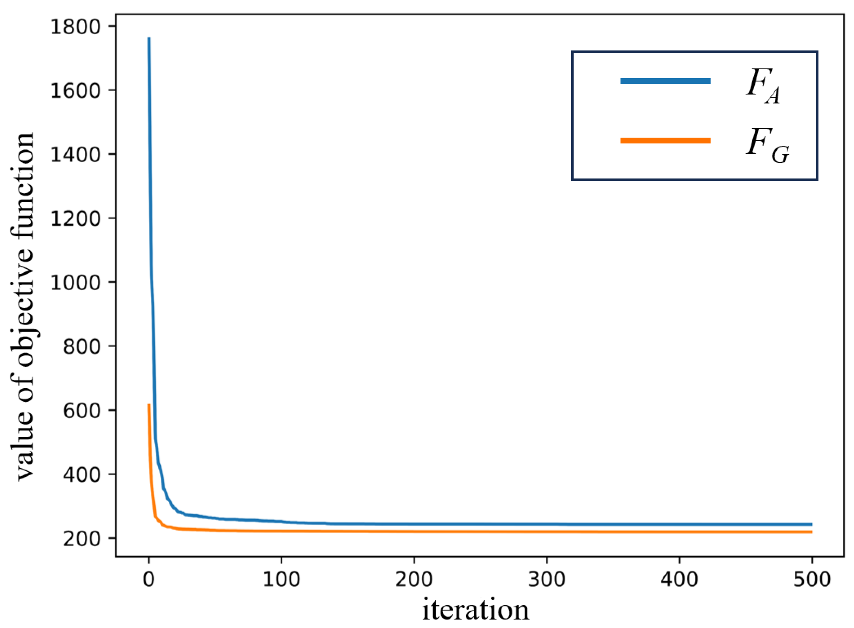
In the second stage, based on the preliminary UAVs’ path set $X^{uav}$ and the charging point set $C_{charge}$ obtained in Equation (34), we conducted an optimization resembling a TSP problem. The objective is to determine the optimal charging sequence for the UAVs to obtain the optimal path for the UGV. We will optimize the path of the UGV based on the second term of Equations (24) and (25). The optimization problem for the second stage is as follows.

$$F_G=\min [k_1·T^{ugv}+k_2·\sum _{t=1}^{T^{ugv}}{E}_{use}^{ugv}\left(t\right)]$$

(35)

$$s.t.\left\{\begin{array}{c}G\cap D=\varnothing \hfill \\ E_{init}^{ugv}-{\sum }_{x=1}^t(E_{use}^{ugv}\left(x\right)\ge 0\hfill \\ G\cap R_u=\varnothing \hfill \end{array}\right.$$

(36)

The variables in Equations (35) and (36) have been defined in Section 2. In summary, the optimization problem is to minimize the task execution time and energy consumption of the UGV, considering the obstacle avoidance constraint, energy consumption constraint, and restricted zone constraint for the UGV. We use the GA to achieve the optimal charge order $C_{charge}^{*}$ from Equation (34). Then, the A* algorithm is employed to obtain the path $X^{ugv}$ for the UGV. The A* algorithm is well suited for segmenting the UGV path planning within our two-dimensional plane.

3.2.3. Iteration

Based on the above two stages, we obtained the respective task completion durations $T^{uav}$ and $T^{ugv}$ for the UAVs and UGV. Finally, we only need to select the larger of the two to obtain the total task duration $T_{total}$ for the unmanned system by Equation (24). This completes one optimization cycle, and by iteratively repeating this process, we can achieve the desired path-planning solution.

3.3. Time Complexity

In this section, the time complexity of the proposed TAOA is evaluated and discussed. In the process of the UAVs’ path generation, the time complexity of the GA is $O(P·T)$, where P is the chromosome population of the GA and T is the total iterations of the GA. The GA is first used to calculate the charging order. The A* algorithm is then used to generate the UGV path, and the time complexity of this process is $O\left(\right|C_{charge}|·(|C_{charge}|-1))$, where $C_{charge}$ is the set of charging points. Suppose N is the maximum value among P, T, and $|C_{charge}|$, and the overall time complexity of the TAOA is $O(P·T+|C_{charge}|·(|C_{charge}|-1))\le O\left(N^2\right)$.

3.4. Summary

This section will discuss the main idea and steps of the TAOA. In general, the TAOA is based on a prediction and rolling optimization framework. Initially, the positive infinity is regarded as the result of task time $T_{total}^{*}$, and $X^{*}=\{X^{uav,*},X^{ugv,*}\}$ is regarded as the result of the unmanned system paths, of which $X^{uav,*}$ and $X^{ugv,*}$ initially are both empty sets. Meanwhile, the initial UAVs’ state $x_{uav}\left(0\right)$, the initial UGV state $x_{ugv}\left(0\right)$, the UAVs’ minimum energy threshold $\phi$, the initial iteration round $iteratio{n}_{curr}=0$, and the maximum iteration round $iteratio{n}_{max}$ are initialized. Rolling optimization is divided into three stages: UAVs’ path and charging point generation and UGV path generation and iteration. Each round, from round $iteratio{n}_{curr}$ to $iteratio{n}_{max}$, is optimized for these three stages.

In the first stage, $F_A$ in Equation (32) is optimized under the constraint (33) to obtain the UAVs’ paths $X^{uav}$ and task time $T^{uav}$. Based on the UAVs’ minimum energy threshold $\phi$, we calculate $C_{charge}$ in Equation (34) from $X^{uav}$. In the second stage, $F_G$ in Equation (35) is optimized under the constraint (36) to obtain the UGV’s path $X^{ugv}$ and task time $T^{ugv}$, based on the charging points $C_{charge}$ from the first stage. In the third stage, we calculate this round’s total task time $T_{total}$ based on $T^{uav}$ and $T^{ugv}$ in Equation (24). If $T_{total}<T_{total}^{*}$, $T_{total}^{*}$ is updated by $T_{total}$ and $X^{*}$ is updated by $\{X^{uav,*},X^{ugv,*}\}$.

The above-mentioned three stages complete the optimization of this round, and $iteratio{n}_{curr}$ is updated by $iteratio{n}_{curr}+1$. This process will continue until the end of $iteratio{n}_{curr}=iteratio{n}_{max}$. Then, the final paths of the unmanned system are obtained. Based on the above optimization scheme, we give the following pseudo-code to overview the whole process of the TAOA in Algorithm 1.

Algorithm 1: Pseudocode for the TAOA.

Input:       UAVs’ initial state $x_{uav}\left(0\right)$       UGV’s initial state $x_{ugv}\left(0\right)$       UAVs’ minimum energy threshold $\phi$       initial iteration round $iteratio{n}_{curr}$       maximum iteration round $iteratio{n}_{max}$       task time $T_{total}^{*}$       optimal path planning $X^{*}=\{X^{uav,*},X^{ugv,*}\}$ Output:       task time $T_{total}^{*}$       optimal path planning $X^{*}=\{X^{uav,*},X^{ugv,*}\}$ Initialize:       $iteratio{n}_{curr}\leftarrow 0$       $T_{total}^{*}\leftarrow \infty$       $X^{uav,*}\leftarrow \varnothing$       $X^{ugv,*}\leftarrow \varnothing$ While$iteration<iteratio{n}_{max}$Do:       Generate $X^{uav}$ and $T^{uav}$ from Equations (32) and (33)       Obtain $C_{charge}$ from $X^{uav}$ and $\phi$       Obtain $C_{charge}^{*}$ from Equation (34)       Generate $X^{ugv}$ and $T^{ugv}$ from Equations (35) and (36)       Calculate $T_{total}$ based on $T^{uav}$ and $T^{ugv}$ in Equation (24)       If $T_{total}<T_{total}^{*}$ Do:             $T_{total}^{*}\leftarrow T_{total}$             $X^{uav,*}\leftarrow X^{uav}$             $X^{ugv,*}\leftarrow X^{ugv}$

4. Results

To validate the effectiveness of the proposed TAOA, we present three sets of simulations in this section. The simulation parameters are provided in

Table 1. Experimental parameter setting.

Parameter	Value
$L_x\times L_y\times L_z$	2000 m × 2000 m × 100 m
$l_x\times l_y\times l_z$	20 m × 20 m × 10 m
$X\times Y\times Z$	$100\times 100\times 10$
$h_1$	100 m
$h_2$	60 m
$h_{max}^{uav}$	90 m
$h_{min}^{uav}$	60 m
$N_C$	2
$\Delta t$	2s
$E_{charge1}$	$1\%/\Delta t$
$E_{charge2}$	$0.002\%/\Delta t$
$E_{descend}^{uav}$	$0.5\%/\Delta t$
$E_{takeoff}^{uav}$	$1\%/\Delta t$
$E_{carry}^{ugv}$	$0.005\%/\Delta t$
$E_{throw}^{ugv}$	$0.02\%/\Delta t$
$E_{pick}^{ugv}$	$0.01\%/\Delta t$
$E_{cover}$	$0.5\%/\Delta t$
$q_1,q_2,q_3$	$1/3$
$p_d$	$0.8$
$p_f$	$0.2$
$p_{min}$	$0.7$
$p_{max}$	1
$k_1$	$0.5$
$k_2$	$0.5$
$\phi$	$20\%$
P	200
T	500
$iteratio{n}_{max}$	5000

. The hardware configuration used in the simulation was an Intel i5 processor at 2.70 GHz and 16 GB memory, and the version of the software was Python 3.8.0.

Note that the energy-related parameters given in the above table are expressed as percentages. The UGV actually consumes more power when charging than when the UAV is charged. Initially, the UAVs and UGV are at 100 percent full charge. Buildings, no-fly zones, and restricted zones were randomly arranged in the simulation scenarios specified by the above parameters.

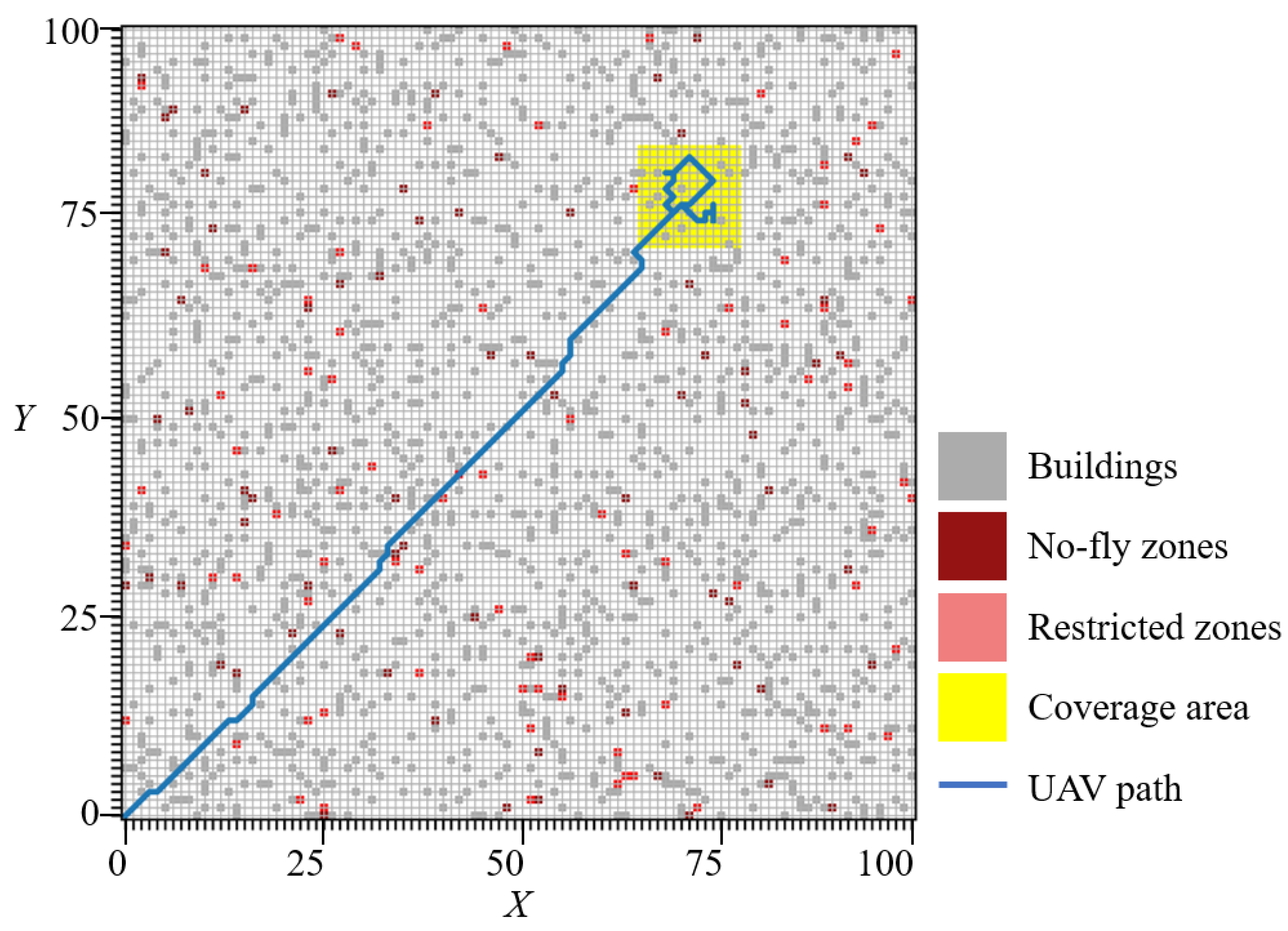
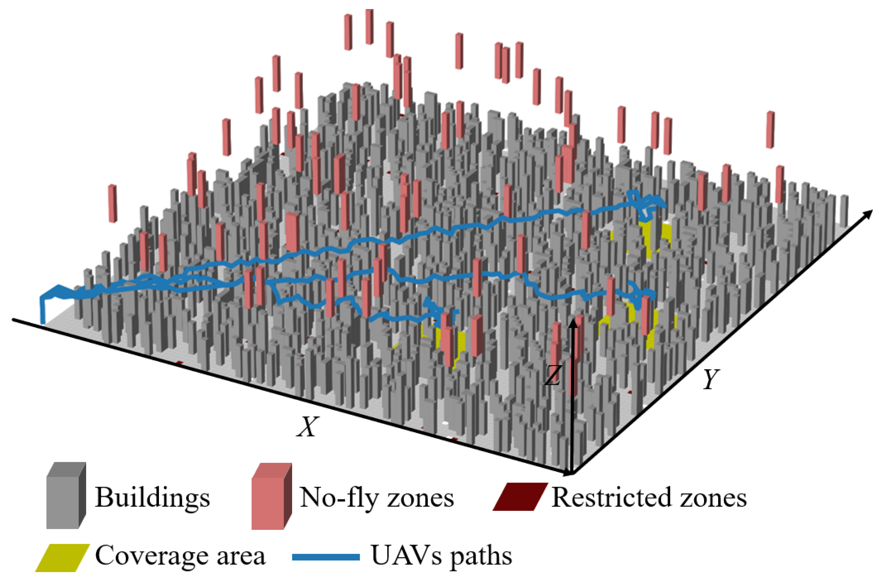
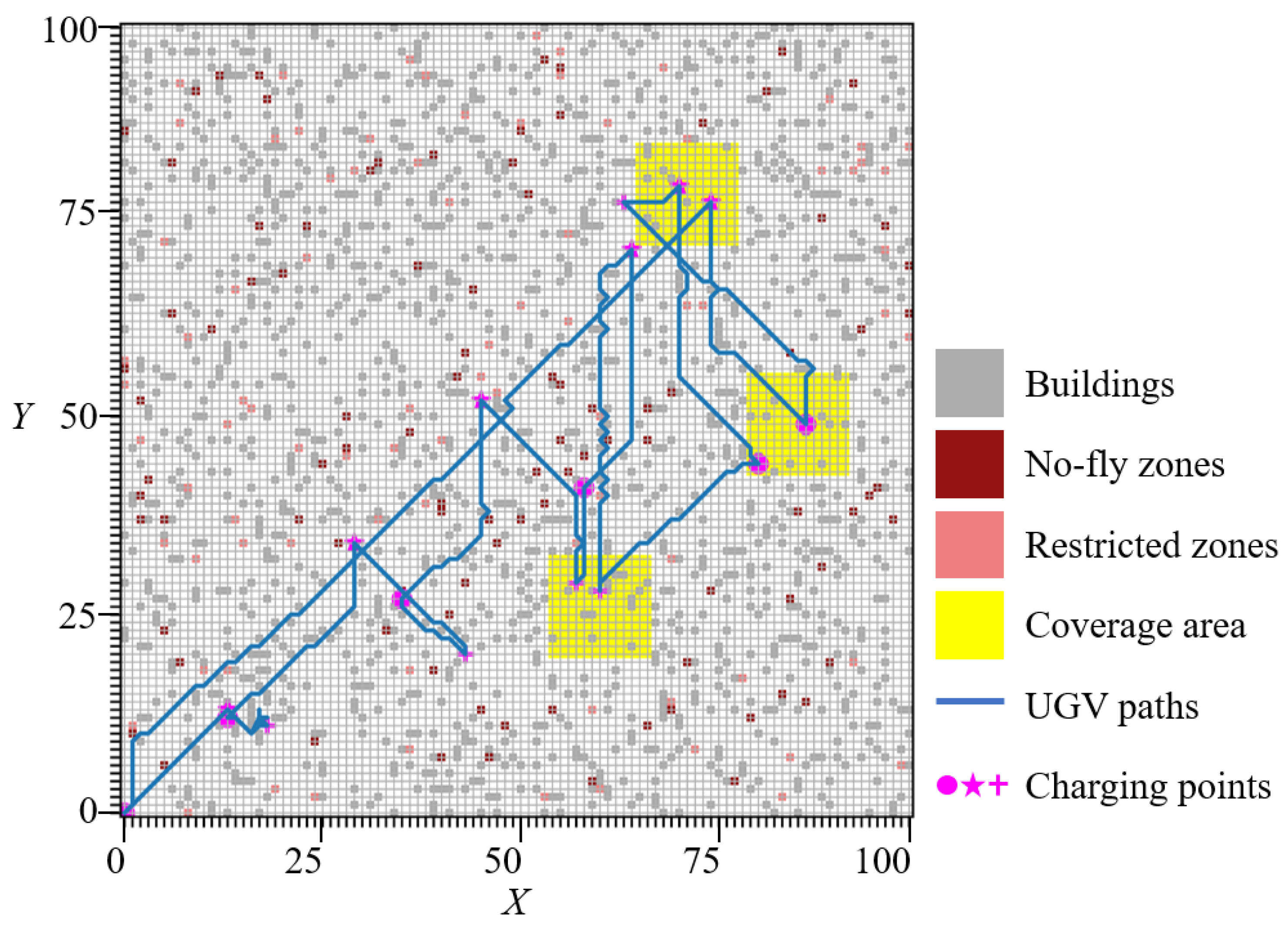
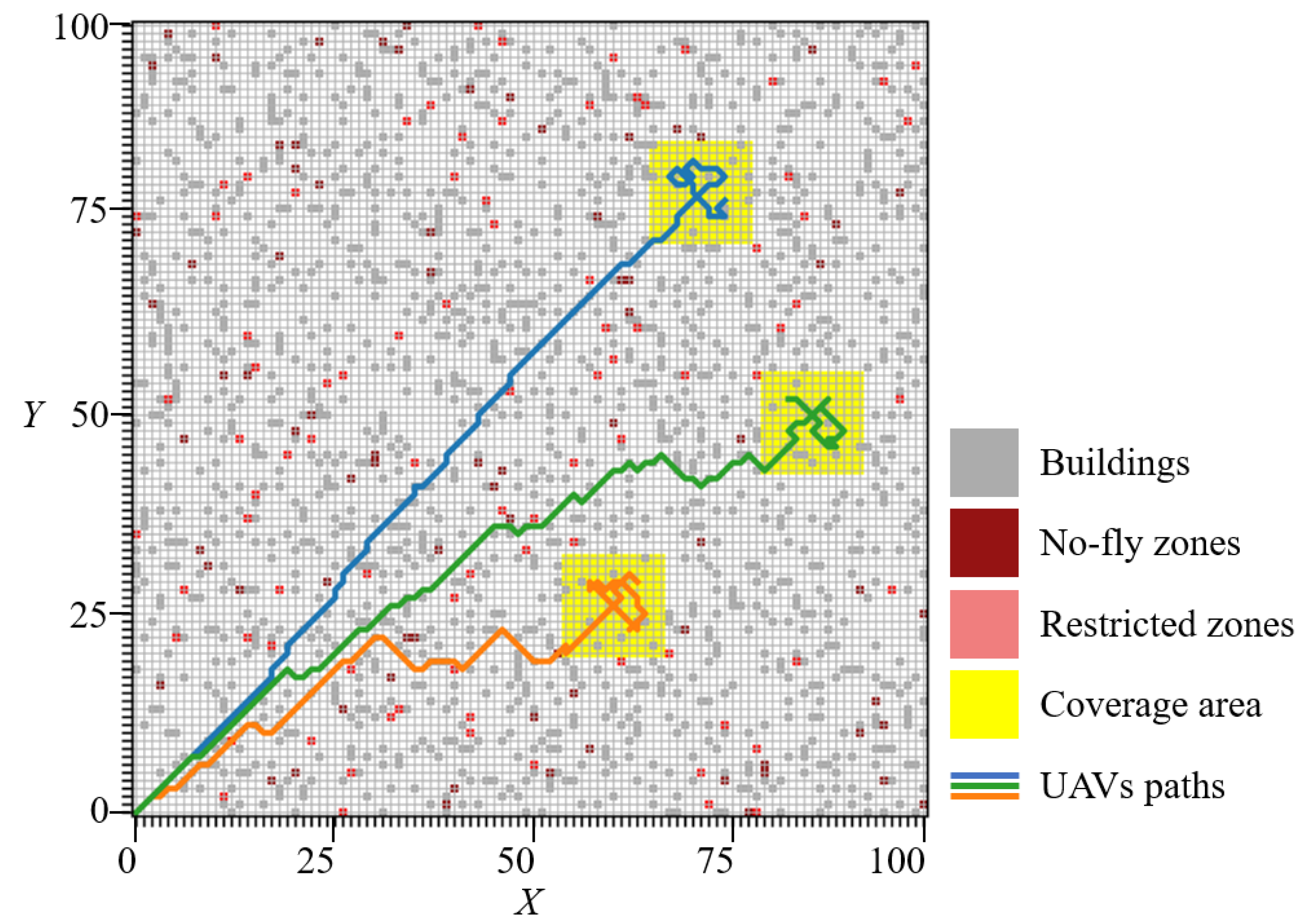
4.1. Simulation of One UAV and One UGV

This section sets up a simulation with one UAV and one UGV, both of which start at (0,0). The UAV is assigned a coverage area, which is a rectangular region, and the four vertices are (1300 m,1420 m), (1540 m,1660 m), (1540 m,1420 m), and (1300 m,1660 m). Figure 8 illustrates the two-dimensional flight trajectory of the UAV, while Figure 9 shows its three-dimensional flight trajectory. Figure 10 shows the two-dimensional driving trajectory of the UGV. The entire process took 1782 s.

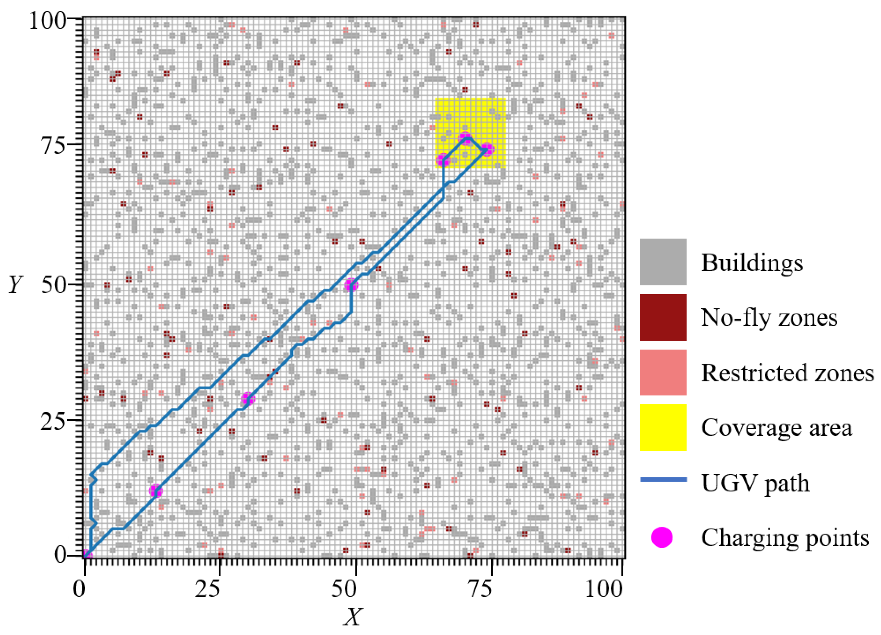
4.2. Simulation of UAVs and One UGV

In this section, three UAVs and one UGV are deployed to execute the task, with each UAV assigned a coverage area. The UAVs and UGV start at (0,0). The coverage areas are rectangular, and their vertices are shown in

Table 2. Experimental parameter setting.

Coverage Area	Vertices
Coverage area 1	(1300 m,1420 m)
	(1540 m,1660 m)
	(1540 m,1420 m)
	(1300 m,1660 m)
Coverage area 2	(1080 m,680 m)
	(1320 m,680 m)
	(1080 m,440 m)
	(1320 m,440 m)
Coverage area 3	(1620 m,1120 m)
	(1620 m,900 m)
	(1880 m,1120 m)
	(1880 m,900 m)

. Figure 11 illustrates the 2D flight trajectories of the UAVs, while Figure 12 provides a depiction of their three-dimensional flight paths. The two-dimensional driving trajectory of the UGV is shown in Figure 13. The overall execution time was 3032 s.

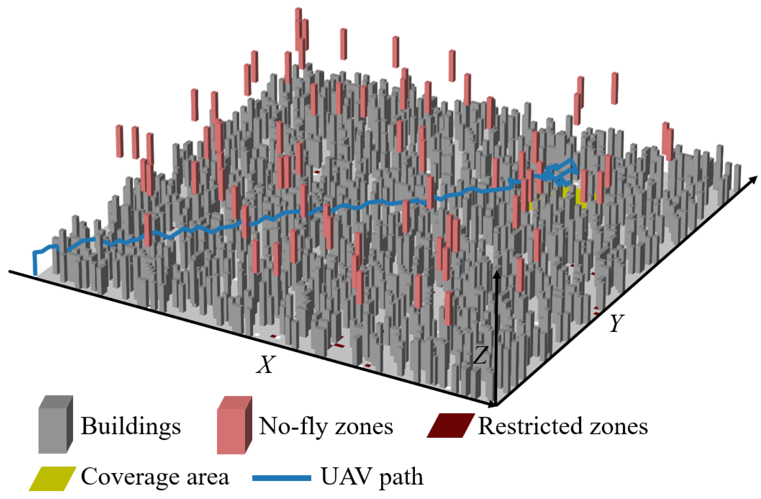
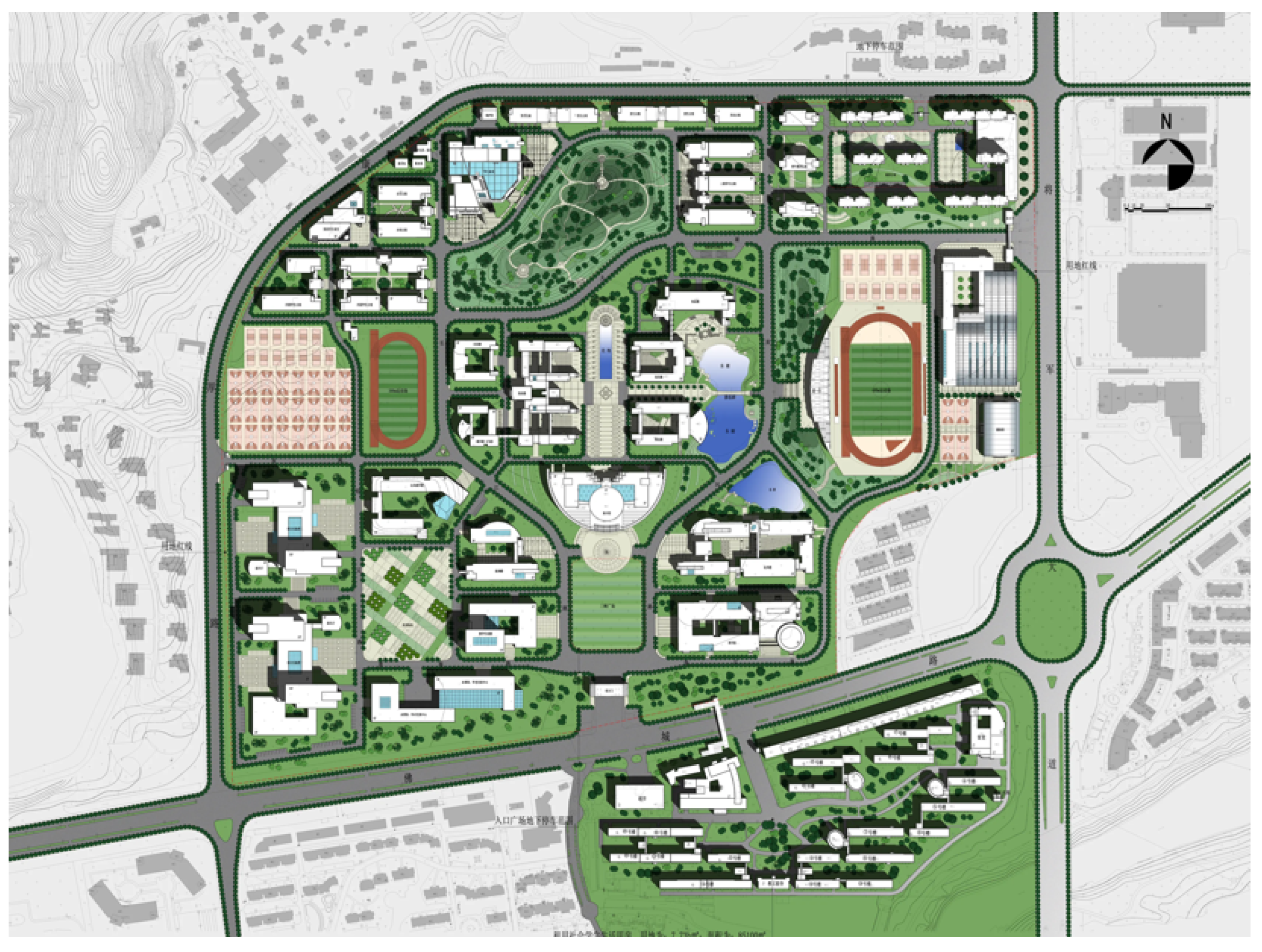
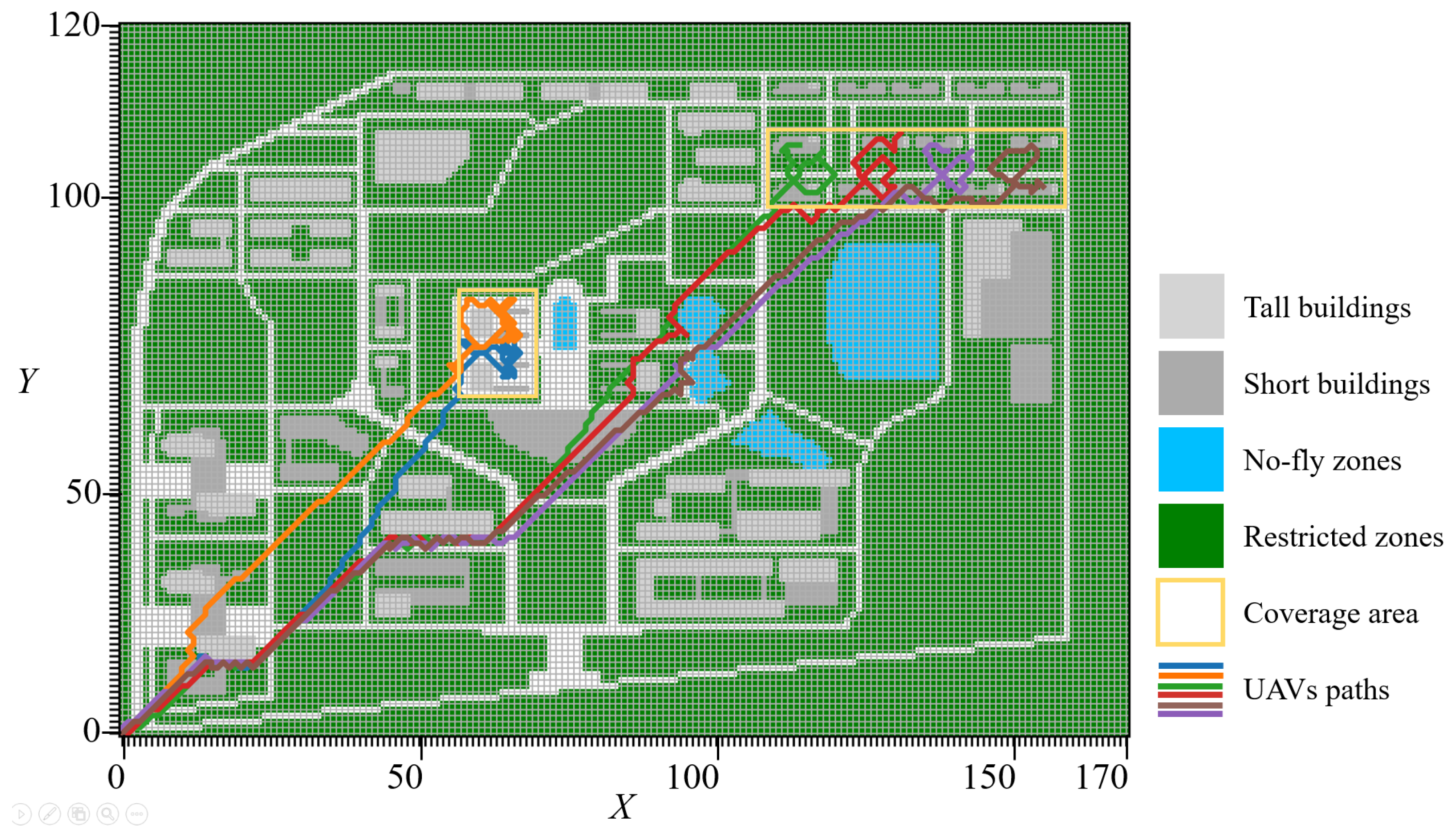
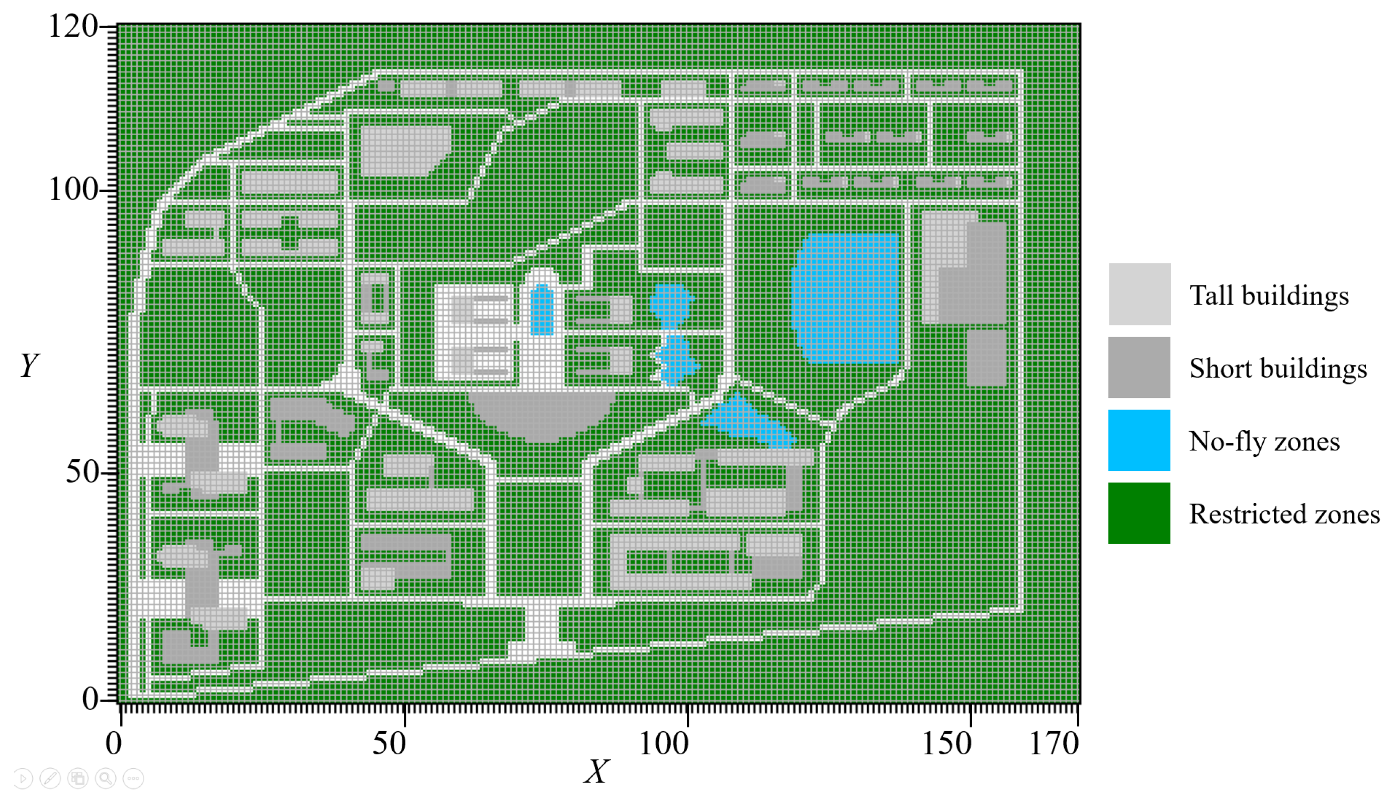
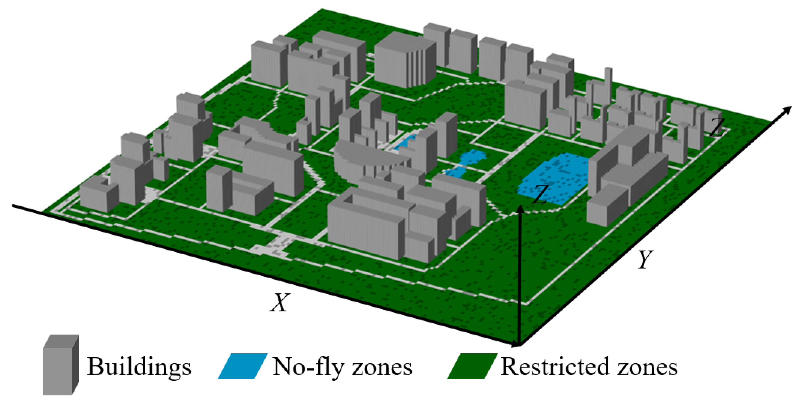
4.3. Simulation of Real-World Scenarios

This section formulates a three-dimensional synthetic scenario grounded in an authentic geographic location and subsequently validates the algorithms within it. The selected real-world scenario is the campus of Hohai University, the authors’ institution, located at longitude 118.786191 and latitude 31.913925. The campus layout is depicted in the plan view in Figure 14, from which the two-dimensional map after modeling is shown in Figure 15, and the three-dimensional map is illustrated in Figure 16. In the real scenario, green belts are designated as restricted zones for the UGV, as indicated by the green area. Areas such as water bodies and sports fields, which could affect the normal flight of the UAVs, are designated as no-fly zones and, consequently, restricted zones, depicted by the blue area. In the presence of sunlight, the reflection on the water surface can adversely affect visual localization [43], especially in windy conditions. Therefore, it is reasonable to designate water surfaces as no-fly zones. Such a configuration can minimize interference from strong light and reflections, enhancing the stability and accuracy of the visual system. This ensures that the UAVs operate in a safer and more reliable manner during task execution.

In this section, a total of six UAVs and one UGV are deployed for the task. Figure 17 illustrates the two-dimensional flight trajectories of the UAVs, while Figure 18 depicts the three-dimensional flight paths of the UAVs. Additionally, Figure 19 displays the two-dimensional driving trajectory of the UGV. The overall execution time was 3832 s. Figure 20 shows the convergence curve after averaging 30 independently repeated experiments under the scenario setup in this section.

5. Discussion

5.1. Feasibility and Effectiveness

From the results in Section 4.1, it can be observed that the UAV is capable of navigating through our synthetic urban environment, avoiding randomly generated buildings and no-fly zones. The UAV efficiently reached the designated coverage start position, completing area coverage as quickly as possible. The UGV successfully retrieved and charged the UAV before its energy level dropped below the threshold. Ultimately, the UGV returned with the UAV. The UGV demonstrates effective obstacle avoidance during the process of UAV retrieval and transportation, considering both buildings and restricted areas.

The scaling up of UAVs poses challenges for the charging and carrying optimization of the UGV for the UAV swarm in Section 4.2. As we can see, the UGV can sequentially retrieve and charge each UAV at its designated charging point and ensure that it avoids obstacles along the way. Ultimately, the UGV returns with the UAVs. The UGV demonstrates effective obstacle avoidance during the process of UAV retrieval and transportation, considering both buildings and restricted areas. This demonstrates the adaptability of the UGV to the scale of the UAV swarm.

The experimental results of the above two sections verify the feasibility and effectiveness of TAOA algorithm in collaborative path planning in urban environment.

5.2. Applicability in Real-World Scenarios

In Section 4.3, simulation under real-world scenarios are conducted to verify the applicability of the proposed model and method in practical applications. In Figure 17 and Figure 18, it is clear that the UAVs initiate their journey from the starting point, navigating autonomously towards the designated coverage area. Evading obstacles and steering clear of no-fly zones along their trajectory, each UAV finally accomplishes coverage detection within its assigned areas. In Figure 19, the UGV travels to various charging points to provide the UAVs with the capability to continue their missions. Importantly, all charging points are strategically positioned along the feasible path of the UGV, ensuring that the flight conditions for the UAVs are met. At the end of the mission, all the UAVs are retrieved by the UGV. As we can see in Figure 20, both the $F_A$ and $F_G$ functions in the two stages of the TAOA can converge quickly within 100 iterations and tend to a fixed value, which shows that the TAOA has the guarantee of convergence. By conducting experiments in a real-world scenario-mapped environment model in Section 4.3, the practical application prospects of TAOA algorithm in collaborative path planning problems are verified.

5.3. Summary

The experimental results highlight the stability of UAVs when navigating through a simulated urban environment. This navigation involves successfully avoiding obstacles such as randomly generated buildings and designated no-fly zones. Notably, the UAVs efficiently reached their designated waypoints, ensuring swift area coverage.

Furthermore, the role of UGVs is emphasized in sequentially retrieving and charging each UAV at their assigned charging points. These points are strategically planned to prevent the UAVs’ energy levels from dropping below a predefined threshold. This underscores the importance of minimizing task duration and demonstrates the system’s efficiency. The UGV effectively avoids obstacles during UAV retrieval and deployment, considering both buildings and restricted areas.

By focusing on overall execution time, the importance of optimizing task duration as a key performance metric is highlighted in evaluating system efficiency and effectiveness. The simulation results and discussion reveal the intricate coordination and efficiency achieved within the system, demonstrating successful mission objective execution by both UAVs and UGVs. The seamless interaction within the unmanned system validates the effectiveness of the proposed approach in real-world scenarios.

6. Conclusions

In this study, the modeling of and a method for path planning in collaborative coverage monitoring for urban scenarios are proposed. This study designs a realistic and convincing model of an urban scenario and introduces a UGV into the model to solve the endurance problem of the UAVs in this long-time task scenario. The UAVs and UGV constitute a heterogeneous unmanned system to collaboratively solve the path-planning problem in the model. Building upon this model, this paper designs a Three-stage Alternating Optimization Algorithm (TAOA), involving two steps of prediction and rolling optimization. A three-stage scheme is introduced to the rolling optimization to effectively address the complex optimization process for the unmanned system, including of UAVs’ path and charging point generation, the UGV’s path generation, and the iteration. In order to verify the performance of the proposed model and method, this paper conducts simulations in a pre-constructed simulation scene and an environment mapped using a real-world scenario. This confirms the feasibility of the proposed method.

Future endeavors will focus on advancing this model’s efficiency, with an emphasis on elevating its real-time ability and exploring possibilities for its application in real urban scenarios.

References

1. Casper, J.; Murphy, R. Human-robot interactions during the robot assisted urban search and rescue response at the world trade center. IEEE Trans. Syst. Man Cybernetics. Part B Cybern. A Publ. IEEE Syst. Man Cybern. Soc. 2003, 33, 367–385. [Google Scholar] [CrossRef] [PubMed]
2. Yin, C.; Xiao, Z.; Cao, X.; Xi, X.; Yang, P.; Wu, D. Offline and online search: UAV multiobjective path planning under dynamic urban environment. IEEE Internet Things J. 2018, 5, 546–558. [Google Scholar] [CrossRef]
3. Cao, C.; Zhang, J.; Travers, M.; Choset, H. Hierarchical coverage path planning in complex 3d environments. In Proceedings of the 2020 IEEE International Conference on Robotics and Automation, Paris, France, 31 May–31 August 2020; Volume 5, pp. 3206–3212. [Google Scholar]
4. Chen, Y.; Yang, D.; Yu, J. Multi-UAV task assignment with parameter and time-sensitive uncertainties using modified two-part wolf pack search algorithm. IEEE Trans. Aerosp. Electron. Syst. 2018, 54, 2853–2872. [Google Scholar] [CrossRef]
5. Li, L.; Gu, Q.; Liu, L. Research on path planning algorithm for multi-UAV maritime targets search based on genetic algorithm. In Proceedings of the 2020 IEEE International Conference on Information Technology, Big Data and Artificial Intelligence (ICIBA), Chongqing, China, 6–8 November 2020; pp. 840–843. [Google Scholar]
6. Papaioannou, S.; Kolios, P.; Theocharides, T.; Panayiotou, C.G.; Polycarpou, M.M. Integrated ray-tracing and coverage planning control using reinforcement learning. In Proceedings of the 2022 IEEE 61st Conference on Decision and Control, Cancun, Mexico, 6–9 December 2022; pp. 7200–7207. [Google Scholar]
7. Theile, M.; Bayerlein, H.; Nai, R.; Gesbert, D.; Caccamo, M. UAV coverage path planning under varying power constraints using deep reinforcement learning. In Proceedings of the 2020 IEEE/RSJ International Conference on Intelligent Robots and Systems, Las Vegas, NV, USA, 24 October 2020–24 January 2021; pp. 1444–1449. [Google Scholar]
8. Tolstaya, E.; Paulos, J.; Kumar, V.; Ribeiro, A. Multi-robot coverage and exploration using spatial graph neural networks. In Proceedings of the 2021 IEEE/RSJ International Conference on Intelligent Robots and Systems, Prague, Czech Republic, 27 September–1 October 2021; pp. 8944–8950. [Google Scholar]
9. Papaioannou, S.; Kolios, P.; Theocharides, T.; Panayiotou, C.G.; Polycarpou, M.M. Cooperative receding horizon 3D coverage control with a team of networked aerial agents. In Proceedings of the 2023 62nd IEEE Conference on Decision and Control, Singapore, 13–15 December 2023; pp. 4399–4404. [Google Scholar]
10. Choi, Y.; Briceno, S.; Mavris, D.N. Energy-constrained multi-UAV coverage path planning for an aerial imagery mission using column generation. J. Intell. Robot. Syst. Theory Appl. 2020, 97, 125–139. [Google Scholar] [CrossRef]
11. Papaioannou, S.; Kolios, P.; Theocharides, T.; Panayiotou, C.G.; Polycarpou, M.M. Distributed search planning in 3-D environments with a dynamically varying number of agents. IEEE Trans. Syst. Man Cybern. Syst. 2023, 53, 4117–4130. [Google Scholar] [CrossRef]
12. Chen, J.; Du, C.; Zhang, Y.; Han, P.; Wei, W. A clustering-based coverage path planning method for autonomous heterogeneous UAVs. IEEE Trans. Intell. Transp. Syst. 2022, 23, 25546–25556. [Google Scholar] [CrossRef]
13. Papaioannou, S.; Kolios, P.; Theocharides, T.; Panayiotou, C.G.; Polycarpou, M.M. Integrated guidance and gimbal control for coverage planning with visibility constraints. IEEE Trans. Aerosp. Electron. Syst. 2023, 59, 1276–1291. [Google Scholar] [CrossRef]
14. Misra, S.; Biswas, S.; Minai, A.A.; Sharma, R. Cooperative search area optimization using multiple unmanned aerial vehicles in a GPS-denied environment. In Proceedings of the International Conference on Unmanned Aircraft Systems, Atlanta, GA, USA, 11–14 June 2019; pp. 580–587. [Google Scholar]
15. Zhang, X.; Duan, H. An improved constrained differential evolution algorithm for unmanned aerial vehicle global route planning. Appl. Soft Comput. 2015, 26, 270–284. [Google Scholar] [CrossRef]
16. Zhen, Z.; Chen, Y.; Wen, L.; Han, B. An intelligent cooperative mission planning scheme of UAV swarm in uncertain dynamic environment. Aerosp. Sci. Technol. 2020, 100, 105826. [Google Scholar] [CrossRef]
17. Chen, J.; Ling, F.; Zhang, Y.; You, T.; Liu, Y.; Du, X. Coverage path planning of heterogeneous unmanned aerial vehicles based on ant colony system. Swarm Evol. Comput. 2022, 69, 101005. [Google Scholar] [CrossRef]
18. Gao, L.; Han, Z.; Hong, D.; Zhang, B.; Chanussot, J. CyCU-Net: Cycle-consistency unmixing network by learning cascaded autoencoders. IEEE Trans. Geosci. Remote. Sens. 2022, 60, 5503914. [Google Scholar] [CrossRef]
19. Gao, L.; Li, J.; Zheng, K.; Jia, X. Enhanced autoencoders with attention-embedded degradation learning for unsupervised hyperspectral image super-resolution. IEEE Trans. Geosci. Remote. Sens. 2023, 61, 5509417. [Google Scholar] [CrossRef]
20. Su, Y.; Gao, L.; Jiang, M.; Plaza, A.; Sun, X.; Zhang, B. NSCKL: Normalized spectral clustering with kernel-based learning for semisupervised hyperspectral image classification. IEEE Trans. Cybern. 2023, 53, 6649–6662. [Google Scholar] [CrossRef] [PubMed]
21. Yao, P.; Wang, H.; Ji, H. Multi-UAVs tracking target in urban environment by model predictive control and improved grey wolf optimizer. Aerosp. Sci. Technol. 2016, 55, 131–143. [Google Scholar] [CrossRef]
22. Riehl, J.R.; Collins, G.E.; Hespanha, J.P. Cooperative search by UAV teams: A model predictive approach using dynamic graphs. IEEE Trans. Aerosp. Electron. Syst. 2011, 47, 2637–2656. [Google Scholar] [CrossRef]
23. Huang, L.; Qu, H.; Ji, P.; Liu, X.; Fan, Z. A novel coordinated path planning method using k-degree smoothing for multi-UAVs. Appl. Soft Comput. 2016, 48, 182–192. [Google Scholar] [CrossRef]
24. Wu, Y.; Wu, S.; Hu, X. Cooperative path planning of UAVs & UGVs for a persistent surveillance task in urban environments. IEEE Internet Things J. 2021, 8, 4906–4919. [Google Scholar]
25. Wang, J.; Wu, Z.; Yan, S.; Tan, M.; Yu, J. Real-time path planning and following of a gliding robotic dolphin within a hierarchical framework. IEEE Trans. Veh. Technol. 2021, 70, 3243–3255. [Google Scholar] [CrossRef]
26. Wu, N.; Chacon, C.; Hakl, Z.; Petty, K.; Smith, D. Design and implementation of an unmanned aerial and ground vehicle recharging system. In Proceedings of the 2019 IEEE National Aerospace and Electronics Conference (NAECON), Dayton, OH, USA, 15–19 July 2019. [Google Scholar]
27. Grocholsky, B.; Keller, J.; Kumar, V.; Pappas, G. Cooperative air and ground surveillance. IEEE Robot. Autom. Mag. 2006, 13, 16–25. [Google Scholar] [CrossRef]
28. Minaeian, S.; Liu, J.; Son, Y.J. Vision-Based Target Detection and Localization via a Team of Cooperative UAV and UGVs. IEEE Trans. Syst. Man Cybern. Syst. 2016, 46, 1005–1016. [Google Scholar] [CrossRef]
29. Ghamry, K.A.; Kamel, M.A.; Zhang, Y. Cooperative forest monitoring and fire detection using a team of UAVs-UGVs. In Proceedings of the International Conference on Unmanned Aircraft Systems, Arlington, VA, USA, 7–10 June 2016. [Google Scholar]
30. Qin, H.; Meng, Z.; Meng, W.; Chen, X.; Sun, H.; Lin, F.; Ang, M.H. Autonomous exploration and mapping system using heterogeneous UAVs and UGVs in GPS-denied environments. IEEE Trans. Veh. Technol. 2018, 68, 1339–1350. [Google Scholar] [CrossRef]
31. Lakas, A.; Belkhouche, B.; Benkraouda, O.; Shuaib, A.; Alasmawi, H.J. A framework for a cooperative UAV-UGV system for path discovery and planning. In Proceedings of the 2018 International Conference on Innovations in Information Technology (IIT), Al Ain, United Arab Emirates, 18–19 November 2018. [Google Scholar]
32. Asadi, K.; Suresh, A.K.; Ender, A.; Gotad, S.; Maniyar, S.; An, S.; Noghabaei, M.; Han, K.; Lobaton, E.; Wu, T. An integrated UGV-UAV system for construction site data collection. Autom. Constr. 2020, 112, 103068. [Google Scholar] [CrossRef]
33. Wei, Y.; Qiu, H.; Liu, Y.; Du, J.; Pun, M.O. Unmanned aerial vehicle (UAV)-assisted unmanned ground vehicle (UGV) systems design, implementation and optimization. In Proceedings of the 2017 3rd IEEE International Conference on Computer and Communications (ICCC), Chengdu, China, 13–16 December 2017. [Google Scholar]
34. Li, J.; Deng, G.; Luo, C.; Lin, Q.; Yan, Q.; Ming, Z. A hybrid path planning method in unmanned air/ground vehicle (UAV/UGV) cooperative systems. IEEE Trans. Veh. Technol. 2016, 65, 9585–9596. [Google Scholar] [CrossRef]
35. Li, J.; Sun, T.; Huang, X.; Ma, L.; Lin, Q.; Chen, J.; Leung, V.C. A memetic path planning algorithm for unmanned air/ground vehicle cooperative detection systems. IEEE Trans. Autom. Sci. Eng. 2021, 99, 1–14. [Google Scholar] [CrossRef]
36. Yu, W.; Liu, J.; Zhou, J. A novel sparrow particle swarm algorithm (SPSA) for unmanned aerial vehicle path planning. Sci. Program. 2021, 2021, 5158304. [Google Scholar] [CrossRef]
37. Niu, G.; Yang, Q.; Gao, Y.; Pun, M.O. Vision-based autonomous landing for unmanned aerial and ground vehicles cooperative systems. IEEE Robot. Autom. Lett. 2022, 3, 6234–6241. [Google Scholar] [CrossRef]
38. Ropero, F.; Muñoz, P.; R-Moreno, M.D. TERRA: A path planning algorithm for cooperative UGV–UAV exploration. Eng. Appl. Artif. Intell. 2019, 78, 260–272. [Google Scholar] [CrossRef]
39. Zheng, J.; Ding, M.; Sun, L.; Liu, H. Distributed stochastic algorithm based on enhanced genetic algorithm for path planning of multi-UAV cooperative area search. IEEE Trans. Intell. Transp. Syst. 2023, 24, 8290–8303. [Google Scholar] [CrossRef]
40. Zhong, M.; Cassandras, C.G. Distributed coverage control and data collection with mobile sensor networks. IEEE Trans. Autom. Control 2011, 56, 2445–2455. [Google Scholar] [CrossRef]
41. Hu, J.; Xie, L.; Lum, K.Y.; Xu, J. Multi-agent information fusion and cooperative control in target search. EEE Trans. Control Syst. Technol. 2013, 21, 1223–1235. [Google Scholar] [CrossRef]
42. Xiao, L.; Boyd, S.; Lall, S. A scheme for robust distributed sensor fusion based on average consensus In Proceedings of the IPSN 2005. Fourth International Symposium on Information Processing in Sensor Networks on 2005, Boise, ID, USA, 15 April 2005; pp. 63–70. [Google Scholar]
43. Gao, L.; Wang, Z.; Zhuang, L.; Yu, H.; Zhang, B.; Chanussot, J. Using low-rank representation of abundance maps and nonnegative tensor factorization for hyperspectral nonlinear unmixing. IEEE Trans. Geosci. Remote Sens. 2022, 60, 5504017. [Google Scholar] [CrossRef]
Figure 1. UAV and UGV path-planning simulation scene schematic diagram.
Remotesensing 16 01152 g001
Figure 2. Schematic diagram of UAV.
Remotesensing 16 01152 g002
Figure 3. Schematic diagram of UGV.
Remotesensing 16 01152 g003
Figure 4. Coverage range of the UAV at a validated altitude in case (a) of occlusion.
Remotesensing 16 01152 g004
Figure 5. Coverage range of the UAV at a validated altitude in case (b) of occlusion.
Remotesensing 16 01152 g005
Figure 6. Coverage range of the UAV at a validated altitude in case (c) of occlusion.
Remotesensing 16 01152 g006
Figure 7. Coverage range of the UAV at a validated altitude in case (d) of occlusion.
Remotesensing 16 01152 g007
Figure 8. Two-dimensional UAV route of path-planning results.
Remotesensing 16 01152 g008
Figure 9. Three-dimensional UAV route of path-planning results.
Remotesensing 16 01152 g009
Figure 10. Two-dimensional UGV route of path-planning results.
Remotesensing 16 01152 g010
Figure 11. Two-dimensional UAVs routes of path-planning results.
Remotesensing 16 01152 g011
Figure 12. Three-dimensional UAVs routes of path-planning results.
Remotesensing 16 01152 g012
Figure 13. Two-dimensional UGV route of path-planning results.
Remotesensing 16 01152 g013
Figure 14. Actual scene plane map, longitude 118.786191 and latitude 31.913925.
Remotesensing 16 01152 g014
Figure 15. Two-dimensional diagram of simulation scene based on actual scene modeling.
Remotesensing 16 01152 g015
Figure 16. Three-dimensional diagram of simulation scene based on actual scene modeling.
Remotesensing 16 01152 g016
Figure 17. Two-dimensional UAV routes of path-planning results.
Remotesensing 16 01152 g017
Figure 18. Three-dimensional UAV routes of path-planning results.
Remotesensing 16 01152 g018
Figure 19. Two-dimensional UGV route of path-planning results.
Remotesensing 16 01152 g019
Figure 20. The convergence curve after averaging 30 independently repeated experiments.
Remotesensing 16 01152 g020