Abstract
This paper introduces a model-independent passive source localization method, employing asynchronous distributed hydrophones in shallow water. Based on the frequency invariability of the acoustic field, assuming the correct source range information, the warped spectra of received signals at distributed hydrophones exhibit identical shapes. Subsequently, a cost function is formulated to mutually align the warped spectra, with its maximum point indicating the source location. The proposed method can locate the source in two-dimensional horizontal space without requiring either angle- or time-synchronization information. Numerical simulations are conducted to demonstrate the performance of the proposed method.
1. Introduction
In shallow water, passive source localization remains a topic of ongoing interest and concern for many researchers. One classical method for addressing this issue is matched field processing (MFP) [1], where the received acoustic field is matched with model-calculated replicas to determine the source location based on the best matching point. However, despite its effectiveness, the performance of MFP significantly degrades if the environment model used for replica calculation is mismatched. Additionally, this class of methods requires a large-aperture array comparable to the water depth to adequately sample the acoustic field, thereby limiting its practical application. These limitations of MFP have spurred the development of model-independent localization methods.
In shallow water, normal mode theory is commonly employed to explain low-frequency sound propagation, where the received field can be described as the summation of a series of normal modes [2]. The interference characteristics among these modes contain information about the ocean environment and the source location. As a result, the source can be located by exploiting the interference characteristics among the modes. The methods of source localization in shallow water could be broadly categorized into two groups: (1) waveguide invariant [3] or array invariant-based methods [4,5,6] and (2) warping transform-based methods [7,8,9]. The first category estimates the source range based on the relationship between the source range and the value of the waveguide/array invariant, with the waveguide invariant obtained as a priori environmental information. The second category, warping transform-based methods, utilize the invariability of the characteristic frequency of the normal modes and determines the source range by matching the measured and standard warped spectra. In this localization process, the standard warped spectrum must be obtained in advance by using a guide source at a known range. Both types of methods can estimate the source range without requiring sound propagation modeling. However, the majority of existing methods are designed for a single receiving platform and focus on locating the source in range space. Additionally, some a priori information (e.g., the value of waveguide invariant or a guide source) is required. However, a two-dimensional (2D) location (i.e., both x and y coordinates) is unquestionably more useful than range information in practical applications such as attack, communication, and monitoring. To achieve 2D localization, an additional array with a horizontal aperture can be used to determine the azimuthal angle of the source. Another effective approach is to observe the source using spatially distributed hydrophones. In this case, information about the mode interference characteristics is sufficient for 2D localization.
Passive localization using distributed sensors has been extensively studied. A traditional methodology for this task involves combining the target’s direction of arrival (DOA) measured by the distributed sensors [10,11,12,13,14,15,16]. The cost function can be constructed using these measured bearings to derive the source position. Weighted least-squares (WLS) methods [10,11,12] and maximum likelihood methods [13] are commonly used to solve this problem. Another common approach for this task involves measuring the time differences of the sensors [17,18,19,20,21,22]; then, the source position can be solved by intersecting a set of hyperbolic curves [17]. However, most of the algorithms mentioned above are derived under free-field and plane-wave assumptions, which may lead to performance degradation in practical shallow water environments. Specifically, the measured angle of arrival (AOA) for a horizontal line array could deviate from the true counterpart due to boundary reflections, rendering AOA-based methods biased or invalid. For the time difference of arrival-based algorithms, the primary challenge is clock synchronization among the distributed sensors. Additionally, performance degradation can occur due to time-delay estimation errors and sound speed mismatches in practical applications. In shallow water, propagation time differences between individual modes can be utilized to locate broadband sources using distributed hydrophones [23,24]. Benefitting from the stability of the acoustic field, this kind of algorithm can locate sources without either angle or time synchronization information. However, this algorithm requires separating propagation modes and determining their arrival times, which discourages its practical application.
This paper introduces a passive model-independent source localization method based on several spatially distributed hydrophones in shallow water. The proposed method determines the 2D source location based on the invariability of the characteristic frequency of the normal modes, thus neither the angle nor time synchronization information is required. Compared to the method in Ref. [23], the proposed method introduces the warping transform of the autocorrelation function (ACF) and directly utilizes the warped spectra to construct the cost function, simplifying its implementation in practice and extending its applicability to non-impulse sources. Specifically, for an assumed source location, the method applies the warping transform to the ACF of the received signal of each hydrophone and calculates the cost function by mutually matching the warped spectra from different hydrophones. Due to the invariability of the characteristic frequency of the acoustic field, the warped spectra from different hydrophones will have the same shape if the correct source location is assumed, enabling the maximum point of the cost function to indicate the source location. The main innovations of the method in this paper are as follows: (1) The proposed method is able to achieve source localization by exploiting the acoustic field feature without either the angle- or time-synchronization information. (2) The proposed method works on the signal autocorrelation rather than on the raw signal. Numerical simulations are conducted in a shallow water environment to analyze the performance of the proposed method. The results can be summarized as the following two points. Firstly, the proposed method performs as expected when the received field is dominated by the reflected modes but may be seriously degraded when the refracted modes dominate the received field. Secondly, the source in the detection area (i.e., the area enclosed by the connection line of the hydrophones) can be located unambiguously when the hydrophones are deployed as a regular polygon.
The remainder of this paper is organized as follows: The basic theories are presented in Section 2. In Section 3, the principle and the localization procedures are described. Numerical simulations and corresponding performance analysis are presented in Section 4, followed by a short conclusion in Section 5.
2. Basic Theory
2.1. Application Scene and Normal Mode Theory
The application scene is illustrated in Figure 1, where M distributed hydrophones are deployed at a common depth to record the signal radiated from a remote broadband source. The source is located at ps = [xs, ys, zs]T. The emitting signal of the source is denoted as s(t) in the time domain and S(f) in the frequency domain. One assumes that the location of the mth hydrophone is pm = [xm, ym, zr]T, in which zr (positive downwards) denotes the common receiver depth. The received signal of the mth hydrophone can be denoted as xm(t) in the time domain and pm(f) in the frequency domain. What we need to do is to estimate [xs, ys]T based on the observed acoustic field xm(t) [or pm(f)], m = 1, 2, …, M, without either the angle- or time-synchronization information.
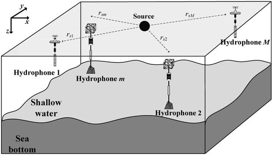
Figure 1.
Application scene.
According to normal mode theory, the received field in shallow water can be expressed by a superposition of a series of normal modes. Under the specific boundary conditions, the eigenvalue and the eigenfunction of the normal mode can be determined by solving the wave equation. The received field pm(rsm, zm, f) on the mth hydrophone in the range-independent environment can be expressed as follows [2]:
where N denotes the number of the propagation modes, krn(f) and ψn(z) denote the eigenvalue (horizontal wavenumber) and eigenfunction (mode depth function) of the nth mode, respectively, and Amn(f) is the mode amplitude.
The medium density around the source is denoted as ρ(zs), and rsm is the horizontal range between the source and the mth hydrophone.
2.2. Warping Transform of the Autocorrelation Function
On the basis of the normal mode representation [illustrated in Equation (1)], the ACF of the received field on the mth hydrophone can be shown as:
Equation (4) contains the self-interference terms (n = k) and the cross-interference terms (n ≠ k). The unilateral ACF (referred to as ACF below) is introduced herein to eliminate the useless self-interference terms [8], which is defined as:
where
In Equation (5), tm0 = rsm/c is the propagation time, c is the sound speed, vn is the characteristic frequency of the nth mode, μl denotes the interference characteristic frequency between the nth and kth mode, denotes the number of the possible combinations, and the superscript * denotes the complex conjugation operation.
As seen in Equation (5), the time-dependent phase of the signal ACF is . Given a known source location, the warping transform in the time domain can be applied to , based on the resampling function.
The output can be shown as:
It is obviously shown in Equation (8) that the spectrum of the warped ACF (named as FTWT spectrum) supplies a stationary monochromatic output with the intrinsic frequency μl. Here, the interference characteristic frequency μl also bears the property of frequency invariability [8].
As shown in Equation (7), source range is involved in the warping transform. Actually, if the source range is correctly given, the obtained interference characteristic frequencies will only be determined by the environment and is independent of the source-receiver geometry. On the contrary, with the wrong source range information, the obtained interference characteristic frequencies will deviate from the standard values. Following the conclusions in Ref. [8], if the true source range is rs, while one conducts the warping transform with an assumed range ra, then the obtained FTWT spectrum will peak at the biased interference characteristic frequencies as follows:
where μl is the standard interference characteristic frequencies, which only relates to the environment, and μal is the biased counterpart when using the incorrect source range in Equation (7).
3. Proposed Localization Method
In the case that the source is detected by multiple spatially distributed hydrophones simultaneously, its location can then be determined by mutually matching the FTWT spectra from different hydrophones. Specifically, assuming a source location psa = [xsa, ysa]T (depth coordinates of the source and sensors omitted for brevity), one can calculate its ranges to the distributed hydrophones and then apply the warping transform to the ACF of each hydrophone. If the assumed source location is correct, the characteristics of the obtained FTWT spectra obtained from different hydrophones should be consistent, as all hydrophones can extract standard interference characteristic frequencies determined solely by the environment. Otherwise, if the assumed source location is incorrect, the abovementioned consistency will be disrupted. In other words, the accuracy of an assumed source location can be assessed by evaluating the consistency of the FTWT spectra from different hydrophones. The cost function is constructed as:
where psa is the assumed source location, denotes the FTWT spectrum for the mth hydrophone that can be calculated by applying Fourier/wavelet transform to the corresponding warping output , and ||·|| is the Euclidean norm.
Overall, the proposed method can be summarized in the following seven steps:
- (1)
- Deploy M hydrophones at a common depth to record the signal radiated by a broadband source. The location and received signal of the mth hydrophone are denoted as pm = [xm, ym]T and xm(t), respectively;
- (2)
- Calculate the unilateral ACF denoted as ;
- (3)
- Divide the area of interest into grid points, denoted as [xi, yj], i = 1, 2, …, Lx, j = 1, 2, …, Ly, where Lx and Ly are the number of the grid on the x and y axes, respectively;
- (4)
- Calculate the range between psa and pm for each grid point psa = [xi, yj]Tand apply the warping transform to based on ram to obtain the warped ACF . The resampling function of the warping is given as:where ca is the sound speed used in the warping transform;
- (5)
- Apply the Fourier/wavelet transform to to calculate the FTWT spectrum FWm (psa, f);
- (6)
- Calculate the cost function Equation (10) based on the FTWT spectra obtained by all M hydrophones;
- (7)
- Conduct steps (4)–(6) for each scanning point to obtain the localization ambiguity surface and determine the source location by the maximum point.
The diagram of the proposed method is shown in Figure 2.
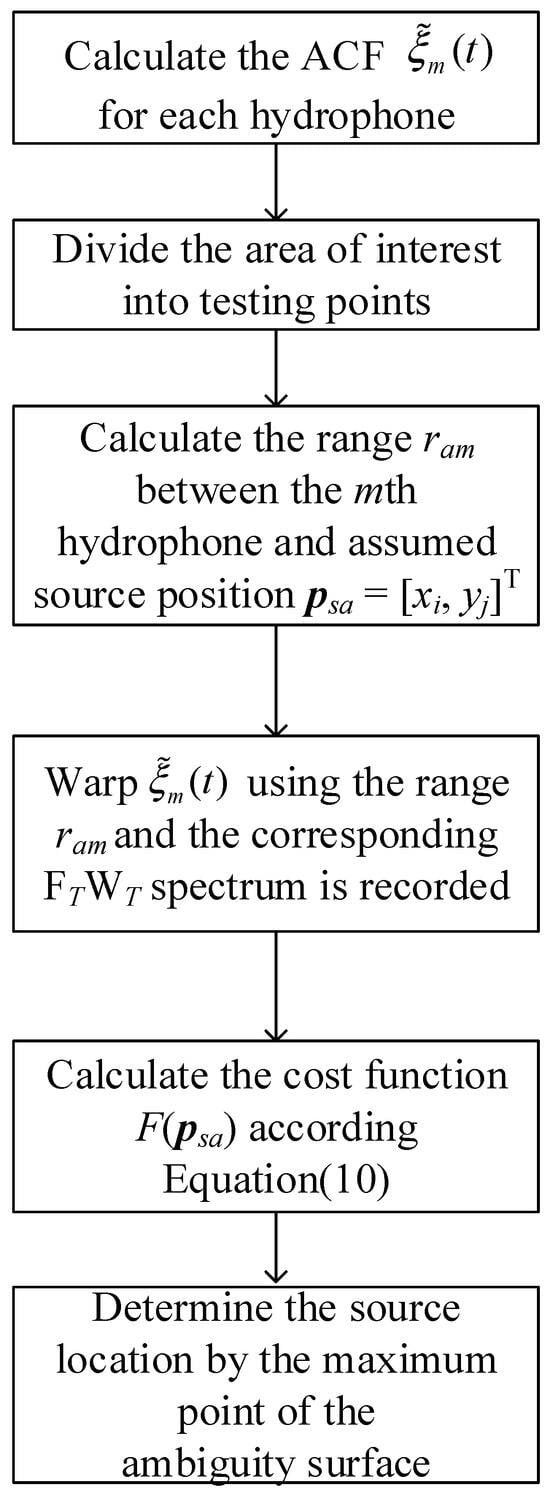
Figure 2.
The diagram the proposed method.
4. Simulation Demonstration
4.1. Effectiveness Verification
This section conducts numerical simulations in shallow water to validate the proposed method. A Pekeris waveguide, illustrated in Figure 3a, is considered in the simulation. The water depth is H = 100 m with a constant sound speed c = 1500 m/s and a constant density ρ1 = 1.0 g/cm3. The seabed is modeled as a soft half space. The density, sound speed, and attenuation coefficient are ρ2 = 1.0 g/cm3, c2 = 1600 m/s, α = 0.14 dB/λ, respectively.
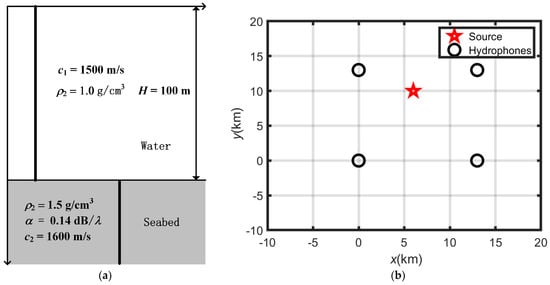
Figure 3.
Simulation Scene: (a) a Pekeris waveguide and (b) the top view of the source and distributed hydrophones.
The top view of the simulation scene is illustrated in Figure 3b. The source is located at ps = [6, 10]T km. The four hydrophones are at p1 = [0, 0]T km, p2 = [13, 0]T km, p3 = [0, 13]T km, and p4 = [13, 13]T km, respectively. Since the modal depth function varies with the receiving depth, the method requires all hydrophones to be deployed at the same depth. Both the source and the hydrophones are deployed at a depth of 20 m. The signal emitted by the source is modeled as a linear frequency modulation (LFM) signal. The duration and modulation band of the source signal are 3 s and [50, 150] Hz, respectively. The received field on the hydrophones is calculated by the KRAKEN normal mode code [25] with signal-to-noise (SNR) being set at 10 dB.
Figure 4 presents the normalized FTWT spectra from the distributed hydrophones for the scenario described in Figure 3b. Figure 4a,b correspond to the cases where the source location is correctly and incorrectly assumed, respectively. As can be seen, if the source location is correctly assumed (i.e., Figure 4a), the FTWT spectra for the different hydrophones shows the same shape. Otherwise, the consistency among the FTWT spectra will be disrupted as shown in Figure 4b. The results in Figure 4 convincingly demonstrate the feasibility of the proposed method.
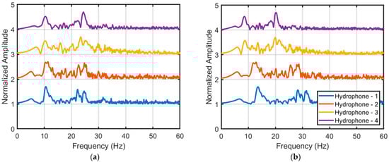
Figure 4.
Normalized FTWT spectra from distributed hydrophones. (a) With the correct source location; (b) with an incorrect source location, i.e., psa = [5, 5]T km.
Divide the area of interest (i.e., −10 km < x < 20 km, −10 km < y < 20 km) into grids with a step of 0.4 km and calculate the ambiguity surface using the algorithm shown in Figure 2. The sound speed used in the warping transform is ca = 1500 m/s. The obtained localization ambiguity surface is shown in Figure 5, wherein the cost function is normalized in decibels with a dynamic range of 10 dB. In Figure 5, the black asterisk donates the true source location, and the yellow circles represent the locations of the hydrophones. As can be seen, the ambiguity surface clearly peaks at the location of the source, demonstrating the effectiveness of the proposed method. In this simulation example, the localization result is [6.17, 10]T km with a localization error of 0.17 km. It is worth mentioning that the basic idea of the method is to mutually match the warped ACF obtained by distributed hydrophones, and the warping processing has nothing to do with the source depth. In other words, the method proposed in this paper can estimate the two-dimensional position of the sound source in the xoy plane when the source depth is unknown.
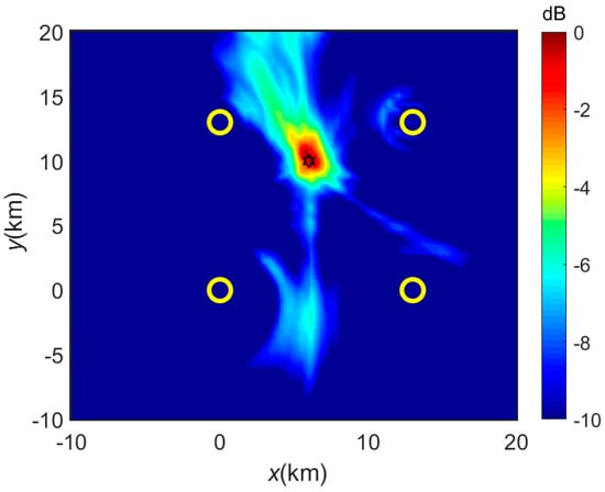
Figure 5.
Localization ambiguity surface. The black asterisk and yellow circles indicate the true source location and the location of the hydrophones, respectively. The black asterisk and yellow circles indicate the true source location and the location of the hydrophones, respectively.
The result of the warping transform is closely related to the assumed sound speed, i.e., a larger (or smaller) ca is equivalent to a smaller (or larger) assumed horizontal range rsam, thus resulting in a larger (or smaller) interference characteristic frequency (as shown in Equation (9)). Nevertheless, despite the influence of sound-speed mismatch on the result of the FTWT spectrum, the relative positions of the FTWT spectrum peak among sensors are independent of ca. Therefore, the proposed method still works as intended even if ca is mismatched with the true sound speed. The simulation results shown in Figure 6 confirm this speculation, where higher and lower sound speeds are used, respectively.
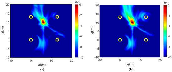
Figure 6.
Localization ambiguity surfaces with mismatched sound speed: (a) lower sound speed, i.e., ca = 1480 m/s; (b) higher sound speed, i.e., ca = 1520 m/s. The black asterisk and yellow circles indicate the true source location and the location of the hydrophones, respectively.
4.2. Performance Analysis
- Hydrophone Distribution
The hydrophone distribution is one of the important factors that affects the performance of the method. In this section, the localization ambiguity under different distributions of hydrophones will be analyzed through numerical simulations. According to the theoretical analysis in Section 3, the cost function reaches its maximum when the search grid point is identical to the source position (psa = ps). However, according to Equation (9), the cost function will also reach its maximum (equivalent to psa = ps) if the following equation holds:
Therefore, if there exists more than one point that satisfies Equation (13) in the area of interest, the ambiguity surface will exhibit more than one peak, and the localization result will become ambiguous. For example, if only two hydrophones are used, the points satisfying Equation (13) form a circle characterized by a radius of R = QL/|1 − Q2|, where Q is the distance ratio between the source and the two hydrophones, and L is the distance between these two hydrophones. Thus, the proposed method becomes invalid when only two hydrophones are used, as shown in Figure 7a. A fuzzy band emerges in the localization ambiguity surface and the true source location cannot be identified.
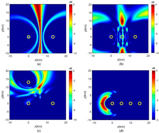
Figure 7.
The localization results under different hydrophones distributions: (a) two hydrophones; (b) three hydrophones with a colinear distribution; (c) three hydrophones with a non-colinear distribution; (d) four hydrophones with a colinear distribution and the source is also at this line. The black asterisk and yellow circles indicate the true source location and the location of the hydrophones, respectively. The black asterisk and yellow circles indicate the true source location and the location of the hydrophones, respectively.
When three hydrophones are deployed in a linear distribution, localization ambiguity arises, similar to the problem of port and starboard ambiguity for the DOA estimation using a linear array. The corresponding simulation result is shown in Figure 7b. As seen, a fuzzy source symmetric to the true counterpart appears. Changing the distribution of the hydrophones to a non-colinear arrangement allows unambiguous source localization, as shown in Figure 7c. Therefore, in practical applications, colinear distribution of hydrophones should be avoided. Finally, it is noteworthy that the colinear distribution can locate the source unambiguously when and only when the source is also on the same line, as shown in Figure 7d. But the performance of the method in this case is somewhat unsatisfying.
Define the area enclosed by the hydrophones as the detection area for the nonlinear distribution. The localization ambiguity of the proposed method can be numerically analyzed based on Equation (13). Specifically, one can count the number of the points (except ps) that satisfy Equation (13) in the detection area. The simulation results under different numbers of the hydrophones are shown in Figure 8, wherein the hydrophones are deployed through a regular M polygon. As seen with a M-polygon distribution, the proposed method can provide an unambiguous localization in the detection area.
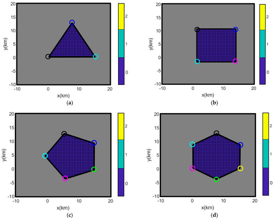
Figure 8.
The theoretical localization ambiguity of the method in the detection area under different number of hydrophones. (a–d) correspond to the cases where the number of the hydrophones is 3–6. The color bar indicates the number of the fuzzy peaks (i.e., the number of the points (except ps) that satisfy Equation (13)). The circles indicate the location of the hydrophones.
The above analysis leads to the conclusion that at least three sensors must be deployed to support the proposed method. In the colinear distribution scenario, a fuzzy peak symmetric to the true source will appear, except when the source is located on the line linking the hydrophones. When the hydrophones are deployed with a regular M polygon, there is no localization ambiguity in the detection area, i.e., the area enclosed by the hydrophones.
- Hydrophone Depth
The simulation environment in Section 4.1 is characterized by an isovelocity waveguide, where the reflected modes dominate the received field. However, in the non-isovelocity waveguide, the types of modes that dominate the received field depend on the depths of both the source and receiver. Different types of modes present different interference characteristics, which will affect the applicability of the proposed method. In this section, we take a classical thermocline waveguide as an example to analyze the effect of source and receiver depth on the performance of the proposed method.
The thermocline waveguide used in simulations is shown in Figure 9, which exhibits a classical downward-refracting sound speed profile (SSP) with a mixed layer depth down to 30 m. The sound speed reduces linearly from 1520 m/s to 1480 m/s as the depth changes from 30 m to 70 m. The sound speed, density, and the attenuation coefficient of the seabed are ρ2 = 1.0 g/cm3, c2 = 1600 m/s, and α = 0.14 dB/λ, respectively. Four different source–receiver configurations (a)–(d) are displayed in Figure 9. Assuming the source location is the same as the case in Figure 3b, the corresponding localization results are shown in Figure 10, where Figure 10a–d correspond to the four cases in Figure 9, one by one. The black asterisk and yellow circles indicate the true source location and the location of the hydrophones, respectively.
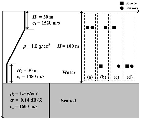
Figure 9.
The thermocline environment and different source-sensors depths configuration: (a) zs = 20 m, zr = 20 m, (b) zs = 70 m, zr = 20 m, (c) zs = 20 m, zr = 70 m, and (d) zs = 70 m, zr = 70 m.
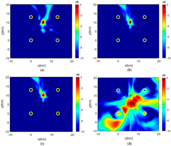
Figure 10.
The localization results with different source-sensors depths configurations under the thermocline waveguide: (a) zs = 20 m, zr = 20 m, (b) zs = 70 m, zr = 20 m, (c) zs = 20 m, zr = 70 m, and (d) zs = 70 m, zr = 70 m. The black asterisk and yellow circles indicate the true source location and the location of the hydrophones, respectively. Due to the general principle of reciprocity, scene (c) has the same result as (b).
As shown in Figure 10, the proposed method works as expected in the following two cases: (1) both the source and hydrophones are above the thermocline layer; (2) the source is above (or below) the thermocline layer while the hydrophones are below (or above) the thermocline layer. The proposed method becomes invalid if both the source and the hydrophones are below the thermocline layer.
Normal mode theory could be used to account for these simulation results. The modes distribution at 125 Hz for the waveguide in Figure 9 is depicted in Figure 11, which involves (a) the modes depth function and (b) the relationship between phase and group slowness. As can be seen in Figure 11, when both the source and hydrophones are deployed above the thermocline layer, or the source is above (or below) the thermocline layer while the hydrophones are below (or above) this layer, the received field is predominantly influenced by the higher order modes (i.e., n ≥ 3). When both the source and hydrophones are below the thermocline layer, the lower order (i.e., 1st and 2nd) modes dominate the field. The higher order modes correspond to the reflected modes while the lower order modes are the refracted modes. Following the conclusion in Ref. [26], the time warping function shown in Equation (7) is exclusively associated with the reflected modes, rendering it ineffective for the refracted modes. Therefore, the proposed method works well in the case that the reflected modes dominate the received field (i.e., the source and/or hydrophones are above the thermocline layer) and becomes invalid if the received field is dominated by the refracted modes (i.e., both the source and hydrophones are below the thermocline layer). As a result, it is recommended to deploy the hydrophones above the thermocline layer in the thermocline waveguide to improve the applicability of the proposed method.
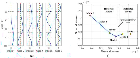
Figure 11.
The (a) modes depth function and (b) modes group (phase) slowness in the waveguide shown in Figure 9.
Similar simulations have been conducted to analyze the applicability of the proposed method under the positive/negative-gradient SSP waveguide. The results can be concluded as follows: (1) Modes generated under a negative-gradient SSP waveguide presents similar characteristics to those in the thermocline waveguide. Therefore, it is suggested to deploy the hydrophones near the sea surface to guarantee the effectiveness of the proposed method; (2) The depth function of the refracted mode generated under a positive-gradient SSP waveguide remains high amplitude near the sea surface while decaying exponentially near the seabed. Therefore, it is suggested to deploy the hydrophones near the seabed. All in all, in a non-isovelocity environment, hydrophones should be deployed at the depth with higher sound speed to guarantee the effectiveness of the proposed method.
5. Conclusions
In shallow water, the mode interference characteristic frequencies present an invariability property that is independent of the source–receiver geometry. Based on this phenomenon, a passive model-independent broadband source localization method utilizing distributed hydrophones is proposed in this paper. The basic idea of the proposed method is to mutually match the FTWT spectra from different hydrophones and determine the source location by verifying the invariability of the mode interference characteristic frequencies. Specifically, for an assumed source location, the time warping transform is firstly applied to the signal ACF to extract the interference characteristic frequencies for each hydrophone and then, a cost function is calculated to verify the consistency of the FTWT spectra from different hydrophones. The maximum point of the cost function indicates the location of the source.
Numerical simulations are conducted to demonstrate the performance of the method and the results can be concluded as follows: (1) the proposed method can locate the broadband source successfully in the classical Pekeris waveguide; (2) the method works as advertised in case that the reflected modes dominate the received field in the non-isovelocity environment (e.g., the thermocline waveguide). Thus, it is suggested to deploy the hydrophones at a depth with a higher sound speed to guarantee the effectiveness of the method; (3) the localization ambiguity can be avoided in the detection area (i.e., area enclosed by the hydrophones) when the hydrophones are distributed through a regular M polygon (M ≥ 3).
The proposed method theoretically circumvents the environmental mismatch problem by not relying on prior environment information. In addition, benefitting from exploiting the interference characteristics of the acoustic field, the proposed methods require neither the angle- nor time-synchronization information in its localization procedure. However, the drawbacks of this method are also obvious. Since the modal depth function varies with the receiving depth, the method in this paper requires all hydrophones to be deployed at the same depth. Meanwhile, the hydrophones should not be colinearly distributed.
In our work getting under the way, it is expected to analyze the localization ambiguity in detail with an arbitrary hydrophone distribution. Moreover, due to the fact that the method becomes invalid when the acoustic field is dominated by the refracted modes, how to exploit the interference characteristics of these refracted modes to locate the source is still an ongoing work.
Author Contributions
H.L.: Conceptualization, supervision, writing—review, funding acquisition. J.H.: Writing—editing, data curation. Z.X.: methodology, software, investigation, writing—original draft. K.Y.: Resources, project administration. J.Q.: Validation, funding acquisition. All authors have read and agreed to the published version of the manuscript.
Funding
This research was funded by the State Key Laboratory of Acoustics, Chinese Academy of Sciences (Grant No. SKLA202307), the National Natural Science Foundation of China (Grant No. 61901383 and No. 52231013), the Fundamental Research Funds for the Central Universities (Grant No. 3102021HHZY030011), and the Youth Innovation Promotion Association, Chinese Academy of Sciences (No. 2021023).
Data Availability Statement
Data will be made available on request.
Conflicts of Interest
The authors declare no conflicts of interest.
References
- Livingston, E. Effects of sound-speed mismatch in the lower water column on matched-field processing. J. Acoust. Soc. Am. 1992, 91, 2363–2364. [Google Scholar] [CrossRef]
- Jensen, F.B.; Kuperman, W.A.; Poter, M.B.; Schmidt, H. Computational Ocean Acoustics, 2nd ed.; Springer: New York, NY, USA, 2011. [Google Scholar]
- Cockrell, K.L.; Schmidt, H. Robust passive range estimation using the waveguide invariant. J. Acoust. Soc. Am. 2010, 127, 2780–2789. [Google Scholar] [CrossRef]
- Song, H.C.; Cho, C. Array invariant-based source localization in shallow water using a sparse vertical array. J. Acoust. Soc. Am. 2017, 141, 183–188. [Google Scholar] [CrossRef] [PubMed]
- Song, H.C.; Cho, C.; Byun, G.; Kim, J.S. Cascade of blind deconvolution and array invariant for robust source-range estimation. J. Acoust. Soc. Am. 2017, 141, 3270–3273. [Google Scholar] [CrossRef] [PubMed]
- Song, H.C.; Cho, C. The relation between the waveguide invariant and array invariant. J. Acoust. Soc. Am. 2015, 138, 899–903. [Google Scholar] [CrossRef] [PubMed]
- Qi, Y.-B.; Zhou, S.; Ren, Y.; Liu, J.-J.; Wang, D.-J.; Feng, X.-Q. Passive source range estimation with a single receiver in shallow water. Acta Acust. 2015, 40, 144–152. [Google Scholar]
- Zhou, S.; Qi, Y.; Ren, Y. Frequency invariability of acoustic field and passive source range estimation in shallow water. Sci. China-Phys. Mech. Astron. 2014, 57, 225–232. [Google Scholar] [CrossRef]
- Julien, B.; Aaron, T.M.; Susanna, B.B.; Katherine, K.; Michael, M.A. Range estimation of bowhead whale (Balaena mysticetus) calls in the Arctic using a single hydrophonea. J. Acoust. Soc. Am. 2014, 136, 145–155. [Google Scholar]
- Doğançay, K. Bearings-only target localization using total least squares. Signal Process. 2005, 85, 1695–1710. [Google Scholar] [CrossRef]
- Dogancay, K.; Ibal, G. Instrumental Variable Estimator for 3D Bearings-Only Emitter Localization. In Proceedings of the 2005 International Conference on Intelligent Sensors, Sensor Networks and Information Processing, Melbourne, Australia, 5–8 December 2005; pp. 63–68. [Google Scholar]
- Hawkes, M.; Nehorai, A. Wideband source localization using a distributed acoustic vector-sensor array. IEEE Trans. Signal Process. 2003, 51, 1479–1491. [Google Scholar] [CrossRef]
- Kaplan, L.M.; Le, Q.; Molnar, N. Maximum likelood methods for bearings-only target localization. In Proceedings of the 2001 IEEE International Conference on Acoustics, Speech, and Signal Processing (ICASSP), Salt Lake City, UT, USA, 7–11 May 2001; Volume 5, pp. 3001–3004. [Google Scholar]
- Kaplan, L.M.; Le, Q. On exploiting propagation delays for passive target localization using bearings-only measurements. J. Frankl. Inst. 2005, 342, 193–211. [Google Scholar] [CrossRef]
- Wang, Z.; Luo, J.; Zhang, X. A novel location-penalized maximum likelihood estimator for bearing-only target localization. IEEE Trans. Signal Process. 2012, 60, 6166–6181. [Google Scholar] [CrossRef]
- Luo, J.; Shao, X.; Peng, D.; Zhang, X. A Novel Subspace Approach for Bearing-Only Target Localization. IEEE Sens. J. 2019, 19, 8174–8182. [Google Scholar] [CrossRef]
- Chan, Y.T.; Ho, K.C. A simple and efficient estimator for hyperbolic location. IEEE Trans. Signal Process. 1994, 42, 1905–1915. [Google Scholar] [CrossRef]
- Foy, W.H. Position-Location Solutions by Taylor-Series Estimation. IEEE Trans. Aerosp. Electron. Syst. 1976, AES-12, 187–194. [Google Scholar] [CrossRef]
- Ho, K.C. Bias Reduction for an Explicit Solution of Source Localization Using TDOA. IEEE Trans. Signal Process. 2012, 60, 2101–2114. [Google Scholar] [CrossRef]
- Schau, H.; Robinson, A. Passive source localization employing intersecting spherical surfaces from time-of-arrival differences. IEEE Trans. Acoust. Speech Signal Process. 1987, 35, 1223–1225. [Google Scholar] [CrossRef]
- Laurinolli, M.H.; Hay, A.E. Localisation of right whale sounds in the workshop bay of fundy dataset by spectrogram cross-correlation and hyperbolic fixing. Can. Acoust. 2004, 32, 132–136. [Google Scholar]
- Desharnais, F.; Côté, M.; Calnan, C.J.; Ebbeson, G.R.; Thomson, D.J.; Collison, N.E.; Gillard, C.A. Right whale localisation using a downhill simplex inversion scheme. Can. Acoust. 2004, 32, 137–145. [Google Scholar]
- Bonnel, J.; Touze, G.L.; Nicolas, B.; Mars, J.I.; Gervaise, C. Automatic and passive whale localization in shallow water using gunshots. In Proceedings of the OCEANS 2008, Quebec City, QC, Canada, 15–18 September 2008; pp. 1–6. [Google Scholar]
- Gervaise, C.; Vallez, S.; Stephan, Y.; Simard, Y. Robust 2D localization of low-frequency calls in shallow waters using modal propagation modelling. Can. Acoust. 2008, 36, 153–159. [Google Scholar]
- Porter, M.B. The KRAKEN Normal Mode Program; Technical Report; Naval Research Laboratory: Washington, DC, USA, 1992. [Google Scholar]
- Qi, Y.; Zhou, S.; Zhang, R. Warping transform of the refractive normal mode in a shallow water waveguide. Acta Phys. Sin. 2016, 65, 134301. [Google Scholar] [CrossRef]
Disclaimer/Publisher’s Note: The statements, opinions and data contained in all publications are solely those of the individual author(s) and contributor(s) and not of MDPI and/or the editor(s). MDPI and/or the editor(s) disclaim responsibility for any injury to people or property resulting from any ideas, methods, instructions or products referred to in the content. |
© 2024 by the authors. Licensee MDPI, Basel, Switzerland. This article is an open access article distributed under the terms and conditions of the Creative Commons Attribution (CC BY) license (https://creativecommons.org/licenses/by/4.0/).