Improvements in the Estimation of Air Temperature with Empirical Models on Livingston and Deception Islands in Maritime Antarctica (2000–2016) Using C6 MODIS LST

Abstract

Temperature analysis is of special interest in polar areas because temperature is an essential variable in the energy exchange between the Earth’s surface and atmosphere. Although land surface temperature (LST) obtained using satellites and air temperature (T_a) have different physical meanings and are measured with different techniques, LST has often been successfully employed to estimate T_a. For this reason, in this work, we estimated T_a from LST MODIS collection 6 (C6) and used other predictor variables. Daily mean T_a was calculated from Spanish State Meteorological Agency (AEMET) stations data on the Livingston and Deception Islands, and from the PERMASNOW project stations on Livingston Island; both islands being part of the South Shetland Islands (SSI) archipelago. In relation to our previous work carried out in the study area with collection 5 (C5) data, we obtained higher R² values (R²_CV = 0.8, in the unique model with Terra daytime data) and lower errors (RMSE_CV = 2.2 °C, MAE_CV = 1.6 °C). We corroborated significant improvements in MODIS C6 LST data. We analyzed emissivity as a possible factor of discrepancies between C5 and C6, but we did not find conclusive results, therefore we could not affirm that emissivity is the factor that causes differences between one collection and another. The results obtained with the applied filters indicated that MODIS data can be used to study T_a in the area, as these filters contribute to the reduction of uncertainties in the modeling of T_a from satellites.

1. Introduction

Temperature, defined as a physical quantity that characterizes the average energy of random molecular motion within a substance [1,2], is an essential variable in the energy exchange between the Earth’s surface and the atmosphere [3,4,5,6,7,8]. In meteorology, air temperature at various heights and the temperature of the ground surface can be measured, among others [1], the latter being the one that corresponds to land surface temperature (LST) obtained from satellites.

Air temperature (T_a) can also influence the behavior of the active permafrost layer, as described for James Ross Island (JRI)—one of the largest permafrost regions in the northeastern Antarctic Peninsula (PA)—by Hrbáček et al. [9], who found a significant effect of T_a on the thermal regime of the soil, especially in the absence of snow and during the advection of warm air masses that cause important gradients in T_a during winter. In addition, major changes in temperature could lead to changes in the snowpack on the Antarctic ice sheet, which would have both immediate and long-term impacts on the global mean sea level [10]. Therefore, T_a constitutes an essential parameter in a wide range of environmental applications, such as hydrology and climate change studies [11]. Surface temperature, for its part, is the primary climatic factor that governs the existence, spatial distribution and thermal regime of permafrost which is a major component of the terrestrial cryosphere [12]. In summary, both Ta and LST constitute essential factors for permafrost, which is determined by the climate and the geothermal gradient [13].

T_a and LST generally present a similar behavior that can be considered as a sinusoidal oscillation with a period of one year. It is also known that ground temperature can delay T_a variations [14], therefore it could be considered that this energy exchange can favor the correlation between T_a and LST. However, it must be taken into account that T_a and LST are two different variables, and the correlation between them could vary throughout the year because in the cold season the snow acts as an insulating layer [15]. In addition, it has been described that the correlation also depends on land cover and sky conditions [16,17], as well as elevation changes [18], latitude and solar radiation. On the other hand, land and air have different thermal capacities [19,20] and T_a and LST have different physical meanings and are measured with different techniques: for example, in the case of the Moderate Resolution Imaging Spectroradiometer (MODIS), LST data indicate the land surface temperature in an area of 1 km², while, in this work, T_a refers to the temperature measured 2 m above the ground surface. Also, unlike T_a, LST provides direct information on long-wave radiation from the Earth’s surface [19].

However, its different nature has not prevented LST from becoming an important alternative to overcome the lack of T_a data, generally only obtained at certain points with very limited area coverage [18]. Likewise, LST has been used to validate in situ data on surface air temperature (T_s) [21]. Furthermore, as indicated by Sobrino et al. [22], it is known that there is a correspondence between LST and T_a, in general terms—not only with MODIS sensor data—as has been shown for local studies, among others, by the works of Jin and Dickinson [19,23], Prihodko and Goward [24] and Urban et al. [25].

The possibility of having LST measurements from satellites has favored the development of studies for the estimation of T_a. The high temporal resolution of MODIS has made it possible to widely develop studies on the temperature of the polar regions [6]. The utility of applying statistical methods to MODIS sensor data, due to its high temporal resolution, is evident in the numerous works that have estimated T_a with MODIS LST data in various study areas including Portugal [11] and the United States [26]. Also, statistical methods combined with the Temperature-Vegetation Index (TVX) have been used on different sites in Africa [27]. The above examples highlight the variety of ecosystems that are represented in these studies.

In Antarctica, there have been several works that estimated T_a from MODIS LST data with statistical methods. Also Meyer et al. (2016) [28] estimated T_a values using MODIS data and data from 32 weather stations in Antarctica, adding to LST other predictor variables to three machine learning algorithms: Random Forest (RF), Gradient boosting (GBM) and cubist. In addition, MODIS LST has been used to model the near-surface permafrost temperature [29] in all ice-free areas in Antarctica and on Antarctic islands, using reanalysis data. Intercomparison studies between MODIS LST and T_a in situ data have also been carried out; for example, Wang et al. [30], based on the monthly average values and measurements of T_a at 1 m and 2 m, in stations in Eastern Antarctica.

Analysis of numerous authors who have studied temperature variability [31,32,33,34,35,36,37,38,39,40,41,42,43,44] demonstrates the complexity of Antarctic climatology, on both a spatial and temporal scale, observed on and around the Antarctic Peninsula (AP), it is essential to continue monitoring it with both in situ T_a and satellite LST data. But the in situ T_a data, although continuous and precise, are spatially sparse, so the LST could help, after comparing with the T_a, to extend the spatial coverage of these data, in spite of the known drastic reduction in LST data due to the frequent cloudiness in the regions of the Antarctic. 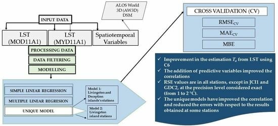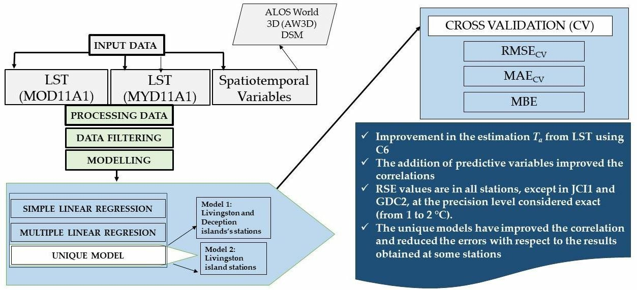On the other hand, the estimation of T_a from LST will be more precise as the LST data are more precise, so the improvement of the LST data is essential, both with new methods and new sensors. 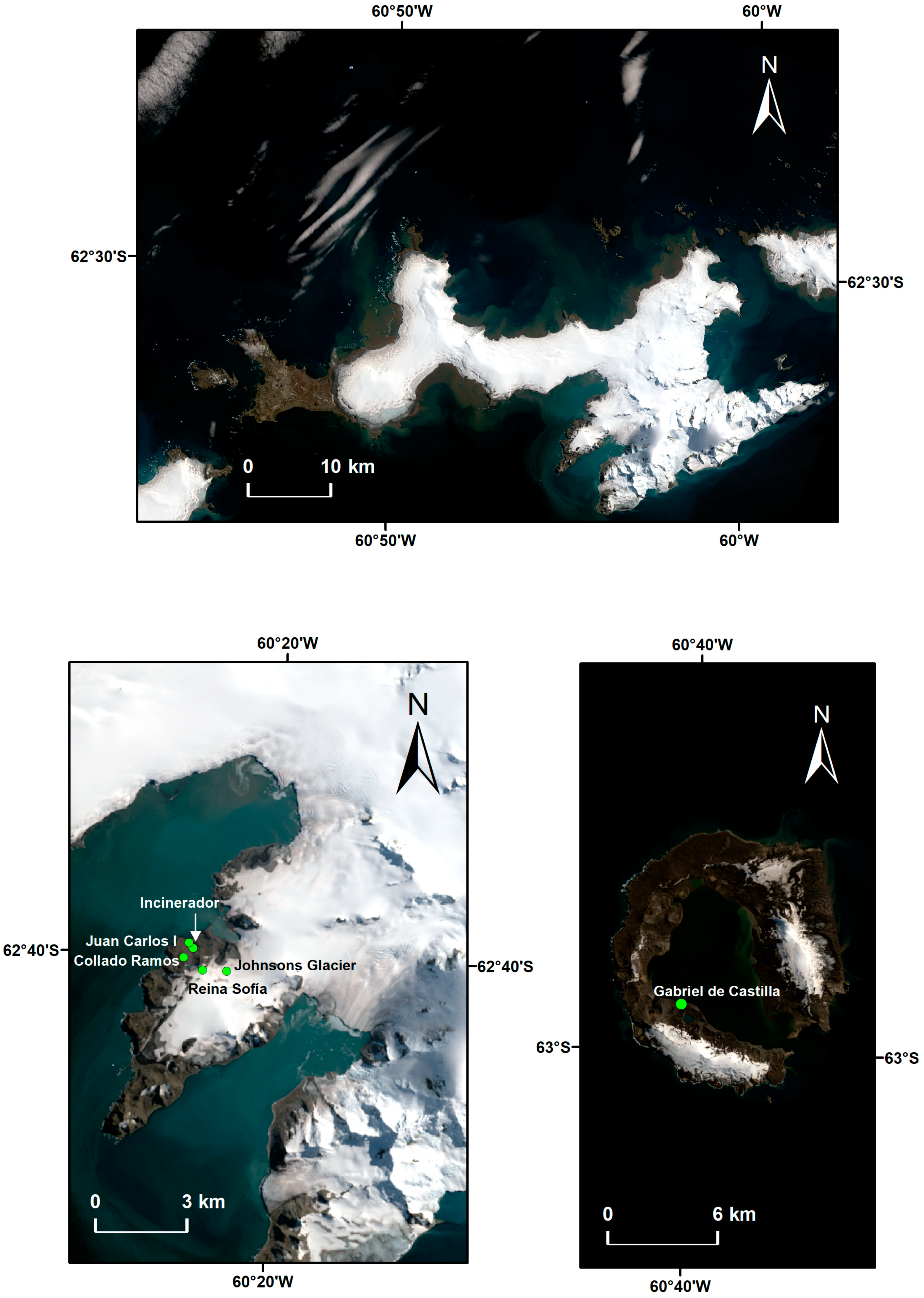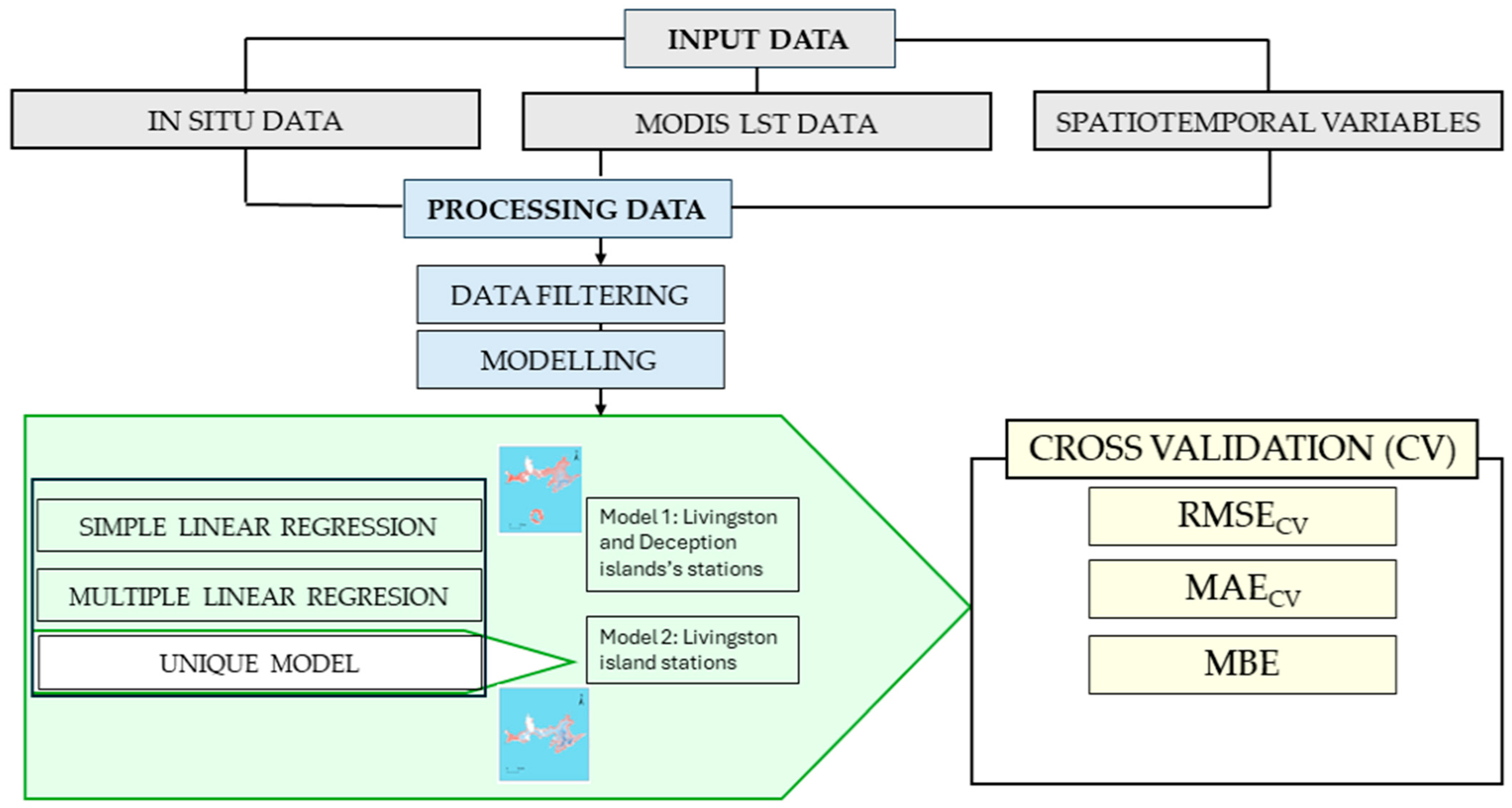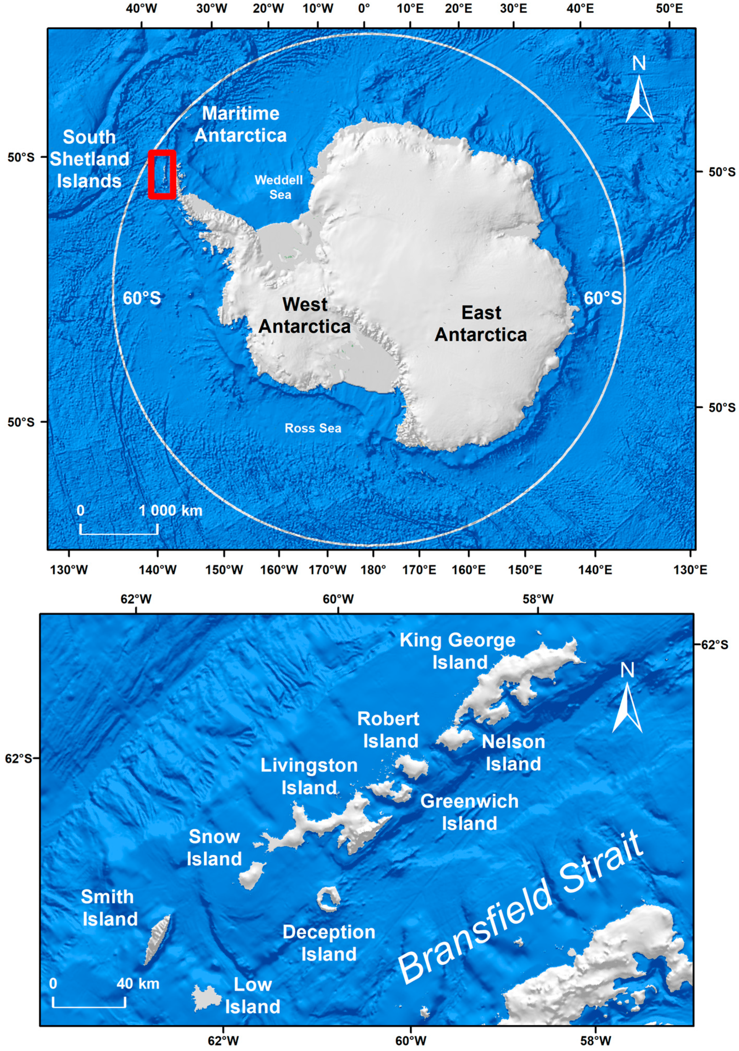In this scenario, the aim of this work is to estimate T_a from daytime and nighttime LST data at Maritime Antarctica sites in the South Shetland Archipelago using empirical models, based on the addition of spatiotemporal variables to LST. The need to use satellites and sensors to estimate in situ data in polar areas is well known, given the impossibility of installing and maintaining a dense network of stations in these areas. To date, the estimation of T_a from MODIS 6 (C6) collection data has not been performed on Livingston Island. In the case of Deception Island, T_a has not been estimated with any MODIS collection so far. In addition, this work analyses the emissivity, taking into account that in C6 important changes were introduced with respect to collection 5 (C5), especially in the emissivity adjustment.

Following the Introduction (Section 1), in Materials and Methods (Section 2) we describe the study area, MODIS and in situ data, as well as the digital terrain model data and methodology used to compare T_a with LST. The sections on Results, Discussion and Conclusions are provided in Section 3, Section 4 and Section 5, respectively.

2. Materials and Methods

Figure 1 shows the analytical framework for estimating T_a from LST.

2.1. Study Area

This work focuses on the Livingston and Deception Islands, both in the South Shetland Island (SSI) archipelago (Figure 2), which occupies an area of 3687 km² and is in Maritime Antarctica, approximately 120 km from the AP, separated from South America by the Drake Passage and from the Antarctic continent by the Bransfield Strait. Livingston Island (Figure 3), the second largest in the SSI, with an area of 974 km², is located 110 km northwest of Cape Roquemaurel, in Antarctica; 830 km south-southeast of Cape Horn and 820 km southeast of the Diego Ramírez Islands, both in Chile, and 3000 km from the South Pole; 90% of its surface is covered with ice all year round [45]. The Juan Carlos I (JCI) Spanish Antarctic base is located on this island. Deception Island (Figure 3), much smaller than Livingston Island and of volcanic origin, has an average diameter of 15 km, and it is 110 km from AP. The Gabriel de Castilla (GDC) Spanish Antarctic base is located on it. The climatology of the SSI and the AP, as well as the Antarctic continent in general, is ideal for studying atmospheric turbulence and energy exchanges, radiative fluxes, snow drift, precipitation and accumulation mechanisms, among other phenomena that would have an influence on the global climate, therefore these studies would facilitate forecasting tasks [46]. These characteristics, together with the fact that the permafrost in the SSI presents a very complex distribution [47], make the archipelago an important center for monitoring meteorological variables, including T_a.

2.2. MODIS LST

The MODIS sensor is onboard the Terra and Aqua satellites, which have sun-synchronous orbits, with almost polar inclination [48,49], which allows for two images per day for each satellite to be obtained [50]. The MOD11A1 (Terra Land Surface Temperature and Emissivity Daily Global 1 km) and MYD11A1 (Aqua Land Surface Temperature and Emissivity Daily Global 1 km) products provide daytime and nighttime Terra and Aqua LST data, respectively. They were obtained with the Generalized Split Window (GSW) algorithm, from MODIS bands 31 and 32 data (10.78–11.28 μm and 11.77–12.27 μm, respectively) [51]. According to these authors, GSW allows for greater precision and, furthermore, is less affected by the uncertainty associated with the emissivity and optical properties of the atmosphere. In GSW, LST is initially obtained using the following equation:

$$LST=b_0+\left(b_1+b_2\frac{1-\epsilon }{\epsilon }+b_3\frac{∆\epsilon }{{\epsilon }^2}\right)\frac{T_i+T_j}{2}+\left(b_4+b_5\frac{1-\epsilon }{\epsilon }+b_6\frac{∆\epsilon }{{\epsilon }^2}\right)\frac{T_i-T_j}{2}$$

(1)

where ε and ∆ε are the mean and difference of emissivity values in MODIS bands 31 and 32, i is band 31, j is band 32 and $b_k$ (k = 0–6) are coefficients that depend on the viewing zenith angle, surface air temperature and atmospheric column water vapor, and were derived from regression analysis of radiative transfer simulation data for LST values varying from T_a – 16 K to T_a + 16 K [51,52].

Many improvements were introduced in Collection 6 (C6), such as the removal of data contaminated by clouds at levels 2 and 3 [6]. Furthermore, for example, in C6, in MOD11A1, LST values in all grids are from MODIS observations obtained under clear-sky conditions [53]. It is known that, in remote sensing, LST can only be measured in clear sky conditions, since the presence of clouds introduces biases. However, overcorrection, especially from statistical methods, could also introduce errors. Specifically, in the GSW algorithm, the most notable changes in C6 are related to the separation of the coefficients to recover day and night LST over bare soil surfaces in latitudes from −38° to 49.5°, the emissivity differences in MODIS bands 31 and 32 over bare soil surfaces were adjusted and incorporated the quadratic difference between brightness temperatures in bands 31 and 32 into the equation. In this way, in C6, LST is recovered using the following equation [52]:

$$LST=b_0+\left(b_1+b_2\frac{1-\epsilon }{\epsilon }+b_3\frac{∆\epsilon }{{\epsilon }^2}\right)\frac{T_i+T_j}{2}+\left(b_4+b_5\frac{1-\epsilon }{\epsilon }+b_6\frac{∆\epsilon }{{\epsilon }^2}\right)\frac{T_i-T_j}{2}+b_7{\left(T_i-T_j\right)}^2$$

(2)

where a quadratic term has been added to Equation (1) with the difference between the brightness temperatures in bands 31 and 32 depending on the viewing angle [52]. The MODIS data used in this work were obtained through the Google Earth Engine (GEE) platform [54].

LST Data Quality Filters

MODIS LST product quality bits indicate some of the errors that may be present, including cloud mask failures and emissivity errors. For this study, only the highest quality data (QC = 00 in all bits) were selected. In addition, we filtered the data using the albedo products. Considering that sometimes MODIS cloud mask fails and that, in addition, the repercussion of these errors can increase in LST products, due to their lower spatial resolution compared to the albedo MODIS products (1000 m and 500 m, respectively), MOD11A1 and MYD11A1 data were filtered taking into account the information of the Snow_Albedo_Daily_Tile layer of the MOD10A1 and MYD10A1 products, respectively, and those corresponding to “clouds” were eliminated.

Once the previously explained filters were applied, some outliers were still observed. It is known that these outliers can be caused by cloud pollution [11] and must be removed to obtain robust LST validation statistics [55]. Likewise, previous studies indicate that this problem can be solved through statistical methods [56,57]. Therefore, those values considered outliers were eliminated here; that is, those that were outside the range between the lower (C_l) and upper (C_u) dataset caps, calculated using Equations (3) and (4), respectively,

$$C_l=Q_1-1.5(Q_3-Q_1)$$

(3)

$$C_u=Q_3+1.5\left(Q_3-Q_1\right)$$

(4)

where Q₁ and Q₃ are the first and third quartile of the data. This method has been used to detect outliers in MODIS LST studies [18,58,59,60].

2.3. In Situ Data

T_a data, at a height of ~2 m above ground, were taken from the AEMET stations Juan Carlos I (JCI) and Johnsons Glacier (JG) on Livingston Island and Gabriel de Castilla (GDC) on Deception Island, and from the PERMASNOW project stations Incinerador (INC), Reina Sofía (SOF) and Collado Ramos (CR) on Livingston Island [61,62]. T_a data are obtained every 10 min in JCI and GDC throughout the year and in JG from December to February, whereas, during the rest of the year, they are obtained every half hour. In all cases, the instruments have a precision of ±0.1 °C [63,64]. Daily mean T_a was only obtained at each weather station if daily data were complete (n = 144 for 10-min data and n = 48 for half-hourly data).

Table 1. Study period taken into account for the stations.

Station	Latitude	Longitude	Operation Dates
JCI1	62°39′47″S	60°23′16″W	1 January 2000–30 December 2009
JCI2	62°39′48″S	60°23′19″W	31 December 2009–10 April 2020
JG	62°40′16″S	60°21′51″W	1 December 2006–24 January 2015
GDC2	62°58′38″S	60°40′33″W	12 February 2007–10 April 2020
INC2	62°39′53″S	60°23′08″W	23 January 2006–9 February 2016
SOF	62°40′16″S	60°22′46″W	23 February 2002–20 January 2015
CR	62°40′03″S	60°23′32″W	2 February 2006–9 February 2016

indicates the study period taken for each station. At INC and GDC stations, only data corresponding to the current location (INC2 and GDC2, respectively) were used, given the lack of MODIS quality data in GDC1 and instrument failures in INC1. Data were filtered following Recondo et al. [64].

2.4. Digital Terrain Model Data

The topographic variables included in the model to estimate T_a were obtained from the DEM ALOS World 3D (AW3D), published by the Japan Aerospace Exploration Agency, Tokyo, Japan (JAXA) in 2016, which was generated using images from the Panchromatic Remote-sensing Instrument for Stereo Mapping (PRISM) sensor, which is on board the Advanced Land Observing Satellite (ALOS) [65]. The dataset used has a spatial resolution of 30 m (AW3D30) [65].

2.5. T_a Estimation

To estimate T_a from LST, both variables were compared, using the daily mean T_a data and MOD11A1 and MYD11A1 daytime and nighttime data. To quantify the goodness of fit, the following statistics were used: R² and residual standard error (RSE).

$$RSE=\sqrt{\frac{\sum {(y-\widehat{y})}^2}{v}}$$

(5)

where $\widehat{y}$ is the $y$ value predicted by the model and $v$ are the degrees of freedom, calculated as the total number of observations minus the number of parameters. In addition to simple linear regressions, to estimate T_a, multiple linear regressions were used for each station, in which variables from a harmonic model were included (Equation (6)), following Recondo et al. [64]:

$$T_a=c_1+c_{2}LST+c_{3}t+c_4\sin 2\pi t+c_5\cos 2\pi t$$

(6)

where $c_i$ are constants, LST and T_a are in °C and t is time in decimal year units.

Then, we built a unique model including T_a from all the stations along with topographic variables and other spatiotemporal variables (distance to the coast, latitude, longitude and LST observation time), just as we did in a previous work [64]. Previous studies in other regions around the world have used spatiotemporal variables in the estimation of meteorological variables from MODIS data [11,66,67]. The structure of our unique model is based on Equation (7):

$$T_a=c_1+c_{2}LST+c_{3}t+c_4\sin 2\pi t+c_5\cos 2\pi t+c_{6}c+c_{7}s+c_{8}h+c_{9}r+c_{10}a+c_{11}H$$

(7)

where c_i are constants, LST and T_a are in °C; t is the time in decimal year units; c is the curvature in m⁻¹; $s$ is the slope in degrees; h is the height in m; r is the roughness, calculated as the variance of the slope [68], dimensionless; $a$ is the aspect in radians and H is LST observation time. Only statistically significant variables (p value ≤ 0.05) were included in the final models obtained.

As a matter of fact, two unique models were built: one for all the stations including GDC and another only for the Livingston Island stations. This separation is due to the different characteristics of Deception Island, where in the summer most of the surface is bare soil, unlike Livingston Island, where up to 90% usually remains covered with snow/ice during that period [45,69]. On the other hand, although slight, there are also some differences in terms of ground cover with mosses/lichens on both islands: while on Deception Island, in the area near GDC, the presence of organic matter is negligible [70], on Livingston the populations of D. antarctica and C. quitensis have been reported, although the rate of demographic expansion is not very rapid [71].

Finally, the applied models were evaluated using the leave-one-out cross-validation method (CV), based on the R²_CV, MAE_CV, RMSE_CV and Bias statistics.

$$MAE=\frac{\sum \left|y_{observed}-y_{estimated}\right|}{n}$$

(8)

$$RMSE=\sqrt{\frac{\sum {(y_{observed}-y_{estimated})}^2}{n}}$$

(9)

$$Bias=\frac{\sum (y_{observed}-y_{estimated})}{n}$$

(10)

where $y_{observed}$ are the observed data, $y_{estimated}$ are the estimated data by a given model and n is the total amount of data.

3. Results

3.1. Simple Linear Regression T_a-LST

Table 2. Results for simple linear regression (daily mean T_a-LST).

Station	MODIS Data	n	R2	RSE (°C)
JCI1	Terra-Day	54	0.68	2.58
	Terra-Night	30	0.56	2.88
	Aqua-Day	56	0.78	2.52
	Aqua-Night	21	0.69	3.31
JCI2	Terra-Day	74	0.78	1.76
	Terra-Night	29	0.60	2.71
	Aqua-Day	65	0.78	1.86
	Aqua-Night	27	0.71	2.93
JG	Terra-Day	23	0.64	1.53
	Terra-Night	22	0.29	1.38
	Aqua-Day	66	0.62	2.25
	Aqua-Night	Not applicable
INC2	Terra-Day	83	0.73	1.96
	Terra-Night	48	0.63	2.24
	Aqua-Day	87	0.73	2.46
	Aqua-Night	45	0.62	2.82
SOF	Terra-Day	78	0.71	1.61
	Terra-Night	83	0.54	2.20
	Aqua-Day	190	0.62	2.61
	Aqua-Night	44	0.44	3.37
CR	Terra-Day	56	0.77	2.32
	Terra-Night	46	0.64	2.36
	Aqua-Day	75	0.77	2.27
	Aqua-Night	33	0.62	3.43
GDC2	Terra-Day	58	0.79	2.43
	Terra-Night	31	0.56	4.29
	Aqua-Day	66	0.76	2.29
	Aqua-Night	35	0.37	3.35

shows the results for the simple linear regression from MODIS daily daytime and nighttime C6 values and in situ data for all stations. In our case, a better fit is always achieved with daytime data (R² average = 0.73) than with nighttime data (R² average = 0.56). If we analyze the spatial variation of the correlation, we see that, of all the stations, the best behavior in terms of R² is obtained in GDC2 (R² = 0.79, with Terra daytime data), followed by JCI2 (R² = 0.78, with Terra and Aqua daytime data), JCI1 (R² = 0.78, with Aqua daytime data) and CR (R² = 0.77, with Terra and Aqua daytime data).

In summary, all stations show a good fit with the daytime data, with an R² = 0.62–0.79. On the other hand, the mean RSE for daytime data is 2.18 °C, with only two stations showing errors greater than 2.5 °C (SOF, MYD11A1, RSE = 2.61 °C and JCI1, MOD11A1, RSE = 2.58 °C). The range of RSE is between 1.53 and 2.58 °C. Likewise, although R² average values of the daytime data from Terra and Aqua are similar (0.73 and 0.72, respectively), Terra data present, with an average of 2.03 °C, lower RSE values than those from Aqua, the average RSE of which increases to 2.32 °C. For this reason, we can affirm that the daytime data from Terra present a better agreement with in situ data.

3.2. Models of T_a Based in Multiple Linear Regressions

In relation to the simple linear regression analyzed in the previous section, our results, shown in

Table 3. Results of the multiple linear regression for the estimation of T_a for each station, following Equation (6).

Station	MODIS Data	n	R2	RSE (°C)	c1	c2 (LST)	c3 (t)	c4 (sin)	c5 (cos)
JCI1	Terra-Day	54	0.71	2.10	659 ± 287	0.56 ± 0.06	−0.33 ± 0.14	0	0
	Terra-Night	30	0.56	2.88	1.31 ± 1.66	0.64 ± 0.13	0	0	0
	Aqua-Day	56	0.78	2.52	−1.53 ± 0.39	0.61 ± 0.04	0	0	0
	Aqua-Night	21	0.69	3.31	4.38 ± 2.20	0.98 ± 0.16	0	0	0
JCI2	Terra-Day	74	0.80	1.48	0.5 ± 0.3	0.69 ± 0.05	0	0	−1.5 ± 0.5
	Terra-Night	29	0.60	2.71	1.30 ± 1.07	0.59 ± 0.09	0	0	0
	Aqua-Day	65	0.78	1.86	−0.57 ± 0.27	0.51 ± 0.03	0	0	0
	Aqua-Night	27	0.71	2.93	2.39 ± 1.30	0.75 ± 0.10	0	0	0
JG	Terra-Day	23	0.64	1.53	−1.15 ± 0.39	0.39 ± 0.05	0	0	0
	Terra-Night	22	0.53	1.66	0.5 ± 1.3	0.29 ± 0.12	0	0	3.0 ± 1.2
	Aqua-Day	66	0.67	2.21	−2.4 ± 0.5	0.40 ± 0.04	0	1.5 ± 0.5	0
	Aqua-Night	Not applicable
INC2	Terra-Day	83	0.77	1.34	−537 ± 126	0.57 ± 0.03	0.27 ± 0.06	0	0
	Terra-Night	48	0.63	2.24	1.30 ± 0.82	0.64 ± 0.06	0	0	0
	Aqua-Day	87	0.76	2.25	−611 ± 178	0.54 ± 0.03	0.30 ± 0.09	0	0
	Aqua-Night	45	0.66	2.45	−741 ± 273	0.81 ± 0.09	0.37 ± 0.14	0	0
SOF	Terra-Day	78	0.75	1.71	−392 ± 127	−0.55 ± 0.04	0.19 ± 0.06	0	0
	Terra-Night	83	0.54	2.20	−0.68 ± 0.72	0.61 ± 0.06	0	0	0
	Aqua-Day	190	0.65	2.78	−231 ± 115	0.60 ± 0.05	0.11 ± 0.006	0.7 ± 0.3	1.4 ± 0.6
	Aqua-Night	44	0.56	2.77	−4 ± 2	0.57 ± 0.12	0	−5.1 ± 1.9	0
CR	Terra-Day	56	0.81	1.75	−590 ± 163	0.57 ± 0.04	0.29 ± 0.08	0	0
	Terra-Night	46	0.64	2.36	0.78 ± 1.01	0.63 ± 0.07	0	0	0
	Aqua-Day	75	0.81	2.07	−498 ± 178	0.67 ± 0.06	0.25 ± 0.09	0	−1.8 ± 0.7
	Aqua-Night	33	0.75	2.76	−1245 ± 322	0.74 ± 0.09	0.6 ± 0.2	0	0
GDC2	Terra-Day	58	0.82	2.30	1.0 ± 0.4	0.84 ± 0.08	0	0	−2.3 ± 0.8
	Terra-Night	31	0.56	4.29	5.39 ± 1.96	0.89 ± 0.16	0	0	0
	Aqua-Day	66	0.76	2.29	−0.22 ± 0.47	0.60 ± 0.04	0	0	0
	Aqua-Night	35	0.37	3.35	0.62 ± 1.74	0.56 ± 0.15	0	0	0

, improve, in general, with the addition of new variables.

In all cases in which at least one of the three added variables was significant, the R² values are higher. As in simple regression, here, too, better results were obtained with daytime data (R² average = 0.75) than with nighttime data (R² average = 0.60), and specifically with Terra daytime data (R² average = 0.76).

On the other hand, when applying the model obtained with Equation (6), RSE values obtained are in the range of 1.34 to 3.35 °C, except in GDC2, with the nocturnal data from Terra, where they reach 4.29 °C. In fact, if we exclude JCI1 and GDC2, at least with Terra daytime data at all stations, the RSE values are at the precision level considered exact (1 to 2 °C) according to Benali et al. [11]. Subsequently, spatiotemporal variables were added to the model of Equation (6), with the purpose of obtaining two unique models, both from Equation (7), the first of them only with Livingston Island stations (

Table 4. Unique model to estimate T_a from LST, excluding GDC, following Equation (7).

MODIS Data	n	R2	RSE (°C)	c1 (°C)	c2 (LST)	c3 (t)	c4 (sin)	c5 (cos)	c6 (c)	c7 (s)	c8 (h)	c9 (r)	c10 (a)	c11 (H)
Terra-Day	368	0.76	1.56	−184 ± 53	0.67 ± 0.03	0.10 ± 0.03	0	−1.3 ± 0.3	0	20 ± 9	−0.03 ± 0.01	572 ± 271	−0.7 ± 0.3	−0.7 ± 0.2
Terra-Night	258	0.61	2.30	2.1 ± 0.5	0.59 ± 0.03	0	0	1.7 ± 0.5	156 ± 34	−3.58 ± 1.09	0	0	0	0
Aqua-Day	539	0.74	2.34	−197 ± 63	0.59 ± 0.03	0.10 ± 0.03	0.39 ± 0.17	−1.1 ± 0.3	329 ± 85	−7 ± 2	0.02 ± 0.01	0	−0.36 ± 0.16	0
Aqua-Night	191	0.69	2.98	−442 ± 136	0.73 ± 0.05	0.22 ± 0.07	−3.8 ± 0.9	0	0	0	0	0	0	−0.07 ± 0.03

), and the second including GDC (

Table 5. Unique model to estimate T_a from LST, including GDC, following Equation (7).

MODIS Data	n	R2	RSE (°C)	c1 (°C)	c2 (LST)	c3 (t)	c4 (sin)	c5 (cos)	c6 (c)	c7 (s)	c8 (h)	c9 (r)	c10 (a)	c11 (H)
Terra-Day	426	0.76	1.71	−143 ± 50	0.69 ± 0.03	0.07 ± 0.02	0	−1.3 ± 0.2	141 ± 24	−2.8 ± 0.7	0	0	0	−0.60 ± 0.19
Terra-Night	289	0.59	2.48	2.4 ± 0.5	0.61 ± 0.03	0	0	1.6 ± 0.6	167 ± 34	−3.88 ± 1.14	0	0	0	0
Aqua-Day	560	0.74	2.36	−182 ± 58	0.59 ± 0.03	0.09 ± 0.03	0.53 ± 0.16	−1.1 ± 0.03	142 ± 30	0	0	−78 ± 33	0	0
Aqua-Night	226	0.65	2.88	−434 ± 113	0.72 ± 0.04	0.22 ± 0.06	0	4.3 ± 0.8	0	0	0	0	0	−0.06 ± 0.02

). In both cases, the following significant explanatory variables were added to the model: curvature (c₆, c), slope (c₇, s), height (c₈, h), roughness (c₉, r), aspect (c₁₀, a) and time of LST observation (c₁₁, H). Obtaining two unique models allows for mapping the behavior of the T_a in the study area.

In the case of the unique model that excludes GDC2, if we compare its results with those obtained after individually applying the model to each of the stations, we can see increases in R² values with respect to the daytime and nighttime Terra data obtained at JG station. Likewise, the single model shows lower RSE values than the stations in several cases, for example, if compared to JCI1, the model error decreases for all MODIS LST data, presenting values below 2.5 °C, except for the Aqua-night data, where it reaches a value of 2.98 °C. Regarding the unique model that includes Deception Island, the correlation of Aqua-night data with T_a data improves with respect to the values obtained in GDC2 with the model of Equation (6). Furthermore, with respect to this station, the unique model yielded lower RSE values for all MODIS LST data, except for Aqua daytime data. However, in general, the performance of the model that includes GDC2 is slightly lower than the model that does not. Figure 4 and Figure 5 show the T_a maps generated for 16 January 2014 from the models with and without the GDC station, respectively.

3.3. Validation

All results were validated using the R²_CV, RMSE_CV and MAE_CV statistics. It is known that the use of cross-validation techniques favors obtaining more reliable results [28,64]. Generally, as expected, in validation, the regression values are lower, and the errors are higher. The same behavior is maintained here as in the simple linear regression analysis (

Table 6. Simple linear regression cross validation results.

Station	MODIS Data	n	R2CV	RMSECV (°C)	MAECV (°C)	Bias (°C)
JCI1	Terra-Day	54	0.66	2.70	2.12	−0.07
	Terra-Night	30	0.49	3.19	2.54	0.01
	Aqua-Day	56	0.76	2.61	2.03	−0.12
	Aqua-Night	21	0.63	3.65	3.03	−0.08
JCI2	Terra-Day	74	0.76	1.82	1.44	−0.04
	Terra-Night	29	0.56	2.71	2.01	0.0003
	Aqua-Day	65	0.76	2.33	1.69	−0.11
	Aqua-Night	27	0.67	2.53	2.14	0.03
JG	Terra-Day	23	0.56	1.88	1.43	0.21
	Terra-Night	22	0.24	2.10	1.62	−0.37
	Aqua-Day	66	0.60	2.30	1.84	−0.04
	Aqua-Night	Not applicable
INC2	Terra-Day	83	0.72	2.33	1.75	−0.11
	Terra-Night	48	0.59	2.72	2.04	0.07
	Aqua-Day	87	0.72	2.93	2.22	−0.24
	Aqua-Night	45	0.58	3.33	2.54	−0.07
SOF	Terra-Day	78	0.70	2.35	1.72	0.11
	Terra-Night	83	0.53	2.39	1.87	−0.03
	Aqua-Day	190	0.61	2.85	2.24	−0.03
	Aqua-Night	44	0.41	3.93	2.90	0.11
CR	Terra-Day	56	0.75	2.19	1.77	−0.07
	Terra-Night	46	0.61	2.56	1.97	0.01
	Aqua-Day	75	0.76	2.58	1.97	−0.06
	Aqua-Night	33	0.58	3.55	2.69	−0.25
GDC2	Terra-Day	58	0.77	2.19	1.81	−0.01
	Terra-Night	31	0.50	3.48	3.05	−0.05
	Aqua-Day	66	0.74	2.47	2.02	−0.07
	Aqua-Night	35	0.32	3.27	2.50	−0.18

): the fit between MODIS LST and T_a is better with daytime data than with nighttime data (R²_CV average = 0.71 and 0.52, respectively). Regarding the stations, the best agreement is obtained in GDC2 (R²_CV = 0.77, bias = −0.01 with daytime data from Terra), JCI2 (R²_CV = 0.76, for daytime data from Terra and Aqua with bias = −0.04 and −0.11, respectively), JCI1 (R²_CV = 0.76, bias = −0.12 with Aqua daytime data) and CR (R²_CV = 0.76, bias = −0.06 with Aqua daytime data). In terms of errors, except in JCI1, Terra daytime data show the lowest values, both for RMSE_CV and MAE_CV, following the same behavior of RSE in simple linear regression. RMSE_CV and MAE_CV values are in most cases below 3 °C, and even below 2 °C.

Table 7. Results of cross-validation of the models for each of the stations.

Station	MODIS Data	n	R2CV	RMSECV(°C)	MAECV(°C)	Bias (°C)
JCI1	Terra-Day	54	0.67	2.65	2.01	−0.08
	Terra-Night	30	0.49	3.19	2.54	0.01
	Aqua-Day	56	0.76	2.61	2.03	−0.12
	Aqua-Night	21	0.63	3.65	3.03	−0.08
JCI2	Terra-Day	74	0.78	1.77	1.35	−0.01
	Terra-Night	29	0.56	2.71	2.01	0.0003
	Aqua-Day	65	0.76	2.33	1.69	−0.11
	Aqua-Night	27	0.67	2.53	2.14	0.03
JG	Terra-Day	23	0.56	1.88	1.43	0.21
	Terra-Night	22	0.41	1.81	1.52	−0.12
	Aqua-Day	66	0.63	2.19	1.77	−0.01
	Aqua-Night	Not applicable
INC2	Terra-Day	83	0.75	2.20	1.59	−0.04
	Terra-Night	48	0.59	2.72	2.04	0.07
	Aqua-Day	87	0.74	2.83	2.08	−0.26
	Aqua-Night	45	0.61	3.20	2.44	0.07
SOF	Terra-Day	78	0.73	2.23	1.68	0.06
	Terra-Night	83	0.53	2.39	1.87	−0.03
	Aqua-Day	190	0.63	2.77	2.19	0.02
	Aqua-Night	44	0.48	3.67	2.80	−0.05
CR	Terra-Day	56	0.78	2.03	1.61	−0.03
	Terra-Night	46	0.61	2.56	1.97	0.01
	Aqua-Day	75	0.79	2.41	1.87	−0.06
	Aqua-Night	33	0.70	2.96	2.25	−0.14
GDC2	Terra-Day	58	0.80	2.06	1.73	0.01
	Terra-Night	31	0.50	3.48	3.05	−0.05
	Aqua-Day	66	0.74	2.47	2.02	−0.07
	Aqua-Night	35	0.32	3.27	2.50	−0.18

shows the results of the cross-validation of the models for each of the stations. R²_CV highest values were obtained with Terra daytime data with which, by station, the best results are found in GDC2, JCI2 and CR, stations in which, together with JG, also have the lowest values of the RMSE_CV.

Table 8. Unique model cross-validation results (excluding GDC2).

MODIS Data	n	R2CV	RMSECV (°C)	MAECV (°C)	Bias (°C)
Terra-Day	368	0.75	2.19	1.60	0.01
Terra-Night	258	0.59	2.51	1.97	0.01
Aqua-Day	539	0.73	2.61	2.00	−0.07
Aqua-Night	191	0.67	3.06	2.40	−0.03

and

Table 9. Unique model cross-validation results (including GDC2).

MODIS Data	n	R2CV	RMSECV (°C)	MAECV (°C)	Bias (°C)
Terra-Day	426	0.75	2.18	1.61	0.02
Terra-Night	289	0.58	2.63	2.10	0.04
Aqua-Day	605	0.73	2.59	1.99	−0.07
Aqua-Night	226	0.64	3.13	2.42	−0.01

show the results of the cross-validation, excluding GDC2 and with this station within the unique model, respectively. As can be seen, in the validation of both models, worse results are also obtained and the best agreements are obtained with Terra and Aqua daytime data, sets in which the highest R²_CV values and the lowest errors are obtained.

4. Discussion

Previous studies have shown that MODIS LST products can be used to estimate T_a in Antarctica. With simple linear regression, R² ≥ 0.6 in more than 82 % of cases. This overall result is consistent with other studies in the area. For example, Wang et al. [35] found, under clear sky conditions, a statistically significant correlation (R² = 0.41–0.98) between monthly averaged MODIS LST Collection 5 (C5) data and in situ data from eight stations over the Lambert Glacier Basin, East Antarctica, between 2000 and 2009, over a T_a range of −70 °C to −15 °C. Our R² values, taking into account that T_a and LST are different magnitudes, are in the range of those obtained in similar studies in different regions with MODIS, and also with other sensors, for example: Urban et al. [25] compared daytime C5 MODIS LSTs and daily mean T_a from ≈600 stations on the Pan-Arctic Scale (>60°N), and obtained an R² = 0.85 and R² = 0.64, for a T_a range from −60 to 0 °C, and from 0 to 30 °C, respectively; these authors also compared LST products from (A)ATSR, MODIS and AVHRR, concluding that MODIS LSTs had the highest agreement with T_a. Recondo et al. [66], who obtained an R² = 0.87 comparing daytime Terra-MODIS data and daily mean T_a from 331 stations in peninsula Spain; and Kawashima et al. [72] obtained R² values ≈ 0.76 from Landsat data at several of their stations in the Kanto plain and surrounding mountainous area, in central Japan. Our minimum value is equal to the minimum R² obtained by Wang et al. [30] between daytime MODIS data observed LST and air temperature 2 m above ground level, for Antarctica. Also, our error values are only slightly higher than those obtained by Duan et al. [56], who found that, with daytime data, MODIS LST C6 was well correlated with in situ LST, with bias < 0.2 K and RMSE < 1.3 K. However, it must be taken into account that these authors compared MODIS LST with LST calculated with in situ data, a magnitude equivalent to MODIS LST; therefore, a better agreement between the two would be expected than that obtained with T_a, given the differences between these variables [19,20]. Additionally, Duan et al. [56] analyzed data from areas with different cover types. Thus, the proximity of our error values to those obtained by these authors is indicative of the daytime MODIS measurement quality in our study area and of the filters applied.

On the other hand, with nighttime data the fit between MODIS and in situ values is worse. R² values are in the range of 0.29 (JG, MOD11A1) to 0.71 (JCI2, MYD11A1) and RSE values are in the range of 1.38 (JG, MOD11A1) to 4.29 °C (GDC2, MOD11A1). This worse fit could be due to the effects of clouds on MODIS LST estimation, since cloud detection error rates are higher at night than those achieved during the day [73,74,75,76,77], and undetected clouds introduce errors in MODIS nighttime LST estimate as stated by Zhang et al. [78]. These failures in MODIS cloud detection algorithm cause the sensor to estimate an LST value that actually corresponds to the temperature of the clouds and not to the Earth’s surface temperature, which leads, according to Westermann et al. [79], to erroneous measurements, with the consequent bias. In fact, in other polar regions, such as Svalbard, considerably higher error values have been obtained on cloudy days (7 K) than on clear days (3 K) when comparing MODIS LST with T_s measurements [75]. This masking effect of the in situ measurement real value had already been described for LST in Siberia [80] and it has been verified that the same occurs with the albedo in our study area: the cloud mask failure can cause MODIS estimate to correspond to cloud albedo values and not snow albedo values [81].

Our study area presents high cloudiness, being close to 60°S, where it is estimated that there is cloudiness between 85% and 90% of the year [82]. Specifically, in the SSI archipelago, abundant cloudiness is related to the dynamic circulation of air masses and atmospheric fronts [83]. It has also been reported for other areas that MODIS products were largely contaminated by frequent cloud cover [84,85]. In our case, it must be taken into account that to minimize the cloudiness effect, our LST data were also filtered using MOD10A1 and MYD10A1 data, given their higher spatial resolution. Furthermore, although these results are consistent with those described for these same stations—except GDC—for the multiple linear regressions of MODIS C5 data, with C5 good results were not obtained in the simple linear regression (R² ≤ 0.4) [64]. Therefore, the results presented here corroborate an improvement in MODIS LST C6 product performance.

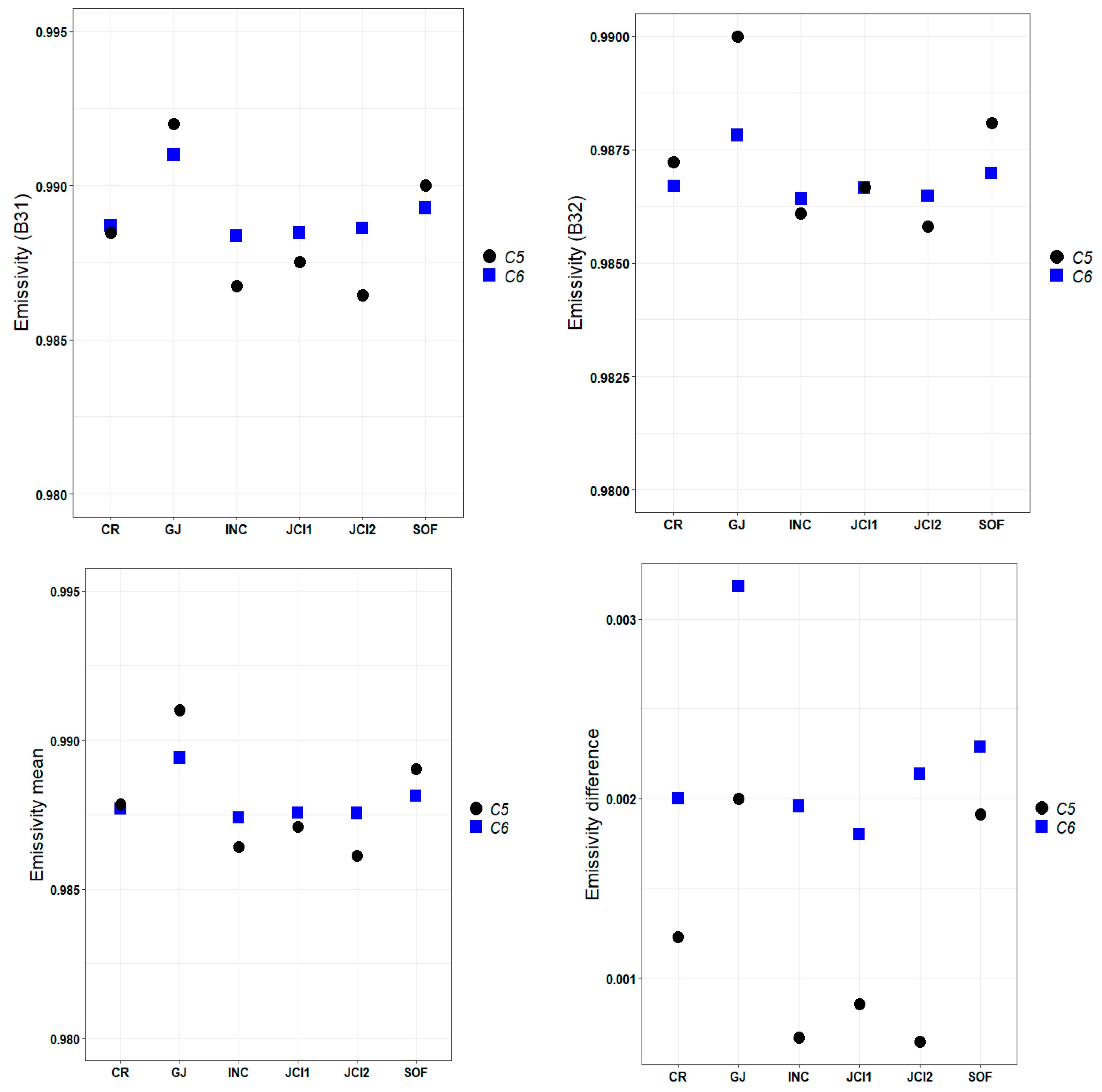
Previous studies have suggested that the better results obtained with C6 compared to C5 could be related to the improvements in MODIS emissivity data. Taking into account the importance of emissivity to estimate LST from satellites [86], we compared the C5 and C6 mean emissivity values of bands 31 and 32, as well as the mean and the difference of both bands for all stations (Figure 6, Figure 7, Figure 8 and Figure 9), except for GDC, for which we did not have C5 data. We included the mean and the difference because they were both parts of the equation for calculating MODIS LST using the GSW. The emissivity value of each band for each station was calculated, following the criteria of previous studies [56], as the average of the emissivity values for the entire study period using the dates with data after applying all of the filters described in Section 2.3.

As is well known, emissivity varies with wavelength or soil type, although it has also been suggested that soil moisture or surface viewing geometry may influence it [87]. Specifically, on snow-covered surfaces, the emissivity varies with depth, density and grain size [51,88]. The behavior described by Salisbury et al. [89] was that the snow emissivity decreased both with increasing particle size and with increasing snow density, while melting contributed to an increase in emissivity. However, it is very difficult to analyze the effects of grain size change on snow emissivity, since such information is not available on a large scale [90].

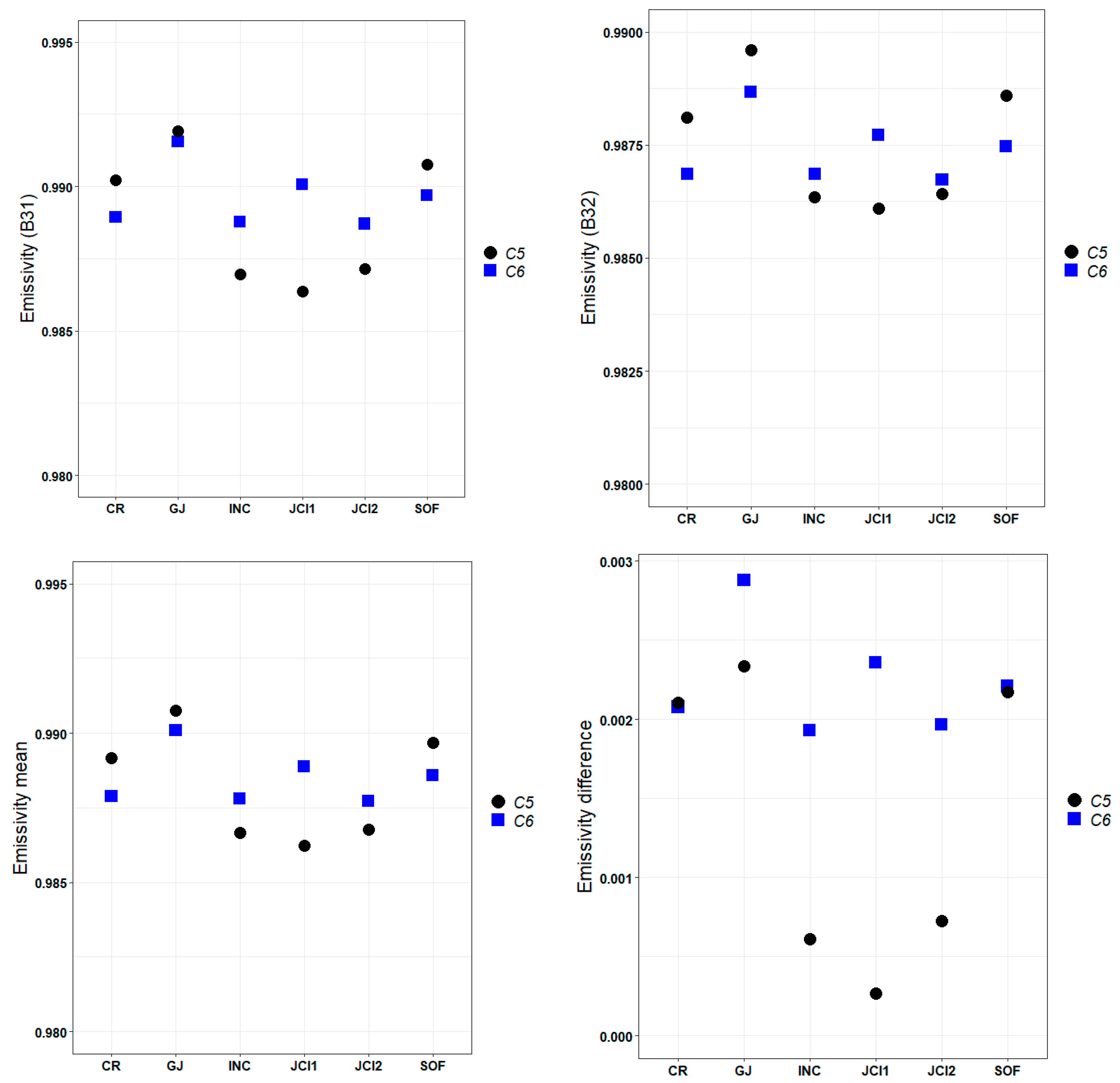
Figure 6 shows the mean emissivity values of bands 31 and 32, as well as the mean and the difference of both bands for each station for daytime Terra data with C5 and C6. The values of bands 31 and 32 are in the same range in both collections (band 31: between 0.989 and 0.992 and band 32: between 0.987 and 0.989). In the case of the means of both bands, the behaviors of C5 and C6 are also very similar: in INC2 and JCI2, both collections present the same value (0.988) and in the rest of the stations the C5 values are far from those of C6 only in |0.001|. Regarding the differences (band 31–band 32), the results of both collections are very close for all stations, especially for CR, SOF and JG, where C5 and C6 are separated by 0.0002, 0.0003 and −0.0004, respectively. If we examine R² values of Terra C6 daytime data for the different stations on Livingston Island, we find that the best agreement occurs in JCI2 (R² = 0.78), followed by CR (R² = 0.77), INC2 (R² = 0.73), SOF (R² = 0.71), JCI1 (R² = 0.68) and JG (R² = 0.64). On the other hand, with C5 values, the simple linear regression between MODIS LST and T_a of each station shows a low R² for all the stations (R² ≤ 0.4), values that, at least taking these data into account, would not be justified by problems only related to emissivity in C5.

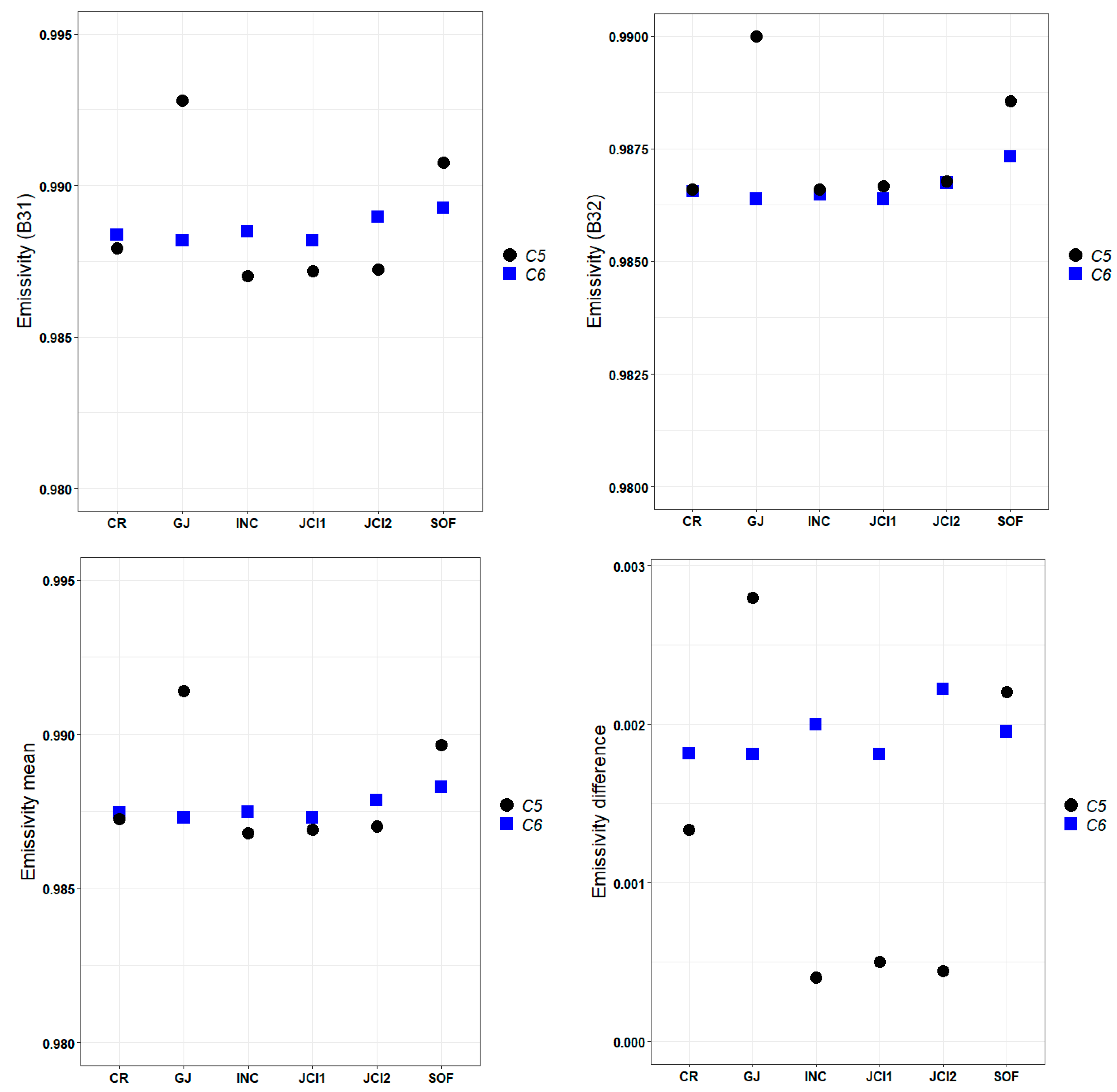
Figure 7 shows C5 and C6 emissivity values with Terra nighttime data. The values from both collections are still very close. For example, in the case of the band 32 values (to the right, top, in the figure) and the band 31 and 32 mean values (to the left, bottom, in the figure) the differences between the emissivity values of both collections for all stations are in the range of 0 to |0.001|, except for station GJ, where it is 0.002. Emissivity values with the Aqua data are shown in Figure 8. The difference between the values of bands 31 and 32 (to the right, bottom, in the figure) is in the range of 0 (CR and SOF) to −0.002 (JCI1). In addition, when analyzing the mean of both bands (to the left, below, in the figure) we find that at all the stations C5 and C6 values are separated by |0.001|, except for JCI1, where the C6 mean values exceed that of C5 by 0.003. Finally, Figure 9 shows the results for the Aqua nighttime data, where C5 and C6 emissivity behavior is also similar. For example, the mean values of both bands (to the left, bottom, in the figure) differ in this case in both collections in the range 0 to |0.001|, except in JG, where the value of C5 exceeds that of C6 by 0.004. In all cases, the JG value is not representative due to the lack of nighttime Aqua data at this station.

As can be seen, the discrepancies in the emissivity values are not conclusive to explain the better or worse correlation of MODIS LST with respect to the in situ data, either separately from the values of bands 31 and 32 nor from their means and differences. Although Wan [52] indicated that the GSW algorithm is more sensitive to the change in the difference in emissivity values in bands 31 and 32 than to the change in their mean, this behavior is not evident in our data, because although the correspondence with the in situ data is worse with the C5 data, there are no big differences in the emissivity behavior for both collections. It has been described that the highest and most unreliable uncertainties in emissivity are found beyond the 10.50 µm to 12.50 µm atmospheric window that MODIS uses for GSW algorithm retrievals [91]. This allows us to state that, for our data, the emissivity of the surface is not the main factor that generates the discrepancy between the MODIS LST of C5 and C6, which is consistent with what was described by Duan et al. [56].

The stations where MODIS achieves the best agreement with the in situ data are, in this order, GDC2 (R² = 0.82, with Terra daytime data), CR (R² = 0.81, with Terra and Aqua daytime data) and JCI2 (R² = 0.80, using Terra daytime data). In these stations, R² values contrast with those obtained for the study area with data from C5, where the R² average is 0.53 (with daytime data), being even lower with nighttime data (R² average = 0.49) [64]. Our results are also superior to those obtained in other studies estimating T_a from MODIS LST for Antarctica, such as Meyer et al. [28], who also used other variables besides to LST, with data from 32 stations distributed in continental Antarctica (R² = 0.78) and in two of the stations studied by Wang et al. [30] in the Lambert Glacier Basin in East Antarctica using MODIS daytime LST data (LGB00 and LGB20, with R² = 0.62 and R² = 0.74, respectively).

With respect to cross-validation, as in the case of C5 data [64], the worst results are also obtained with C6 with the nighttime data. The problems that MODIS presents in cloud detection have already been commented on in previous sections. The validation of the two unique models confirms that our results are within the range of values obtained with the MODIS LST product assessment for Antarctica and other study areas. Thus, for example, if we compare our results with the model obtained by Shi et al. [92] using LST MODIS data at nine sites around the world—America (3), Europe (1), Africa (1), Oceania (2) and Asia (2)—we can see that while our R²_CV average values (0.69 for the model that excludes the GDC2 station and 0.68 including it) are lower than the average value obtained in these nine regions (R² = 0.93), these authors reported higher errors (MAE = 2.1 °C, RMSE = 2.7 °C) than those obtained in our study in the cross-validation with daytime data (MAE_CV = 1.60 °C and 2.00 °C, RMSE_CV = 2.19 °C and 2.61 °C, in the unique model without GDC2; MAE_CV = 1.61 °C and 1.99 °C, RMSE_CV = 2.18 °C and 2.59 °C, in the unique model with GDC2). MODIS LST products have also been evaluated, for example, in Northeast China by Yang et al. [93], who obtained the following results with their best model for T_a average: R² = 0.94, RMSE = 3.60 °C and MAE = 2.80 °C. As can be seen, although R²_CV values obtained here are lower than those obtained in other study areas, cross-validation yields smaller errors, which is indicative of the performance of the models we evaluated.

Specifically in polar areas, in the Arctic, Westermann et al. [79] found deviations from weekly averages with MODIS LST data versus Svalbard in situ data to be less than 2 K, which is consistent with the MAE_CV average value obtained here for all data (1.99 ° C and 2.03 °C for the models without GDC2 and with GDC2, respectively), and especially excepting Aqua nighttime data (1.9 °C for both models). Similarly, our results yield a RMSE_CV average (2.59 °C and 2.63 °C, in the unique model, without GDC2, and including it, respectively), which is consistent with the 3 K error between MODIS LST and temperature of surface measured in situ during the period between 2002 and 2009, also in Svalbard by Westermann et al. [94]. Note that, on the one hand, higher errors would be expected in our study area, given the differences between T_a and surface temperature, and that, furthermore, we could expect even worse agreements given the range of temperatures in SSI, since the performance of MODIS measurements degrades as LST values increase and approach 0 °C [94].

Specifically in the studies on Antarctica, Meyer et al. [28] obtained as best results an R²_CV value of 0.71 and an RMSE_CV of 10.51 °C, with T_a data from 32 stations distributed in continental Antarctica. In the case of R²_CV, although its results are slightly higher than those obtained here for all data (R²_CV average = 0.69 and 0.68, in the unique model without GDC2 and with that station, respectively), our daytime data show better agreement in both cases (R²_CV = 0.75 and 0.73, Terra and Aqua, respectively). On the other hand, our errors, calculated from RMSE_CV are significantly lower, since they are in a range between 2 °C and 3 °C, except with Aqua nighttime data, which, however, do not exceed 3.13 °C. Regarding the MAE_CV, our errors do not exceed 2 °C, except with Terra nighttime data in the model without GDC2 and with Terra and Aqua nighttime data in the model with GDC2. These error values are also below the 3.4 °C obtained by Wang et al. 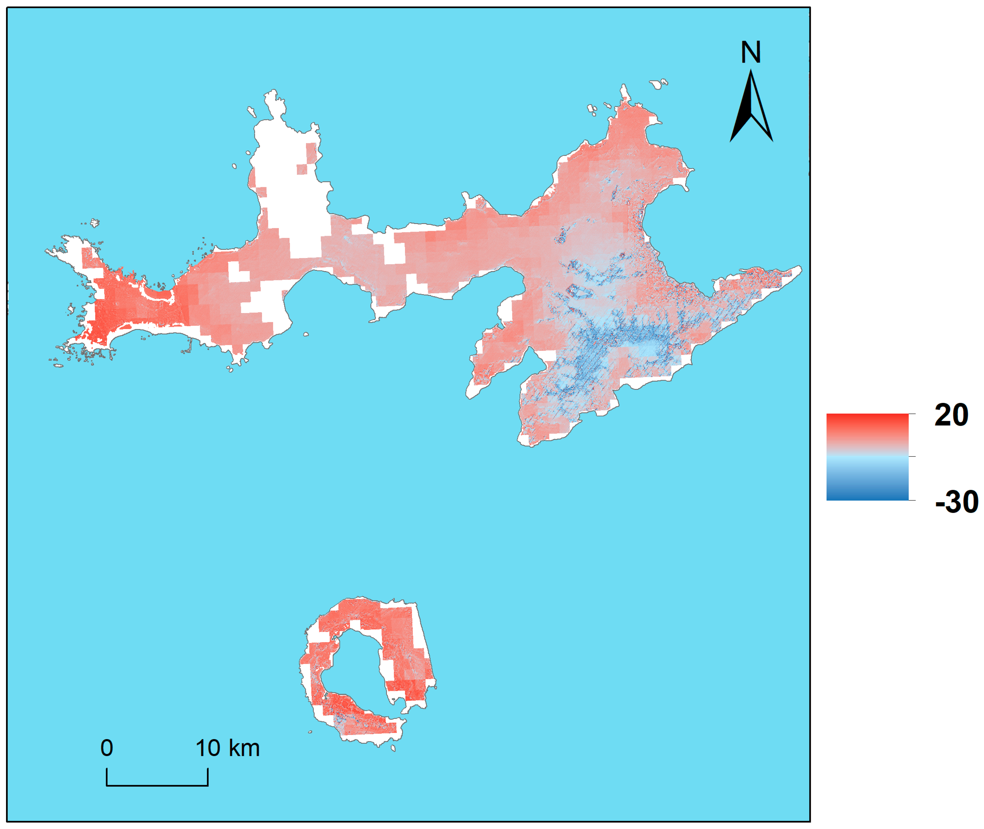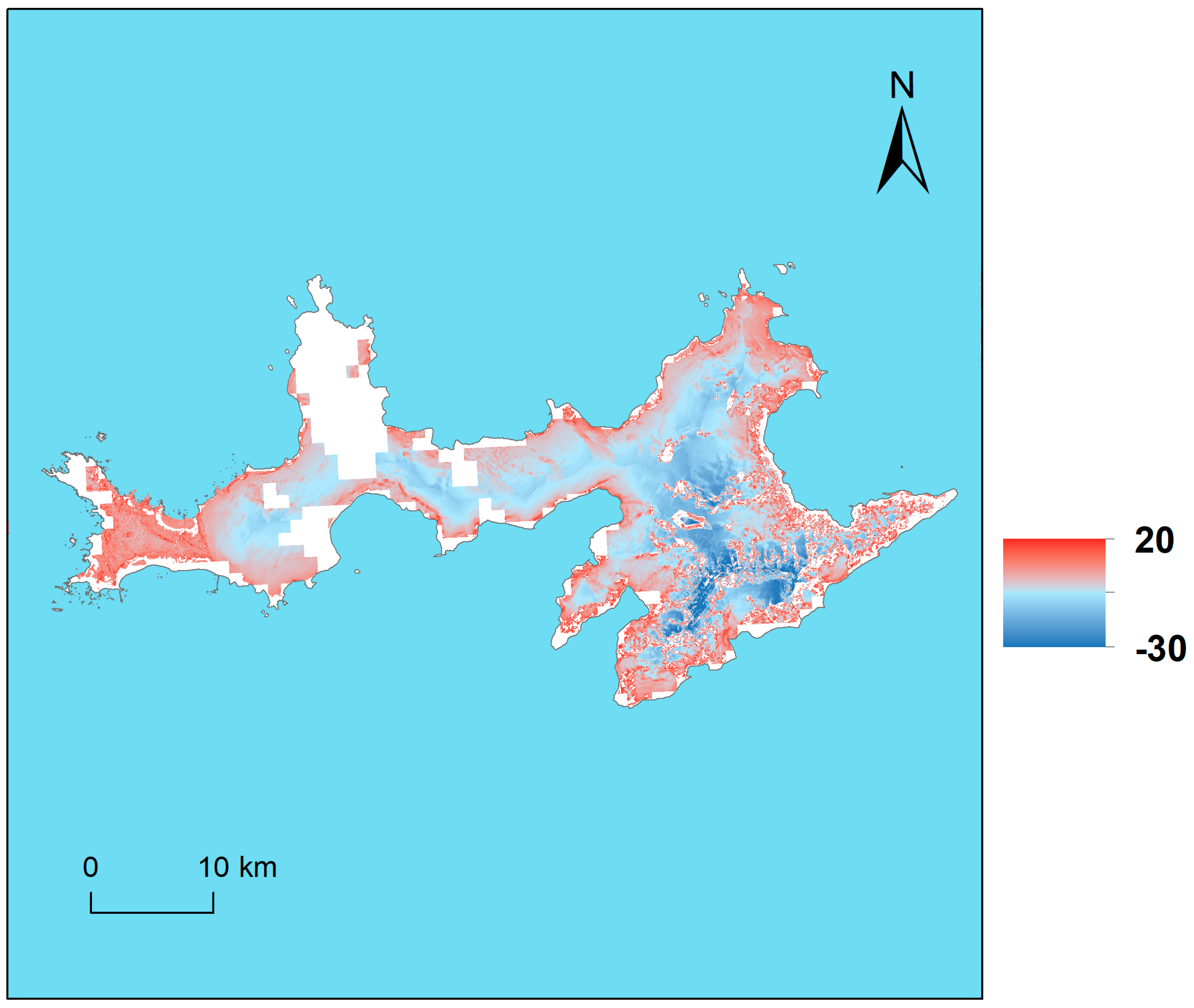[30] from the mean of the standard deviation of the differences between LST MODIS and T_a with data from the Lambert Glacier Basin. Another factor that should be taken into account when evaluating the performance of the models obtained here is that MODIS LST daily products provide data with a spatial resolution of 1 km. At both the Livingston and Deception Islands there is the advantage that at most sites there are no pixel coverage differences, thus minimizing the problem of surface coverage heterogeneity that has been noted as a potential biasing factor for MODIS LST studies in permafrost areas [79].

5. Conclusions

In this study, we estimated T_a from daytime and nighttime C6 MODIS LST data at sites in the SSI archipelago, in Maritime Antarctica, using empirical models. We obtained a clear improvement in the estimation Ta from LST using C6 over C5. The abundant cloudiness that affects latitudes below 60°S made it necessary to use high temporal resolution satellites/sensors, and MODIS data were thus appropriate. With Terra and Aqua LST MODIS data, R² averages of 0.73 and 0.56 were obtained with the daytime and nighttime data, respectively. In addition, errors were consistent with the results of the correlation between both variables, in different study areas and also with other satellites and/or sensors and constituted evidence of the good agreement between T_a and LST, taking into account the difference between both variables. The addition of predictive variables improved the correlations provided that at least one of them was significant. The best results were obtained with Terra daytime data. In addition, RSE values were, at all stations, except at JCI1 and GDC2, at the precision level considered exact (from 1 to 2 °C).

The unique models improved the correlation and reduced the errors with respect to the results obtained at some stations. However, although the application of a unique model did not allow the same level of accuracy to be achieved for the estimation of T_a in all cases, it did describe the behavior of temperature in Maritime Antarctica, where it is not possible to install and maintain a dense network of weather stations. In general, the results of the cross-validation corroborated the improvements obtained. In summary, regardless of the fact that future improvements in MODIS products should pay special attention to the distinction between snow and thin clouds, which would allow for improvements in cloud mask algorithms, the satisfactory results obtained here with the applied filters indicate that MODIS data can be used to study T_a in the area, as these filters contribute to the reduction of uncertainties in the modeling of T_a from satellites.

References

1. World Meteorological Organization. Guide to Instruments and Methods of Observation. Volume I: Measurement of Meteorological Variables; WMO: Geneva, Switzerland, 2018; Volume I, ISBN 9789263100085. [Google Scholar]
2. Wylie, R.G.; Lalas, T. Measurement of Temperature and Humidity. Specification, Construction, Properties and Use of the WMO Reference Psychrometer; Secretariat of the World Meteorological Organization: Geneva, Switzerland, 1992; ISBN 92-63-10759-9. [Google Scholar]
3. Anderson, M.C.; Norman, J.M.; Kustas, W.P.; Houborg, R.; Starks, P.J.; Agam, N. A thermal-based remote sensing technique for routine mapping of land-surface carbon, water and energy fluxes from field to regional scales. Remote Sens. Environ. 2008, 112, 4227–4241. [Google Scholar] [CrossRef]
4. Kalma, J.D.; McVicar, T.R.; McCabe, M.F. Estimating land surface evaporation: A review of methods using remotely sensed surface temperature data. Surv. Geophys. 2008, 29, 421–469. [Google Scholar] [CrossRef]
5. Li, Z.L.; Tang, B.H.; Wu, H.; Ren, H.; Yan, G.; Wan, Z.; Trigo, I.F.; Sobrino, J.A. Satellite-derived land surface temperature: Current status and perspectives. Remote Sens. Environ. 2013, 131, 14–37. [Google Scholar] [CrossRef]
6. Qie, Y.; Wang, N.; Wu, Y.; Chen, A. Variations in winter surface temperature of the Purog Kangri Ice Field, Qinghai-Tibetan Plateau, 2001–2018, using MODIS data. Remote Sens. 2020, 12, 1133. [Google Scholar] [CrossRef]
7. Wu, Y.; Wang, N.; He, J.; Jiang, X. Estimating mountain glacier surface temperatures from Landsat-ETM+ thermal infrared data: A case study of Qiyi glacier, China. Remote Sens. Environ. 2015, 163, 286–295. [Google Scholar] [CrossRef]
8. Zhang, R.; Tian, J.; Su, H.; Sun, X.; Chen, S.; Xia, J. Two improvements of an operational two-layer model for terrestrial surface heat flux retrieval. Sensors 2008, 8, 6165–6187. [Google Scholar] [CrossRef] [PubMed]
9. Hrbáček, F.; Láska, K.; Engel, Z. Effect of Snow Cover on the Active-Layer Thermal Regime. A Case Study from James Ross Island, Antarctic Peninsula. Permafr. Periglac. Process. 2016, 315, 307–315. [Google Scholar] [CrossRef]
10. Medley, B.; Thomas, E.R. Increased snowfall over the Antarctic Ice Sheet mitigated twentieth-century sea-level rise. Nat. Clim. Chang. 2019, 9, 34–39. [Google Scholar] [CrossRef]
11. Benali, A.; Carvalho, A.C.; Nunes, J.P.; Carvalhais, N.; Santos, A. Estimating air surface temperature in Portugal using MODIS LST data. Remote Sens. Environ. 2012, 124, 108–121. [Google Scholar] [CrossRef]
12. Hachem, S.; Duguay, C.R.; Allard, M. Comparison of MODIS-derived land surface temperatures with ground surface and air temperature measurements in continuous permafrost terrain. Cryosphere 2012, 6, 51–69. [Google Scholar] [CrossRef]
13. Washburn, A.L. Permafrost Features as Evidence of Climatic Change. Earth-Sci. Rev. 1980, 15, 327–402. [Google Scholar] [CrossRef]
14. Beltrami, H. Active Layer Distortion of Annual Air/Soil Thermal Orbits. Permafr. Periglac. Process. 1996, 7, 101–110. [Google Scholar] [CrossRef]
15. Mann, M.E.; Schmidt, G.A. Ground vs. surface air temperature trends: Implications for borehole surface temperature reconstructions. Geophys. Res. Lett. 2003, 30, 1607. [Google Scholar] [CrossRef]
16. Jin, M.; Dickinson, R.E.; Vogelmann, A.M. A Comparison of CCM2–BATS Skin Temperature and Surface-Air Temperature with Satellite and Surface Observations. J. Clim. 1997, 10, 1505–1524. [Google Scholar] [CrossRef]
17. Sun, J.; Mahrt, L. Determination of Surface Fluxes from the Surface Radiative Temperature. J. Atmos. Sci. 1995, 52, 1096–1106. [Google Scholar] [CrossRef]
18. Bahari, N.I.S.; Muharam, F.M.; Zulkafli, Z.; Mazlan, N. Modified Linear Scaling and Quantile Mapping Mean Bias Correction of MODIS Land Surface Temperature for Surface Air Temperature Estimation for the Lowland Areas of Peninsular Malaysia. Remote Sens. 2021, 13, 2589. [Google Scholar] [CrossRef]
19. Jin, M.; Dickinson, R.E. Land surface skin temperature climatology: Benefitting from the strengths of satellite observations. Environ. Res. Lett. 2010, 5, 044004. [Google Scholar] [CrossRef]
20. Shen, S.; Leptoukh, G.G. Estimation of surface air temperature over central and eastern Eurasia from MODIS land surface temperature. Environ. Res. Lett. 2011, 6, 045206. [Google Scholar] [CrossRef]
21. Scambos, T.A.; Campbell, G.G.; Pope, A.; Haran, T.; Muto, A.; Lazzara, M.; Reijmer, C.H.; van den Broeke, M.R. Ultralow Surface Temperatures in East Antarctica From Satellite Thermal Infrared Mapping: The Coldest Places on Earth. Geophys. Res. Lett. 2018, 45, 6124–6133. [Google Scholar] [CrossRef]
22. Sobrino, J.A.; Julien, Y.; García-Monteiro, S. Surface Temperature of the Planet Earth from Satellite Data. Remote Sens. 2020, 12, 218. [Google Scholar] [CrossRef]
23. Jin, M.; Dickinson, E. A generalized algorithm for retrieving cloudy sky skin temperature from satellite thermal infrared radiances. J. Geophys. Res. 2000, 105, 27037–27047. [Google Scholar] [CrossRef]
24. Prihodko, L.; Goward, S.N. Estimation of Air Temperature from Remotely Sensed Surface Observations. Remote Sens. Environ. 1997, 60, 335–346. [Google Scholar] [CrossRef]
25. Urban, M.; Eberle, J.; Hüttich, C.; Schmullius, C.; Herold, M. Comparison of Satellite-Derived Land Surface Temperature and Air Temperature from Meteorological Stations on the Pan-Arctic Scale. Remote Sens. 2013, 5, 2348–2367. [Google Scholar] [CrossRef]
26. Mostovoy, G.V.; King, R.L.; Reddy, K.R.; Kakani, V.G.; Filipova, M. Statistical Estimation of Daily Maximum and Minimum Air Temperatures from MODIS LST Data over the State of Mississippi Statistical Estimation of Daily Maximum and over the State of Mississippi. GISci. Remote Sens. 2013, 43, 78–110. [Google Scholar] [CrossRef]
27. Vancutsem, C.; Ceccato, P.; Dinku, T.; Connor, S.J. Evaluation of MODIS land surface temperature data to estimate air temperature in different ecosystems over Africa. Remote Sens. Environ. 2010, 114, 449–465. [Google Scholar] [CrossRef]
28. Meyer, H.; Katurji, M.; Appelhans, T.; Müller, M.U.; Nauss, T.; Roudier, P.; Zawar-Reza, P. Mapping Daily Air Temperature for Antarctica Based on MODIS LST. Remote Sens. 2016, 8, 732. [Google Scholar] [CrossRef]
29. Obu, J.; Westermann, S.; Vieira, G.; Abramov, A.; Ruby Balks, M.; Bartsch, A.; Hrbáček, F.; Kääb, A.; Ramos, M. Pan-Antarctic map of near-surface permafrost temperatures at 1km2 scale. Cryosphere 2020, 14, 497–519. [Google Scholar] [CrossRef]
30. Wang, Y.; Wang, M.; Zhao, J. A Comparison of MODIS LST Retrievals with in Situ Observations from AWS over the Lambert Glacier Basin, East Antarctica. Int. J. Geosci. 2013, 4, 611–617. [Google Scholar] [CrossRef]
31. Marshall, G.J.; Orr, A.; van Lipzig, N.P.M.; King, J.C. The Impact of a Changing Southern Hemisphere Annular Mode on Antarctic Peninsula Summer Temperatures. J. Clim. 2006, 19, 5388–5404. [Google Scholar] [CrossRef]
32. Massom, R.A.; Stammerjohn, S.E.; Smith, R.C.; Pook, M.J.; Iannuzzi, R.A.; Adams, N.; Martinson, D.G.; Vernet, M.; Fraser, W.R.; Quetin, L.B.; et al. Extreme Anomalous Atmospheric Circulation in the West Antarctic Peninsula Region in Austral Spring and Summer 2001/02, and Its Profound Impact on Sea Ice and Biota. J. Clim. 2006, 19, 3544–3571. [Google Scholar] [CrossRef]
33. Oliva, M.; Navarro, F.; Hrbáček, F.; Hernández, A.; Nývlt, D.; Pereira, P.; Ruiz-Fernández, J.; Trigo, R. Recent regional climate cooling on the Antarctic Peninsula and associated impacts on the cryosphere. Sci. Total Environ. 2017, 580, 210–223. [Google Scholar] [CrossRef]
34. Turner, J.; Colwell, S.R.; Marshall, G.J.; Lachlan-Cope, T.A.; Carleton, A.M.; Jones, P.D.; Lagun, V.; Reid, P.A.; Iagovkina, S. Antarctic climate change during the last 50 years. Int. J. Climatol. 2005, 25, 279–294. [Google Scholar] [CrossRef]
35. Gonzalez, S.; Vasallo, F.; Recio-Blitz, C.; Guijarro, J.A.; Riesco, J. Atmospheric patterns over the Antarctic Peninsula. J. Clim. 2018, 31, 3597–3608. [Google Scholar] [CrossRef]
36. Turner, J.; Marshall, G.J.; Phillips, T.; Lu, H.; Clem, K.; Colwell, S. Antarctic temperature variability and change from station data. Int. J. Climatol. 2020, 40, 2986–3007. [Google Scholar] [CrossRef]
37. Stastna, V. Spatio-temporal changes in surface air temperature in the region of the northern Antarctic Peninsula and South Shetland Islands during 1950–2003. Polar Sci. 2010, 4, 18–33. [Google Scholar] [CrossRef]
38. Kejna, M. Trends of air temperature of the Antarctic during the period 1958–2000. Polish Polar Res. 2003, 24, 99–126. [Google Scholar]
39. King, J.C.; Comiso, J.C. The spatial coherence of interannual temperature variations in the Antarctic Peninsula. Geophys. Res. Lett. 2003, 30, 1040. [Google Scholar] [CrossRef]
40. King, J.C.; Turner, J.; Marshall, G.J.; Connolley, W.M.; Lachlan-Cope, T.A. Antarctic Peninsula climate variability and its causes as revealed by analysis of instrumental records. Antarct. Res. Ser. 2003, 79, 17–30. [Google Scholar] [CrossRef]
41. Morris, E.M.; Vaughan, D.G. Spatial and Temporal Variation of Surface Temperature on the Antarctic Peninsula And The Limit of Viability of Ice Shelves. Antarct. Res. Ser. 2003, 79, 61–68. [Google Scholar] [CrossRef]
42. Thompson, D.W.J.; Solomon, S. Interpretation of Recent Southern Hemisphere Climate Change. Science 2002, 296, 895–899. [Google Scholar] [CrossRef]
43. Orr, A.; Cresswell, D.; Marshall, G.J.; Hunt, J.C.R.; Sommeria, J.; Wang, C.G.; Light, M. A ‘low-level’ explanation for the recent large warming trend over the western Antarctic Peninsula involving blocked winds and changes in zonal circulation. Geophys. Res. Lett. 2004, 31, L06204. [Google Scholar] [CrossRef]
44. Steig, E.J.; Schneider, D.P.; Rutherford, S.D.; Mann, M.E.; Comiso, J.C.; Shindell, D.T. Warming of the Antarctic ice-sheet surface since the 1957 International Geophysical Year. Nature 2009, 457, 459–462. [Google Scholar] [CrossRef]
45. Bañón, M.; Vasallo, F. Aemet en la Antártida: Climatología y Meteorología Sinóptica en las Estaciones Meteorológicas en las Estaciones Meteorológicas Españolas en la Antártida; AEMET: Madrid, Spain, 2015. [Google Scholar]
46. Rubin, M.J. Preface. In Studies in Antarctic Meteorology; American Geophysical Union: Washington, DC, USA, 1966; p. V. [Google Scholar]
47. Vieira, G.; Bockheim, J.; Guglielmin, M.; Balks, M.; Abramov, A.A.; Boelhouwers, J.; Cannone, N.; Ganzert, L.; Gilichinsky, D.A.; Goryachkin, S.; et al. Thermal State of Permafrost and Active-layer Monitoring in the Antarctic: Advances during the International Polar Year 2007–2009. Permafr. Periglac. Process. 2010, 21, 182–197. [Google Scholar] [CrossRef]
48. Sobrino, J.A.; Raissouni, N.; Kerr, Y.; Olioso, A.; López-García, M.J.; El Kharraz, M.H.; Cuenca, J.; Dempere, L. Teledetección; Sobrino, J.A., Ed.; Servicio de Publicaciones, Universidad de Valencia: Valencia, Spain, 2000; ISBN 84-370-4220-8. [Google Scholar]
49. Wan, Z.; Zhang, Y.; Zhang, Q.; Lia, Z. Validation of the land-surface temperature products retrieved from Terra Moderate Resolution Imaging Spectroradiometer data. Remote Sens. Env. 2002, 83, 163–180. [Google Scholar] [CrossRef]
50. National Aeronautics and Space Administration (NASA) Moderate Resolution Imaging Spectroradiometer (MODIS). Available online: https://modis.gsfc.nasa.gov/about/specifications.php (accessed on 24 September 2023).
51. Wan, Z.; Dozier, J. A generalized split-window algorithm for retrieving land-surface temperature from space. IEEE Trans. Geosci. Remote Sens. 1996, 34, 892–905. [Google Scholar] [CrossRef]
52. Wan, Z. New refinements and validation of the collection-6 MODIS land-surface temperature/emissivity product. Remote Sens. Environ. 2014, 140, 36–45. [Google Scholar] [CrossRef]
53. Wan, Z. Collection-6 MODIS Land Surface Temperature Products Users’ Guide. Available online: https://lpdaac.usgs.gov/documents/118/MOD11_User_Guide_V6.pdf (accessed on 24 September 2023).
54. Gorelick, N.; Hancher, M.; Dixon, M.; Ilyushchenko, S.; Thau, D.; Moore, R. Google Earth Engine: Planetary-scale geospatial analysis for everyone. Remote Sens. Environ. 2017, 202, 18–27. [Google Scholar] [CrossRef]
55. Göttsche, F.-M.; Olesen, F.-S.; Bork-Unkelbach, A. Validation of land surface temperature derived from MSG/ SEVIRI with in situ measurements at Gobabeb, Namibia. Int. J. Remote Sens. 2013, 34, 3069–3083. [Google Scholar] [CrossRef]
56. Duan, S.-B.; Li, Z.-L.; Li, H.; Göttsche, F.-M.; Wu, H.; Zhao, W.; Leng, P.; Zhang, X.; Coll, C. Validation of Collection 6 MODIS land surface temperature product using in situ measurements. Remote Sens. Environ. 2019, 225, 16–29. [Google Scholar] [CrossRef]
57. Williamson, S.N.; Hik, D.S.; Gamon, J.A.; Jarosch, A.H.; Anslow, F.S.; Clarke, G.K.C.; Scott Rupp, T. Spring and summer monthly MODIS LST is inherently biased compared to air temperature in snow covered sub-Arctic mountains. Remote Sens. Environ. 2017, 189, 14–24. [Google Scholar] [CrossRef]
58. Ke, L.; Ding, X.; Song, C. Reconstruction of Time-Series MODIS LST in Central Qinghai-Tibet Plateau Using Geostatistical Approach. IEEE Geosci. Remote Sens. Lett. 2013, 10, 1602–1606. [Google Scholar] [CrossRef]
59. Ke, L.; Song, C.; Ding, X. Reconstructing Complete MODIS LST Based on Temperature Gradients in Northeastern Qinghai-Tibet Plateau. In Proceedings of the 2012 IEEE International Geoscience and Remote Sensing Symposium, Munich, Germany, 22–27 July 2012; pp. 3505–3508. [Google Scholar]
60. Ke, L.; Song, C. ISPRS Journal of Photogrammetry and Remote Sensing Remotely sensed surface temperature variation of an inland saline lake over the central Qinghai—Tibet Plateau. ISPRS J. Photogramm. Remote Sens. 2014, 98, 157–167. [Google Scholar] [CrossRef]
61. De Pablo, M.A.; Ramos, M.; Molina, A.; Vieira, G.; Hidalgo, M.A.; Prieto, M.; Jiménez, J.J.; Fernández, S.; Recondo, C.; Calleja, J.F.; et al. Frozen ground and snow cover monitoring in the South Shetland Islands, Antarctica: Instrumentation, effects on ground thermal behaviour and future research. Cuad. Investig. Geográfica 2016, 42, 475–495. [Google Scholar] [CrossRef]
62. De Pablo, M.A.; Jiménez, J.J.; Ramos, M.; Prieto, M.; Molina, A.; Vieira, G.; Hidalgo, M.A.; Fernández, S.; Recondo, C.; Calleja, J.F.; et al. Frozen Ground and Snow Cover Monitoring in Livingston and Deception Islands, Antarctica: Preliminary Results of the—PERMASNOW Project. Cuad. Investig. Geográfica 2020, 46, 187–222. [Google Scholar] [CrossRef]
63. Bañón, M.; AEMET, Madrid, Spain. Personal communication, 2017.
64. Recondo, C.; Corbea-Pérez, A.; Peón, J.; Pendás, E.; Ramos, M.; Calleja, J.F.; de Pablo, M.Á.; Fernández, S.; Corrales, J.A. Empirical Models for Estimating Air Temperature Using MODIS Land Surface Temperature (and Spatiotemporal Variables) in the Hurd Peninsula of Livingston Island, Antarctica, between 2000 and 2016. Remote Sens. 2022, 14, 3206. [Google Scholar] [CrossRef]
65. Earth Obervation Research Center JAXA ALOS Global Digital Surface Model “ALOS World 3D—30m (AW3D30)”. Available online: https://www.eorc.jaxa.jp/ALOS/en/dataset/aw3d30/aw3d30_e.htm (accessed on 21 June 2021).
66. Recondo, C.; Peón, J.J.; Zapico, E.; Pendás, E. Empirical models for estimating daily surface water vapour pressure, air temperature, and humidity using MODIS and spatiotemporal variables. Applications to peninsular Spain. Int. J. Remote Sens. 2013, 34, 8051–8080. [Google Scholar] [CrossRef]
67. Peón, J.; Recondo, C.; Calleja, J.F. Improvements in the estimation of daily minimum air temperature in peninsular Spain using MODIS land surface temperature. Int. J. Remote Sens. 2014, 35, 5148–5166. [Google Scholar] [CrossRef]
68. Felicísimo, A.M. Modelos Digitales del Terreno. Introducción y Aplicaciones en las Ciencias Ambientales; Pentalfa Ediciones: Oviedo, Spain, 1994. [Google Scholar]
69. Vieira, G.; López-Martínez, J.; Serrano, E.; Ramos, M.; Gruber, S.; Hauck, C.; Blanco, J.J. Geomorphological observations of permafrost and ground-ice degradation on Deception and Livingston Islands, Maritime Antarctica. In Proceedings of the 9th International Conference on Permafrost, Fairbanks, Alaska, 29 June–3 July 2008; Kane, D.L., Hinkel, K.M., Eds.; Institute of Northern Engineering: Fairbanks, AK, USA, 2008; pp. 1839–1844. [Google Scholar]
70. Melo, R.; Vieira, G.; Caselli, A.; Ramos, M. Geomorphology Susceptibility modelling of hummocky terrain distribution using the information value method (Deception Island, Antarctic Peninsula). Geomorphology 2012, 155–156, 88–95. [Google Scholar] [CrossRef]
71. Vera, L. Colonization and demographic structure of Deschampsia antarctica and Colobanthus quitensis along an altitudinal gradient on Living-ston Island, South Shetland Islands, Antarctica. Polar Res. 2011, 1, 113735. [Google Scholar] [CrossRef]
72. Kawashima, S.; Ishida, T.; Minomura, M.; Miwa, T. Relations between Surface Temperature and Air Temperature on a Local Scale during Winter Nights. J. Appl. Meteorol. 2000, 39, 1570–1579. [Google Scholar] [CrossRef]
73. Ackerman, S.A.; Holz, R.E.; Frey, R.; Eloranta, E.W.; Maddux, B.C.; McGill, M. Cloud Detection with MODIS. Part II: Validation. J. Atmos. Ocean. Technol. 2008, 25, 1073–1086. [Google Scholar] [CrossRef]
74. Liu, Y.; Ackerman, S.A.; Maddux, B.C.; Key, J.R.; Frey, R.A. Errors in Cloud Detection over the Arctic Using a Satellite Imager and Implications for Observing Feedback Mechanisms. J. Clim. 2010, 23, 1894–1907. [Google Scholar] [CrossRef]
75. Østby, T.I.; Schuler, T.V.; Westermann, S. Severe cloud contamination of MODIS Land Surface Temperatures over an Arctic ice cap, Svalbard. Remote Sens. Environ. 2014, 142, 95–102. [Google Scholar] [CrossRef]
76. Wang, X.; Key, J.R. Recent Trends in Arctic Surface, Cloud, and Radiation Properties from Space. Science 2003, 299, 1725–1729. [Google Scholar] [CrossRef] [PubMed]
77. Wang, X.; Key, J.R. Arctic Surface, Cloud, and Radiation Properties Based on the AVHRR Polar Pathfinder Dataset. Part I: Spatial and Temporal Characteristics. J. Clim. 2005, 18, 2558–2574. [Google Scholar] [CrossRef]
78. Zhang, H.; Zhang, F.; Zhang, G.; He, X.; Tian, L. Evaluation of cloud effects on air temperature estimation using MODIS LST based on ground measurements over the Tibetan Plateau. Atmos. Chem. Phys. 2016, 16, 13681–13696. [Google Scholar] [CrossRef]
79. Westermann, S.; Langer, M.; Boike, J. Spatial and temporal variations of summer surface temperatures of high-arctic tundra on Svalbard—Implications for MODIS LST based permafrost monitoring. Remote Sens. Environ. 2011, 115, 908–922. [Google Scholar] [CrossRef]
80. Langer, M.; Westermann, S.; Boike, J. Remote Sensing of Environment Spatial and temporal variations of summer surface temperatures of wet polygonal tundra in Siberia—implications for MODIS LST based permafrost monitoring. Remote Sens. Environ. 2010, 114, 2059–2069. [Google Scholar] [CrossRef]
81. Corbea-Pérez, A.; Calleja, J.F.; Recondo, C.; Fernández, S. Evaluation of the MODIS (C6) Daily Albedo Products for Livingston Island, Antarctic. Remote Sens. 2021, 13, 2357. [Google Scholar] [CrossRef]
82. King, J.C.; Turner, J. Antarctic Meteorology and Climatology; Cambridge University Press: New York, NY, USA, 1997; ISBN 978-0-521-46560-1. [Google Scholar]
83. Angiel, P.J.; Potocki, M.; Biszczuk-Jakubowska, J. Weather condition characteristics at the H. Arctowski station (South Shetlands, Antarctica) for 2006, in comparison with multi-year research results. Misc. Geogr. 2010, 14, 79–89. [Google Scholar] [CrossRef]
84. Liu, H.; He, B.J.; Gao, S.; Zhan, Q.; Yang, C. Influence of non-urban reference delineation on trend estimate of surface urban heat island intensity: A comparison of seven methods. Remote Sens. Environ. 2023, 296, 113735. [Google Scholar] [CrossRef]
85. Liu, H.; Huang, B.; Cheng, X.; Yin, M.; Shang, C.; Luo, Y.; He, B.J. Sensing-based park cooling performance observation and assessment: A review. Build. Environ. 2023, 245, 110915. [Google Scholar] [CrossRef]
86. Becker, F. The impact of spectral emissivity on the measurement of land surface temperature from a satellite. Int. J. Remote Sens. 2007, 8, 1509–1522. [Google Scholar] [CrossRef]
87. Salisbury, J.W.; D’Aria, D.M. Emissivity of Terrestrial Materials in the 8–14 um Atmospheric Window. Remote Sens. Environ. 1992, 42, 83–106. [Google Scholar] [CrossRef]
88. McFarland, M.J.; Miller, R.L.; Neale, C.M.U. Land Surface Temperature Derived From the SSM/I Passive Microwave Brightness Temperatures. IEEE Trans. Geosci. Remote Sens. 1990, 28, 839–845. [Google Scholar] [CrossRef]
89. Salisbury, J.W.; D’Aria, D.M.; Wald, A. Measurements of thermal infrared spectral reflectance of frost, snow, and ice. J. Geophys. Res. 1994, 99, 24235–24240. [Google Scholar] [CrossRef]
90. Stroeve, J.; Steffen, K. Variability of AVHRR-Derived Clear-Sky Surface Temperature over the Greenland Ice Sheet. J. Appl. Meteorol. 1998, 37, 23–31. [Google Scholar] [CrossRef]
91. Pérez-Díaz, C.L.; Lakhankar, T.; Romanov, P.; Muñoz, J.; Khanbilvardi, R.; Yu, Y. Evaluation of MODIS land surface temperature with in-situ snow surface temperature from CREST- SAFE. Int. J. Remote Sens. 2017, 38, 4722–4740. [Google Scholar] [CrossRef]
92. Shi, S.; Helman, D.; Lensky, I.M. Worldwide continuous gap-filled MODIS land surface temperature dataset. Sci. Data 2021, 8, 74. [Google Scholar] [CrossRef]
93. Yang, Y.Z.; Cai, W.H.; Yang, J. Evaluation of MODIS Land Surface Temperature Data to Estimate Near-Surface Air Temperature in. Remote Sens. 2017, 9, 410. [Google Scholar] [CrossRef]
94. Westermann, S.; Langer, M.; Boike, J. Systematic bias of average winter-time land surface temperatures inferred from MODIS at a site on Svalbard, Norway. Remote Sens. Environ. 2012, 118, 162–167. [Google Scholar] [CrossRef]
Figure 1. Framework diagram of the study.
Remotesensing 16 01084 g001
Figure 2. Study area. Upper image, Antarctica; lower image, South Shetland Island (SSI) archipelago.
Remotesensing 16 01084 g002
Figure 3. RGB composites (4-3-2) of Landsat 8 (9 February 2020). Images are projected in WGS84 UTM20S. Above, image of Livingston Island; bottom left, zoom image of the Hurd Peninsula with stations Juan Carlos I (JCI), Reina Sofía (SOF), Johnsons Glacier (JG), Incinerador (INC) and Collado Ramos (CR), and, on the right, Deception Island with station Gabriel de Castilla (GDC). In the case of the stations that had two locations during the study period (JCI, INC and GDC), the current location is shown.
Remotesensing 16 01084 g003
Figure 4. Ta (°C) obtained with the unique model for Terra-Day (including GDC2 station) generated from C6 MOD11A1 data including spatiotemporal variables from the Terra-MODIS image of 16 January 2014. The figure shows Livingston and Deception Islands.
Remotesensing 16 01084 g004
Figure 5. Ta (°C) obtained with the unique model for Terra-Day (without GDC2 station) generated from C6 MOD11A1 data including spatiotemporal variables, from the Terra-MODIS image of 16 January 2014. The figure shows Livingston Island.
Remotesensing 16 01084 g005
Figure 6. Mean emissivity values of bands 31 (top, left) and 32 (top, right), as well as the mean (bottom, left) and difference (bottom, right) of both bands for each station for C5 and C6 Terra-day.
Remotesensing 16 01084 g006
Figure 7. Mean emissivity values of bands 31 (top, left) and 32 (top, right), as well as the mean (bottom, left) and difference (bottom, right) of both bands for each station for C5 and C6 Terra-night.
Remotesensing 16 01084 g007
Figure 8. Mean emissivity values of bands 31 (top, left) and 32 (top, right), as well as the mean (bottom, left) and difference (bottom, right) of both bands for each station for C5 and C6 Aqua-day.
Remotesensing 16 01084 g008
Figure 9. Mean emissivity values of bands 31 (top, left) and 32 (top, right), as well as the mean (bottom, left) and difference (bottom, right) of both bands for each station for C5 and C6 Aqua-night.
Remotesensing 16 01084 g009