
Environmental Influences on the Detection of Buried Objects with a Ground-Penetrating Radar


Abstract
1. Introduction
2. Theory
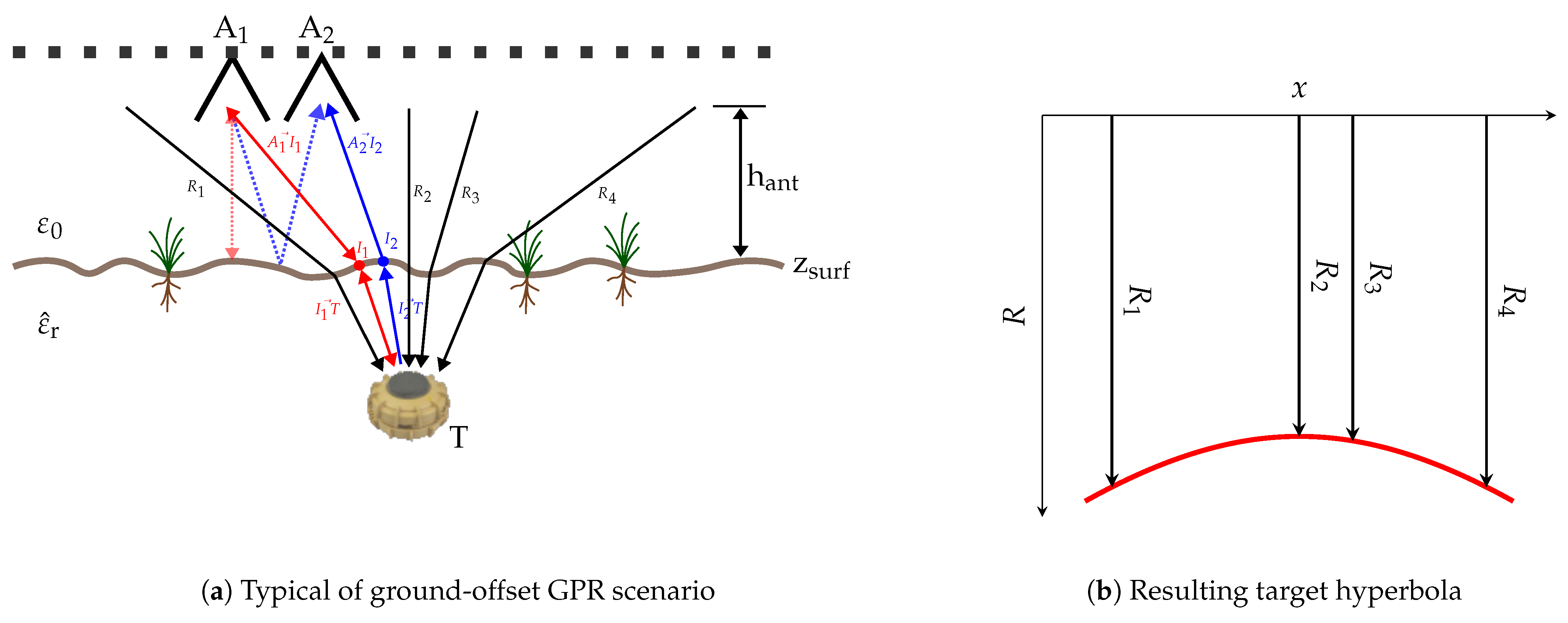
2.1. Radar Principles
2.1.1. SFCW-Radar
2.1.2. SFCW Target Phase
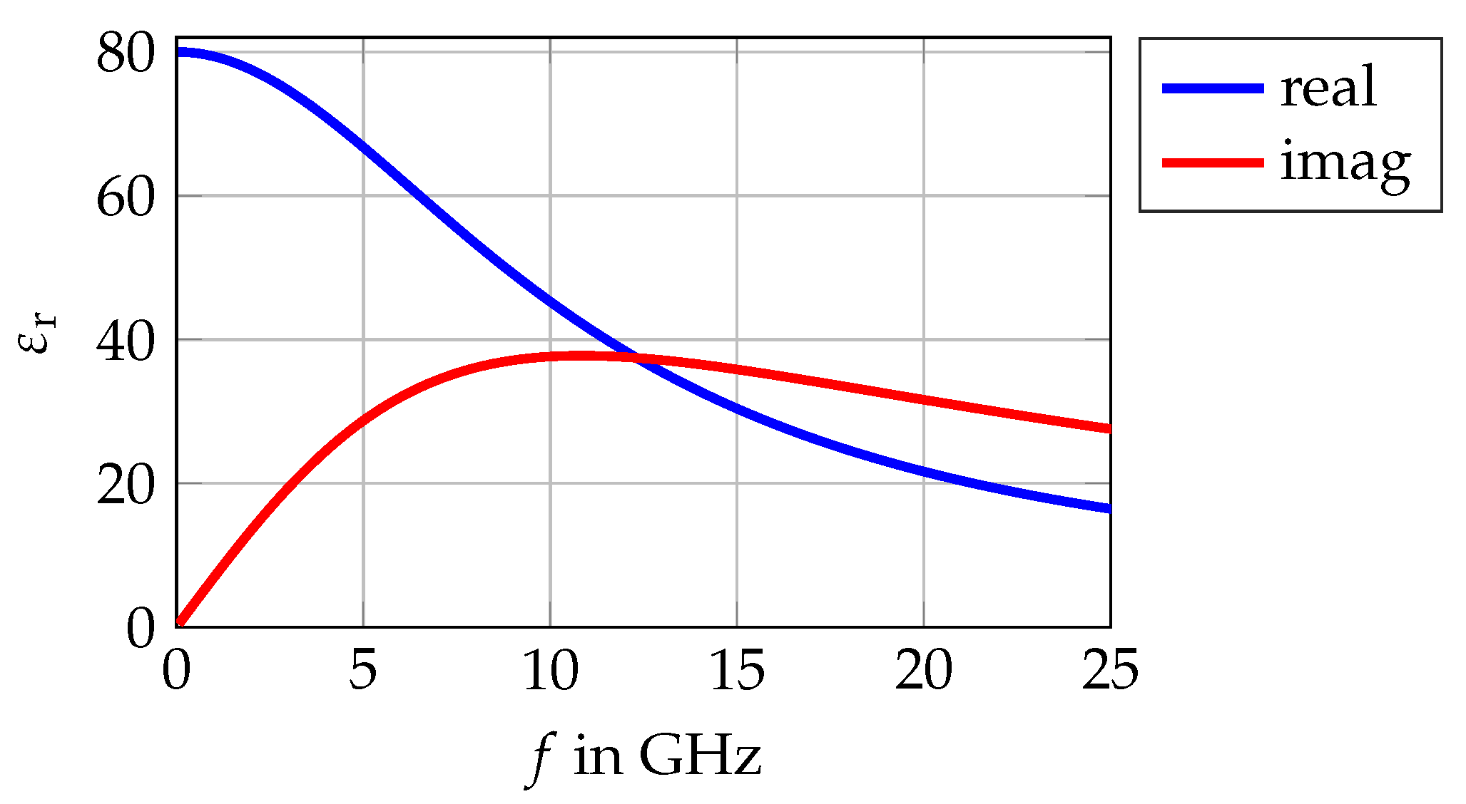
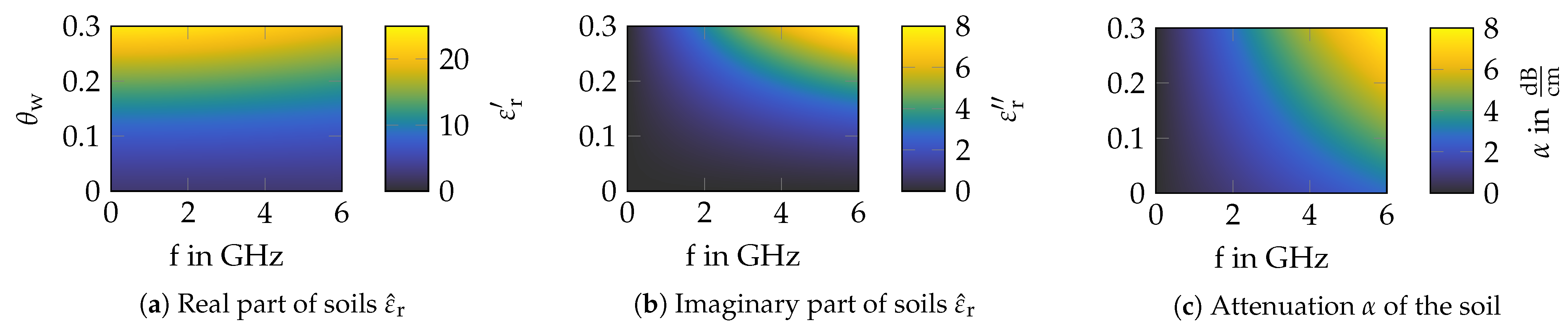
2.2. Soil Properties
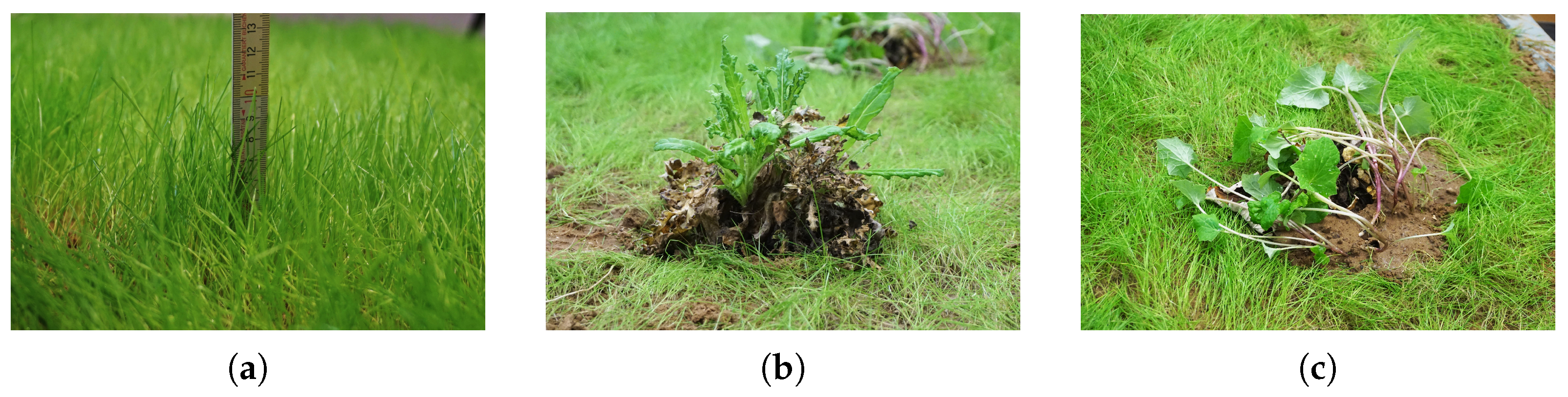
2.3. Vegetation
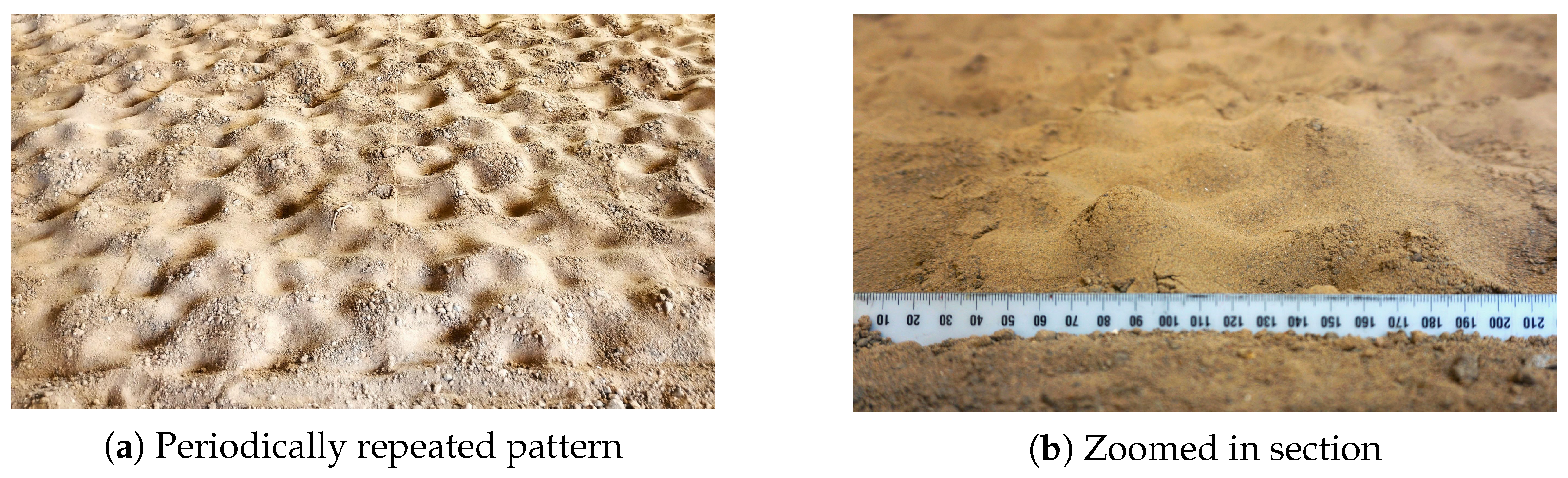
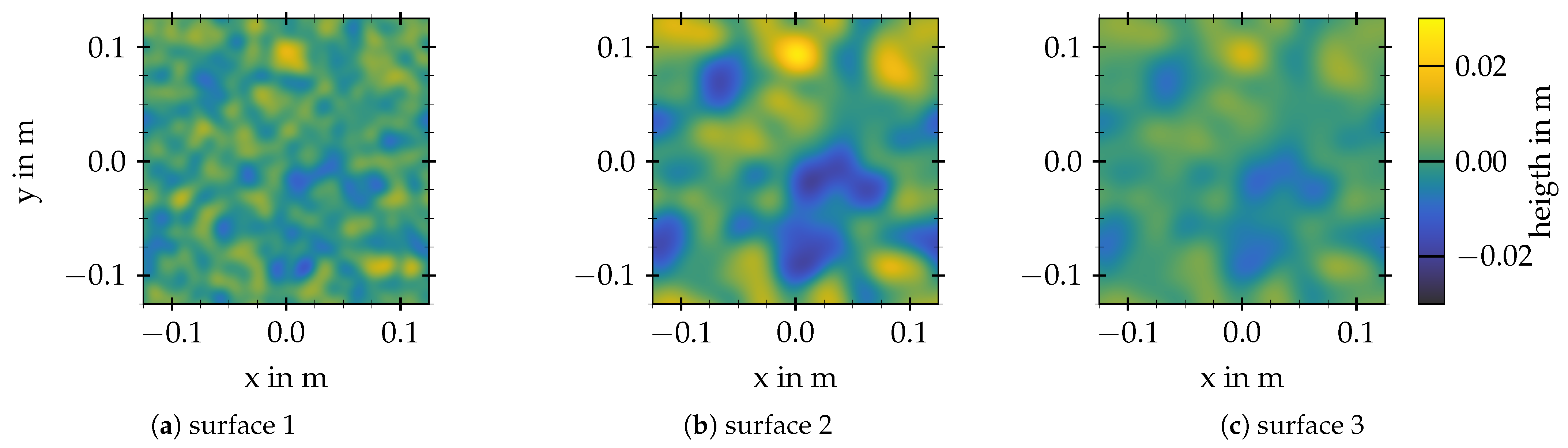
2.4. Surface Roughness
- (1)
- Rayleigh Criterion:
- (2)
- Fraunhofer Criterion:
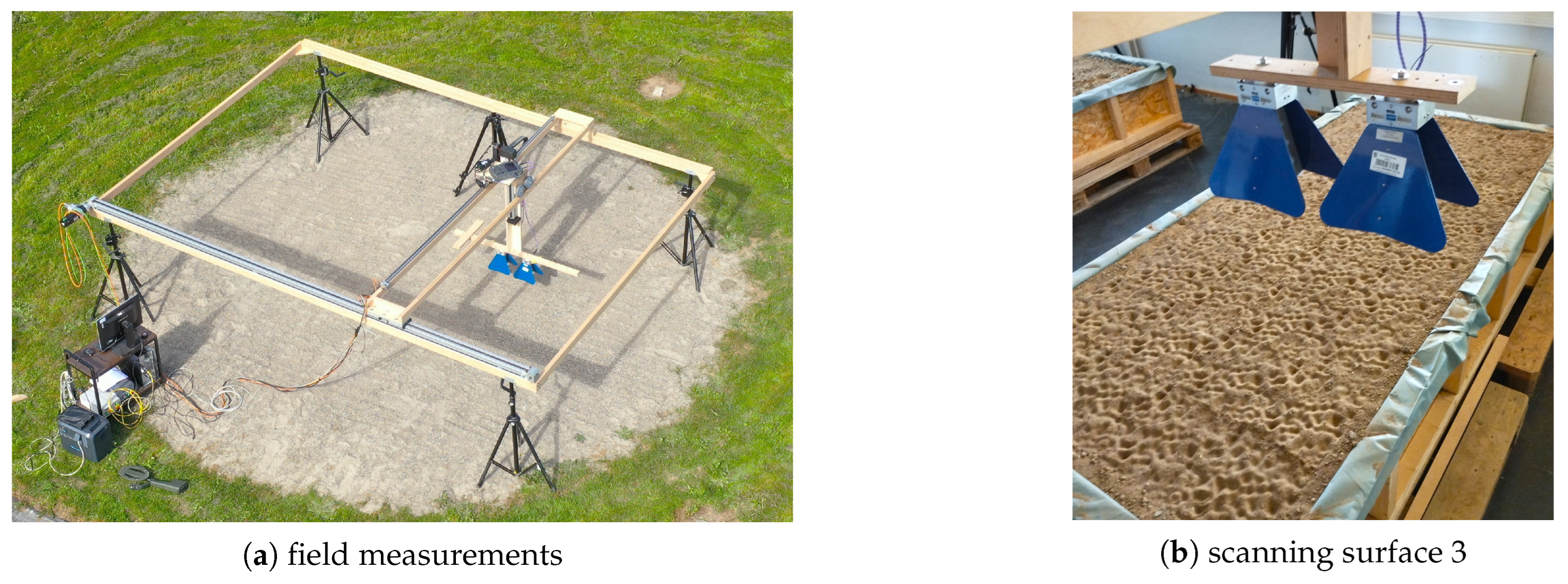
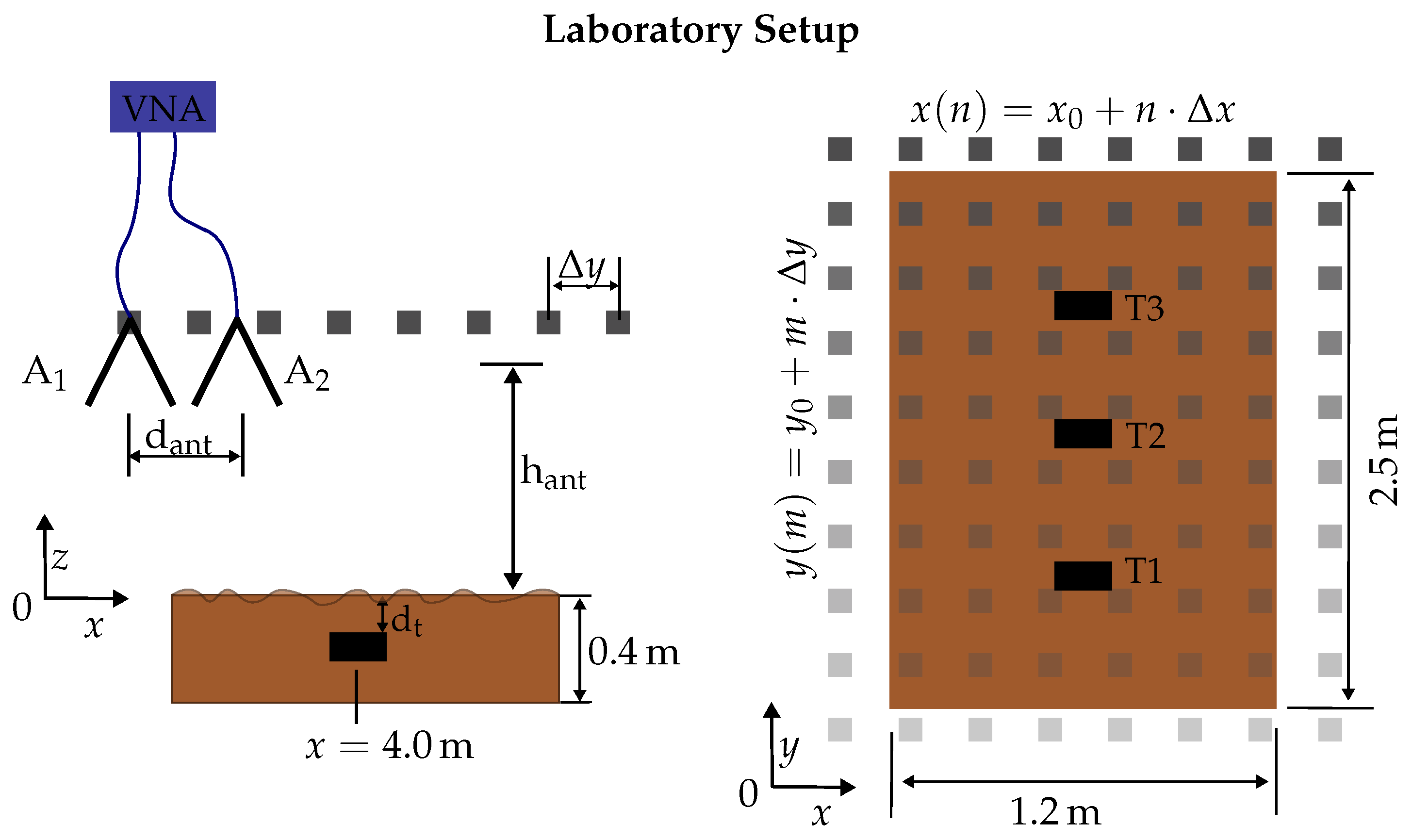
2.5. Laboratory Measurements
2.5.1. Setup
2.5.2. Buried Test Objects
2.5.3. Rough Surface
2.5.4. Vegetation
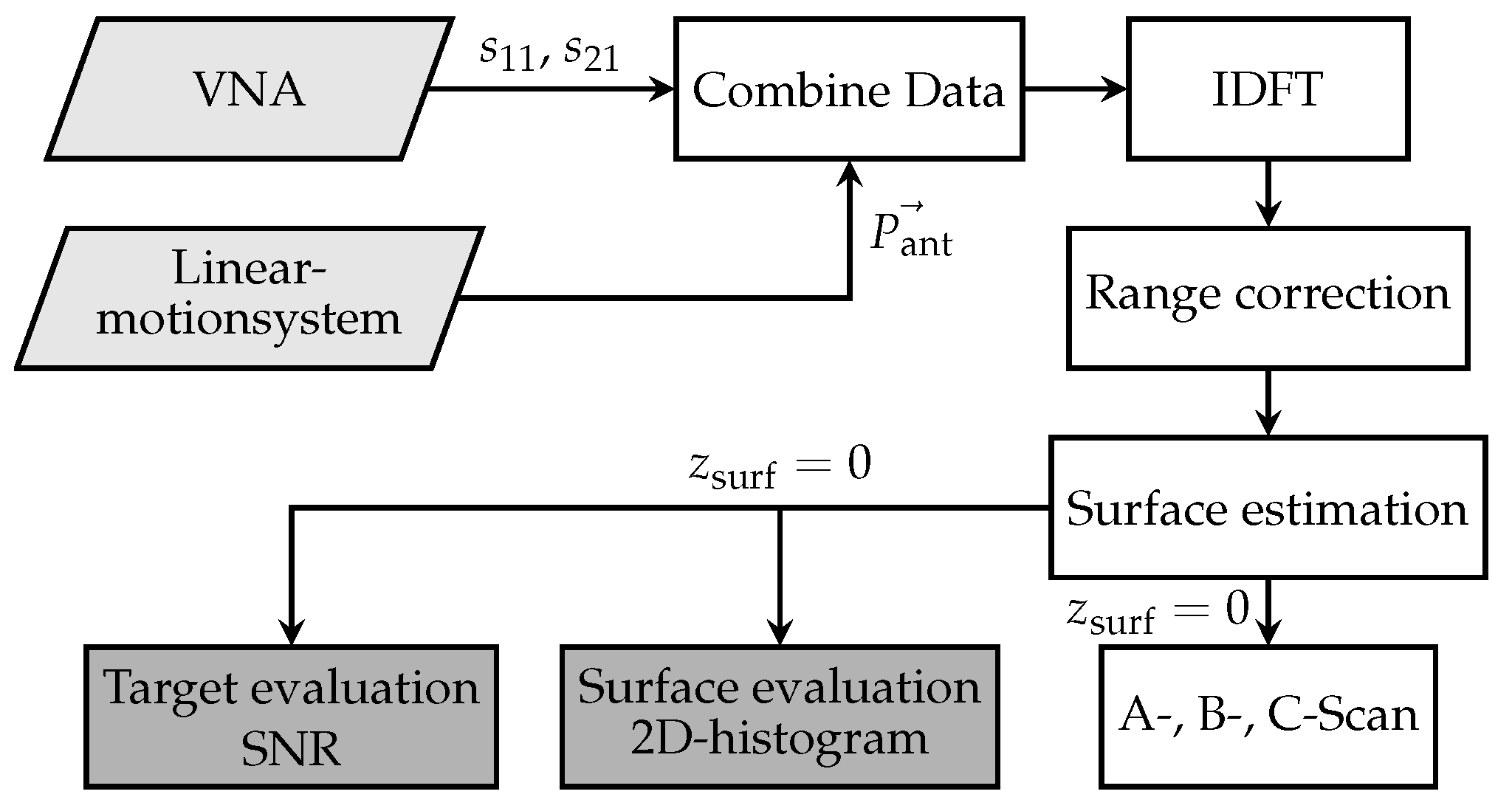
2.6. SFCW GPR Data Processing
2.6.1. Surface Evaluation
2.6.2. Target Evaluation
2.7. Determination of Environmental Parameters
3. Results
 ) at the bottom.
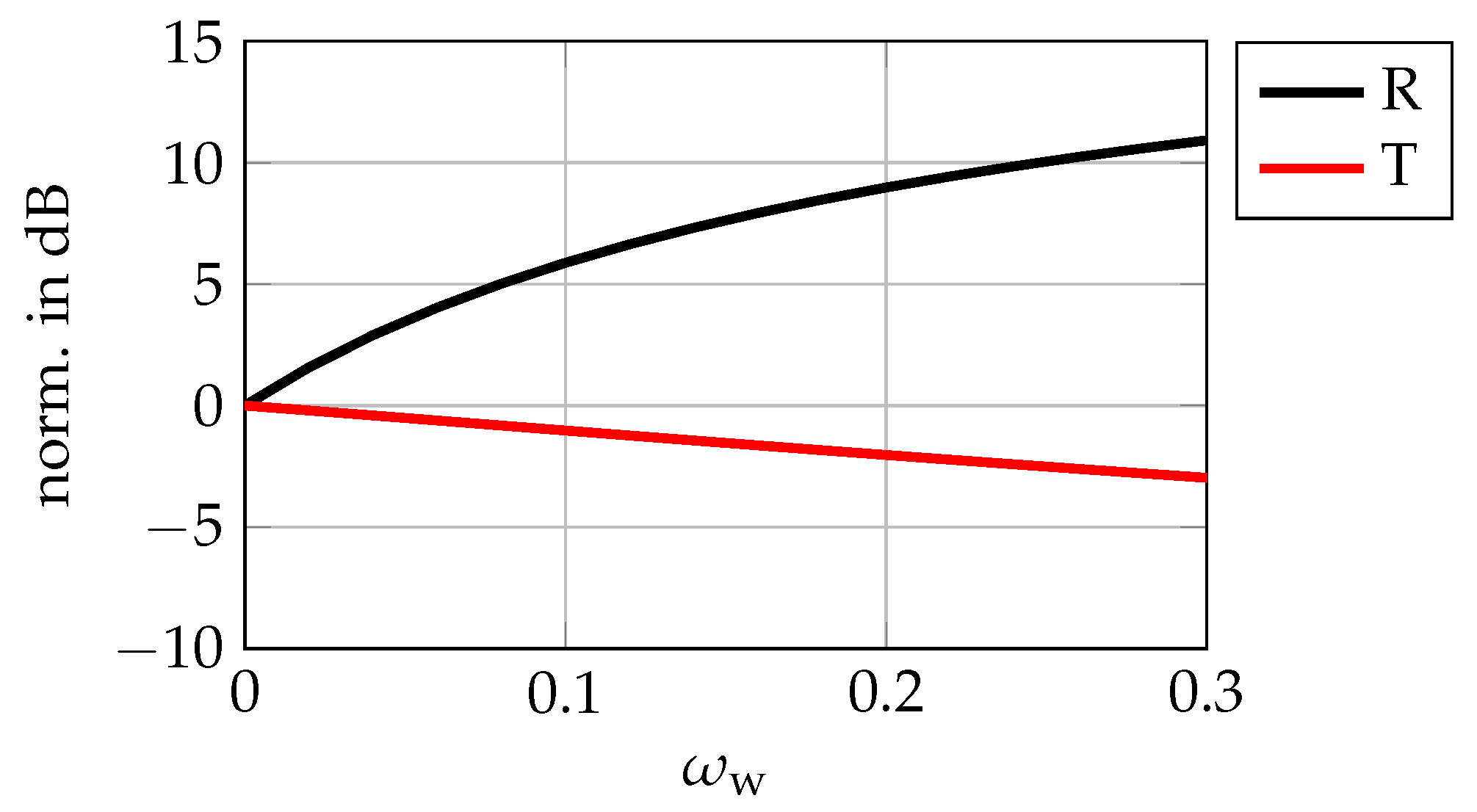
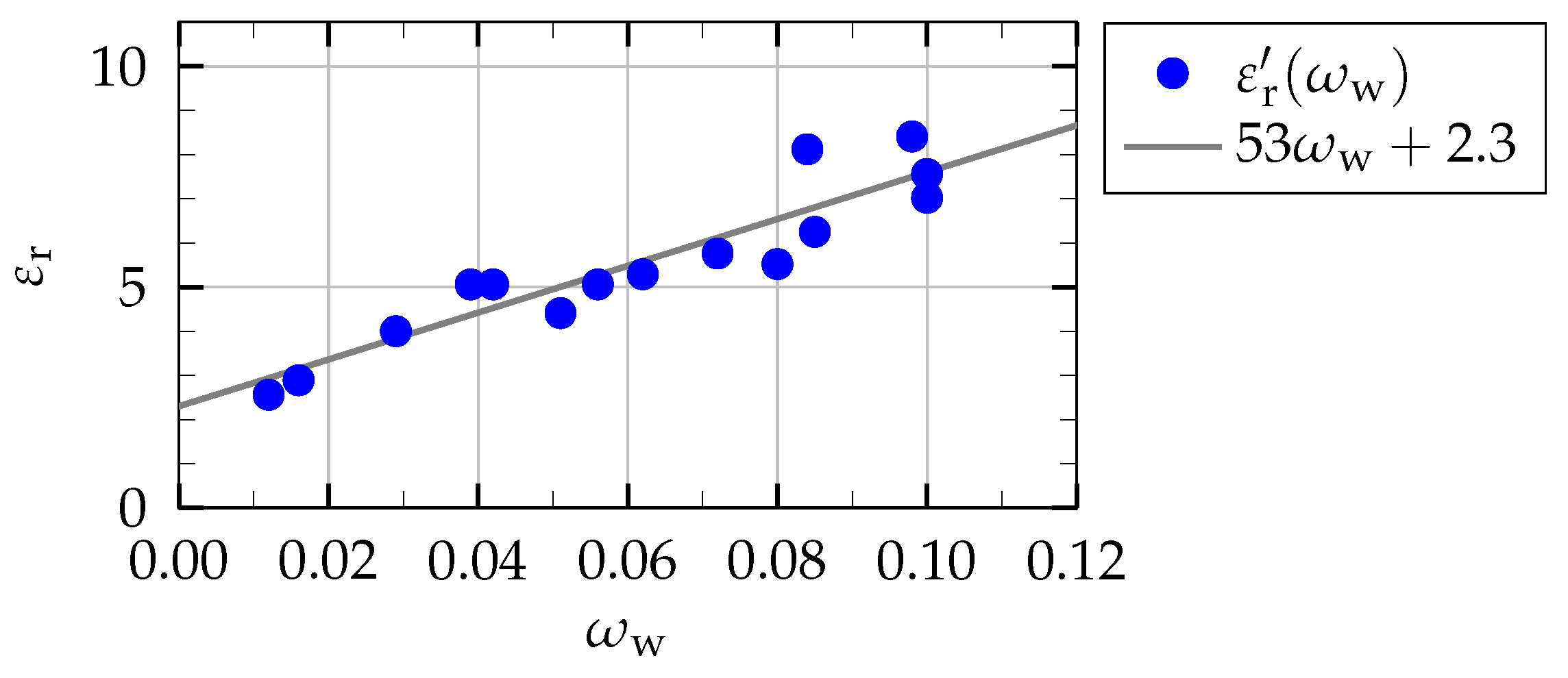
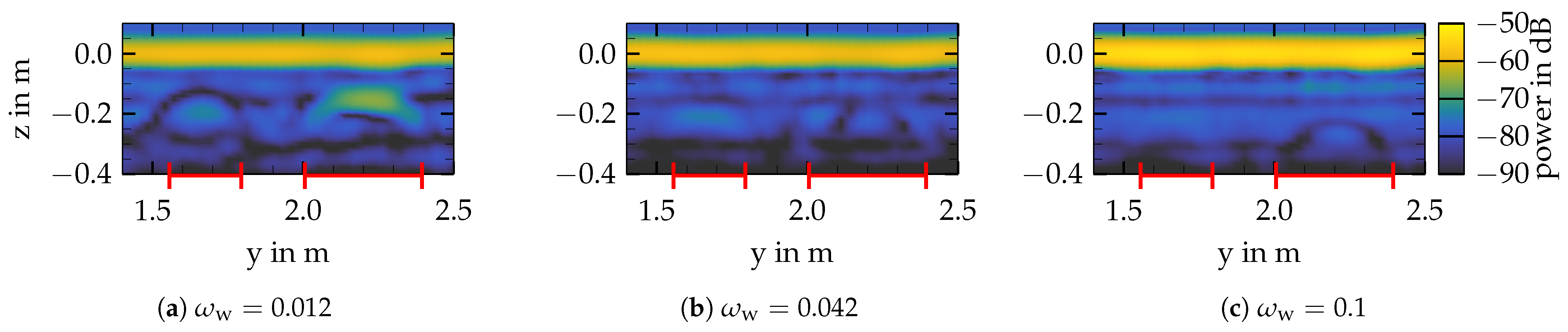
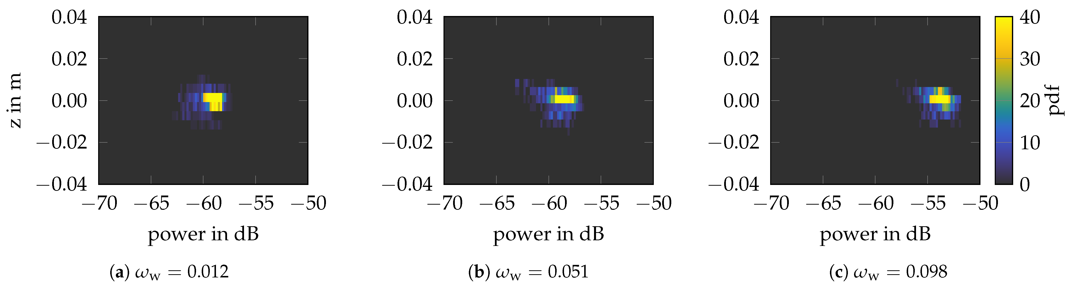
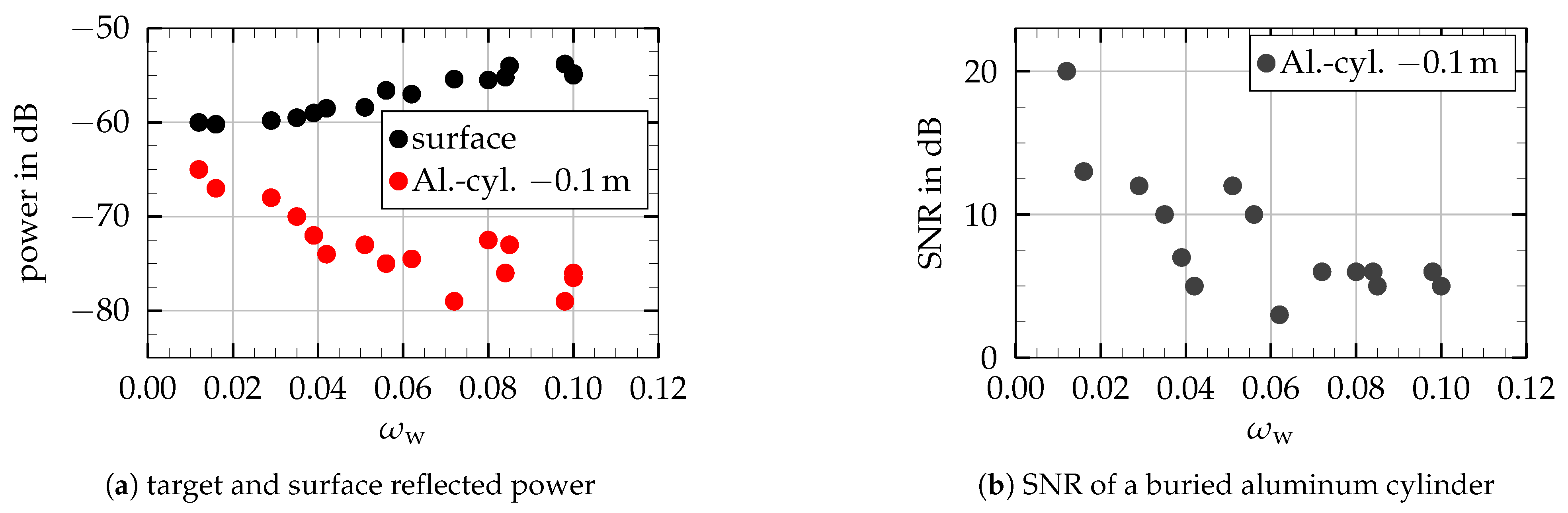
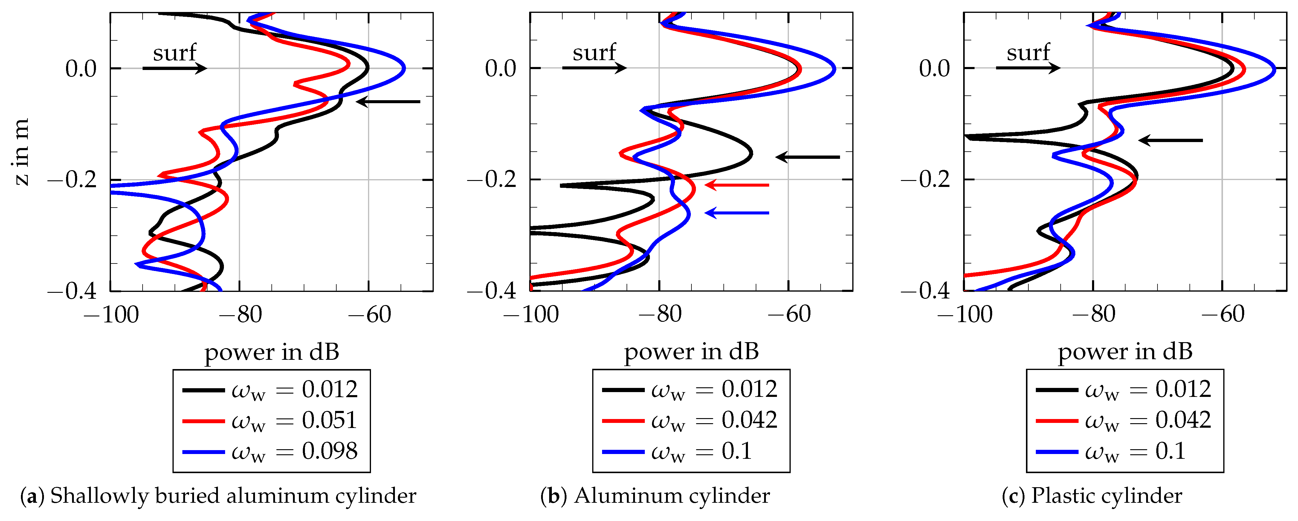
3.1. Influence of the Soil Moisture
Conclusions
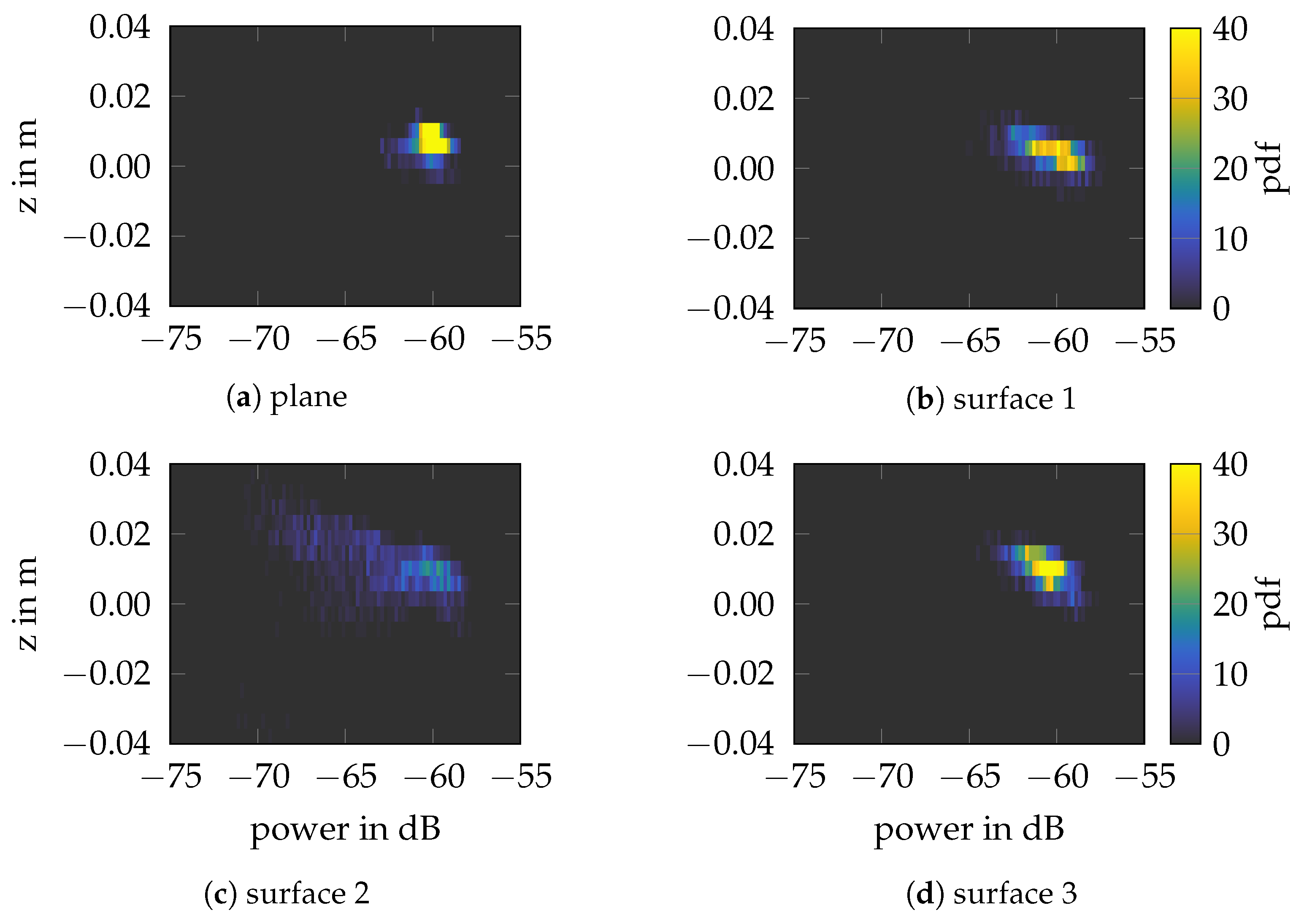
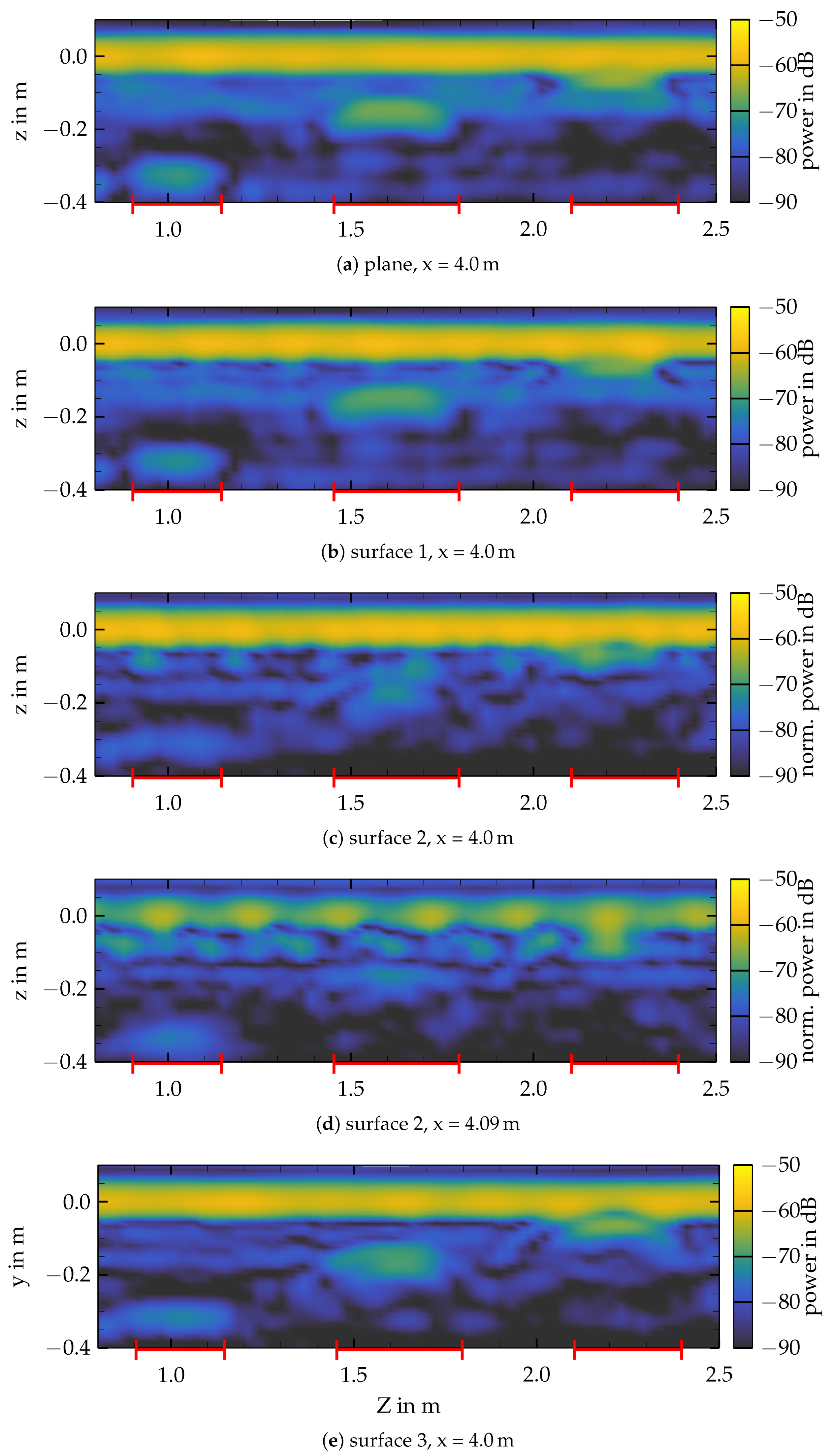
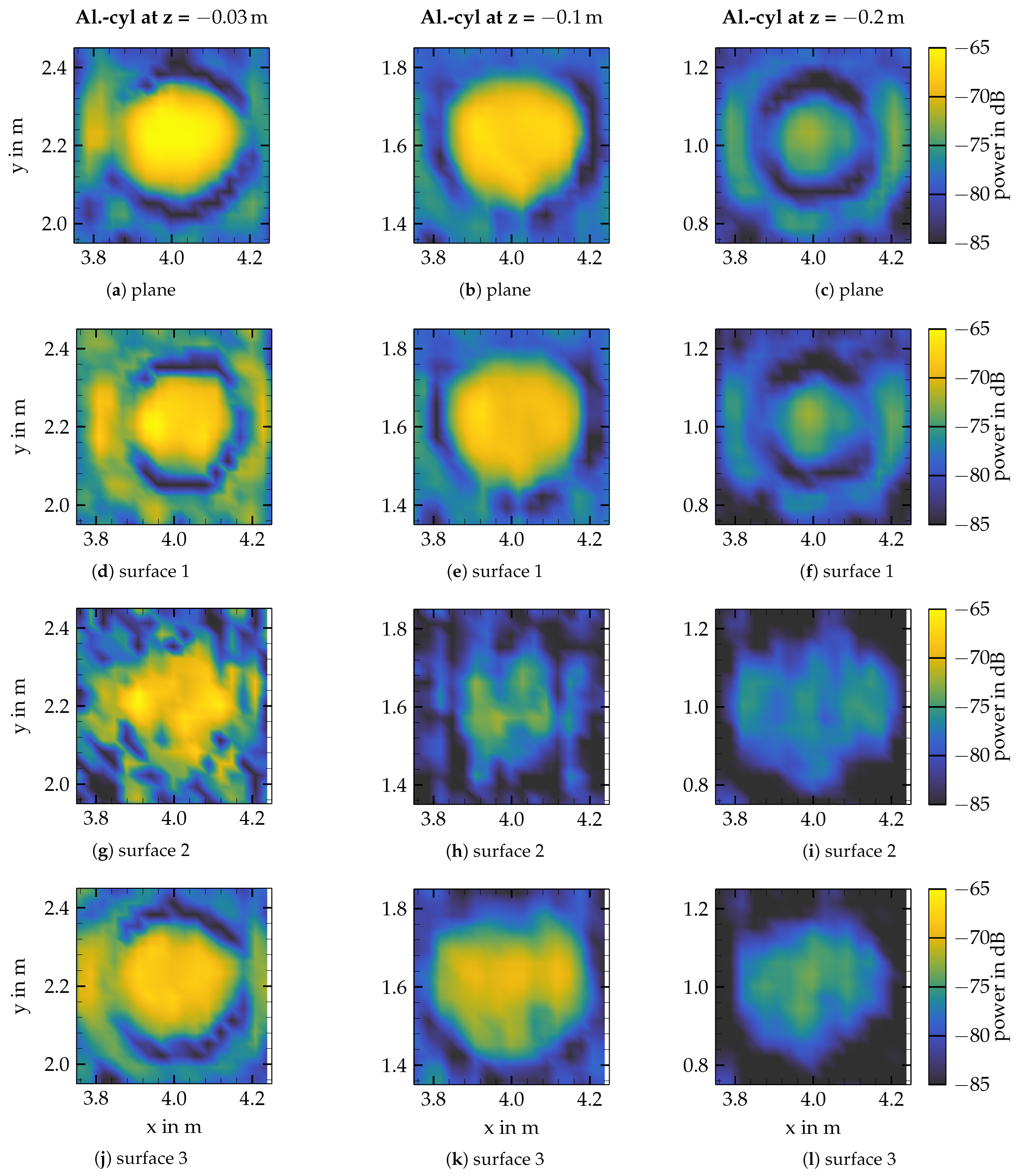
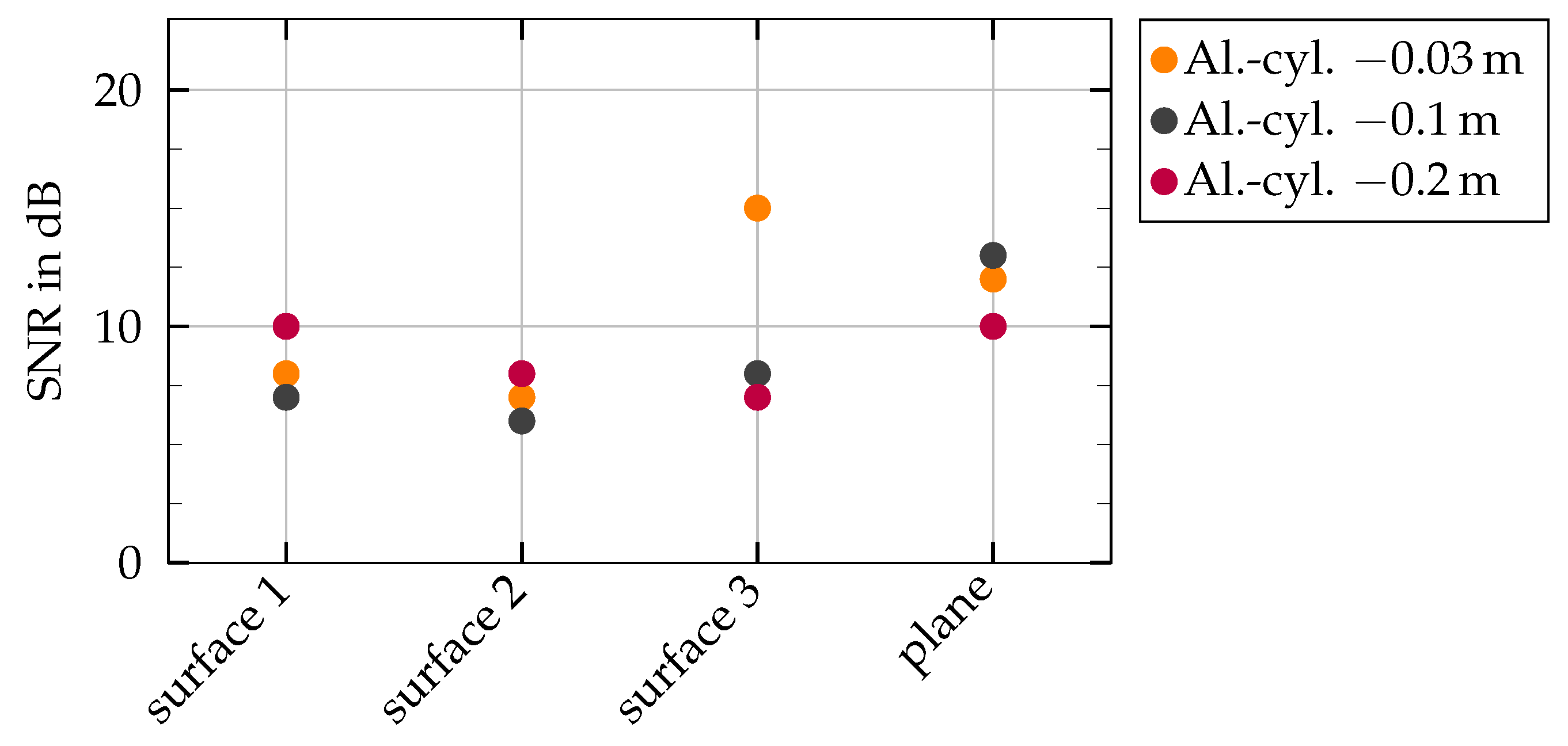
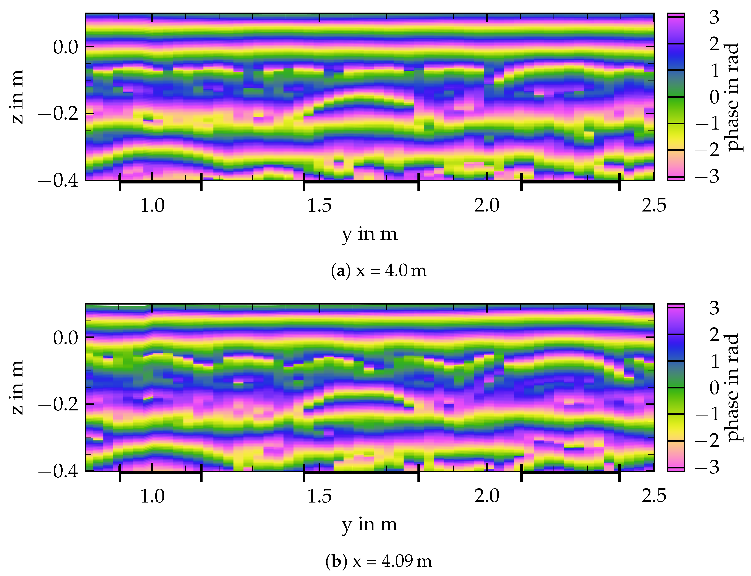
3.2. Surface Roughness
Conclusions
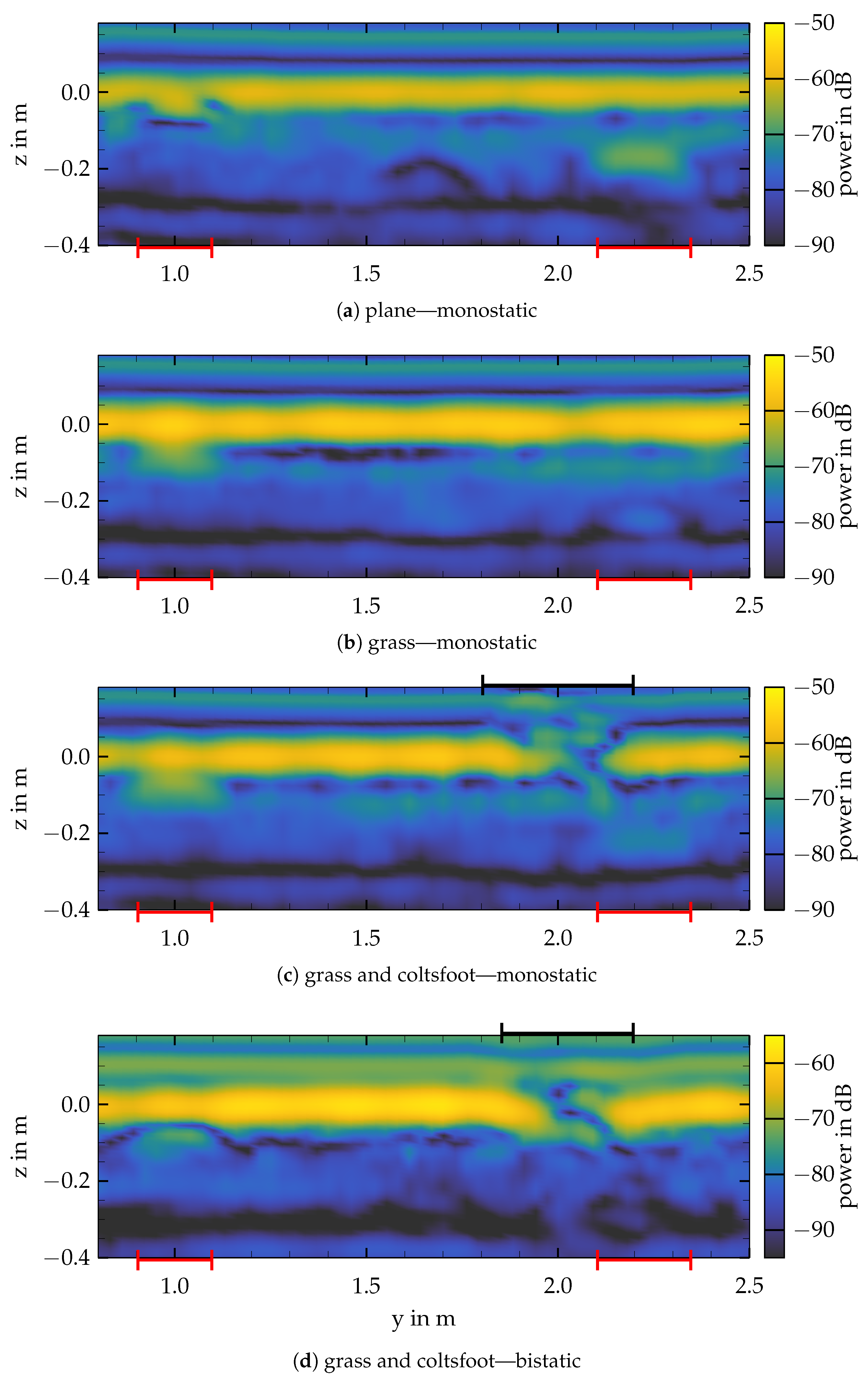
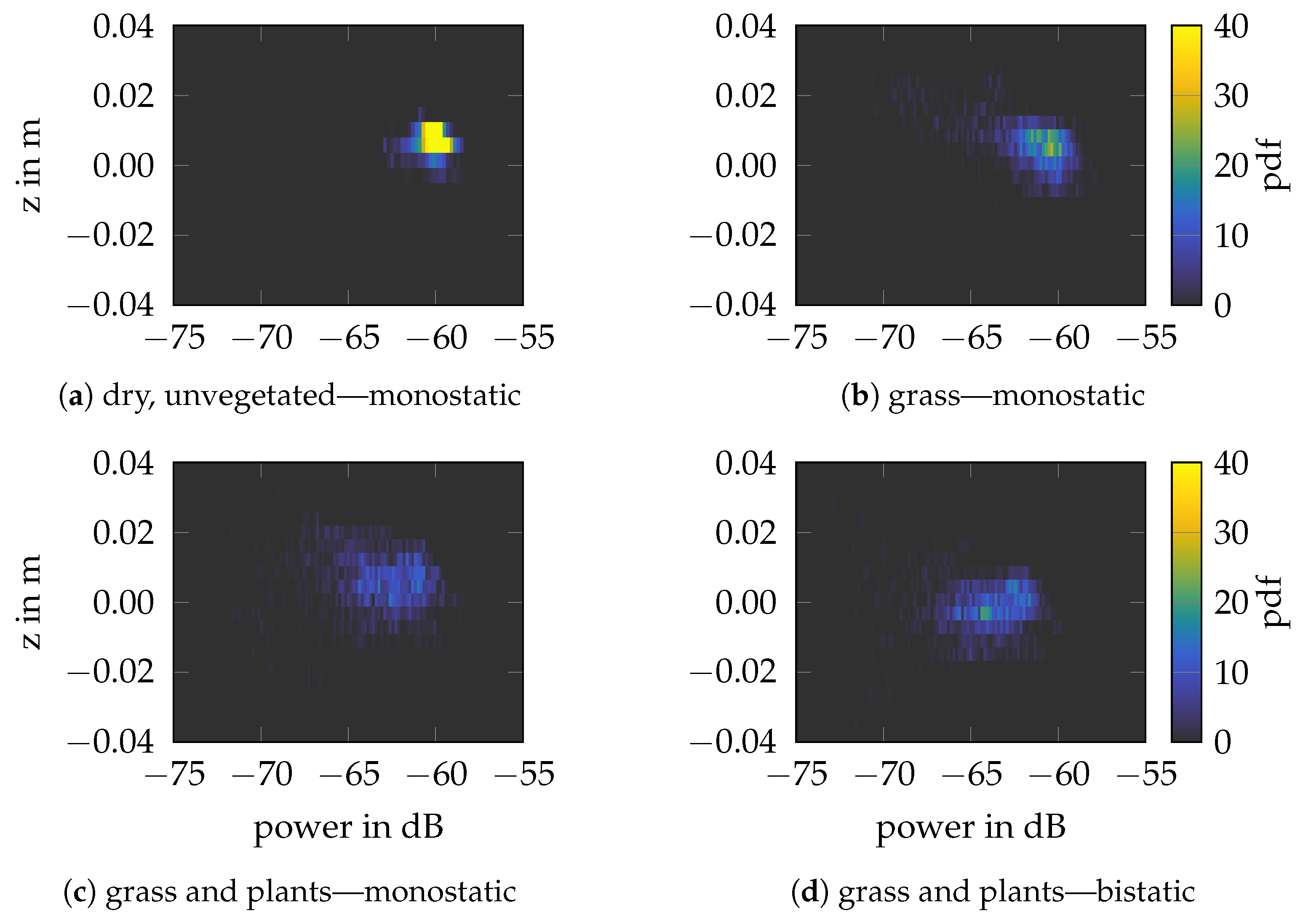
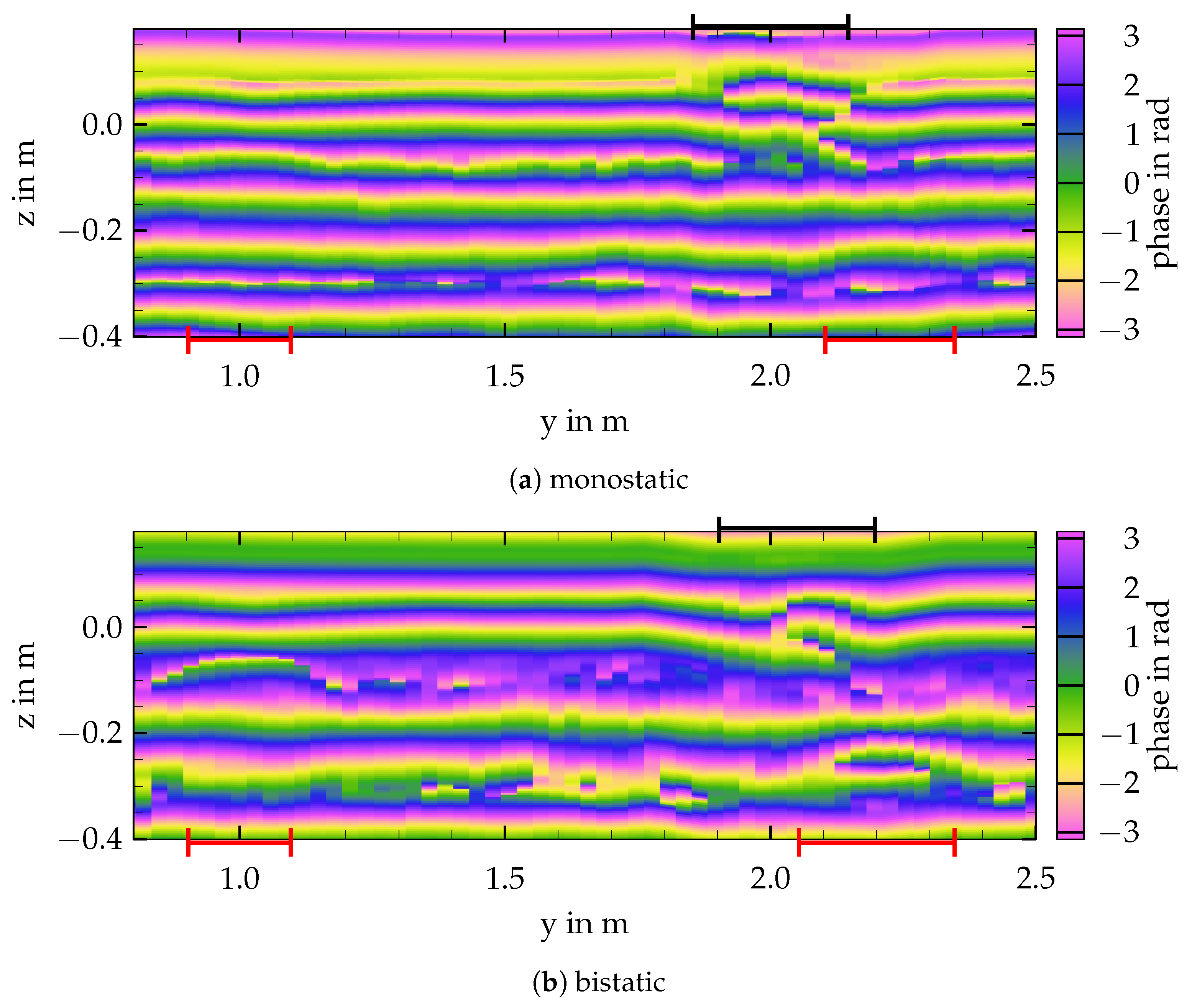
3.3. Vegetation
 ) at the top.
Conclusions
3.4. Comparison of the Various Influences
4. Discussion and Conclusions
- Separation and quantification of environmental impact parameters;
- Identification of critical paths for landmine detection;
- Optimization of data representation for a robust detection.
4.1. Separation of Environmental Impact Parameters
4.2. Identification of Critical Paths for Landmine Detection
4.3. Optimization of Data Representation for a Robust Detection
Author Contributions
Funding
Data Availability Statement
Conflicts of Interest
References
- Sherwin, M. Landmine Monitor 2022: Landmine Monitor 24th Annual Edition; Landmine and Cluster Munition Monitor ICBL-CMC: Geneva, Switzerland, 2022; ISBN 978-2-9701476-2-6. Available online: https://www.the-monitor.org/en-gb/reports/2022/landmine-monitor-2022.aspx (accessed on 15 January 2024).
- Schartel, M.; Burr, R.; Bähnemann, R.; Mayer, W.; Waldschmidt, C. An Experimental Study on Airborne Landmine Detection Using a Circular Synthetic Aperture Radar. arXiv 2020, arXiv:2005.02600. [Google Scholar]
- García-Fernández, M.; Álvarez Narciandi, G.; Álvarez López, Y.; Las-Heras, F. Array-Based Ground Penetrating Synthetic Aperture Radar on Board an Unmanned Aerial Vehicle for Enhanced Buried Threats Detection. IEEE Trans. Geosci. Remote Sens. 2023, 61, 5104218. [Google Scholar] [CrossRef]
- Garcia-Fernandez, M.; Alvarez-Narciandi, G.; Lopez, Y.A.; Andres, F.L.H. SAFEDRONE project: Development of a UAV-based high-resolution GPR system for IED detection. In Proceedings of the 2022 16th European Conference on Antennas and Propagation (EuCAP), Madrid, Spain, 27 March–1 April 2022. [Google Scholar] [CrossRef]
- Kondo, T.; Kikuta, K.; Sato, M. Ground Surface Reflection Compensation for Hand-Held GPR. IEEE Geosci. Remote Sens. Lett. 2022, 19, 3501605. [Google Scholar] [CrossRef]
- Vallon. Vallon VMR3G Minehound-Dual-Sensor-Detektor; Vallon GmbH: Eningen, Germany, 2024; Available online: https://vallon-dual-sensor-detectors.com/de/ (accessed on 5 January 2024).
- Romero, I.; Walter, T.; Mariager, S. Wavelet Transform Analysis for a Continuous Wave Metal Detector for UAV Applications. In Proceedings of the IGARSS 2023—2023 IEEE International Geoscience and Remote Sensing Symposium, Pasadena, CA, USA, 16–21 July 2023. [Google Scholar] [CrossRef]
- García-Fernández, M.; López, Y.A.; Andrés, F.L.H. Airborne Multi-Channel Ground Penetrating Radar for Improvised Explosive Devices and Landmine Detection. IEEE Access 2020, 8, 165927–165943. [Google Scholar] [CrossRef]
- Grathwohl, A.; Arendt, B.; Grebner, T.; Waldschmidt, C. Detection of Objects Below Uneven Surfaces With a UAV-Based GPSAR. IEEE Trans. Geosci. Remote Sens. 2023, 61, 5207913. [Google Scholar] [CrossRef]
- Debye, P.J.W. Polar Molecules; The Chemical Catalog Company, Inc.: New York, NY, USA, 1929. [Google Scholar]
- Said, T.; Varadan, V.V. Variation of Cole-Cole model parameters with the complex permittivity of biological tissues. In Proceedings of the 2009 IEEE MTT-S International Microwave Symposium Digest, Boston, MA, USA, 7–12 June 2009. [Google Scholar] [CrossRef]
- Bobrov, P.P.; Kroshka, E.S.; Lapina, A.S.; Repin, A.V. Relaxation model of complex relative permittivity of sandstones for the frequency range from 10 kHz to 1 GHz. In Proceedings of the 2017 Progress In Electromagnetics Research Symposium—Spring (PIERS), St. Petersburg, Russia, 22–25 May 2017. [Google Scholar] [CrossRef]
- Peplinski, N.; Ulaby, F.; Dobson, M. Dielectric properties of soils in the 0.3–1.3-GHz range. IEEE Trans. Geosci. Remote Sens. 1995, 33, 803–807. [Google Scholar] [CrossRef]
- Topp, G.C.; Davis, J.L.; Annan, A.P. Electromagnetic determination of soil water content: Measurements in coaxial transmission lines. Water Resour. Res. 1980, 16, 574–582. [Google Scholar] [CrossRef]
- Scharf, P.A.; Iberle, J.; Mantz, H.; Walter, T.; Waldschmidt, C. Multiband Microwave Sensing for Surface Roughness Classification. In Proceedings of the 2018 IEEE/MTT-S International Microwave Symposium–IMS, Philadelphia, PA, USA, 10–15 June 2018. [Google Scholar] [CrossRef]
- Tan, H.S. Microwave measurements and modelling of the permittivity of tropical vegetation samples. Appl. Phys. 1981, 25, 351–355. [Google Scholar] [CrossRef]
- Mahmoudzadeh Ardekani, M.R.; Jacques, D.C.; Lambot, S. A Layered Vegetation Model for GPR Full-Wave Inversion. IEEE J. Sel. Top. Appl. Earth Obs. Remote Sens. 2016, 9, 18–28. [Google Scholar] [CrossRef]
- Wehner, D.R. High Resolution Radar, 2nd ed.; Artech House Radar Library, Artech House: Norwood, MA, USA, 1995. [Google Scholar]
- Davis, J.L.; Annan, A.P. Ground-Penetrating Radar for high-resolution mapping of soil and rock stratigraphy. Geophys. Prospect. 1989, 37, 531–551. [Google Scholar] [CrossRef]
- Turk, A.S. Subsurface Sensing, 1st ed.; Wiley Series in Microwave and Optical Engineering Ser; John Wiley & Sons Incorporated: Hoboken, NJ, USA, 2011; Volume 197. [Google Scholar]
- Warren, C.; Giannopoulos, A.; Giannakis, I. gprMax: Open source software to simulate electromagnetic wave propagation for Ground Penetrating Radar. Comput. Phys. Commun. 2016, 209, 163–170. [Google Scholar] [CrossRef]
- Perdok, U.; Kroesbergen, B.; Hilhorst, M. Influence of gravimetric water content and bulk density on the dielectric properties of soil. Eur. J. Soil Sci. 1996, 47, 367–371. [Google Scholar] [CrossRef]
- Roth, K.; Schulin, R.; Flühler, H.; Attinger, W. Calibration of time domain reflectometry for water content measurement using a composite dielectric approach. Water Resour. Res. 1990, 26, 2267–2273. [Google Scholar] [CrossRef]
- Arendt, B.; Grathwohl, A.; Waldschmidt, C.; Walter, T. Influence of Vegetation on the Detection of Shallowly Buried Objects with a UAV-Based GPSAR. In Proceedings of the IGARSS 2022—2022 IEEE International Geoscience and Remote Sensing Symposium, Kuala Lumpur, Malaysia, 17–22 July 2022. [Google Scholar] [CrossRef]
- Geng, N.; Wiesbeck, W. Planungsmethoden für die Mobilkommunikation; 1., softcover reprint of the original 1st ed. 1998 ed.; Information und Kommunikation; Springer: Berlin, Germany, 2013. [Google Scholar]
- Thomas, T.R. Rough Surfaces; Published by Imperial College Press and Distributed by World Scientific Publishing Co.: London, UK, 1998. [Google Scholar] [CrossRef]
- Bergström, D.; Powell, J.; Kaplan, A.F. The absorption of light by rough metal surfaces—A three-dimensional ray-tracing analysis. J. Appl. Phys. 2008, 103, 103515. [Google Scholar] [CrossRef]
- Tsang, L.; Kong, J.A.; Ding, K. Scattering of Electromagnetic Waves: Theories and Applications; Wiley: New York, NY, USA, 2000. [Google Scholar] [CrossRef]
- Keysight. Network Analyzer FieldFox Handheld RF; Keysight: Santa Rosa, CA, USA, 2023; Available online: https://www.keysight.com/us/en/products/network-analyzers/fieldfox-handheld-rf-microwave-analyzers.html (accessed on 8 January 2024).
- Aaronia. AARONIA PowerLOG® 70180 Hornantenna; Aaronia AG: Euscheid, Germany, 2023; Available online: https://aaronia.com/de/shop/antennen-sensoren/horn-antennas/horn-antenna (accessed on 20 January 2024).
- Harris, F. On the use of windows for harmonic analysis with the discrete Fourier transform. Proc. IEEE 1978, 66, 51–83. [Google Scholar] [CrossRef]
- Adams, J. A new optimal window (signal processing). IEEE Trans. Signal Process. 1991, 39, 1753–1769. [Google Scholar] [CrossRef]
- Yelf, R. Where is true time zero? In Proceedings of the Tenth International Conference on Ground Penetrating Radar, Delft, The Netherlands, 21–24 June 2004; GPR 2004. Univ. of Technology: Delft, The Netherlands, 2004. [Google Scholar]
- Ulaby, F.T.; Moore, R.K.; Fung, A.K. Radar Remote Sensing and Surface Scattering and Emission Theory; Artech House: Norwood, MA, USA, 1986; Volume 2. [Google Scholar]


| Environmental Factor | Influence | Model | Comment |
|---|---|---|---|
| water | frequency dependence | Debye Model [10] Cole–Cole model [11,12] | basic theory |
| soil parameters 2 | frequency dependence attenuation reflection R, transmission T | Peplinski soil model [13] CRIM 1 Topp equation [14] | semi-empirical model for mixed-media empirical model |
| surface roughness | scattering of EM-waves | Fresnel–Kirchhoff Diffraction [15] | key parameter: |
| vegetation 2 | frequency dependence scattering of EM-waves attenuation | Tan formulation [16] CRIM 1 for homogeneous layer [17] | 3D structure/shape not considered |
| Parameter | Surface 1 | Surface 2 | Surface 3 |
|---|---|---|---|
| edge length | 0.25 m | 0.25 m | 0.25 m |
| ℓ | 26.25 mm | 26.25 mm | 13.125 mm |
| 3.75 mm | 7.5 mm | 3.75 mm | |
| 0.202 | 0.404 | 0.404 |
| Parameter | Value | Comment |
|---|---|---|
| VNA Frequency Range | 0.8 GHz–5 GHz | 1001 points |
| width of range bin | 4.4 mm | zero padding of 8 |
| Antenna Bandwidth | 0.7 GHz to 18 GHz | Double Ridge Horn [30] |
| Antenna Beamwidth | ≈80° to 30° | - |
| , | 0.03 m | - |
| hant | 0.3 m | - |
| dant | 0.28 m | - |
| soil type | loamy sand | - |
| Wavelength | Rayleigh Criterion | Fraunhofer Criterion |
|---|---|---|
| 0.37 m | 46.25 mm | 11.56 mm |
| 0.10 m | 12.87 mm | 3.22 mm |
| 0.06 m | 7.5 mm | 1.87 mm |
| Parameter | Formula | Unit | Comment |
|---|---|---|---|
| gravimetric soil moisture content | ISO 11465 dryed at 110 °C | ||
| surface roughness | parameters Table 2, criteria in Table 4 | molds are synthetically generated | |
| vegtation mass per area | - | ||
| gravimetric vegetation moisture content | dryed at 110 °C | ||
| vegetation height | - | ||
| vegetation structure | - | different for each plant species |
Disclaimer/Publisher’s Note: The statements, opinions and data contained in all publications are solely those of the individual author(s) and contributor(s) and not of MDPI and/or the editor(s). MDPI and/or the editor(s) disclaim responsibility for any injury to people or property resulting from any ideas, methods, instructions or products referred to in the content. |
© 2024 by the authors. Licensee MDPI, Basel, Switzerland. This article is an open access article distributed under the terms and conditions of the Creative Commons Attribution (CC BY) license (https://creativecommons.org/licenses/by/4.0/).
Share and Cite
Arendt, B.; Schneider, M.; Mayer, W.; Walter, T. Environmental Influences on the Detection of Buried Objects with a Ground-Penetrating Radar. Remote Sens. 2024, 16, 1011. https://doi.org/10.3390/rs16061011
Arendt B, Schneider M, Mayer W, Walter T. Environmental Influences on the Detection of Buried Objects with a Ground-Penetrating Radar. Remote Sensing. 2024; 16(6):1011. https://doi.org/10.3390/rs16061011
Chicago/Turabian StyleArendt, Bernd, Michael Schneider, Winfried Mayer, and Thomas Walter. 2024. "Environmental Influences on the Detection of Buried Objects with a Ground-Penetrating Radar" Remote Sensing 16, no. 6: 1011. https://doi.org/10.3390/rs16061011
APA StyleArendt, B., Schneider, M., Mayer, W., & Walter, T. (2024). Environmental Influences on the Detection of Buried Objects with a Ground-Penetrating Radar. Remote Sensing, 16(6), 1011. https://doi.org/10.3390/rs16061011