
Estimating the CSLE Biological Conservation Measures’ B-Factor Using Google Earth’s Engine


Abstract
1. Introduction
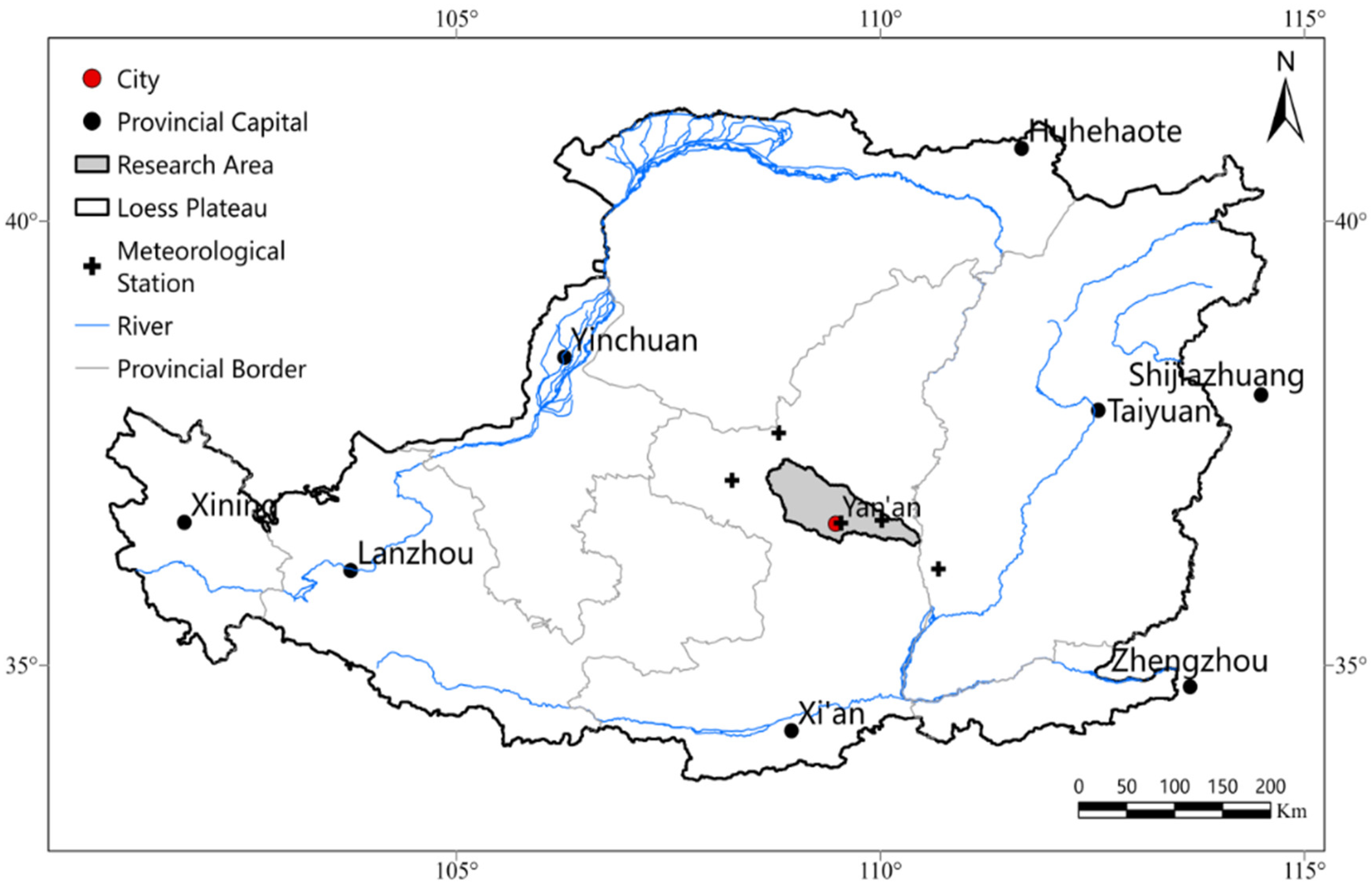
2. The Study Area
3. Materials and Methods
3.1. Data Sources
3.1.1. Rainfall Data
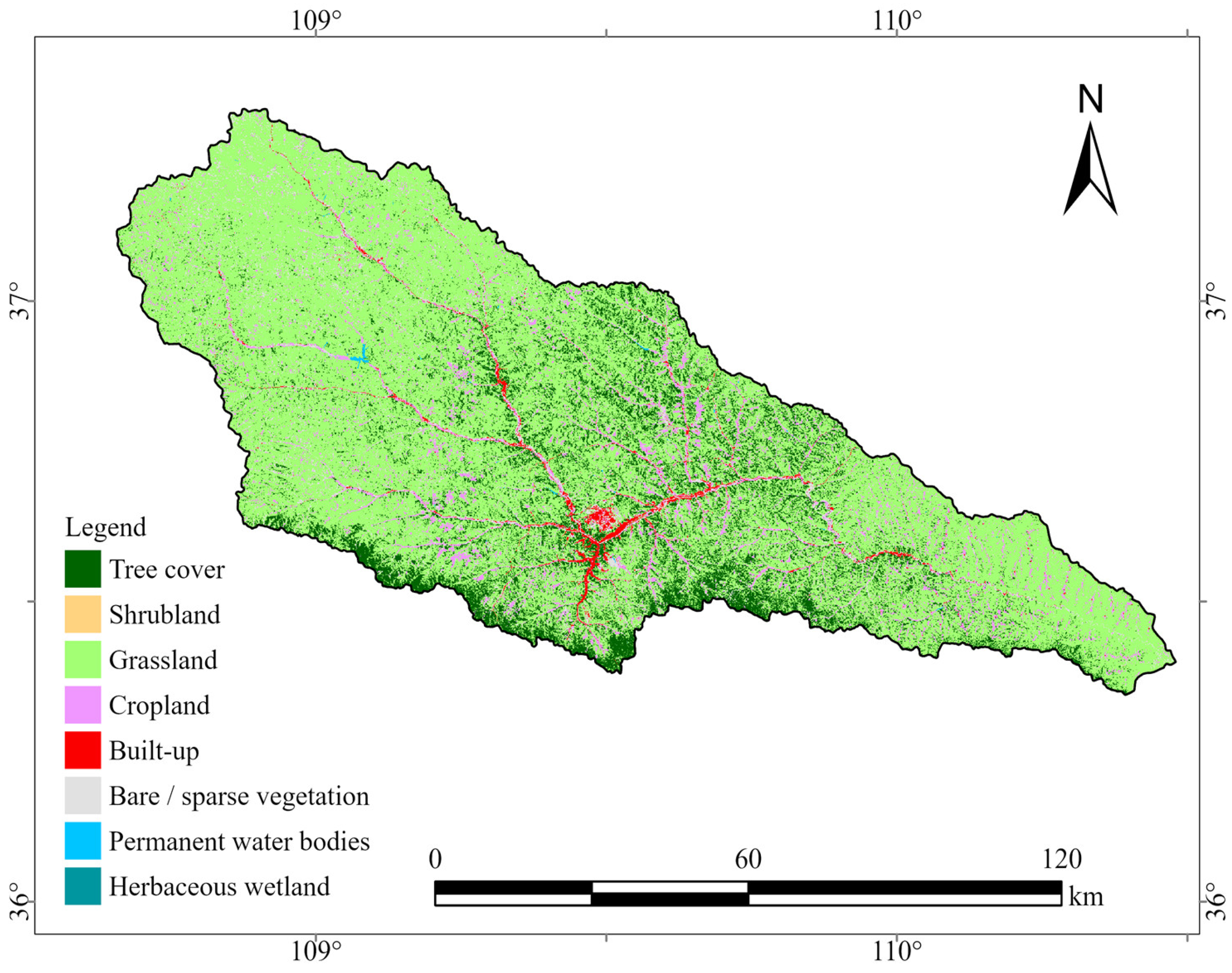
3.1.2. Land Use Data
3.1.3. Remote Sensing Data
3.2. Technological Procedure
- (1)
- The applicability of three gridded daily precipitation datasets CHIRPS, ERA5, and PERSIANN-CDR in the GEE for the Yan River Basin was assessed against the data from national meteorological stations. The dataset that demonstrated the highest suitability was chosen to calculate rainfall erosivity and its proportion.
- (2)
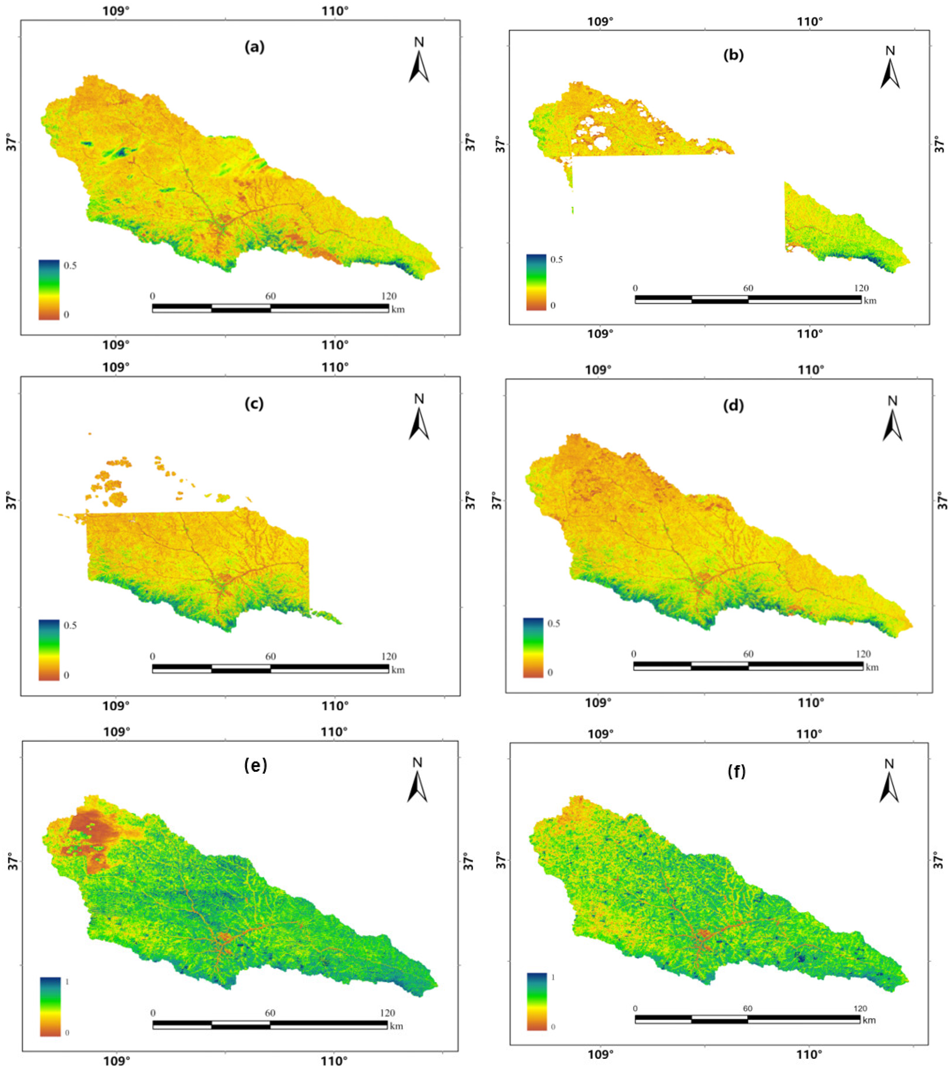
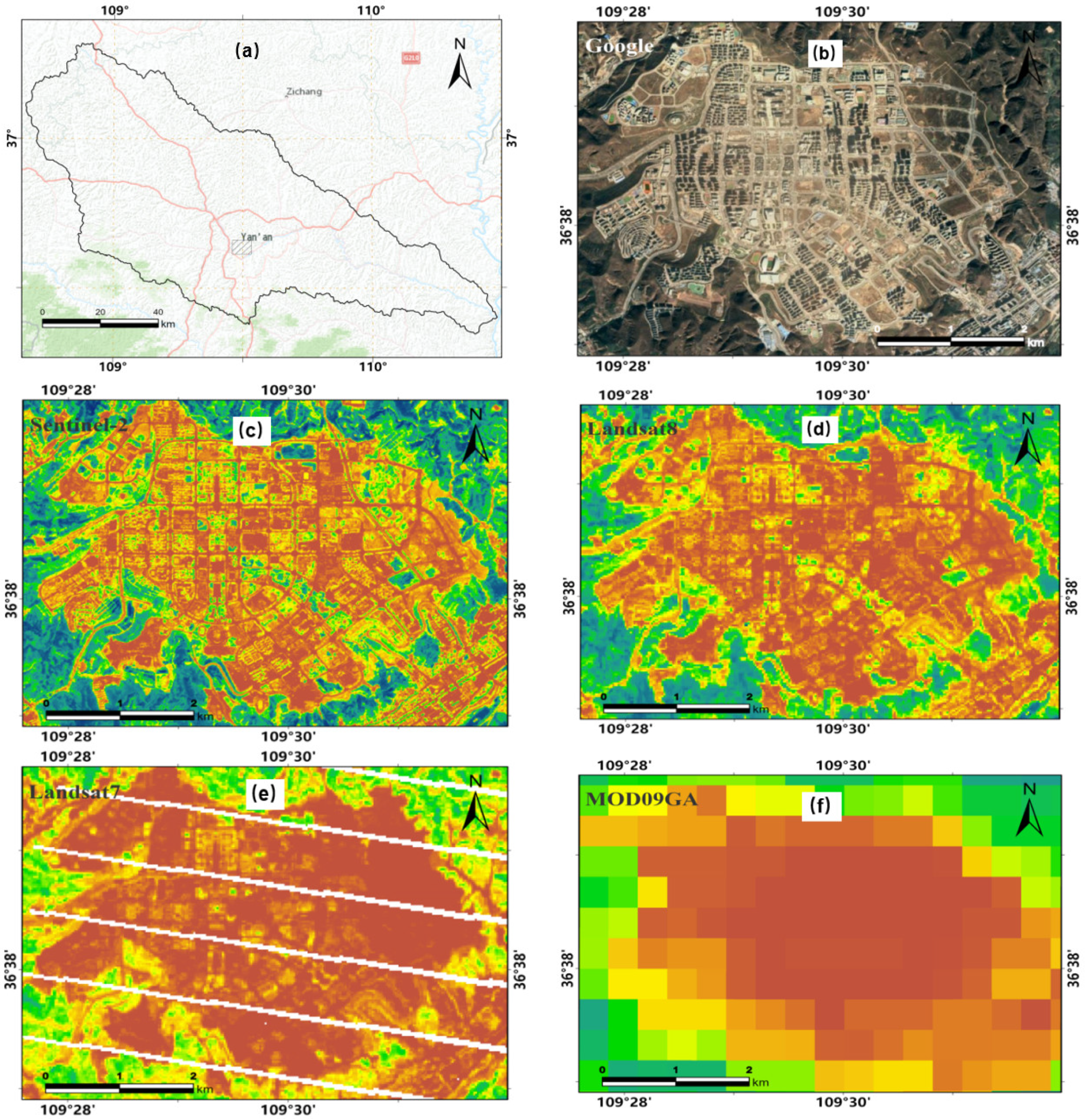
- MOD09GA, Sentinel-2, Landsat 8, and Landsat imagery data were obtained and preprocessed, and the missing areas in the Sentinel-2 data were then identified.
- (3)
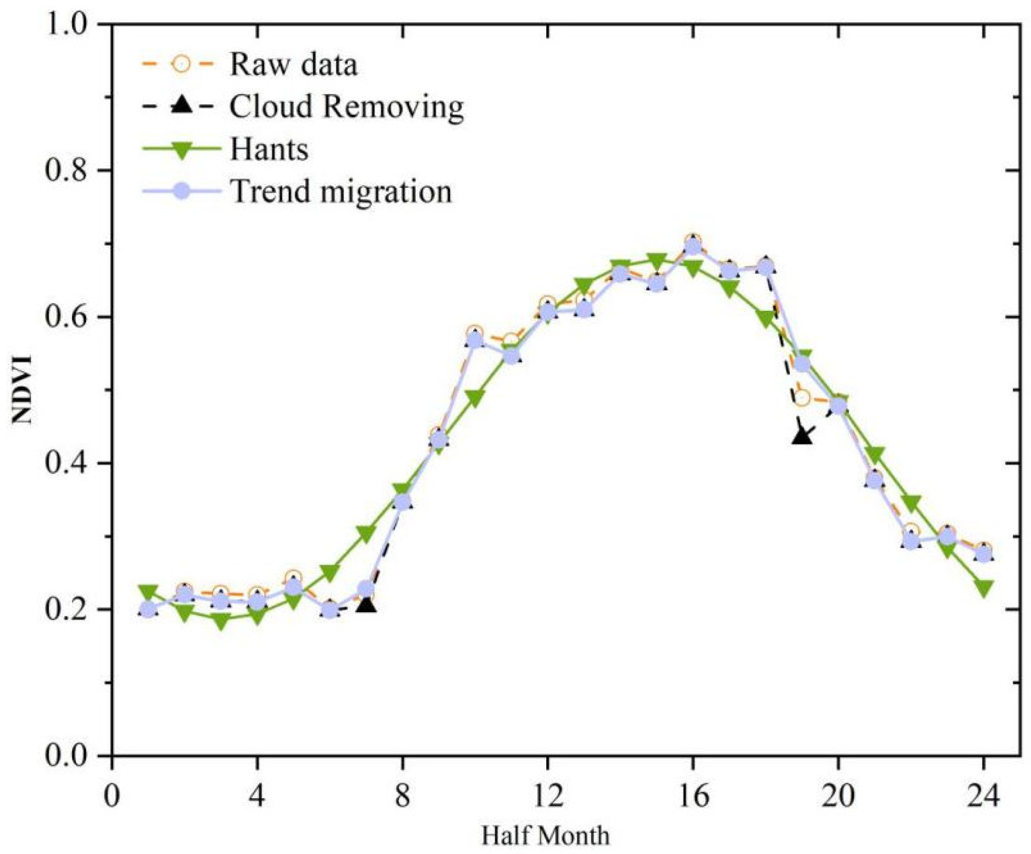
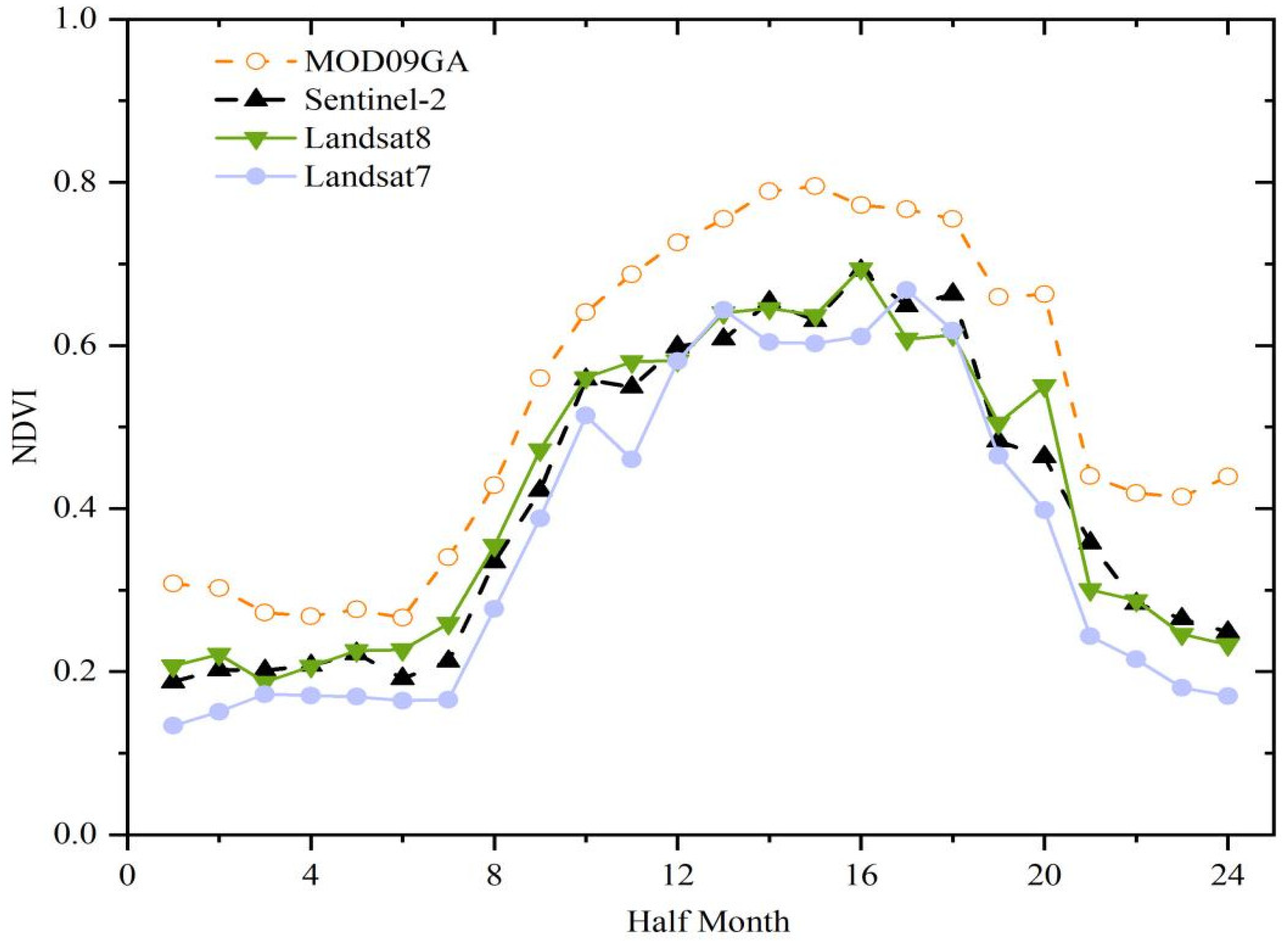
- The normalized difference vegetation index (NDVI) was computed separately for each of these four datasets. The missing NDVI data in Sentinel-2 were patched using NDVI calculated from MOD09GA, Landsat 8, and Landsat 7.
- (4)
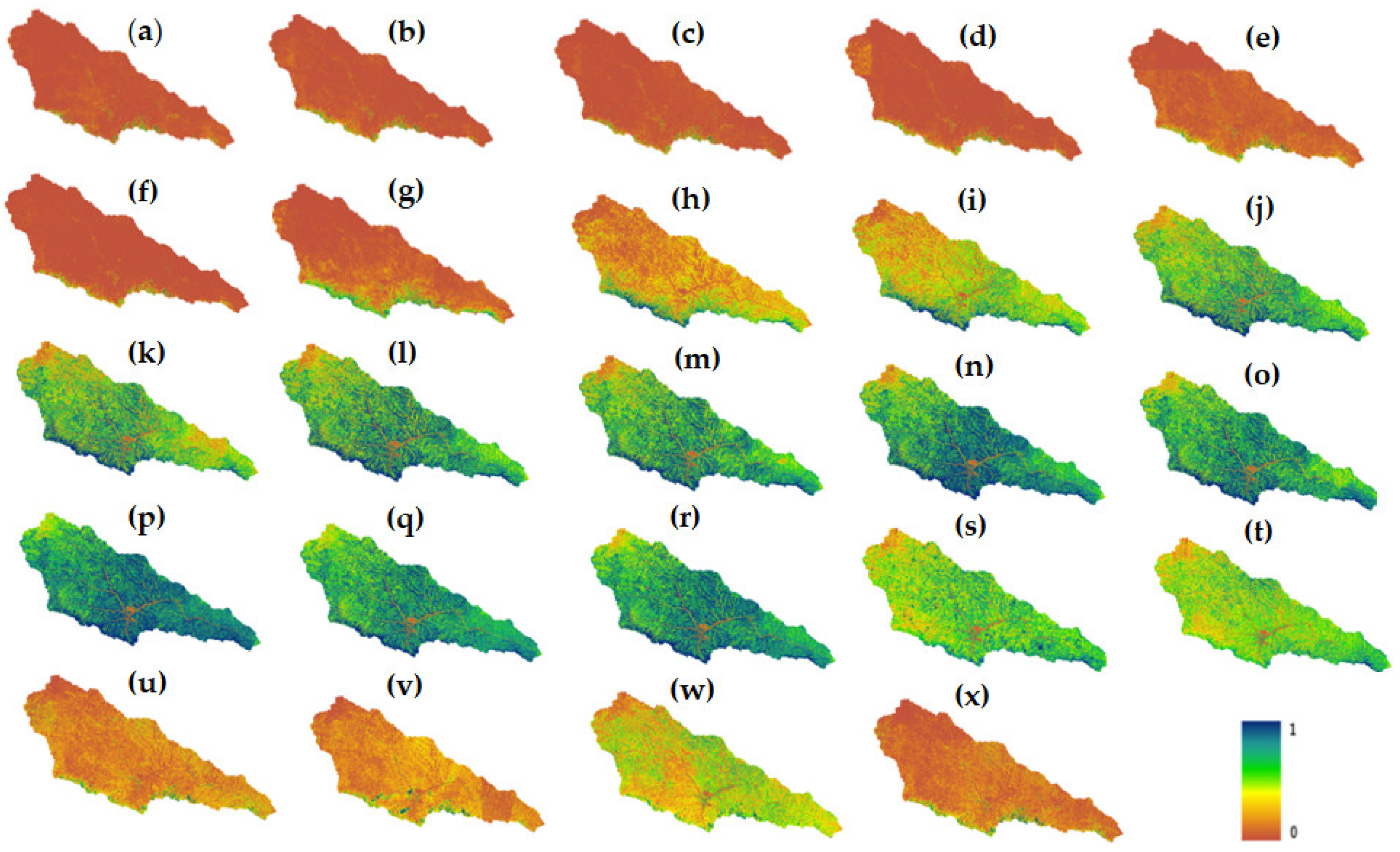
- The patched NDVI data were analyzed using the pixel binary method to determine the average vegetation coverage (FVC) for 24 half-months over three years.
- (5)
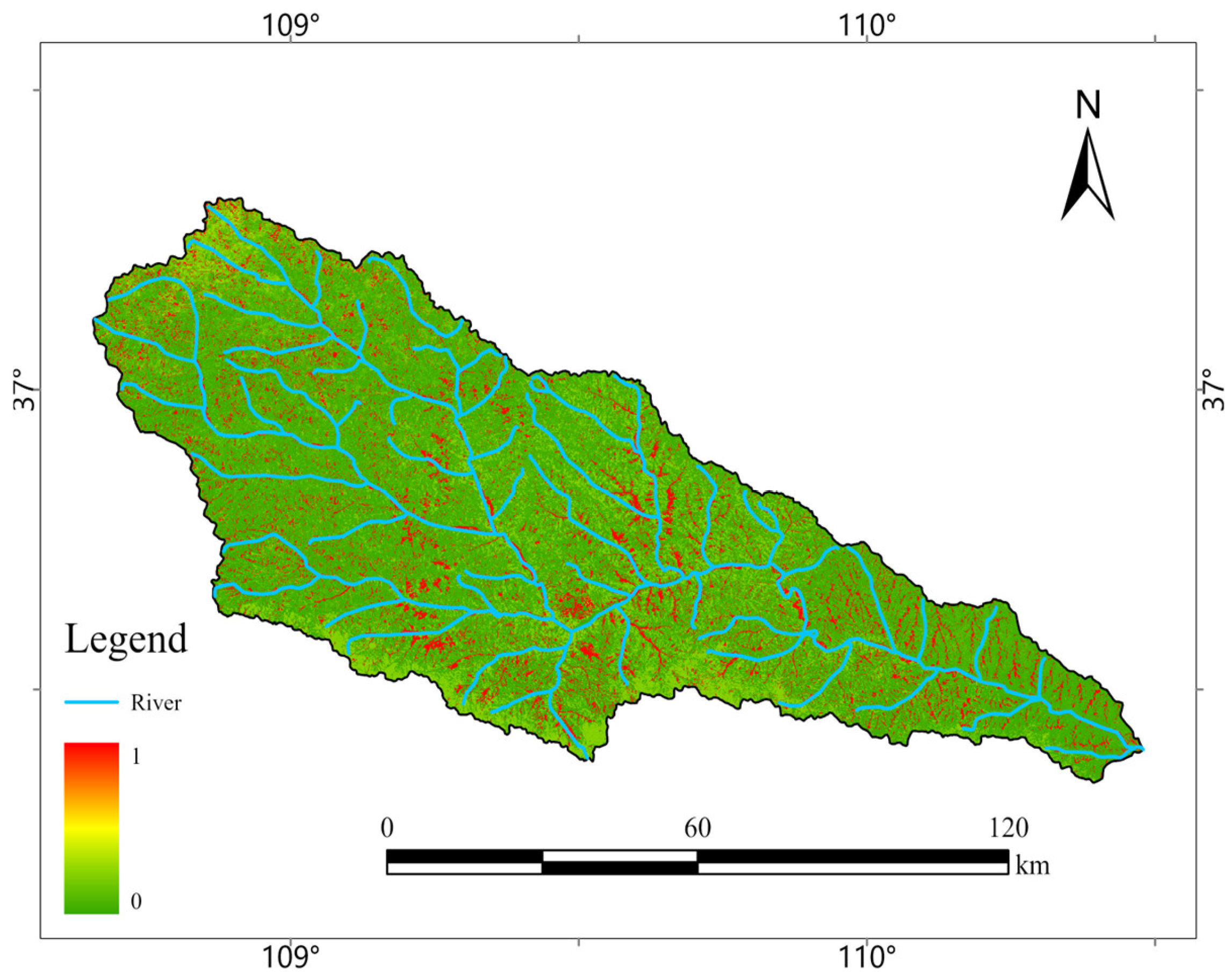
- Based on the average FVC of the 24 half-months, the B-factor was assessed by considering land use types and the proportion of rainfall erosivity factors during this period (Figure 3).
3.3. Image Processing
3.4. Calculation of the B-Factor
4. Results
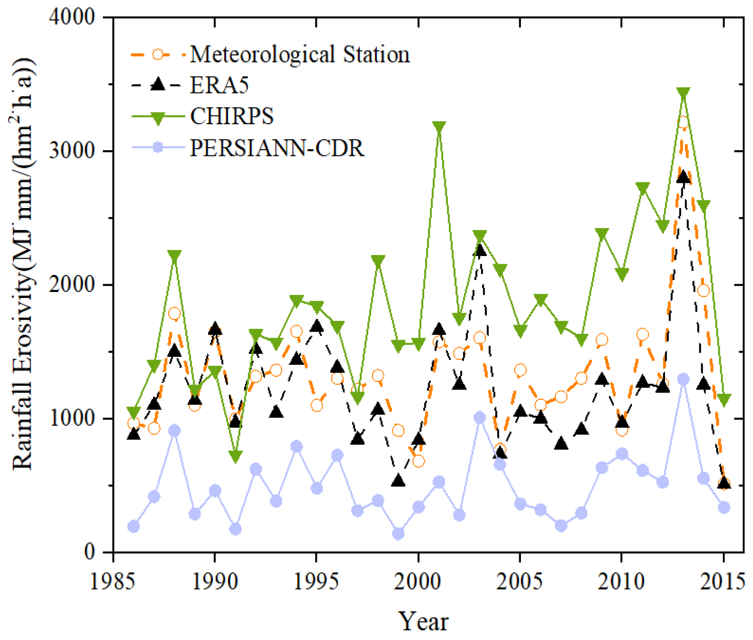
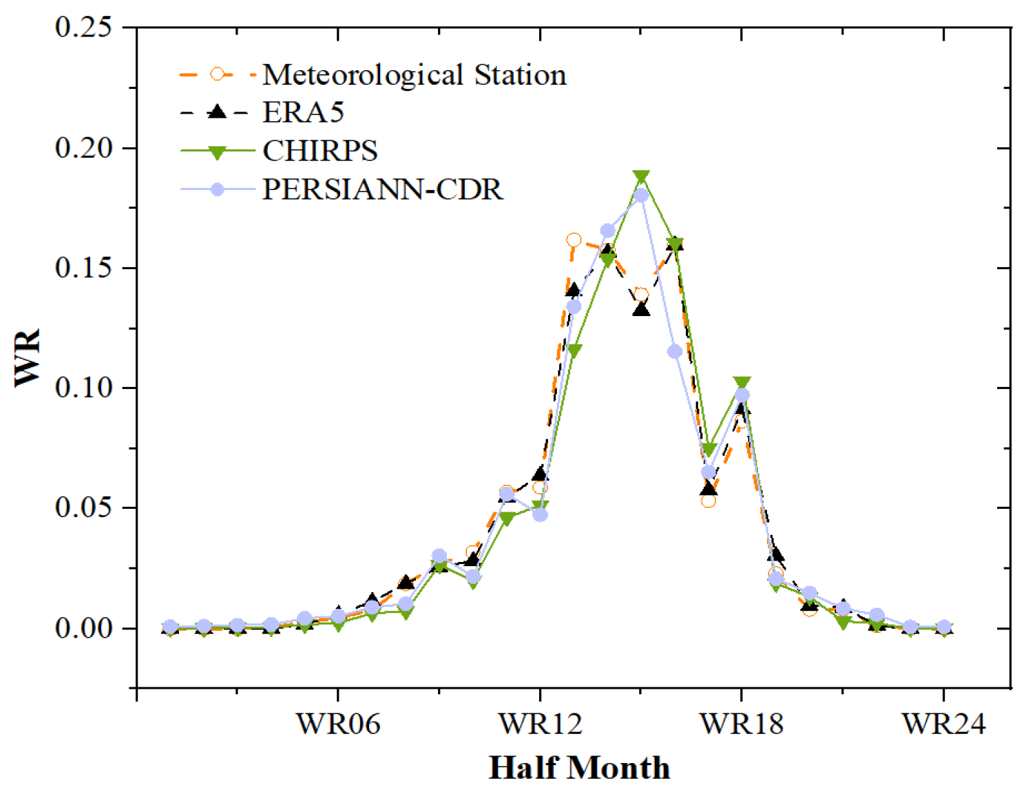
4.1. Applicability of Different Rainfall Datasets in the Yanhe River Basin
4.2. The NDVI Calculated by Patched Sentinel-2 Images
4.3. Assessment of Vegetation Cover and Biological Measures’ B-Factor
5. Discussion
5.1. Applicability of Different Rainfall Datasets in the Yanhe River Basin
5.2. The NDVI and B-Factor Calculated Using Patched Sentinel-2 Images
5.3. Assessment of Vegetation Cover and Biological Measures’ B-Factor
6. Conclusions
- (1)
- The ERA5 precipitation dataset exhibited strong agreement with meteorological station data across various metrics including average erosive rainfall, average erosive rainfall intensity, average rainfall erosivity, and WR over multiple years. It demonstrated better suitability for the Yanhe River Basin compared to the CHIRPS and PERSIANN-CDR datasets, making it a viable alternative for calculating rainfall erosivity in the absence of meteorological station data.
- (2)
- This study proposed a new and simple method, the trend migration method, for patching missing Sentinel-2 data based on the rate of change of the image in time. Sentinel-2 modified by the trend migration approach outperformed the HANTS method in terms of data authenticity. The restored high-resolution Sentinel-2 data fit nicely with the 10 m resolution land use data, enhancing the B-factor calculation accuracy from the regional to the spot level.
- (3)
- In the GEE environment, we developed a fully automated B-factor calculation procedure, and the B-factor was assessed and mapped efficiently based on rainfall erosivity, soil loss rate, vegetation covering, and land use types in the Yanhe River Basin. The computation procedure is broadly applicable and can be extended to various river basins as well as wider regional scales, which provides data and technical support for regional soil erosion monitoring.
Author Contributions
Funding
Data Availability Statement
Acknowledgments
Conflicts of Interest
References
- Leng, S.Y.; Feng, R.G.; Li, R. Key Research Issues of Soil Erosion and Conservation in China. J. Soil Water Conserv. 2004, 18, 1–6. [Google Scholar]
- Shi, P.J.; Liu, B.Y.; Zhang, K.L.; Jin, Z. Soil Erosion Process and Model Studies. Resour. Sci. 1999, 21, 9–18. [Google Scholar]
- Li, Z.; Zhu, B.; Li, P. Advancement in Study on Soil Erosion and Soil and Water Conservation. Acta Pedol. 2008, 45, 802–809. [Google Scholar]
- Cai, Q.; Liu, J. Evolution of Soil Erosion Models in China. Prog. Geogr. 2003, 22, 242–250. [Google Scholar]
- Fu, B.; Liu, Y.; Lü, Y.; He, C.; Zeng, Y.; Wu, B. Assessing the Soil Erosion Control Service of Ecosystems Change in the Loess Plateau of China. Ecol. Complex. 2011, 8, 284–293. [Google Scholar] [CrossRef]
- Lin, J.; Guan, Q.; Tian, J.; Wang, Q.; Tan, Z.; Li, Z.; Wang, N. Assessing Temporal Trends of Soil Erosion and Sediment Redistribution in the Hexi Corridor Region Using the Integrated RUSLE-TLSD Model. CATENA 2020, 195, 104756. [Google Scholar] [CrossRef]
- Liu, B.; Zhang, K.; Xie, Y. An Empirical Soil Loss Equation. In Proceedings of the 12th International Soil Conservation Organization Conference, Beijing, China, 26 May 2002; pp. 26–31. [Google Scholar]
- Shi, W.; Huang, M.; Barbour, S.L. Storm-Based CSLE That Incorporates the Estimated Runoff for Soil Loss Prediction on the Chinese Loess Plateau. Soil Tillage Res. 2018, 180, 137–147. [Google Scholar] [CrossRef]
- Ayalew, D.A.; Deumlich, D.; Šarapatka, B.; Doktor, D. Quantifying the Sensitivity of NDVI-Based C Factor Estimation and Potential Soil Erosion Prediction using Spaceborne Earth Observation Data. Remote Sens. 2020, 12, 1136. [Google Scholar] [CrossRef]
- Biddoccu, M.; Guzman, G.; Capello, G.; Thielke, T.; Strauss, P.; Winter, S.; Zaller, J.G.; Nicolai, A.; Cluzeau, D.; Popescu, D.; et al. Evaluation of soil erosion risk and identification of soil cover and management factor (C) for RUSLE in European vineyards with different soil management. Int. Soil Water Conserv. Res. 2020, 8, 337–353. [Google Scholar] [CrossRef]
- Pinson, A.O.; AuBuchon, J.S. A new method for calculating C factor when projecting future soil loss using the Revised Universal soil loss equation (RUSLE) in semi-arid environments. CATENA 2023, 226, 107067. [Google Scholar] [CrossRef]
- Yin, S.; Zhu, Z.; Wang, L.; Liu, B.; Xie, Y.; Wang, G.; Li, Y. Regional Soil Erosion Assessment Based on a Sample Survey and Geostatistics. Hydrol. Earth Syst. Sci. 2018, 22, 1695–1712. [Google Scholar] [CrossRef]
- Xu, Y.; Ding, Y.; Zhao, Z. Confidence Analysis of NCEP/NCAR 50-Year Global Reanalyzed Data in Climate Change Research in China. J. Appl. Meteorol. 2001, 12, 337–347. (In Chinese) [Google Scholar]
- Zhao, T.; Ai, L.; Feng, J.M. An Intercomparison between NCEP Reanalysis and Observed Data over China. Clim. Environ. Res. 2004, 9, 278–294. (In Chinese) [Google Scholar]
- Wang, Z.; Zhong, R.; Chen, J.; Huang, W. Evaluation of Drought Utility Assessment of TMPA Satellite-Remote-Sensing-Based Precipitation Product in Mainland China. CSAE 2017, 33, 163–170. (In Chinese) [Google Scholar]
- Cai, Y.; Jin, C.; Wang, A.; Guan, D.; Wu, J.; Yuan, F.; Xu, L. Comprehensive Precipitation Evaluation of TRMM 3B42 with Dense Rain Gauge Networks in a Mid-Latitude Basin, Northeast, China. Theor. Appl. Climatol. 2016, 126, 659–671. [Google Scholar] [CrossRef]
- Liu, H.; Zhang, M.; Lin, Z.; Xu, X. Spatial Heterogeneity of the Relationship between Vegetation Dynamics and Climate Change and Their Driving Forces at Multiple Time Scales in Southwest China. Agric. For. Meteorol. 2018, 256–257, 10–21. [Google Scholar] [CrossRef]
- Li, M.; Zhang, Y. Temporal and spatial variation characteristics and influencing factors of vegetation cover in the middle Yellow River Basin. J. Guizhou Norm. Univ. Nat. Sci. 2023, 41, 10–20. (In Chinese) [Google Scholar]
- Jiang, W.; Yuan, L.; Wang, W.; Cao, R.; Zhang, Y.; Shen, W. Spatio-Temporal Analysis of Vegetation Variation in the Yellow River Basin. Ecol. Indic. 2015, 51, 117–126. [Google Scholar] [CrossRef]
- Gorelick, N.; Hancher, M.; Dixon, M.; Ilyushchenko, S.; Thau, D.; Moore, R. Google Earth Engine: Planetary-Scale Geospatial Analysis for Everyone. Remote Sens. Environ. 2017, 202, 18–27. [Google Scholar] [CrossRef]
- Zhang, B. Remotely Sensed Big Data Era and Intelligent Information Extraction. Geomat. Inf. Sci. Wuhan Univ. 2018, 43, 1861–1871. (In Chinese) [Google Scholar]
- Wen, Z.; Jiao, F.; Jiao, J. Prediction and mapping of potential vegetation distribution in Yanhe River catchment in hilly area of Loess Plateau. Chin. J. Appl. Ecol. 2008, 19, 1897–1904. (In Chinese) [Google Scholar]
- Ashouri, H.; Hsu, K.; Sorooshian, S.; Braithwaite, D.; Knapp, K.; Cecil, L.; Nelson, B.; Prat, O.P. PERSIANN-CDR: Daily Precipitation Climate Data Record from Multisatellite Observations for Hydrological and Climate Studies. Bull. Amer. Meteor. Soc. 2015, 96, 69–83. [Google Scholar] [CrossRef]
- Roerink, G.J.; Menenti, M.; Verhoef, W. Reconstructing Cloudfree NDVI Composites Using Fourier Analysis of Time Series. Int. J. Remote Sens. 2000, 21, 1911–1917. [Google Scholar] [CrossRef]
- Zhou, J.; Jia, L.; Menenti, M. Reconstruction of Global MODIS NDVI Time Series: Performance of Harmonic ANalysis of Time Series (HANTS). Remote Sens. Environ. 2015, 163, 217–228. [Google Scholar] [CrossRef]
- Liu, B.Y.; Xie, Y.; Li, Z.Y.; Liang, Y.; Zhang, W.B.; Fu, S.H.; Yin, S.Q.; Wei, X.; Zhang, K.L.; Wang, Z.Q.; et al. The assessment of soil loss by water erosion in China. Int. Soil Water Conserv. Res. 2020, 8, 430–439. [Google Scholar] [CrossRef]
- Yang, X.; Zhu, Q.; Tulan, M.; McInnes-Clarke, S.; Sun, L.; Zhang, X.P. Near real-time monitoring of post-fire erosion after storm events: A case study in Warrumbungle National Park, Australia. Int. J. Wildland Fire 2018, 27, 413–422. [Google Scholar] [CrossRef]
- Guerschman, J.P.; Hill, M.J.; Renzullo, L.J.; Barrett, D.J.; Marks, A.S.; Botha, E.J. Estimating fractional cover of photosynthetic vegetation, non-photosynthetic vegetation and bare soil in the Australian tropical savanna region upscaling the EO-1 Hyperion and MODIS sensors. Remote Sens. Environ. 2009, 113, 928–945. [Google Scholar] [CrossRef]
- Huang, C. Study on the Spatiotemporal Variation of Soil Erosion in the Loess Plateau over the Past 40 Years and Its Controlling Factors. Ph.D. Thesis, Northwest University, Kirkland, WA, USA, 2021. (In Chinese). [Google Scholar]
- Yang, S.; Quan, Q.; Xu, J.; Zhang, F.; Liu, T. Water Conservation Function in the Process of Land Use Change in Yanhe River Basin. Soil Water Conserv. Chin. 2022, 33–36. (In Chinese) [Google Scholar] [CrossRef]


| Land Use Types | Area (km2) | Proportions |
|---|---|---|
| Forestland | 1151.02 | 14.98% |
| Shrubland | 0.0166 | 0.00% |
| Grassland | 5358.8 | 69.76% |
| Cultivated land | 528.086 | 6.87% |
| Building land | 101.481 | 1.32% |
| Unused land | 535.108 | 6.97% |
| Water body | 6.9805 | 0.09% |
| Wetland | 0.0569 | 0.00% |
| Datasets | Name | Period (Day) | Resolution (m) | Period |
|---|---|---|---|---|
| MODIS | MOD09GA | 1 | 500 | 2000–2023 |
| Landsat 7 | LE07/C02/T1_L2 | 8 | 30 | 1999–2023 |
| Landsat 8 | LC08/C02/T1_L2 | 8 | 30 | 2013–2023 |
| Sentinel 2 | S2_SR HARMONIZED | 5 | 10 | 2017–2023 |
| Half-Month | MOD09GA | Sentinel-2 | Landsat 8 | Landsat 7 | ||||
|---|---|---|---|---|---|---|---|---|
| Number of Available Images | Missing Rate | Number of Available Images | Missing Rate | Number of Available Images | Missing Rate | Number of Available Images | Missing Rate | |
| 1 | 45 | 0% | 27 | 0% | 6 | 10% | 6 | 55% |
| 2 | 48 | 0% | 35 | 0% | 5 | 0% | 8 | 6% |
| 3 | 45 | 0% | 31 | 0% | 5 | 41% | 9 | 3% |
| 4 | 40 | 0% | 18 | 0% | 6 | 0% | 3 | 46% |
| 5 | 45 | 0% | 21 | 0% | 7 | 9% | 9 | 6% |
| 6 | 48 | 0% | 32 | 0% | 8 | 0% | 10 | 17% |
| 7 | 45 | 0% | 14 | 56% | 3 | 1% | 2 | 92% |
| 8 | 45 | 0% | 33 | 0% | 8 | 0% | 9 | 11% |
| 9 | 45 | 0% | 35 | 0% | 8 | 0% | 9 | 10% |
| 10 | 48 | 0% | 43 | 0% | 6 | 0% | 8 | 2% |
| 11 | 45 | 0% | 34 | 0% | 8 | 45% | 3 | 40% |
| 12 | 45 | 0% | 21 | 0% | 2 | 81% | 1 | 55% |
| 13 | 45 | 0% | 33 | 0% | 6 | 16% | 9 | 0% |
| 14 | 48 | 0% | 30 | 0% | 2 | 30% | 2 | 91% |
| 15 | 45 | 0% | 35 | 0% | 5 | 6% | 5 | 35% |
| 16 | 48 | 0% | 33 | 0% | 6 | 0% | 1 | 90% |
| 17 | 45 | 0% | 38 | 0% | 6 | 63% | 9 | 2% |
| 18 | 45 | 0% | 31 | 0% | 6 | 3% | 7 | 9% |
| 19 | 45 | 0% | 9 | 56% | 0 | 100% | 2 | 48% |
| 20 | 48 | 0% | 35 | 0% | 2 | 1% | 8 | 25% |
| 21 | 45 | 0% | 51 | 0% | 7 | 62% | 9 | 2% |
| 22 | 45 | 0% | 27 | 0% | 5 | 1% | 9 | 1% |
| 23 | 45 | 0% | 45 | 0% | 6 | 0% | 9 | 8% |
| 24 | 48 | 0% | 38 | 0% | 10 | 0% | 8 | 7% |
| Total | 1096 | 0% | 749 | 5% | 133 | 20% | 155 | 27% |
| Land Use (Class I) | Land Use (Class II) | B-Factor Value | Description |
|---|---|---|---|
| Cultivated land | Paddy field | 1 | Soil and water conservation benefits reflected by tillage measure factor |
| Irrigated land | 1 | Soil and water conservation benefits reflected by tillage measure factor | |
| Dry land | 1 | Soil and water conservation benefits reflected by tillage measure factor | |
| Residential, industrial, and mining lands | Urban residential lands | 0.01 | Equivalent to 80% of vegetation cover |
| Rural residential lands | 0.025 | Equivalent to 60% of vegetation cover | |
| Independent industrial and mining lands | 1 | Equivalent to no vegetation cover | |
| Commercial service and public lands | 0.01 | Equivalent to 80% of vegetation cover | |
| Special land use | 0.1 | ||
| Land for transportation | 0.01 | Equivalent to 80% of vegetation cover | |
| Land for water area and water conservancy facilities | 0 | Forced to 0, so that the amount of erosion is equal to 0 | |
| Other land | Saline alkali soil | 0 | - |
| Sandy land | 0 | - | |
| Swamp land | 0 | - | |
| Bare rock | 0 | - | |
| Bare soil | 1 | - | |
| Glaciers and permanent snow cover | 0 | - |
| Rainfall Parameters | Meteorological Station | ERA5 | CHIRPS | PERSIANN-CDR |
|---|---|---|---|---|
| Annual average rainfall (mm) | 467 | 570 | 481 | 455 |
| Average annual erosive rainfall (mm) | 283 | 288 | 332 | 128 |
| Multi-year average erosive rainfall days (mm day−1) | 22 | 22 | 28 | 20 |
| Multi-year average number of days of erosive rainfall (day) | 12 | 13 | 12 | 6 |
| Multi-year average rainfall erosivity (MJ·mm hm−2 h−1 yr−1) | 1327 | 1222 | 1876 | 502 |
Disclaimer/Publisher’s Note: The statements, opinions and data contained in all publications are solely those of the individual author(s) and contributor(s) and not of MDPI and/or the editor(s). MDPI and/or the editor(s) disclaim responsibility for any injury to people or property resulting from any ideas, methods, instructions or products referred to in the content. |
© 2024 by the authors. Licensee MDPI, Basel, Switzerland. This article is an open access article distributed under the terms and conditions of the Creative Commons Attribution (CC BY) license (https://creativecommons.org/licenses/by/4.0/).
Share and Cite
Wu, Y.; Shi, H.; Yang, X. Estimating the CSLE Biological Conservation Measures’ B-Factor Using Google Earth’s Engine. Remote Sens. 2024, 16, 847. https://doi.org/10.3390/rs16050847
Wu Y, Shi H, Yang X. Estimating the CSLE Biological Conservation Measures’ B-Factor Using Google Earth’s Engine. Remote Sensing. 2024; 16(5):847. https://doi.org/10.3390/rs16050847
Chicago/Turabian StyleWu, Youfu, Haijing Shi, and Xihua Yang. 2024. "Estimating the CSLE Biological Conservation Measures’ B-Factor Using Google Earth’s Engine" Remote Sensing 16, no. 5: 847. https://doi.org/10.3390/rs16050847
APA StyleWu, Y., Shi, H., & Yang, X. (2024). Estimating the CSLE Biological Conservation Measures’ B-Factor Using Google Earth’s Engine. Remote Sensing, 16(5), 847. https://doi.org/10.3390/rs16050847