Review

Meta-Analysis Assessing Potential of Drone Remote Sensing in Estimating Plant Traits Related to Nitrogen Use Efficiency

1
Precision Agriculture Laboratory, School of Life Sciences, Technical University of Munich, 85354 Freising, Germany
2
Inner Mongolia Key Laboratory of Soil Quality and Nutrient Resources, Key Laboratory of Agricultural Ecological Security and Green Development at Universities of Inner Mongolia Autonomous, Hohhot 010018, China
3
Electronics and Precision Agriculture Lab (EPAL), Department of Agricultural Engineering, Sokoine University of Agriculture, Morogoro 30007, Tanzania
4
World Agricultural Systems Center, Technical University of Munich, 85354 Freising, Germany
*
Author to whom correspondence should be addressed.
Remote Sens. 2024, 16(5), 838; https://doi.org/10.3390/rs16050838
Submission received: 16 December 2023 / Revised: 5 February 2024 / Accepted: 22 February 2024 / Published: 28 February 2024
(This article belongs to the Section Remote Sensing in Agriculture and Vegetation)

Abstract

:
Unmanned Aerial Systems (UASs) are increasingly vital in precision agriculture, offering detailed, real-time insights into plant health across multiple spectral domains. However, this technology’s precision in estimating plant traits associated with Nitrogen Use Efficiency (NUE), and the factors affecting this precision, are not well-documented. This review examines the capabilities of UASs in assessing NUE in crops. Our analysis specifically highlights how different growth stages critically influence NUE and biomass assessments in crops and reveals a significant impact of specific signal processing techniques and sensor types on the accuracy of remote sensing data. Optimized flight parameters and precise sensor calibration are underscored as key for ensuring the reliability and validity of collected data. Additionally, the review delves into how different canopy structures, like planophile and erect leaf orientations, uniquely influence spectral data interpretation. The study also recognizes the untapped potential of image texture features in UAV-based remote sensing for detailed analysis of canopy micro-architecture. Overall, this research not only underscores the transformative impact of UAS technology on agricultural productivity and sustainability but also demonstrates its potential in providing more accurate and comprehensive insights for effective crop health and nutrient management strategies.

1. Introduction

Nitrogen plays a crucial role as the primary limiting nutrient for essential processes in plants, including photosynthesis, regulation of phytohormones such as auxins and cytokinins, and proteomic changes throughout their lifecycle [1]. However, the excessive and inefficient use of nitrogen fertilizers not only increases crop production costs but also leads to environmental issues such as soil degradation, water pollution, and biodiversity loss [2]. To address these challenges, it is essential to assess the efficiency of nitrogen utilization in crop production and evaluate its potential environmental impacts. Nitrogen Use Efficiency (NUE) is a measure of how effectively a plant utilizes available nitrogen for growth. A variety of indicators of NUE are widely used for this purpose. NUE is critical in understanding nitrogen cycles and guiding nitrogen management practices. By accurately measuring NUE, we can optimize nitrogen application, minimize wastage and leaching to soil, and improve crop yield without compromising environmental sustainability. To date, several methods have been employed for plant NUE assessment, including the system nitrogen balances methods [3], calculated by comparing the difference between nitrogen inputs and nitrogen outputs [4]; soil-based methods which focus on the rate of soil nitrogen mineralization, nitrification, and denitrification [5]; plant-based methods which involve the nitrogen content collected and analyzed from plant tissues [6]; and isotope-labeled method which could track the fate and movement of nitrogen in the soil-plant system [7]. In addition, with the development of remote sensing technologies, research is increasingly using images taken by satellites and drones to monitor arable crops [8,9] and estimate NUE over large area cropping systems [10] for a more comprehensive understanding of NUE in a spatially explicit manner.
Drones, distinct from other remote sensing technologies, provide unparalleled flexibility and accessibility. They can transmit data in real-time, allowing for immediate analysis and decision-making [11]. Combining different kinds of sensors with high spatial resolution imagers (i.e., Multispectral (MS), Hyperspectral (HSI), thermal, Light Detection and Ranging (LiDAR)), it can be used for different types of monitoring tasks such as drought stress [12], yield prediction [13], weed detection [14], nitrogen status [15], growth vigor [16]. So far, there have been articles on drone remote sensing-based assessment of NUE. For instance, Yang et al. [17] predicted the NUE variations among the winter wheat genotypes, where it was discovered that drone-carrying MS cameras can effectively predict time-series of NUE throughout the growing season. This study has proved valuable in selecting elite genotypes and monitoring crop performance under various nitrogen treatments. Liang et al. [18] used UAV-based MS imagery to identify high NUE varieties of rice through the entire growth duration. Their investigation indicated that UASs have immense potential to determine NUE phenotypes.
The findings from these studies highlight the significant capability of drones in NUE assessment. While the progression of UASs enhances the scope and precision of NUE assessments across various crops and agricultural practices, it also presents several challenges. Key among these are the inconsistencies arising from variations in growth stage, signal processing technology, and sensor type [18]. Additionally, it is important to emphasize that different methods of calculating NUE might result in significant variations in NUE values, even when applied within the same experimental field and cropping system [19]. Therefore, it is critical to select and standardize the most appropriate UAV remote sensing metrics for assessing NUE to ensure accuracy and consistency. This review aims (i) to examine the moderators which affect remote sensing of crop nitrogen status; (ii) to quantify the effects of various influencing moderators on crop NUE; (iii) evaluate the potential of UASs for remote assessment of NUE quantitatively; and (iv) provide recommendations for optimizing UAS technology for NUE assessment in agricultural practices.

2. Materials and Methods

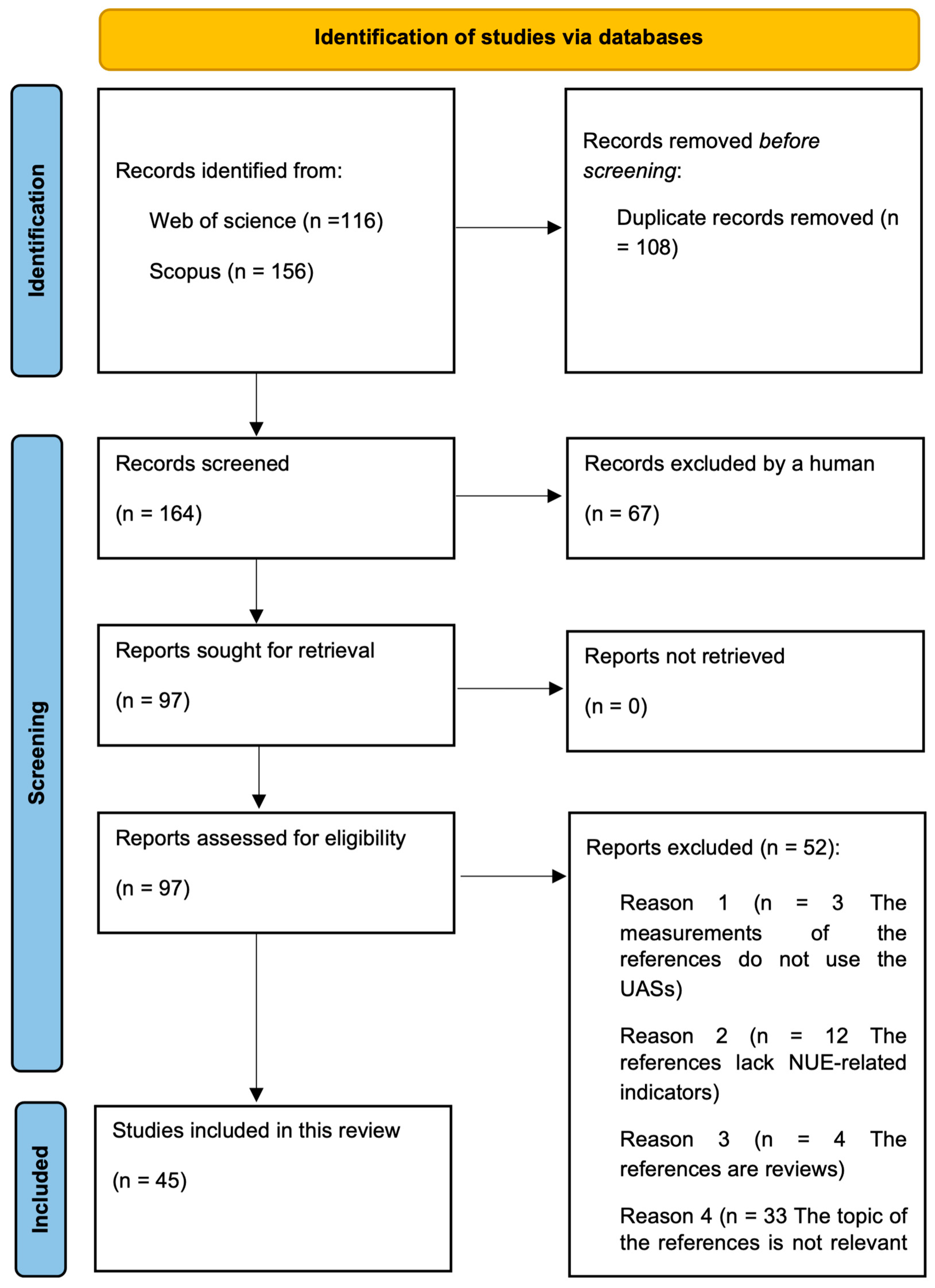
2.1. Literature Search

Using the PRISMA protocol, we conducted a systematic review and meta-analysis of studies that use UAVs to estimate NUE in agricultural systems. Figure 1 presents a flow diagram of the study selection process. In the identification step, relevant literature was retrieved from Scopus and Web of Science using search terms comprising keywords related to UAVs and nitrogen use efficiency (shown in Appendix S2). The search was limited to English-language research articles published from 1 January 1995 to 20 January 2024. The studies classified as review papers, book chapters, reports, Ph.D. theses or errata were not considered.
A total of 164 articles were obtained from the Scopus and Web of Sciences searches. To be included in the review, a study was required to fulfill the following three criteria: (i) the study uses UAS type; (ii) it focuses on vegetation NUE; (iii) it uses at least one of the NUE indicators. A total of 35 studies were included in the quantitative analysis, as they met the criteria and provided extractable data for all features. For each article, we extracted metadata, including information related to the characteristics of the location, vegetation, measurement period, sensor type, signal processing technique, vegetation index, R 2 , and NUE indicators manually (Appendix S1).

2.2. Data Extraction

Typically, the NUE is gauged in an indirect manner by measuring a suite of N-related crop and/soil traits. The plant traits pertinent to the assessment of NUE typically encompass plant nitrogen content and uptake, grain protein content, biomass, and yield. These traits are intrinsically linked to the calculation and assessment of NUE. Plant N-related traits such as nitrogen content, leaf chlorophyll content, and protein content offer an in-depth insight into the plant’s nitrogen dynamics. Similarly, attributes like biomass, yield, and plant height, while serving as indicators, also elucidate the associations between plant vitality and its nitrogen consumption. Moreover, the (Leaf Area Index) LAI and the Thousand Grain Weight (TGW) reveal the plant’s photosynthetic efficiency and grain morphological characteristics, which are both closely influenced by N-related traits and trait interactions [20,21]. Figure 2 summarizes the plant traits we extracted from the literatures and used in this review for the NUE evaluation included. For a comprehensive and robust meta-analysis, we honed our focus on six core trait categories directly related to NUE: nitrogen content (covering both Plant Nitrogen Content (PNC), Plant Nitrogen Weight (PNW), and Plant Nitrogen Accumulation (PNA)), biomass, direct NUE measurements, LAI, Plant Height, and Grain Yield. Ensuring the validity of our research, we included only those studies that transparently reported both the coefficient of determination ( R 2 ) and the associated sample size for each trait in the quantitative analysis section. Through our analysis, we pinpointed five pivotal variables (i.e., Sensor Types, Signal Processing Techniques, Model Evaluation Procedures, Growth Stages, and Crop Types) that influence the accuracy of plant trait estimation:
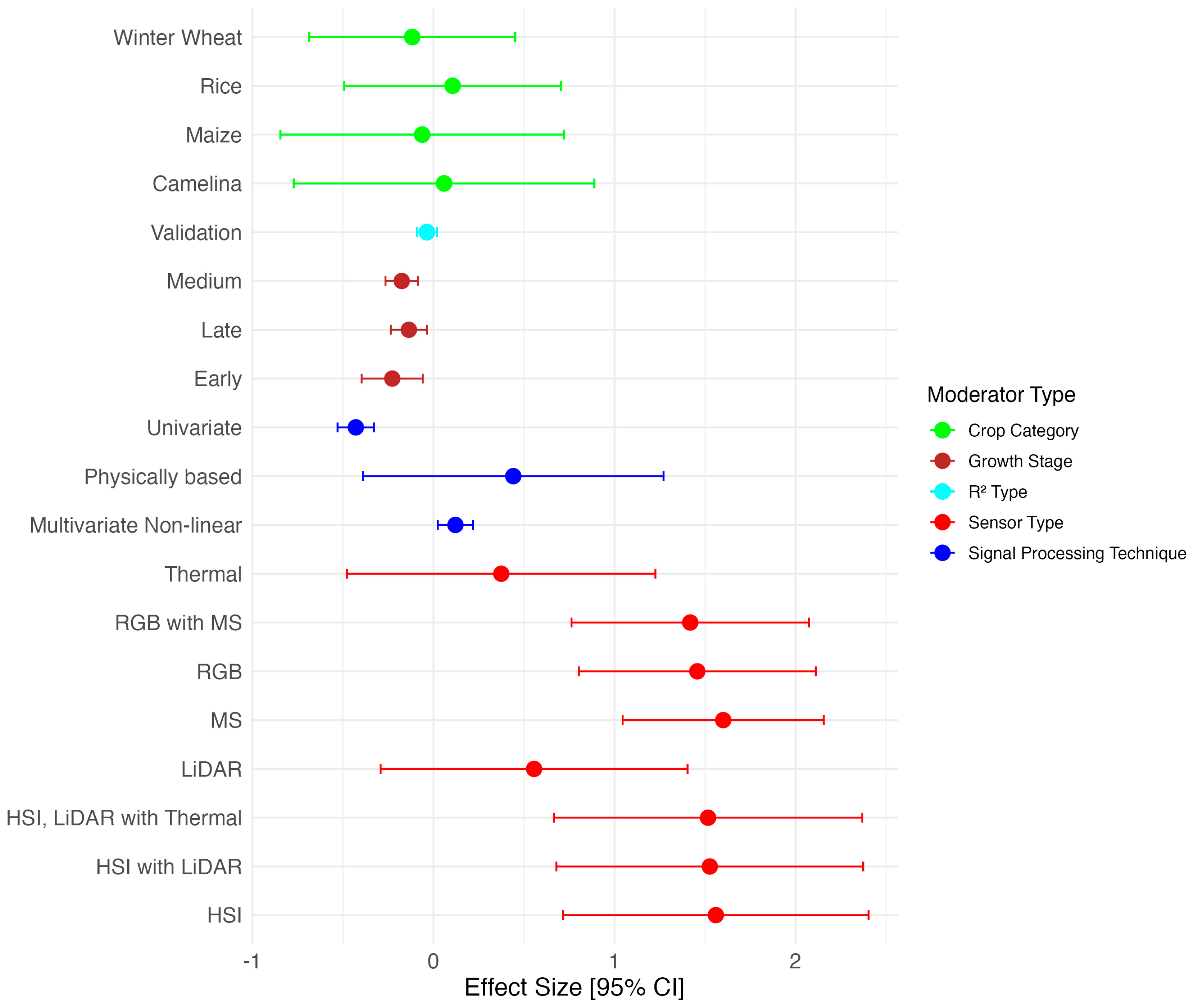
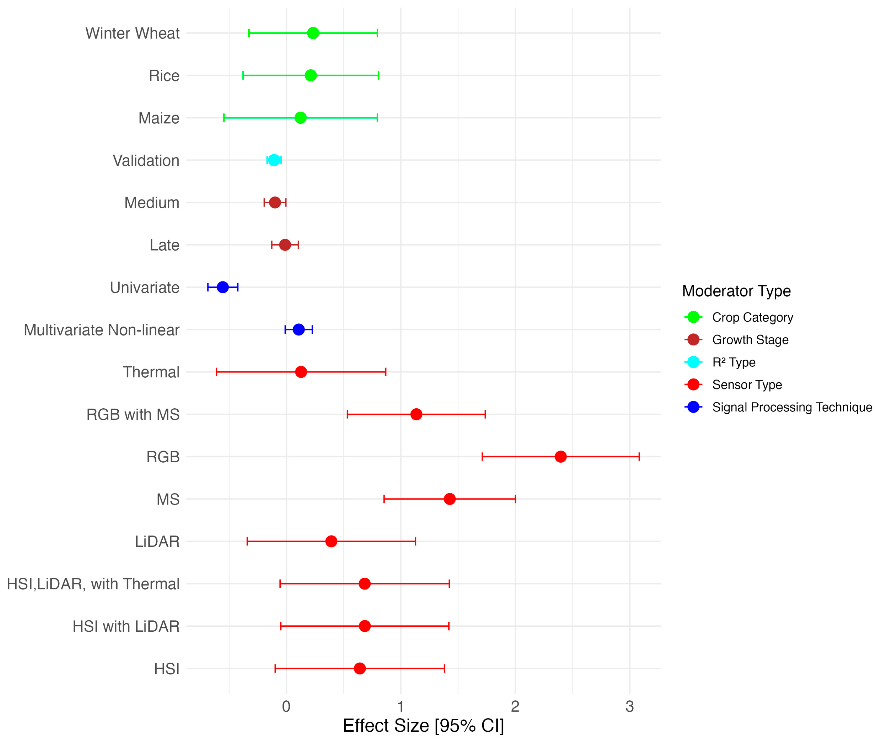
  • Sensor Types: We identified four sensor types that could potentially influence the accuracy of trait estimation: RGB, MS, HSI, and a combination of RGB and MS sensors.
  • Signal Processing Techniques: To estimate vegetation characteristics, we employed a range of signal processing techniques as outlined by [22]. These include Multivariate Linear Methods (e.g., Partial Least Squares Regression, Stepwise Multiple Linear Regression, and Multiple Linear Regression), Multivariate Non-Linear Methods (e.g., Random Forest and Support Vector Machine), Physically Based Approaches (utilizing specific formulas), and Univariate Methods (involving Vegetation Indices and either Linear or Non-Linear Regressions).
  • Model Evaluation Procedures: In the existing literature, two predominant strategies for model evaluation are calibration and validation. Calibration R 2 serves as a measure of the model’s accuracy when derived from a training data set. In contrast, validation R 2 gauges the model’s capacity for estimating trait values in an independent test data set, thereby providing insights into the model’s generalizability and stability.
  • Growth Stages: To standardize the data monitoring period across all studies, we converted the reported growth stages to the BBCH scale [23], a globally recognized scale for phenological staging in plants. We categorized the growth stages as follows: early stage (BBCH 0–30), mid-stage (BBCH 31–60), and late stage (BBCH 61–90). Additionally, we considered the entire growth period (BBCH 0–90) as a separate category. These categorizations were employed to assess the impact of different growth stages on the accuracy of plant trait prediction.
  • Crop Types: The articles analyzed for prediction accuracy primarily focused on the following crops: winter wheat, maize, barley, winter oilseed, and rice. These crops were individually categorized to evaluate the differential impact of crop type on the accuracy of plant trait estimation.

2.3. Data Analysis

In evaluating plant traits estimation accuracy within this meta-analysis, R 2 is chosen as our primary metric due to its wide acceptance and ease of interpretation. While both R 2 and Normalized Root Mean Squared Error (nRMSE) are valuable for quantifying accuracy, the latter is less commonly reported in the literature, limiting our ability to perform a comprehensive analysis. It is acknowledged that variances in reported accuracies exist both between and within individual studies. Between-study discrepancies often arise from contextual differences such as geographical location and types of drones used in data collection. Additionally, within the same study, variations in traits estimation accuracy can also be observed, attributable to the application of diverse signal processing techniques [22]. To quantitatively estimate these two sources of variance and identify the moderating variables that could influence the prediction accuracy, we utilize a three-level meta-analytic model, in line with established methodologies. This approach allows for a nuanced understanding of the factors contributing to accuracy disparities both within and across studies [24].

2.3.1. Data Transformation and Standardization

Plant traits estimation accuracy was typically expressed in terms of the R 2 . Initially, the data set is imported from a CSV file (Appendix S1) and cleaned to ensure robustness in the subsequent steps. This involves eliminating entries with missing R 2 values. Because meta-analytical three-level models assume normally distributed data [22] to enable a standardized comparison of accuracy across various studies. The R 2 values in their original form may not adhere to this assumption, especially in cases where the distribution of R 2 values is skewed or bounded. This non-normality can lead to analytical complications and potentially biased results in the meta-analysis. To address this issue and standardize the comparison of accuracy across different studies, we employed a mathematical transformation known as Fisher’s Z transformation. This transformation converts the R 2 values into a metric that approximates a normal distribution, thereby making it more suitable for our three-level meta-analytic model. This transformation is performed using the Equation (1):
Z = 1 2 ln ( 1 + r 1 r )
In this equation, Z represents the transformed value, and r is the square root of R 2 , also known as the correlation coefficient. This transformation is symmetric around zero, meaning that values of r close to 1 (high positive correlation) and −1 (high negative correlation) are transformed to positive and negative extremes, respectively, while an r value of 0 (no correlation) is transformed to 0 in the Z scale. The transformed values are less bounded compared to R 2 values, allowing for a more accurate estimation of effects and variances across studies.

2.3.2. Model Formulation: Three-Level Random Effects Model

Upon standardizing the data, the first step in our modeling exercise involves establishing a baseline model, commonly referred to as the “null” model. It does not yet include any predictors or moderator variables, allowing us to establish a benchmark for comparing other models that will include additional variables. This foundational model captures the overall effect size and provides initial estimates of between- and within-study variances. Mathematically, the null model is formulated as:
Z i j k = γ 00 + ν 0 k + μ j k + e i j k
here, Z i j k represents the observed Fisher’s Z value for the ith samples in the jth study from the kth data set. It is the outcome of the Fisher’s Z transformation applied to the R 2 values, as described previously. γ 00 (Grand Mean) is the intercept in this model, representing the overall mean effect size across all studies when all other effects are zero. This is the expected value of the transformed effect size when the random effects due to study are not present. ν 0 κ (Random Effect of Data Set—Level 3) represents the random effect due to the kth data set. It accounts for the variation in effect sizes between different data sets that cannot be explained by the overall mean alone. This term allows each data set to have its own unique effect size, which is assumed to be normally distributed around the γ 00 . μ j k (Random Effect of Study within Data Set—Level 2) represents the random effect due to the jth study within the kth data set. It captures the variability in effect sizes that occurs between studies within the same data set. This allows for the acknowledgment that different studies may have unique characteristics influencing their outcomes. e i j k (Random Effect of Sample within Study—Level 1) represents the random effect due to the ith sample within the jth study and kth data set. It is essentially the error term that represents the unexplained variance after considering the effects of the data set and the study. This includes measurement errors, individual sample variability, and other idiosyncratic factors affecting the Fisher’s Z value.

2.3.3. Incorporating Moderator Variables (Fixed Effect)

To delve deeper into the nuances of traits estimation accuracy, we expand this null model by incorporating moderating variables such as Sensor Type, Crop Type, Model Evaluation Procedures, Signal Processing Technique, and Growth Stage. These variables are introduced with the presumption that they systematically influence the traits estimation accuracy, thereby allowing us to explore the intricacies of the data more comprehensively.
Mathematically, the extended model can be expressed as follows, where Χ represents the matrix of moderator variables, and β represents the vector of coefficients associated with these moderators (Equation (3)):
Z i j k = γ 00 + Χ i j k β + ν 0 k + μ j k + e i j k
This equation now includes the term Χ i j k β , which captures the fixed effects of the moderator variables on the transformed effect size.

2.3.4. Assessing Variability and Intra-Class Correlation

Following the introduction of moderators, we measure the proportion of variance in the dependent variable that is attributable to the grouping structure in the data using the Intra-class Correlation Coefficient ( I C C ). The I C C is calculated using the Equation (4):
I C C = σ μ 2 σ μ 2 + σ ν 2
where σ μ 2 represents the estimated variance at the study level (Level 2). σ ν 2 represents the estimated variance at the data set level (Level 3). The I C C value ranges from 0 to 1. A high I C C suggests that the conditions or measurements within individual studies are significant contributors to the variability in traits estimation accuracy. Conversely, a low I C C would indicate that the variability (i.e., differences in geographical location, data collection protocols, etc.) between data sets is more pronounced.

2.3.5. Evaluating the Explained Variance

Finally, we assess the performance of the model by calculating the amount of variance explained by the moderating variables at both the study (Level 2) and data set (Level 3) levels. These are our overall levels in this analysis, and they help provide a comprehensive understanding of the data’s structure. This is performed using the following equations:
R 2 2 = 1 σ μ ( 1 ) 2 σ μ ( 0 ) 2
R 3 2 = 1 σ ν ( 1 ) 2 σ ν ( 0 ) 2
where R 2 2 and R 3 2 represent the proportion of the variance at the study level (Level 2) and data set level (Level 3), respectively. These metrics serve as robust indicators of the model’s explanatory power, providing valuable insights into the influence of moderating variables on traits estimation accuracy. A larger R 2 value indicates that a substantial portion of the variance is accounted for by the moderators, demonstrating their importance in the model. σ μ ( 1 ) 2 and σ ν ( 1 ) 2 represent the estimated variances at Levels 2 and 3, respectively, with moderator variables included. σ μ ( 0 ) 2 and σ ν ( 0 ) 2 represent the estimated variances at Levels 2 and 3, respectively, in the null model, without moderator variables.
By adopting this thorough methodological approach, we aim to offer a nuanced, robust, and comprehensive analysis, enhancing our understanding of traits estimation accuracy across a diverse array of conditions and studies.
The ‘lme4’ package (1.1.34), ‘nlme’ package (3.1.162), and ‘dplyr’ package (1.1.34) were used for data analysis, ‘ggplot2’ package (3.4.3) was used for data visualization in R (version 4.3.0).

3. Results

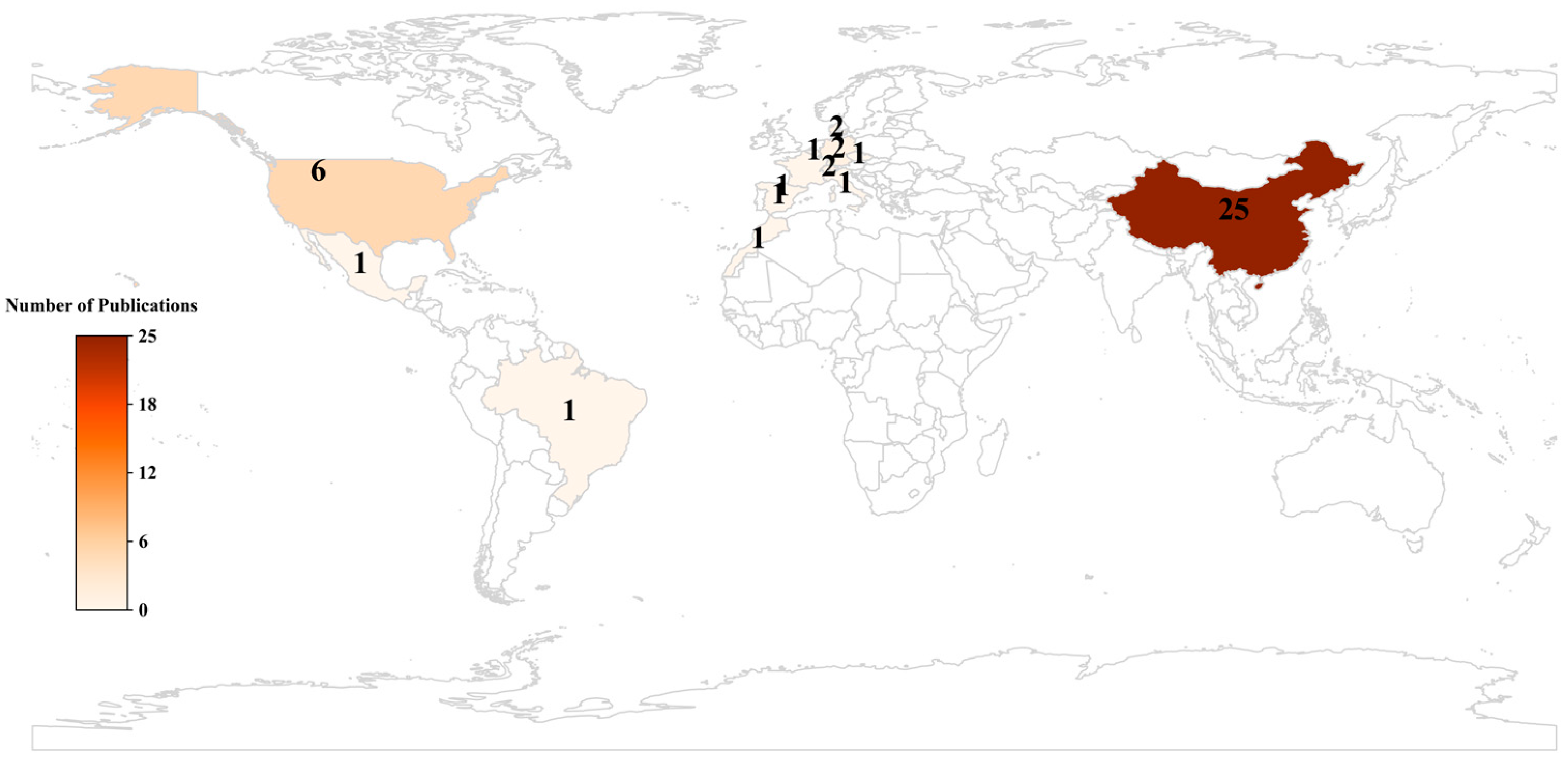
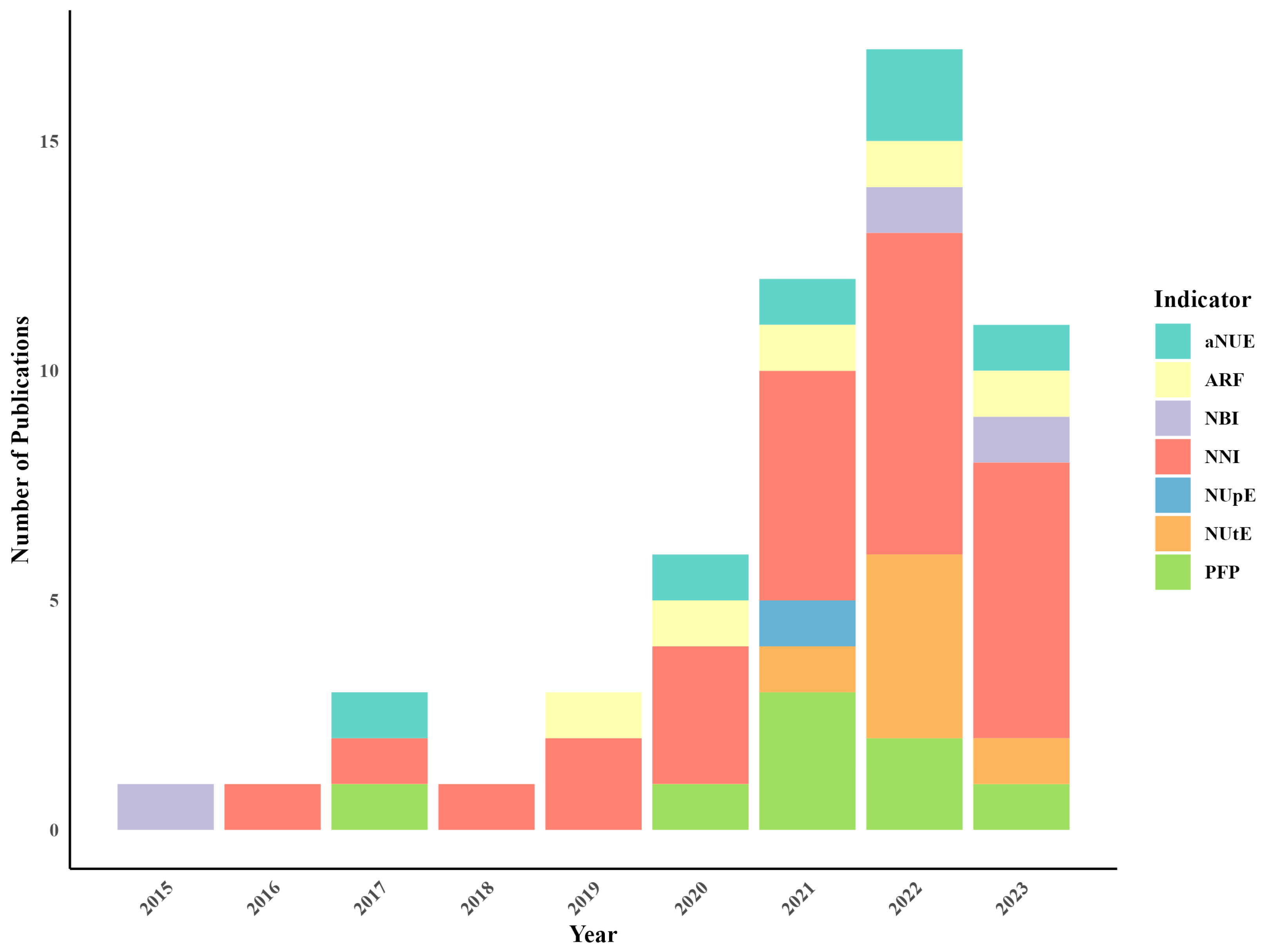
3.1. Geographical Distribution and Research Trends

Figure 3 depicts the geographical spread of the 45 studies encompassed in this review, spanning 13 different countries. In Asia, China emerges as a leading research hub with 25 studies, while in North America, the USA accounts for 6 studies. European research contributions were diverse. Germany, Denmark, and Switzerland presented two studies each, whereas Spain, France, Czechia, Italy, and Belgium had one study apiece. South America and Africa were represented by Brazil and Morocco, respectively, each contributing one study. From a climatic perspective, most studies focused on temperate regions, especially in Europe and the USA. However, the Brazilian study offered insights into tropical conditions, and arid perspectives were gleaned from studies in regions like Mexico and Morocco.
Climatic variations distinctly affect nitrogen absorption, transformation, and leaching [25]. For instance, rainwater can dissolve nitrogen in the soil and move it to deeper soil layers or into rivers, lakes, and groundwater. This leaching results in a significant loss of available nitrogen from the topsoil, affecting plant growth [26]. In arid regions, drought conditions might lead to nitrogen accumulation as they can inhibit plant growth, thus reducing nitrogen uptake [27]. It is evident that diverse climatic conditions necessitate distinct management strategies and technological applications.

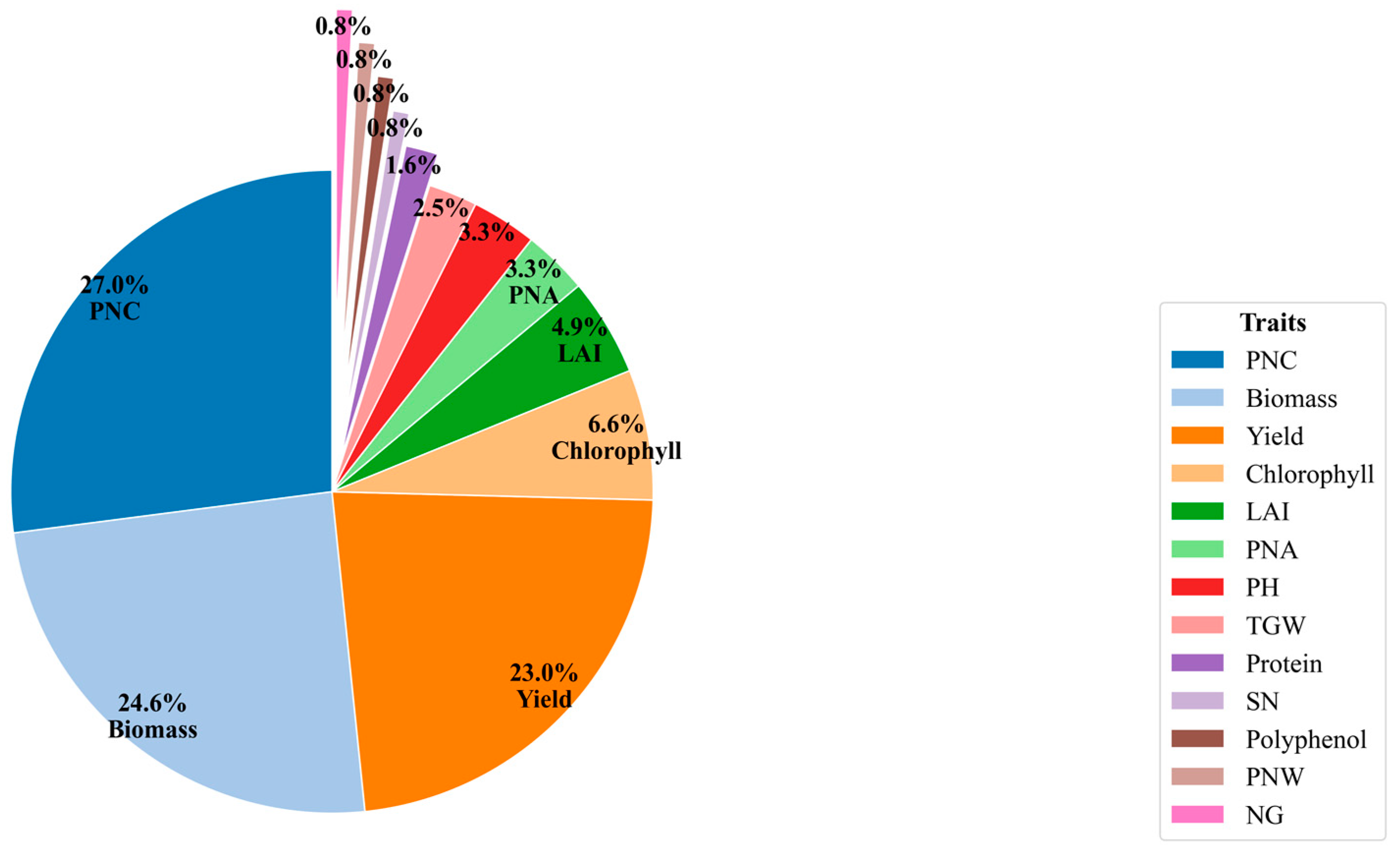
3.2. Comparing Indicators for Assessing NUE

Figure 4 presents the trend in the annual number of articles from 1995 to 2023, showcasing the various indicators used for assessing NUE. One of the first article, published in 2015 reported the use of the Nitrogen Balance Index (NBI) to precisely assess the nitrogen concentrations of paddy rice at a canopy level [28]. Subsequently, there has been a marked upswing in publications centered around utility of UAV remote sensing for NUE, which indicated the growing importance of assessing NUE for sustainable agriculture.
After rigorous screening, seven different indicators were extracted from the 45 references cited in this article. The Nitrogen Nutrition Index (NNI) was prominently featured [29], being referenced 26 times, showcasing a steady uptrend over time. Followed by the Partial Factor Productivity (PFP), which was mentioned in eight publications [30]. The agronomic Nitrogen Use Efficiency (aNUE) [31] and Nitrogen Utilization Efficiency (NutE) [18] were equally represented, each being mentioned in six studies. Among the indicators, the Nitrogen uptake Efficiency (NUpE) [32] was the least cited, appearing in 1 publication.
While NNI does not directly measure NUE, it assesses the nitrogen status in plants, providing insights into their nitrogen dynamics. NNI is calculated as the ratio of the actual N concentration to the critical N concentration, that is, the nitrogen concentration required for plants to achieve maximum growth rate (Equation (7)). While it provides insights into crop nitrogen dynamics, it differs from traditional metrics directly quantifying NUE [33]. Similarly, the chlorophyll-to-polyphenol ratio, known as the NBI (Equation (8)) [28], does not directly appraise NUE. Essentially, NBI, as measured by the Dualex, taps into the fluorescence properties of chlorophyll and polyphenols in plant leaves to infer the physiological nitrogen response [34]. It could be a useful tool to infer aspects of nitrogen management, but it does not directly evaluate NUE. However, in an broad understanding of nitrogen dynamics in plants, both NNI and NBI can be perceived as pivotal indicators related to nitrogen management [35].
N N I = N a c t u a l   c o n c e n t r a t i o n N m a x i m u m   g r o w t h   r a t e
N B I = F l u o r e s c e n c e c h l o r o p h y l l F l u o r e s c e n c e p o l y p h e n o l
On the other hand, aNUE (Equation (9)) specifically quantifies the increase in yield directly attributed to the applied nitrogen, effectively distinguishing between the contribution of soil nitrogen and the impact of nitrogen fertilizer in enhancing crop yields [17]. Conversely, PFP (Equation (10)) assesses the total productivity of the farming system in relation to its nitrogen inputs without distinguishing the base yield at zero nitrogen inputs [31,36].
a N U E = Y i e l d w i t h   N   f e r t i l i z e r Y i e l d w i t h o u t   N   f e r t i l i z e r   N t o t a l   a p p l i e d
P F P = Y i e l d N t o t a l   a p p l i e d
NutE (Equation (11)) quantifies the efficiency with which a plant converts absorbed nitrogen into yield, serving as a direct indicator of yield-related nitrogen use. On the other hand, NIE (Equation (12)) and NCE (Equation (13)), as defined by Olson et al. [37] are specific types of NutE. NCE assesses how effectively a plant converts absorbed nitrogen into above-ground biomass, while NIE focuses on the conversion efficiency of absorbed nitrogen into grain yield. Although both NCE and NIE fall under the broader category of NutE, they examine different aspects of nitrogen use: NCE considers the total biomass produced, making it relevant for both grain and biomass crop systems, whereas NIE is more specific to grain yield, thus being particularly pertinent to grain-oriented agriculture.
N U t E = Y i e l d N t o t a l   u p t a k e
N I E = Y i e l d N t o t a l   u p t a k e
N C E = A b o v e   g r o u n d   b i o m a s s N t o t a l   u p t a k e
While NIE is important in yield-oriented cropping systems, NCE encompassing the entire above-ground biomass is of great interest in biomass product-oriented cropping systems.
Finally, NUpE (Equation (14)) evaluates a plant’s proficiency in absorbing available nitrogen from its environment, irrespective of the nitrogen source. Conversely, Apparent Recovery Fraction (ARF) (Equation (15)) quantifies the proportion of applied nitrogen that a crop assimilates [38]. Although both indices center on nitrogen uptake, their application in nitrogen management studies have subtle differences. NUpE measures a plant’s overall efficiency in absorbing available nitrogen, encompassing both soil-derived and other environmental sources. This includes nitrogen from fertilizers, biological fixation, and atmospheric deposition, while ARF calculates the NUE by measuring the proportion of nitrogen from fertilizers that is assimilated by the crop, compared to the total nitrogen applied. Accurately distinguishing between NUpE and ARF is crucial in UAV-based NUE assessments to effectively evaluate and optimize nitrogen fertilization strategies [39].
N U p E = N t o t a l   u p t a k e N t o t a l   a p p l i e d
A R F = N f e r t i l i z e r   p l a n t s N n o n f e r t i l i z e r   p l a n t s N t o t a l   a p p l i e d
In addition to the NUE related indicators mentioned above, during the literature research, NHI (Equation (16)), which is a measure of nitrogen transfer efficiency from plant nutrient organs to grains [40], has been used to detect protein content accumulation in rice [41]. Although NHI has a significant relationship with grain yield and protein content [42], it is not included as a NUE-related indicators within the literature search. Because it may not reflect the efficiency of nitrogen application and its utilization for yield.
N H I = N g r a i n   a c c u m u l a t i o n N p l a n t   a c c u m u l a t i o n
The increased emphasis on multiple aspects of NUE, from the efficiency of nitrogen uptake to its utilization, signals a move toward a more holistic understanding of N balance in crop production systems [43]. This comprehensive approach is further enhanced by the integration of UAVs, which brings a new dimension to precision agriculture [44]. The combination of UAVs with traditional NUE assessments allows for the collection of high-resolution spatial data, offering unprecedented insights into crop nitrogen status at a granular level. This synergy enables the delivery of nitrogen based on the actual needs of the crop, improving efficiency [45], and reducing environmental impact [35]. The resulting data from UAVs not only underpin the development of more spatially accurate NUE indicators but also provide a valuable feedback mechanism for optimized crop N management practices.

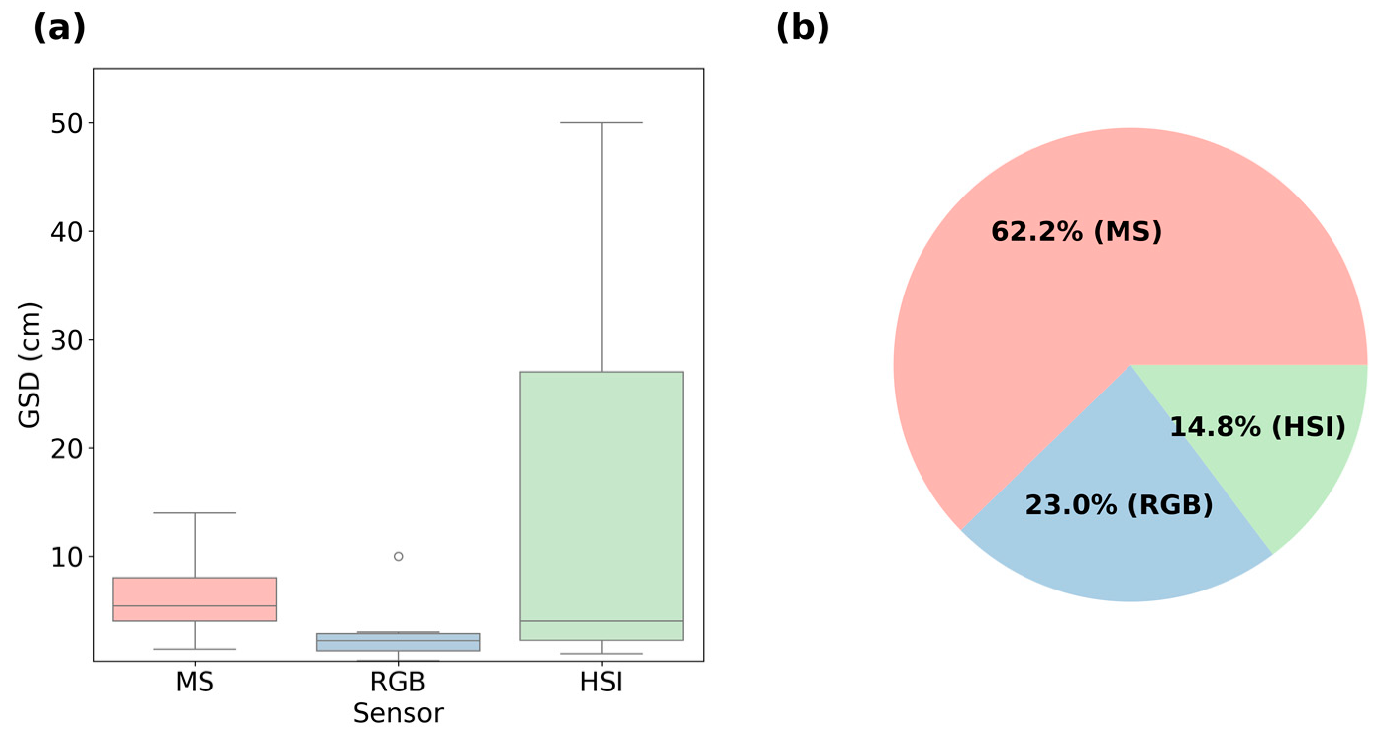
3.3. Specifications and Ground Sampling Distance (GSD)

The utility and effectiveness of UASs in the assessment of NUE related traits are largely dependent upon the type of sensor deployed. Our comprehensive analysis of 45 pertinent research studies reveals the trends and specificities of sensor types, their frequency of usage, and corresponding Ground Sampling Distance (GSD). Here, we outlined the landscape of sensor selection by examining their functional attributes and correlating them with GSD values to discuss their suitability for various scenarios (shown in Figure 5).
MS sensors dominate the field, accounting for 62.3% of total sensor deployments, making them the predominant choice for NUE studies [46]. MS sensors typically capture light across a few visible and near infrared spectral bands at discrete wavelengths [47], and to a lesser extent use the Mid Infrared (MIR) or Thermal Infrared (TIR) bands [48]. The versatility of MS sensors extends their utility across a broad array of traits that indirectly relate to NUE. For example, they have been used for evaluating biomass [49], PNC [50], yield [30], and Plant Nitrogen Uptake (PNU) [51]. Additionally, these sensors are instrumental in measuring key NUE indicators such as the NNI [52], the PFP [46], and the NUtE [10]. Therefore, MS sensors offer a comprehensive toolkit for assessing a wide range of variables that contribute to a more holistic understanding of NUE traits. Meanwhile, GSD of MS balances between image detail and spectral resolution, making them versatile for characterizing N related traits.
Accounting for 23% of sensor usage in the reviewed studies, RGB sensors are typically employed for applications requiring high spatial resolution. RGB sensors have shown effectiveness in predicting NNI [29], PNC, PNU [34], and measuring plant height [36], which is linked to N uptake and NUE. However, their limited spectral bands makes them best suited for studies that emphasize spatial detail (e.g., ground cover) rather than for in-depth research requiring extensive spectral data [28].
HSI sensors, notable for their exceptional spectral qualities and constituting 14.8% of sensor usage, provide data in large volume and complexity. This necessitates advanced analysis methods, often incorporating machine learning and specialized software, to handle the data’s high dimensionality [53,54]. As analytical techniques for HSI data have advanced, there has been a surge in studies using HSI with UAVs for assessing plant NUE, particularly in the recent years of 2022 and 2023, examining indicators like NNI [55,56], NUtE [10,37], and NBI [57].
Selecting the ideal sensor for NUE evaluation depends on the specific goals and conditions of the research. MS sensors are currently favored for their balance between spectral and spatial resolution, suitable for a broad range of NUE studies. However, sensor technology is evolving, with machine learning and AI potentially revolutionizing NUE research. Anticipated advancements may combine the spatial accuracy of RGB sensors with the comprehensive spectral data of HSI sensors through data and sensor fusion. The fusion of advanced analytics with emerging sensor technology promises to refine NUE mapping precision and align with sustainable resource management goals.

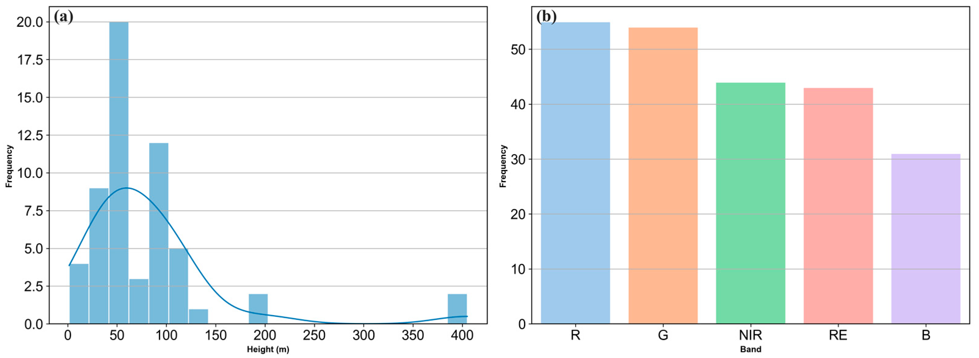
3.4. Flight Parameters and Spectral Characteristics

In the realm of UAV-based remote sensing for NUE assessment, flight height significantly impacts data acquisition and interpretation. Within the scope of this review, the minimum flight height was recorded at 1.5 m above the canopy [58], aimed at optimizing UAV-based data collection for winter wheat growth and nitrogen indicators (shown in Figure 6). The median flight height across reviewed studies approximated 60 m, optimally balancing spatial resolution and area coverage. This median elevation, in synergy with sensor-specific GSD, governs the spatial resolution essential for capturing plant traits variations.
For heights below 100 m, high resolution imagery is emphasized, making it ideal for studies focused on individual plants or small agricultural plots. This range is predominantly the operational domain for RGB sensors, which excel in capturing high-resolution color data. Conversely, moderate heights between 100 and 300 m offer a balanced GSD conducive for MS sensors, thereby extending their applicability to diverse agricultural predictions. HSI sensors are generally deployed at elevations exceeding 300 m to capture a comprehensive spectral range according to the studies included in this review [37]. Although higher heights minimize data variance due to short-term atmospheric changes, such as cloud cover, they often compromise spatial resolution, signified by elevated GSD values.
Spectral band selection plays a critical role in NUE evaluation. Prominent bands include Red (620–750 nm), Green (495–570 nm), Near-Infrared (NIR) (780–1000 nm), and Red-Edge (RE) (680–730 nm). The Red and NIR bands are integral to indices like the Normalized Difference Vegetation Index (NDVI) [31,49], correlating strongly with variables such as leaf nitrogen content [49], biomass [59], and LAI [60]. The Green band is frequently utilized in combination with Red and NIR bands for assessing early plant vigor [61], providing valuable information related to greenness and chlorophyll [18]. The RE band is sensitive to chlorophyll concentration [62]. In this band, the absorption of light by chlorophyll drops sharply, while the scattering of light by the plant’s cellular structure increases. This abrupt transition makes the RE band highly sensitive to variations in chlorophyll concentration [62]. The Blue band is comparatively underutilized owing to its limited canopy penetration and lower reflectance values, making it less suitable for distinguishing plant nitrogen status [63].
In summary, flight height and spectral band selection are not uniform considerations but are influenced by many factors such as research objectives and computational capacities. A harmonized approach to these variables ensures the efficacy of UAV-based remote sensing in NUE assessment. MS sensors, with their balanced GSD and spectral capabilities, emerge as the most pragmatic choice due to their versatility in capturing a range of spectral information while maintaining a reasonable spatial resolution. The MS bands present a spectrum of opportunities for formulating relevant vegetation indices strongly correlated with NUE. Thus, an intricate understanding of these inter-related parameters is pivotal for researchers in tailoring UAV-based remote sensing experiments for NUE evaluation.

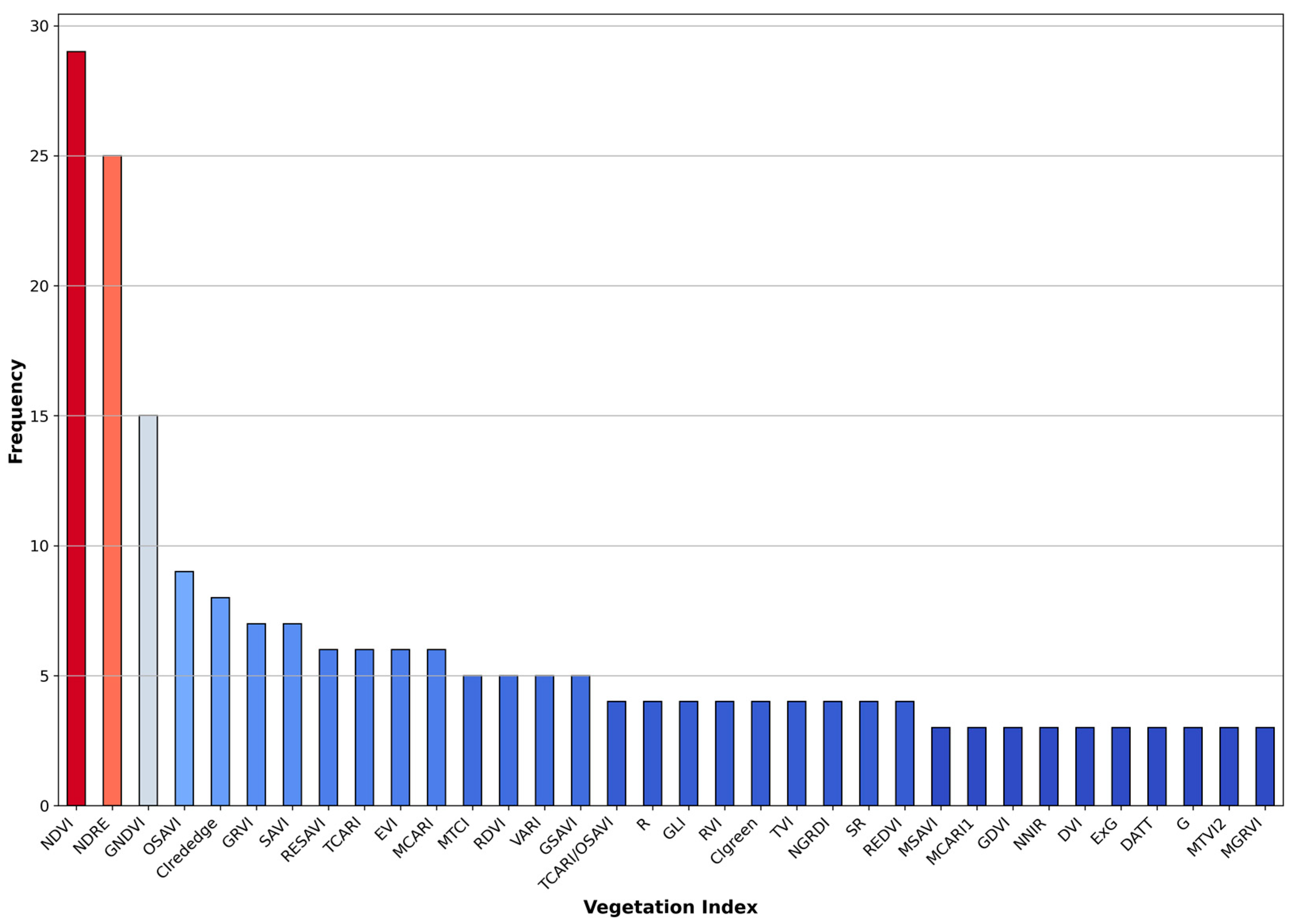
3.5. Commonly Used Vegetation Indices in NUE Assessment

Vegetation indices provide a simplified yet precise method for evaluating essential agronomic parameters by reducing complex spectral data to easily interpretable metrics [44]. Evaluating vegetation indices necessitates careful consideration of factors such as saturation thresholds, sensitivity to plant attributes, growth stage-specific applicability, canopy architecture, and environmental influences [64]. In this review, the NDVI and the Normalized Difference Red Edge (NDRE) were identified as the two most frequently used vegetation indices (Figure 7). NDVI, which uses the Red and NIR bands, is a versatile, general-purpose index sensitive to various plant attributes. However, in high biomass conditions, NDVI tends to saturate. This happens because chlorophyll almost completely absorbs the red light, while the leaf cell structure primarily scatters the NIR light [65]. NDVI saturation can limit its effectiveness in dense vegetation, as the index may not reflect additional biomass or nitrogen content beyond a certain leaf area density. Beyond a certain threshold of leaf area or canopy cover [60], NDVI becomes less sensitive to subtle variations of the canopy. In contrast, NDRE uses the Red Edge and NIR bands and is particularly sensitive to variations associated with plant N trait [66,67]. Additionally, Green Normalized Difference Vegetation Index (GNDVI) incorporates the green band along with the NIR band and is commonly used for early plant vigor assessment [68]. It is less prone to saturation compared to NDVI and usually has strong relation with dry matter [66], NNI [49], and aNUE [17].
The Chlorophyll Index (CI) is commonly calculated using various spectral bands, specifically the Red Edge and Green bands. These variations give rise to different forms of the index, namely the Chlorophyll Index in the Red Edge (CI Red Edge) and the Chlorophyll Index with Green (CI Green). CI Red Edge has been found had a higher estimation accuracy for NNI [47] and nitrogen content than CI Green [66]. For example, CI Red Edge is generally more sensitive to changes in chlorophyll concentration [69], making it suitable for assessing N deficiency-associated chlorophyll change.
Similarly, the Green Ratio Vegetation Index (GRVI) is tailored to chlorophyll concentration and serves as a dependable index for evaluating both plant health and nitrogen status. It has a good performance when estimate AGB, NNI, and PNU [70].
In addition to the aforementioned VIs, indices such as Soil-Adjusted Vegetation Index (SAVI), RESAVI: Red Edge Soil Adjusted Vegetation Index (RESAVI), Optimized Soil-Adjusted Vegetation Index (OSAVI), Transformed Chlorophyll Absorption in Reflectance Index (TCARI), Visible Atmospherically Resistant Index (VARI), and Enhanced Vegetation Index (EVI) also provide unique advantages in UAV-based remote sensing for NUE assessment. For instance, SAVI, RESAVI, and OSAVI minimize soil background influences [71,72], making them ideal for regions with sparse vegetation. Even when the vegetation is not dense, SAVIs provide more accurate estimates of vegetation attributes like biomass [73] and LAI [74]. TCARI is often used in combination with OSAVI to form the TCARI/OSAVI ratio, which further enhances its ability to estimate N related traits [75]. Additionally, VARI was designed to work with standard RGB imagery, eliminating the need for NIR or Red Edge bands [76]. While this makes the index accessible and easy to implement, it does come with limitations in its ability to detect subtle variations in plant health or nutrient status. This is because VARI does not incorporate NIR or Red Edge bands, which are typically sensitive to these plant/canopy structural attributes. Therefore, the index is most suitable for broader assessments focusing on overall vegetation cover rather than detailed evaluations of physiological traits [77]. Lastly, EVI developed for satellite remote sensing has been also employed for UAV-based nitrogen use efficiency assessments [31] and gained significant attention recently [78,79]. Because it incorporates the blue band to correct for atmospheric influences and includes a soil adjustment factor to account for the effects of the ground surface beneath the vegetation, it is less sensitive to atmospheric conditions and background soil variations compared to NDVI [80].
In the context of UAV-based NUE assessment, Modified Triangular Vegetation Index 2 (MTVI2), Simple Ratio (SR), Excess Green Index (ExG), Modified Soil-Adjusted Vegetation Index (MSAVI), and Modified Green Ratio Vegetation Index (MGRVI) are used less frequently when compared to other VIs in UAV-based remote sensing for NUE assessment. Several factors contribute to their less frequent usage. For example, MTVI2 is specifically engineered for extracting the LAI [81] unless it is combined with Modified Chlorophyll Absorption in Reflectance Index (MCARI) to form the MCARI/MTVI2 ratio [32]. The SR index has variations such as Simple Ratio-Red Edge (SR-RE) and Simple Ratio-Near Infrared (SR-NIR), which focus on the Red Edge and near-infrared bands, respectively. Notably, SR-RE has been shown to have a stronger correlation with dry matter compared to SR-NIR [82]. However, the use of only two spectral bands in the SR index limits its capacity to capture the complexity and diversity of vegetation physiology and lacks the soil adjustment features like SAVI or OSAVI [83]. ExG, which is commonly applied in RGB is designed to maximize the response to green vegetation but may not be as sensitive to other plant attributes such as NNI [34,84]. MSAVI and MGRVI are variations of existing indices and might be overshadowed by their more established counterparts [59].
The current landscape of vegetation indices in precision agriculture is marked by a dynamic interplay between established and emerging indices. As UAV technology and spectral analysis methods progress, we anticipate a diversification in the suite of VIs applied to assessments of various functional types of variables related to NUE. This expansion will likely include both traditional indices, prized for their reliability, and innovative indices, which may offer tailored insights for specific crop types, cropping system conditions (e.g., mixed and diversified cropping) and developmental stages (e.g., phenology). Such an evolution is pivotal for the advancement of precision crop management, where the goal is to achieve an optimal balance between N resource inputs and crop yield and quality and ultimately optimal NUE from field to global scale.

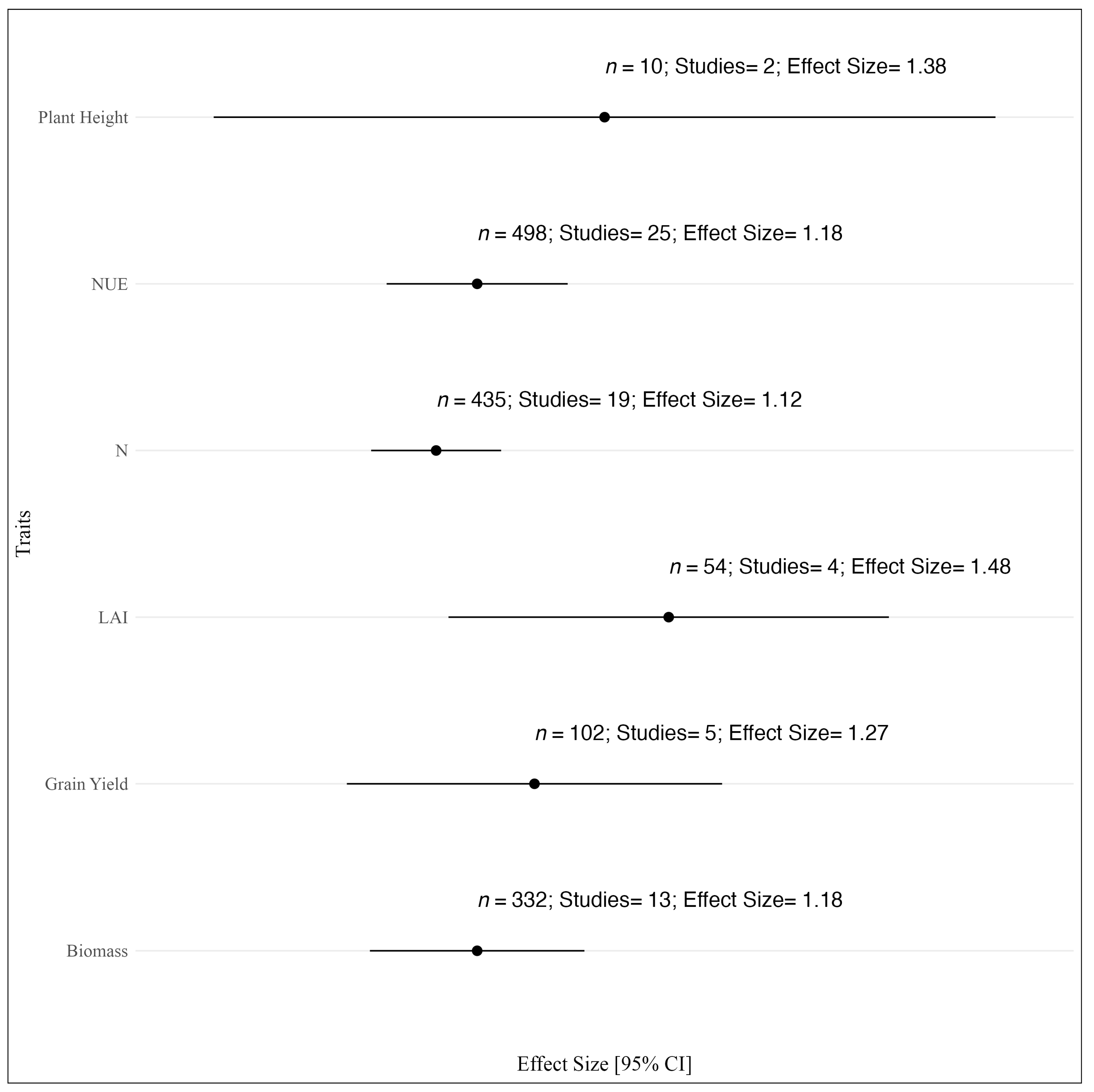
3.6. UAV-Based Trait Estimation for NUE Analysis

Using mixed-effects models, we discerned that the positive aggregate effect sizes for these traits ranged between 1.12 and 1.48, a trend distinctly illustrated in Figure 8. Intriguingly, certain traits, namely Plant Height, LAI, and Grain Yield, despite their biological relevance, found limited representation in extant literature. This limited number of studies for these traits has led to broader confidence intervals, suggesting caution when interpreting these results due to potential sample bias. Consequently, in our analytical approach, we adopted a conservative stance, eschewing exhaustive performance analysis for these traits, details of which are elaborated in Tables S1–S3 and Figures S1–S3 (Supplementary Materials).
Traits that have been extensively studied, such as NUE and biomass, exhibited robust predictive performances, each with an effect size of 1.18. Relatively, the nitrogen content, despite its fundamental biological relevance, displayed a slightly more modest model effect size, pegged at 1.12.
Linear mixed model results underscore the significant influence of sensor type and signal processing technique on the accuracy of predicting NUE related plant traits including nitrogen (Table 1, Figure 9), NUE (Table 2, Figure 10), and biomass (Table 3, Figure 11). The sensor type showed a pronounced difference in the effect on the three traits, with F-statistics of 71.704 for N, 5.256 for NUE, and 18.311 for biomass, reflecting its critical role in the predictive modeling. The data elucidates that single sensor applications, such as HSI, significantly influence the nitrogen trait detection (Estimate = 1.395, SE = 0.174, p < 0.001). HSI’s broad spectral range capture detailed information of plant canopy reflectance across numerous wavelengths, enabling precise detection of nutrient content [85], grain yield [85], LAI [56], and NUE [86].
Notably, the integration of HSI with LiDAR sensors further enhance the model’s predictive capability for NUE (Estimate = 1.152, SE = 0.187, p < 0.001). LiDAR’s ability to generates high resolution three-dimensional structural information complements HSI’s spectral data, enabling a more comprehensive assessment of crop phenotypes [85]. While RGB sensors provide a high resolution imagery, MS sensors extend beyond the visible spectrum, offering insights into plant stresses [79] and photosynthetic efficiency [56]. As a result, the fusion of RGB and MS sensors yields a significant estimate (Estimate = 1.18, SE = 0.14, p < 0.001), suggests an effective strategy for enhancing data richness. Furthermore, implementing thermal sensors, despite a modest effect in isolation (Estimate = 0.216, SE = 0.186, p = 0.266), their utility increase when combined with other sensors [85]. These sensors can detect subtle canopy temperature changes [87], indicative of water stress [12], thus adding a critical dimension to the sensor spectrum and potentially improving the accuracy of trait estimation.
In the case of crop type, the variance of effect is less pronounced, with F-statistics of 0.515 for Nitrogen and 0.501 for NUE, which are lower than those for sensor type. This suggests that while the crop type does influence model predictions, its impact is small compared to the sensor used for data collection. This variation may be rooted in physiological differences between C3 and C4 crops. The C4 photosynthetic pathway is an advanced mechanism that allows plants to more efficiently capture carbon dioxide and utilize nitrogen, particularly under conditions of high light intensity [88], high temperatures [89], and dryness [90]. As a result, C4 crop (i.e., maize) may exhibit a lower leaf nitrogen content (Estimate = 1.176, SE = 0.209, p < 0.001) than some C3 crops (i.e., cotton (Estimate = 2.005, SE = 0.413, p < 0.001) and rice (Estimate = 1.288, SE = 0.123, p < 0.001)), which uses a more common form of photosynthesis that is typically less efficient under warm, dry conditions due to a process called photorespiration [91]. Besides, C4 crops typically show higher NUE, as they can produce more biomass per unit of nitrogen absorbed [92].
Surprisingly, the signal processing techniques manifest even greater variability, with exceptionally high F-statistics, particularly in biomass estimation (F = 65.225), suggesting that the selection of an appropriate technique is paramount for model performance. Physical model-based techniques significantly elevated nitrogen estimation accuracy (Estimate = 2.005, SE = 0.401, p < 0.001). However, the high standard error (SE = 0.401) underscores the need for accurate field measurements to refine these complex simulations. Compared with Multivariate Linear (Estimate = 1.233, SE = 0.069, p < 0.001) and Multivariate Non-Linear regressions (Estimate = 1.344, SE = 0.067, p < 0.001), the relatively simpler univariate regressions appear to have limited predictive power (Estimate = 0.886, SE = 0.06, p < 0.001) in nitrogen estimation. The intricate interactions between spectral data and physiological plant traits, often non-linear, are deftly handled by multivariate non-linear techniques such as random forests [93], support vector machine [72], and extreme learning machine [94]. These machine learning approaches have a pronounced impact on the assessment of both NUE (Estimate = 1.427, SE = 0.082, p < 0.001) and biomass (Estimate = 1.478, SE = 0.125, p < 0.001), showcasing their potential in modeling complex biological processes integral to nutrient efficiency.
Lastly, growth stage demonstrates moderate influence, with F-statistics of 6.295 for Nitrogen and 5.871 for NUE, indicating that phenological stages of the crops have a differential impact on the trait predictions. For nitrogen estimation, compared with early growth stage (Estimate = 0.995, SE = 0.138, p < 0.001), both mid stage (Estimate = 1.085, SE = 0.061, p < 0.001) and late stage (Estimate = 1.093, SE = 0.078, p < 0.001) showed a more significant influence, reflecting the continued relevance of nitrogen during the reproductive phases of plant development. In the context of NUE, it was unexpected to observe that the early stage showed a high estimate accuracy (Estimate = 1.348, SE = 0.102, p < 0.001), followed by the late stage (Estimate = 1.254, SE = 0.086, p < 0.001). The higher estimation accuracy for NUE at the early growth stages may be attributed to the pivotal role that initial nitrogen assimilation plays in setting the foundation for plant health and development [95]. Proficient nitrogen utilization during the early stages is often indicative of a robust root system establishment [96] and vigorous foliar growth [95], which are both vital elements for sustained nutrient absorption and utilization over the plant’s lifecycle [97].
The I C C and the proportions of variance at the study level R 2 2 and at the review dataset level R 3 2 are indicators of heterogeneity. The I C C for sensor type in nitrogen estimation is quite high ( I C C = 0.423), suggesting that the variations within the sensor types are substantial and that there is a high degree of heterogeneity in how different sensors capture information relevant to N content. In contrast, the I C C for crop type in nitrogen estimation is relatively lower ( I C C = 0.144), indicating that the variability in nitrogen content attributable to differences among crop species is less pronounced when compared to sensor types. In the context of NUE, the I C C for sensor type (0.618), crop (0.639), growth stage (0.629), signal processing technique (0.67), and R 2 type (0.604) are uniformly high, which underscores the complexity of NUE as a trait and its sensitivity to a variety of agricultural and methodological conditions. To improve accuracy, NUE modeling must consider a multi-dimensional approach that integrates these diverse but influential factors.
Our analysis demonstrates that the spectral resolution and range of sensor types are crucial for the accurate prediction of biomass and nitrogen content, with HSI sensors being particularly effective due to their wide spectral coverage. The fusion of sensor technologies, notably HSI combined with LiDAR and Thermal imaging, provide enhanced prediction capabilities by integrating structural and temperature data with spectral information. Our analysis reveals that C4 plants like maize exhibit lower leaf nitrogen content but higher NUE and biomass productivity under optimal conditions. This implies the need to consider crop-specific physiological traits in nutrient management strategies for optimal productivity. Signal processing techniques show significant variability in their influence on trait prediction, with physical model-based techniques providing the highest accuracy in nitrogen estimation. The intricate interactions between spectral data and physiological plant traits are often non-linear and can be effectively captured by multivariate non-linear techniques such as machine learning algorithms, which outperform univariate and linear multivariate techniques in both NUE and biomass predictions. Growth stage significantly influences nitrogen estimation accuracy, with early growth stages offering crucial insights on plant health and vigor that is predictive of overall NUE. Early-stage data is particularly valuable, indicating that initial nitrogen assimilation strongly predicts subsequent plant productivity. Finally, the R 2 types, both calibration and validation, are critical in model assessment. Although high calibration R 2 values suggest a good model fit, they also warrant caution against overfitting, underscoring the importance of validation R 2 as a measure of the model’s ability to generalize across different studies.

4. Challenges and New Opportunities for UAV Remote Sensing in NUE

4.1. Accounting for the Effects of Phenological Variations on Spectral Data and Indicators of NUE

Growth stages are pivotal in determining the development of plant traits, particularly NUE, which is closely linked with nitrogen-related traits. Our analysis reveals that the early growth stage offers the highest accuracy in NUE estimation. This stage is characterized by intensive activities such as protein synthesis [39], cell proliferation [98], chlorophyll production for photosynthesis [45], and the synthesis of genetic materials such as DNA and RNA [99], alongside root expansion and enhanced sunlight absorption [100]. These processes are nitrogen-intensive, underlining the essential role of nitrogen in supporting rapid growth and high nutrient uptake, including the synthesis of chlorophyll and other growth-related activities. The correlation between chlorophyll and nitrogen content during this phase facilitates precise predictions of nitrogen-related characteristics via remote sensing, leveraging the spectral signatures of chlorophyll indicators of the plant’s nitrogen status.
However, as plants advance to the reproductive stage, a notable shift occurs. The plant’s nitrogen content may decrease as the plant diverts energy towards seed production [101], leading to a diminished correlation between chlorophyll and nitrogen content. This change can be attributed to several factors, including a physiological shift from leaf development to reproduction, nutrient reallocation within the plant, and the impact of environmental stresses on nutrient uptake or chlorophyll synthesis. Consequently, the predictive accuracy for nitrogen through remote sensing declines in later growth stages, as spectral indicators become less representative of the plant’s nitrogen content. Additionally, factors such as LAI, canopy structure, and soil background vary between growth stages and can alter spectral signatures, further complicating accurate predictions of remote sensing in estimating plant traits.
The vegetative stage is thus revealed as a critical period for analysis. During this phase, plants exhibit their most dynamic growth, with increased chlorophyll content leading to lower red reflectance in the visible spectrum. This spectral behavior, alongside rising LAI and a dynamic canopy structure [102], not only highlights the plant’s vigorous growth and elevated nitrogen demand [103] but also presents an opportune and challenging time window for breaking down canopy spectral data into individual traits related to NUE while eliminating the confounding effects of phenology. As the plant transitions into the reproductive stage, physiological and spectroscopic profiles evolve [104]. Leaf chlorophyll and nitrogen declines are asynchronous in both time point and magnitude, increasing the complexity of attributing canopy spectral patterns to individual traits, such as the extent to which the canopy spectral increase is due to nitrogen remobilization from senescing leaves to developing reproductive parts.

4.2. Correcting Canopy Structural Effects on UAV-Derived NUE Estimates

The structural characteristics of the canopy, such as leaf density and orientation, directly influence the absorption and reflection of light across different spectral bands, thereby affecting the spectral signatures captured by UAV-based sensors [105,106]. Notably, the canopy structure significantly modulates the spectral signatures detectable through UAV remote sensing, making it critical to consider canopy structural variations when gleaning insights on NUE of plant health [107,108].
Wheat canopies can be characterized by four main structural types based on the orientation and disposition of their leaves, including horizontally spreading type, erect type, semierect type, and mixed type [109]. The horizontally spreading type is characterized by leaves that predominantly lie flat, parallel, or nearly so to the ground. This type of canopy maximizes light interception when sunlight is abundant throughout the day [110]. Spectrally, this orientation yields consistent readings, though areas interposed between leaves might exhibit shadow effects, potentially attenuating reflectance [111]. Conversely, the Erect Type presents leaves that are oriented almost perpendicularly, facilitating sunlight to permeate deeper layers, a trait beneficial for promoting photosynthesis in densely cultivated areas [112]. This varied leaf orientation introduces a degree of spectral variability due to complex interactions between light and the canopy. With sunlight striking leaves at different angles, this orientation enhances multiple scattering, characterized by photons undergoing several interactions with the canopy before they are reflected. The captured spectral signatures can change based on the time of day or the position of the sensor, leading to potential inconsistencies in the data [113]. The Semi-erect Type, situated between the other canopy orientations, represents an intermediate type of leaf angle distributions. Its distinct canopy structure is neither fully flat nor completely upright. The canopy’s mixed orientations can lead to varied spectral responses and create nuances that introduce unique challenges in image preprocessing due to the interplay of light conditions and spatial heterogeneity within the canopy [114]. In contrast, the mixed type is characterized by a more diverse blend of leaf orientations. This multifaceted structure further intensifies the complexity, as the canopy encompasses a spectrum of light interactions, ranging from deep penetrations to significant shadowing effects [115].
In summary, to enhance the accuracy of UAV-based NUE assessments, it is imperative to correct canopy structure effects on spectral variability for predicting N content. This is because the multiple scattering of photons due to leaf and canopy 3D arrangement complicates reflectance, necessitating corrections for accurate foliar nitrogen content interpretation. Canopy structures vary from horizontally spreading to erect types, each with unique light absorption and reflection patterns, posing challenges in spectral analysis. The implementation of advanced preprocessing methods such as BRDF corrections is crucial [116]. These methods account for the leaf orientation and density-related spectral effects by normalizing reflectance data to a standard geometrical perspective, thus minimizing the variability caused by different viewing angles or solar positions. By incorporating these corrections, we can reduce the confounding spectral influences of canopy structure, ensuring that the variability in the data reflects actual differences in N rather than artifacts of how light interacts with the canopy. This approach enhances the precision of the translation of remote sensing data to biologically meaningful variables and leading to more reliable interpretations.

4.3. Advancing Remote Sensing through Imagery Data Fusion and AI-Driven Feature Analysis

In the domain of remote sensing, the integration of data from various sensor technologies is a critical process, referred to as feature fusion. This methodology harnesses the inherent strengths of each data compilation, maintaining their full dimensionality to offer an expansive and nuanced perspective on the analyzed phenomena [64]. To date, the majority of work employing multiple sensors take advantage of data integration rather than data fusion [117,118,119], especially imagery data fusion. Different from data integration, data fusion extends this paradigm by engaging in both the integration and condensation of data, which can enhance efficiency and accuracy in representation. For instance, Jie et al. adeptly used data fusion through the upscaling of UAV-derived maps to reconcile with the coarser spatial resolution inherent in satellite imagery. This approach resulted in a synthesized data compilation with an augmented predictive capacity and elevated confidence in model output, demonstrating an efficacious reduction of data sets with enriched analytical value [93]. Additionally, Canh et al. employed a sophisticated deep learning approach utilizing convolutional neural networks (CNNs) to process a composite of hyperspectral, thermal, and LiDAR imagery. Their method transcended simple data integration by reducing the overall data volume, thus amplifying the predictive power of the model and refining the insights gained [85]. These data fusion techniques unify disparate data forms to forge a composite analytical lens that markedly elevates the understanding and prediction of phenotypic attributes.
The advent of Artificial Intelligence (AI) in remote sensing has propelled data fusion methodologies to the forefront [120], especially with the use of Machine Learning (ML) [121] and Deep Learning (DL) algorithms [122]. CNNs adeptly process grid-like data from multispectral and hyperspectral images [120,123], while Random Forest (RF) algorithms, with their robustness to overfitting, expertly integrate UAV and satellite data to predict environmental variables [124,125]. Moreover, the SVMs, RNNs, LSTM networks, Autoencoders, and GNNs each contribute uniquely to the fusion process, whether by mapping complex land cover classifications or capturing temporal dynamics in satellite time-series data [126,127,128,129], thereby facilitating continuous monitoring and forecasting of ecological changes.
As mentioned in the previous section, the complexity of canopy structure poses challenges to spectral analysis. While Texture Features (TFs) enrich spectral data analysis by providing additional context, enabling differentiation between crops with similar spectral profiles but distinct structural characteristics [130]. The incorporation of TFs into data fusion processes addresses the complexities of interpreting intricate canopy structures. Advanced image analysis methods, including GLCM [131] and LBP [132], elucidate the nuanced spatial arrangements within the canopy, offering enhanced classification accuracy and aiding in the distinction of spectrally analogous but structurally diverse canopies [133]. The integration of TFs with spectral data through advanced AI-driven algorithms like CNNs, and supported by preprocessing strategies like BRDF corrections, represent the next frontier in data fusion. Such integrative approaches not only consolidate information from a broad spectrum of sources but also significantly refine the interpretability and utility of the resultant models.
This holistic perspective underscores the importance of sophisticated data fusion in overcoming the challenges of remote sensing, specifically in agricultural contexts where the accurate phenotyping of crop traits for improved resource use efficiency. As the remote sensing field evolves, the impetus to harness the full potential of data fusion becomes increasingly pivotal, promising to unravel the complexities of crop growth and health in an ever-changing global environment.

5. Conclusions

UASs have significantly impacted the landscape of modern agriculture, serving as crucial instruments in offering granular insights into plant health, growth, and NUE. This review sheds light on the factors influencing UAV assessments of N status and N use efficiency. These range from plant attributes, such as growth stages and canopy structures, to technical aspects like sensor calibrations and flight parameters.
The incorporation of TFs in data analysis represents a pivotal advancement, enabling more detailed and accurate canopy assessments. These features provide a detailed view of the plant canopy’s micro-architecture. They enhance the information gained from spectral data and offer a more accurate interpretation, particularly in cases where traditional spectral indices are not sufficient. Furthermore, in an era where agriculture faces challenges like sustainability, changing climate patterns, dwindling resources, and the ever-growing demand for increased productivity, the role of UASs becomes indispensable. Their ability to provide timely high-resolution data is invaluable, but the real potential lies in integrating UAV-derived insights with data from other sensing platforms and scales. This multimodal integration could potentially provide a comprehensive, multi-scale view of agricultural landscapes, thereby enabling more informed decisions and effective interventions.
In the future, as the nexus between technology and agriculture deepens, UAVs, fortified by advanced analytical methodologies and Artificial Intelligence (AI), are poised to be at the forefront of precision farming. These technologies, when applied judiciously and integrated seamlessly with other data sources, hold the promise of transforming current agricultural practices to more productive and resource-efficient ones.

Supplementary Materials

The following supporting information can be downloaded at: https://www.mdpi.com/article/10.3390/rs16050838/s1, Figure S1: Observed Fisher’s Z effect sizes with their 95% confidence interval for Grain Yield; Figure S2: Observed Fisher’s Z effect sizes with their 95% confidence interval for Leaf Area Index; Figure S3: Observed Fisher’s Z effect sizes with their 95% confidence interval for Plant Height; Table S1: Regression models without moderator (Null) and with one moderator (Sensor Type, Crop, Signal Processing Technique, Growth Stage, R 2 Type, respectively) for Plant Height; Table S2: Regression models without moderator (Null) and with one moderator (Sensor Type, Crop, Signal Processing Technique, Growth Stage, R 2 Type, respectively) for Grain Yield; Table S3: Regression models without moderator (Null) and with one moderator (Sensor Type, Crop, Signal Processing Technique, Growth Stage, R 2 Type, respectively) for Leaf Area Index. Appendix S1: Qualitatively analysis and quantitatively analysis; Appendix S2: Engine search.

Author Contributions

Conceptualization, J.Z. and K.Y.; methodology, J.Z.; software, J.Z.; validation, J.Z. and K.Y.; formal analysis, J.Z.; investigation, J.Z.; resources, K.Y.; data curation, J.Z.; writing—original draft preparation, J.Z.; writing—review and editing, Y.H., F.L., K.G.F. and K.Y.; visualization, J.Z.; supervision, K.Y. All authors have read and agreed to the published version of the manuscript.

Funding

This research has been partly supported by the AmAIzed project funded by AgroMissionHub.

Data Availability Statement

Data are contained within the article and Supplementary Materials.

Acknowledgments

Special thanks to Haibo Yang for his invaluable support during the initial stages of this review. His insights were crucial and significantly contributed to its successful completion.

Conflicts of Interest

The authors declare no conflicts of interest.

References

  1. Anas, M.; Liao, F.; Verma, K.K.; Sarwar, M.A.; Mahmood, A.; Chen, Z.-L.; Li, Q.; Zeng, X.-P.; Liu, Y.; Li, Y.-R. Fate of nitrogen in agriculture and environment: Agronomic, eco-physiological and molecular approaches to improve nitrogen use efficiency. Biol. Res. 2020, 53, 47. [Google Scholar] [CrossRef]
  2. Ahmed, M.; Rauf, M.; Mukhtar, Z.; Saeed, N.A. Excessive use of nitrogenous fertilizers: An unawareness causing serious threats to environment and human health. Environ. Sci. Pollut. Res. 2017, 24, 26983–26987. [Google Scholar] [CrossRef] [PubMed]
  3. EU Nitrogen Expert Panel. Nitrogen Expert Panel. Nitrogen Use Efficiency (NUE). In An Indicator for the Utilization of Nitrogen in Agriculture and Food Systems; Wageningen University: Wageningen, The Netherlands, 2015. [Google Scholar]
  4. Li, Y.; Li, B.; Yuan, Y.; Liu, Y.; Li, R.; Liu, W. Improved soil surface nitrogen balance method for assessing nutrient use efficiency and potential environmental impacts within an alpine meadow dominated region. Environ. Pollut. 2023, 325, 121446. [Google Scholar] [CrossRef] [PubMed]
  5. Scheer, C.; Rowlings, D.W.; Antille, D.L.; De Antoni Migliorati, M.; Fuchs, K.; Grace, P.R. Improving nitrogen use efficiency in irrigated cotton production. Nutr. Cycl. Agroecosyst. 2023, 125, 95–106. [Google Scholar] [CrossRef]
  6. Stahl, A.; Friedt, W.; Wittkop, B.; Snowdon, R.J. Complementary diversity for nitrogen uptake and utilisation efficiency reveals broad potential for increased sustainability of oilseed rape production. Plant Soil 2016, 400, 245–262. [Google Scholar] [CrossRef]
  7. Wan, X.; Wu, W.; Shah, F. Nitrogen fertilizer management for mitigating ammonia emission and increasing nitrogen use efficiencies by 15N stable isotopes in winter wheat. Sci. Total Environ. 2021, 790, 147587. [Google Scholar] [CrossRef]
  8. Han, L.; Yang, G.; Dai, H.; Xu, B.; Yang, H.; Feng, H.; Li, Z.; Yang, X. Modeling maize above-ground biomass based on machine learning approaches using UAV remote-sensing data. Plant Methods 2019, 15, 10. [Google Scholar] [CrossRef]
  9. Brinkhoff, J.; Dunn, B.W.; Robson, A.J.; Dunn, T.S.; Dehaan, R.L. Modeling Mid-Season Rice Nitrogen Uptake Using Multispectral Satellite Data. Remote Sens. 2019, 11, 1837. [Google Scholar] [CrossRef]
  10. Hegedus, P.B.; Ewing, S.A.; Jones, C.; Maxwell, B.D. Using spatially variable nitrogen application and crop responses to evaluate crop nitrogen use efficiency. Nutr. Cycl. Agroecosyst 2023, 126, 1–20. [Google Scholar] [CrossRef]
  11. Li, J.-L.; Su, W.-H.; Zhang, H.-Y.; Peng, Y. A real-time smart sensing system for automatic localization and recognition of vegetable plants for weed control. Front. Plant Sci. 2023, 14, 1133969. [Google Scholar] [CrossRef]
  12. Ludovisi, R.; Tauro, F.; Salvati, R.; Khoury, S.; Mugnozza Scarascia, G.; Harfouche, A. UAV-Based Thermal Imaging for High-Throughput Field Phenotyping of Black Poplar Response to Drought. Front. Plant Sci. 2017, 8, 1681. [Google Scholar] [CrossRef]
  13. Zhou, X.; Zheng, H.B.; Xu, X.Q.; He, J.Y.; Ge, X.K.; Yao, X.; Cheng, T.; Zhu, Y.; Cao, W.X.; Tian, Y.C. Predicting grain yield in rice using multi-temporal vegetation indices from UAV-based multispectral and digital imagery. ISPRS J. Photogramm. Remote Sens. 2017, 130, 246–255. [Google Scholar] [CrossRef]
  14. Gašparović, M.; Zrinjski, M.; Barković, Đ.; Radočaj, D. An automatic method for weed mapping in oat fields based on UAV imagery. Comput. Electron. Agric. 2020, 173, 105385. [Google Scholar] [CrossRef]
  15. Zha, H.; Miao, Y.; Wang, T.; Li, Y.; Zhang, J.; Sun, W.; Feng, Z.; Kusnierek, K. Improving Unmanned Aerial Vehicle Remote Sensing-Based Rice Nitrogen Nutrition Index Prediction with Machine Learning. Remote Sens. 2020, 12, 215. [Google Scholar] [CrossRef]
  16. Wahab, I.; Hall, O.; Jirström, M. Remote Sensing of Yields: Application of UAV Imagery-Derived NDVI for Estimating Maize Vigor and Yields in Complex Farming Systems in Sub-Saharan Africa. Drones 2018, 2, 28. [Google Scholar] [CrossRef]
  17. Yang, M.J.; Hassan, M.A.; Xu, K.J.; Zheng, C.Y.; Rasheed, A.; Zhang, Y.; Jin, X.L.; Xia, X.C.; Xiao, Y.G.; He, Z.H. Assessment of Water and Nitrogen Use Efficiencies Through UAV-Based Multispectral Phenotyping in Winter Wheat. Front. Plant Sci. 2020, 11, 927. [Google Scholar] [CrossRef] [PubMed]
  18. Liang, T.; Duan, B.; Luo, X.Y.; Ma, Y.; Yuan, Z.Q.; Zhu, R.S.; Peng, Y.; Gong, Y.; Fang, S.H.; Wu, X.T. Identification of High Nitrogen Use Efficiency Phenotype in Rice (Oryza sativa L.) Through Entire Growth Duration by Unmanned Aerial Vehicle Multispectral Imagery. Front. Plant Sci. 2021, 12, 740414. [Google Scholar] [CrossRef] [PubMed]
  19. Quan, Z.; Zhang, X.; Fang, Y.; Davidson, E.A. Different quantification approaches for nitrogen use efficiency lead to divergent estimates with varying advantages. Nat. Food 2021, 2, 241–245. [Google Scholar] [CrossRef] [PubMed]
  20. Cormier, F.; Foulkes, J.; Hirel, B.; Gouache, D.; Moënne-Loccoz, Y.; Le Gouis, J. Breeding for increased nitrogen-use efficiency: A review for wheat (T. aestivum L.). Plant Breed. 2016, 135, 255–278. [Google Scholar] [CrossRef]
  21. Hawkesford, M.J. Genetic variation in traits for nitrogen use efficiency in wheat. J. Exp. Bot. 2017, 68, 2627–2632. [Google Scholar] [CrossRef]
  22. Van Cleemput, E.; Vanierschot, L.; Fernández-Castilla, B.; Honnay, O.; Somers, B. The functional characterization of grass- and shrubland ecosystems using hyperspectral remote sensing: Trends, accuracy and moderating variables. Remote Sens. Environ. 2018, 209, 747–763. [Google Scholar] [CrossRef]
  23. Finn, G.A.; Straszewski, A.E.; Peterson, V. A general growth stage key for describing trees and woody plants. Ann. Appl. Biol. 2007, 151, 127–131. [Google Scholar] [CrossRef]
  24. Liu, L.; Li, H.; Zhu, S.; Gao, Y.; Zheng, X.; Xu, Y. The response of agronomic characters and rice yield to organic fertilization in subtropical China: A three-level meta-analysis. Field Crops Res. 2021, 263, 108049. [Google Scholar] [CrossRef]
  25. Wang, Y.; Li, Y.; Liang, J.; Bi, Y.; Wang, S.; Shang, Y. Climatic Changes and Anthropogenic Activities Driving the Increase in Nitrogen: Evidence from the South-to-North Water Diversion Project. Water 2021, 13, 2517. [Google Scholar] [CrossRef]
  26. Mastrocicco, M.; Colombani, N.; Soana, E.; Vincenzi, F.; Castaldelli, G. Intense rainfalls trigger nitrite leaching in agricultural soils depleted in organic matter. Sci. Total Environ. 2019, 665, 80–90. [Google Scholar] [CrossRef] [PubMed]
  27. Lu, Y.; Li, P.; Li, M.; Wen, M.; Wei, H.; Zhang, Z. Coupled Dynamics of Soil Water and Nitrate in the Conversion of Wild Grassland to Farmland and Apple Orchard in the Loess Drylands. Agronomy 2023, 13, 1711. [Google Scholar] [CrossRef]
  28. Li, J.W.; Zhang, F.; Qian, X.Y.; Zhu, Y.H.; Shen, G.X. Quantification of rice canopy nitrogen balance index with digital imagery from unmanned aerial vehicle. Remote Sens. Lett. 2015, 6, 183–189. [Google Scholar] [CrossRef]
  29. Schirrmann, M.; Giebel, A.; Gleiniger, F.; Pflanz, M.; Lentschke, J.; Dammer, K.H. Monitoring Agronomic Parameters of Winter Wheat Crops with Low-Cost UAV Imagery. Remote Sens. 2016, 8, 706. [Google Scholar] [CrossRef]
  30. Thompson, L.J.; Puntel, L.A. Transforming Unmanned Aerial Vehicle (UAV) and Multispectral Sensor into a Practical Decision Support System for Precision Nitrogen Management in Corn. Remote Sens. 2020, 12, 1597. [Google Scholar] [CrossRef]
  31. Kefauver, S.C.; Vicente, R.; Vergara-Diaz, O.; Fernandez-Gallego, J.A.; Kerfal, S.; Lopez, A.; Melichar, J.P.E.; Molins, M.D.S.; Araus, J.L. Comparative UAV and Field Phenotyping to Assess Yield and Nitrogen Use Efficiency in Hybrid and Conventional Barle. Front. Plant Sci. 2017, 8, 1733. [Google Scholar] [CrossRef]
  32. Argento, F.; Anken, T.; Abt, F.; Vogelsanger, E.; Walter, A.; Liebisch, F. Site-specific nitrogen management in winter wheat supported by low-altitude remote sensing and soil data. Precis. Agric. 2021, 22, 364–386. [Google Scholar] [CrossRef]
  33. Hu, D.-W.; Sun, Z.-P.; Li, T.-L.; Yan, H.-Z.; Zhang, H. Nitrogen Nutrition Index and Its Relationship with N Use Efficiency, Tuber Yield, Radiation Use Efficiency, and Leaf Parameters in Potatoes. J. Integr. Agric. 2014, 13, 1008–1016. [Google Scholar] [CrossRef]
  34. Song, X.Y.; Yang, G.J.; Xu, X.G.; Zhang, D.Y.; Yang, C.H.; Feng, H.K. Winter Wheat Nitrogen Estimation Based on Ground-Level and UAV-Mounted Sensors. Sensors 2022, 22, 549. [Google Scholar] [CrossRef] [PubMed]
  35. Dong, R.; Miao, Y.; Wang, X.; Chen, Z.; Yuan, F. Improving maize nitrogen nutrition index prediction using leaf fluorescence sensor combined with environmental and management variables. Field Crops Res. 2021, 269, 108180. [Google Scholar] [CrossRef]
  36. Wang, J.; Meyer, S.; Xu, X.; Weisser, W.W.; Yu, K. Drone Multispectral Imaging Captures the Effects of Soil Nmin on Canopy Structure and Nitrogen Use Efficiency in Wheat. Available online: https://ssrn.com/abstract=4699313 (accessed on 18 January 2024). [CrossRef]
  37. Olson, M.B.; Crawford, M.M.; Vyn, T.J. Hyperspectral Indices for Predicting Nitrogen Use Efficiency in Maize Hybrids. Remote Sens. 2022, 14, 1721. [Google Scholar] [CrossRef]
  38. Luo, H.Z.; Dewitte, K.; Landschoot, S.; Sigurnjak, I.; Robles-Aguilar, A.A.; Michels, E.; De Neve, S.; Haesaert, G.; Meers, E. Benefits of biobased fertilizers as substitutes for synthetic nitrogen fertilizers: Field assessment combining minirhizotron and UAV-based spectrum sensing technologies. Front. Environ. Sci. 2022, 10, 988932. [Google Scholar] [CrossRef]
  39. Fageria, N.K.; Baligar, V.C. Enhancing Nitrogen Use Efficiency in Crop Plants. Adv. Agron. 2005, 88, 97–185. [Google Scholar]
  40. Gianquinto, G.; Orsini, F.; Fecondini, M.; Mezzetti, M.; Sambo, P.; Bona, S. A methodological approach for defining spectral indices for assessing tomato nitrogen status and yield. Eur. J. Agron. 2011, 35, 135–143. [Google Scholar] [CrossRef]
  41. Li, W.; Wu, W.; Yu, M.; Tao, H.; Yao, X.; Cheng, T.; Zhu, Y.; Cao, W.; Tian, Y. Monitoring rice grain protein accumulation dynamics based on UAV multispectral data. Field Crops Res. 2023, 294, 108858. [Google Scholar] [CrossRef]
  42. Xu, G.; Fan, X.; Miller, A.J. Plant Nitrogen Assimilation and Use Efficiency. Annu. Rev. Plant Biol. 2012, 63, 153–182. [Google Scholar] [CrossRef]
  43. Guo, X.; He, H.; An, R.; Zhang, Y.; Yang, R.; Cao, L.; Wu, X.; Chen, B.; Tian, H.; Gao, Y. Nitrogen use-inefficient oilseed rape genotypes exhibit stronger growth potency during the vegetative growth stage. Acta Physiol. Plant. 2019, 41, 175. [Google Scholar] [CrossRef]
  44. Bendig, J.; Yu, K.; Aasen, H.; Bolten, A.; Bennertz, S.; Broscheit, J.; Gnyp, M.L.; Bareth, G. Combining UAV-based plant height from crop surface models, visible, and near infrared vegetation indices for biomass monitoring in barley. Int. J. Appl. Earth Obs. Geoinf. 2015, 39, 79–87. [Google Scholar] [CrossRef]
  45. Jia, M.; Colombo, R.; Rossini, M.; Celesti, M.; Zhu, J.; Cogliati, S.; Cheng, T.; Tian, Y.; Zhu, Y.; Cao, W.; et al. Estimation of leaf nitrogen content and photosynthetic nitrogen use efficiency in wheat using sun-induced chlorophyll fluorescence at the leaf and canopy scales. Eur. J. Agron. 2021, 122, 126192. [Google Scholar] [CrossRef]
  46. Liu, J.K.; Zhu, Y.J.; Tao, X.Y.; Chen, X.F.; Li, X.W. Rapid prediction of winter wheat yield and nitrogen use efficiency using consumer-grade unmanned aerial vehicles multispectral imagery. Front. Plant Sci. 2022, 13, 1032170. [Google Scholar] [CrossRef] [PubMed]
  47. Liu, S.S.; Li, L.T.; Gao, W.H.; Zhang, Y.K.; Liu, Y.N.; Wang, S.Q.; Lu, J.W. Diagnosis of nitrogen status in winter oilseed rape (Brassica napus L.) using in-situ hyperspectral data and unmanned aerial vehicle (UAV) multispectral images. Comput. Electron. Agric. 2018, 151, 185–195. [Google Scholar] [CrossRef]
  48. Qian, Y.-G.; Wang, N.; Ma, L.-L.; Liu, Y.-K.; Wu, H.; Tang, B.-H.; Tang, L.-L.; Li, C.-R. Land surface temperature retrieved from airborne multispectral scanner mid-infrared and thermal-infrared data. Opt. Express 2016, 24, A257–A269. [Google Scholar] [CrossRef] [PubMed]
  49. Arroyo, J.A.; Gomez-Castaneda, C.; Ruiz, E.; de Cote, E.M.; Gavi, F.; Sucar, L.E. Assessing Nitrogen Nutrition in Corn Crops with Airborne Multispectral Sensors. In Proceedings of the Advances in Artificial Intelligence: From Theory to Practice (IEA/AIE 2017), PT II, Arras, France, 27–30 June 2017; pp. 259–267. [Google Scholar]
  50. Chen, Z.C.; Miao, Y.X.; Lu, J.J.; Zhou, L.; Li, Y.; Zhang, H.Y.; Lou, W.D.; Zhang, Z.; Kusnierek, K.; Liu, C.H. In-Season Diagnosis of Winter Wheat Nitrogen Status in Smallholder Farmer Fields Across a Village Using Unmanned Aerial Vehicle-Based Remote Sensing. Agronomy 2019, 9, 619. [Google Scholar] [CrossRef]
  51. Zhang, J.Y.; Wang, W.K.; Krienke, B.; Cao, Q.; Zhu, Y.; Cao, W.X.; Liu, X.J. In-season variable rate nitrogen recommendation for wheat precision production supported by fixed-wing UAV imagery. Precis. Agric. 2022, 23, 830–853. [Google Scholar] [CrossRef]
  52. Heinemann, P.; Schmidhalter, U. Spectral assessments of N-related maize traits: Evaluating and defining agronomic relevant detection limits. Field Crops Res. 2022, 289, 108710. [Google Scholar] [CrossRef]
  53. Bernabe, S.; Sanchez, S.; Plaza, A.; Lopez, S.; Benediktsson, J.A.; Sarmiento, R. Hyperspectral Unmixing on GPUs and Multi-Core Processors: A Comparison. IEEE J. Sel. Top. Appl. Earth Obs. Remote Sens. 2013, 6, 1386–1398. [Google Scholar] [CrossRef]
  54. Sánchez, S.; Paz, A.; Martín, G.; Plaza, A. Parallel unmixing of remotely sensed hyperspectral images on commodity graphics processing units. Concurr.Comput. Pract. Exp. 2011, 23, 1538–1557. [Google Scholar] [CrossRef]
  55. Liu, H.Y.; Zhu, H.C.; Li, Z.H.; Yang, G.J. Quantitative analysis and hyperspectral remote sensing of the nitrogen nutrition index in winter wheat. Int. J. Remote Sens. 2020, 41, 858–881. [Google Scholar] [CrossRef]
  56. Du, R.; Chen, J.; Xiang, Y.; Zhang, Z.; Yang, N.; Yang, X.; Tang, Z.; Wang, H.; Wang, X.; Shi, H.; et al. Incremental learning for crop growth parameters estimation and nitrogen diagnosis from hyperspectral data. Comput. Electron. Agric. 2023, 215, 108356. [Google Scholar] [CrossRef]
  57. Wang, L.; Gao, R.; Li, C.; Wang, J.; Liu, Y.; Hu, J.; Li, B.; Qiao, H.; Feng, H.; Yue, J. Mapping Soybean Maturity and Biochemical Traits Using UAV-Based Hyperspectral Images. Remote Sens. 2023, 15, 4807. [Google Scholar] [CrossRef]
  58. Jiang, J.; Zhang, Z.Y.; Cao, Q.; Liang, Y.; Krienke, B.; Tian, Y.C.; Zhu, Y.; Cao, W.X.; Liu, X.J. Use of an Active Canopy Sensor Mounted on an Unmanned Aerial Vehicle to Monitor the Growth and Nitrogen Status of Winter Wheat. Remote Sens. 2020, 12, 3684. [Google Scholar] [CrossRef]
  59. Pereira, F.R.D.; de Lima, J.P.; Freitas, R.G.; Dos Reis, A.A.; do Amaral, L.R.; Figueiredo, G.; Lamparelli, R.A.C.; Magalhaes, P.S.G. Nitrogen variability assessment of pasture fields under an integrated crop-livestock system using UAV, PlanetScope, and Sentinel-2 data. Comput. Electron. Agric. 2022, 193, 106645. [Google Scholar] [CrossRef]
  60. Gong, Y.; Yang, K.; Lin, Z.; Fang, S.; Wu, X.; Zhu, R.; Peng, Y. Remote estimation of leaf area index (LAI) with unmanned aerial vehicle (UAV) imaging for different rice cultivars throughout the entire growing season. Plant Methods 2021, 17, 88. [Google Scholar] [CrossRef] [PubMed]
  61. Vukasovic, S.; Alahmad, S.; Christopher, J.; Snowdon, R.J.; Stahl, A.; Hickey, L.T. Dissecting the Genetics of Early Vigour to Design Drought-Adapted Wheat. Front. Plant Sci. 2021, 12, 754439. [Google Scholar] [CrossRef] [PubMed]
  62. Zheng, T.; Liu, N.; Wu, L.; Li, M.; Sun, H.; Zhang, Q.; Wu, J. Estimation of Chlorophyll Content in Potato Leaves Based on Spectral Red Edge Position. IFAC-PapersOnLine 2018, 51, 602–606. [Google Scholar] [CrossRef]
  63. Kochetova, G.V.; Avercheva, O.V.; Bassarskaya, E.M.; Kushunina, M.A.; Zhigalova, T.V. Effects of Red and Blue LED Light on the Growth and Photosynthesis of Barley (Hordeum vulgare L.) Seedlings. J. Plant Growth Regul. 2023, 42, 1804–1820. [Google Scholar] [CrossRef]
  64. da Costa, M.B.T.; Silva, C.A.; Broadbent, E.N.; Leite, R.V.; Mohan, M.; Liesenberg, V.; Stoddart, J.; do Amaral, C.H.; de Almeida, D.R.A.; da Silva, A.L.; et al. Beyond trees: Mapping total aboveground biomass density in the Brazilian savanna using high-density UAV-lidar data. For. Ecol. Manag. 2021, 491, 119155. [Google Scholar] [CrossRef]
  65. Gu, Y.; Wylie, B.K.; Howard, D.M.; Phuyal, K.P.; Ji, L. NDVI saturation adjustment: A new approach for improving cropland performance estimates in the Greater Platte River Basin, USA. Ecol. Indic. 2013, 30, 1–6. [Google Scholar] [CrossRef]
  66. Wang, H.; Mortensen, A.K.; Mao, P.S.; Boelt, B.; Gislum, R. Estimating the nitrogen nutrition index in grass seed crops using a UAV-mounted multispectral camera. Int. J. Remote Sens. 2019, 40, 2467–2482. [Google Scholar] [CrossRef]
  67. Roy Choudhury, M.; Christopher, J.; Das, S.; Apan, A.; Menzies, N.W.; Chapman, S.; Mellor, V.; Dang, Y.P. Detection of calcium, magnesium, and chlorophyll variations of wheat genotypes on sodic soils using hyperspectral red edge parameters. Environ. Technol. Innov. 2022, 27, 102469. [Google Scholar] [CrossRef]
  68. Singh, S.; Pandey, P.; Khan, M.S.; Semwal, M. Multi-temporal High Resolution Unmanned Aerial Vehicle (UAV) Multispectral Imaging for Menthol Mint Crop Monitoring. In Proceedings of the 2021 6th International Conference for Convergence in Technology (I2CT), Maharashtra, India, 2–4 April 2021; pp. 1–4. [Google Scholar]
  69. Peng, J.X.; Manevski, K.; Korup, K.; Larsen, R.; Andersen, M.N. Random forest regression results in accurate assessment of potato nitrogen status based on multispectral data from different platforms and the critical concentration approach. Field Crops Res. 2021, 268, 108158. [Google Scholar] [CrossRef]
  70. Huang, S.; Miao, Y.; Zhao, G.; Ma, X.; Tan, C.; Bareth, G.; Rascher, U.; Yuan, F. Estimating rice nitrogen status with satellite remote sensing in Northeast China. In Proceedings of the 2013 Second International Conference on Agro-Geoinformatics (Agro-Geoinformatics), Fairfax, VA, USA, 12–16 August 2013; pp. 550–557. [Google Scholar] [CrossRef]
  71. Ren, H.; Zhou, G. Determination of green aboveground biomass in desert steppe using litter-soil-adjusted vegetation index. Eur. J. Remote Sens. 2014, 47, 611–625. [Google Scholar] [CrossRef]
  72. Pei, S.-Z.; Zeng, H.-L.; Dai, Y.-L.; Bai, W.-Q.; Fan, J.-L. Nitrogen nutrition diagnosis for cotton under mulched drip irrigation using unmanned aerial vehicle multispectral images. J. Integr. Agric. 2023, 22, 2536–2552. [Google Scholar] [CrossRef]
  73. Lei, S.; Luo, J.; Tao, X.; Qiu, Z. Remote Sensing Detecting ofYellow Leaf Disease of Arecanut Based on UAVMultisource Sensors. Remote Sens. 2021, 13, 4562. [Google Scholar] [CrossRef]
  74. Gevaert, C.M.; Suomalainen, J.; Tang, J.; Kooistra, L. Generation of Spectral–Temporal Response Surfaces by Combining Multispectral Satellite and Hyperspectral UAV Imagery for Precision Agriculture Applications. IEEE J. Sel. Top. Appl. Earth Obs. Remote Sens. 2015, 8, 3140–3146. [Google Scholar] [CrossRef]
  75. Wang, L.; Chen, S.; Li, D.; Wang, C.; Jiang, H.; Zheng, Q.; Peng, Z. Estimation of Paddy Rice Nitrogen Content and Accumulation Both at Leaf and Plant Levels from UAV Hyperspectral Imagery. Remote Sens. 2021, 13, 2956. [Google Scholar] [CrossRef]
  76. Costa, L.; Nunes, L.; Ampatzidis, Y. A new visible band index (vNDVI) for estimating NDVI values on RGB images utilizing genetic algorithms. Comput. Electron. Agric. 2020, 172, 105334. [Google Scholar] [CrossRef]
  77. Sakamoto, T.; Gitelson, A.A.; Wardlow, B.D.; Arkebauer, T.J.; Verma, S.B.; Suyker, A.E.; Shibayama, M. Application of day and night digital photographs for estimating maize biophysical characteristics. Precis. Agric. 2012, 13, 285–301. [Google Scholar] [CrossRef]
  78. Qiu, Z.C.; Ma, F.; Li, Z.W.; Xu, X.B.; Du, C.W. Development of Prediction Models for Estimating Key Rice Growth Variables Using Visible and NIR Images from Unmanned Aerial Systems. Remote Sens. 2022, 14, 1384. [Google Scholar] [CrossRef]
  79. Han, S.Y.; Zhao, Y.; Cheng, J.P.; Zhao, F.; Yang, H.; Feng, H.K.; Li, Z.H.; Ma, X.M.; Zhao, C.J.; Yang, G.J. Monitoring Key Wheat Growth Variables by Integrating Phenology and UAV Multispectral Imagery Data into Random Forest Model. Remote Sens. 2022, 14, 3723. [Google Scholar] [CrossRef]
  80. Matsushita, B.; Yang, W.; Chen, J.; Onda, Y.; Qiu, G. Sensitivity of the Enhanced Vegetation Index (EVI) and Normalized Difference Vegetation Index (NDVI) to Topographic Effects: A Case Study in High-density Cypress Forest. Sensors 2007, 7, 2636–2651. [Google Scholar] [CrossRef] [PubMed]
  81. Liang, L.; Di, L.; Zhang, L.; Deng, M.; Qin, Z.; Zhao, S.; Lin, H. Estimation of crop LAI using hyperspectral vegetation indices and a hybrid inversion method. Remote Sens. Environ. 2015, 165, 123–134. [Google Scholar] [CrossRef]
  82. Astaoui, G.; Dadaiss, J.E.; Sebari, I.; Benmansour, S.; Mohamed, E. Mapping Wheat Dry Matter and Nitrogen Content Dynamics and Estimation of Wheat Yield Using UAV Multispectral Imagery Machine Learning and a Variety-Based Approach: Case Study of Morocco. AgriEngineering 2021, 3, 29–49. [Google Scholar] [CrossRef]
  83. Somvanshi, S.S.; Kumari, M. Comparative analysis of different vegetation indices with respect to atmospheric particulate pollution using sentinel data. Appl. Comput. Geosci. 2020, 7, 100032. [Google Scholar] [CrossRef]
  84. Qiu, Z.C.; Ma, F.; Li, Z.W.; Xu, X.B.; Ge, H.X.; Du, C.W. Estimation of nitrogen nutrition index in rice from UAV RGB images coupled with machine learning algorithms. Comput. Electron. Agric. 2021, 189, 106421. [Google Scholar] [CrossRef]
  85. Nguyen, C.; Sagan, V.; Bhadra, S.; Moose, S. UAV Multisensory Data Fusion and Multi-Task Deep Learning for High-Throughput Maize Phenotyping. Sensors 2023, 23, 1827. [Google Scholar] [CrossRef]
  86. Olson, M.B.; Crawford, M.M.; Vyn, T.J. Predicting Nitrogen Efficiencies in Mature Maize with Parametric Models Employing In-Season Hyperspectral Imaging. Remote Sens. 2022, 14, 5884. [Google Scholar] [CrossRef]
  87. Sangha, H.S.; Sharda, A.; Koch, L.; Prabhakar, P.; Wang, G. Impact of camera focal length and sUAS flying altitude on spatial crop canopy temperature evaluation. Comput. Electron. Agric. 2020, 172, 105344. [Google Scholar] [CrossRef]
  88. Wasilewska-Dębowska, W.; Zienkiewicz, M.; Drozak, A. How Light Reactions of Photosynthesis in C4 Plants Are Optimized and Protected under High Light Conditions. Int. J. Mol. Sci. 2022, 23, 3626. [Google Scholar] [CrossRef] [PubMed]
  89. SAGE, R.F.; KUBIEN, D.S. The temperature response of C3 and C4 photosynthesis. Plant Cell Environ. 2007, 30, 1086–1106. [Google Scholar] [CrossRef] [PubMed]
  90. Zhang, X.; Pu, P.; Tang, Y.; Zhang, L.; Lv, J. C4 photosynthetic enzymes play a key role in wheat spike bracts primary carbon metabolism response under water deficit. Plant Physiol. Biochem. 2019, 142, 163–172. [Google Scholar] [CrossRef]
  91. Huma, B.; Kundu, S.; Poolman, M.G.; Kruger, N.J.; Fell, D.A. Stoichiometric analysis of the energetics and metabolic impact of photorespiration in C3 plants. Plant J. 2018, 96, 1228–1241. [Google Scholar] [CrossRef] [PubMed]
  92. Fatima, Z.; Abbas, Q.; Khan, A.; Hussain, S.; Ali, M.A.; Abbas, G.; Younis, H.; Naz, S.; Ismail, M.; Shahzad, M.I.; et al. Resource Use Efficiencies of C3 and C4 Cereals under Split Nitrogen Regimes. Agronomy 2018, 8, 69. [Google Scholar] [CrossRef]
  93. Jiang, J.; Atkinson, P.M.; Chen, C.; Cao, Q.; Tian, Y.; Zhu, Y.; Liu, X.; Cao, W. Combining UAV and Sentinel-2 satellite multi-spectral images to diagnose crop growth and N status in winter wheat at the county scale. Field Crops Res. 2023, 294, 108860. [Google Scholar] [CrossRef]
  94. Yu, F.; Bai, J.; Jin, Z.; Zhang, H.; Yang, J.; Xu, T. Estimating the rice nitrogen nutrition index based on hyperspectral transform technology. Front. Plant Sci. 2023, 14, 1118098. [Google Scholar] [CrossRef]
  95. Pang, J.; Palta, J.A.; Rebetzke, G.J.; Milroy, S.P. Wheat genotypes with high early vigour accumulate more nitrogen and have higher photosynthetic nitrogen use efficiency during early growth. Funct. Plant Biol. 2014, 41, 215–222. [Google Scholar] [CrossRef]
  96. White, P.J.; Bradshaw, J.E.; Brown, L.K.; Dale, M.F.B.; Dupuy, L.X.; George, T.S.; Hammond, J.P.; Subramanian, N.K.; Thompson, J.A.; Wishart, J.; et al. Juvenile root vigour improves phosphorus use efficiency of potato. Plant Soil 2018, 432, 45–63. [Google Scholar] [CrossRef]
  97. Li, W.; He, X.; Chen, Y.; Jing, Y.; Shen, C.; Yang, J.; Teng, W.; Zhao, X.; Hu, W.; Hu, M.; et al. A wheat transcription factor positively sets seed vigour by regulating the grain nitrate signal. New Phytol. 2020, 225, 1667–1680. [Google Scholar] [CrossRef]
  98. Kant, S.; Seneweera, S.; Rodin, J.; Materne, M.; Burch, D.; Rothstein, S.; Spangenberg, G. Improving yield potential in crops under elevated CO2: Integrating the photosynthetic and nitrogen utilization efficiencies. Front. Plant Sci. 2012, 3, 162. [Google Scholar] [CrossRef] [PubMed]
  99. Sinha, S.K.; Sevanthi, V.A.M.; Chaudhary, S.; Tyagi, P.; Venkadesan, S.; Rani, M.; Mandal, P.K. Transcriptome Analysis of Two Rice Varieties Contrasting for Nitrogen Use Efficiency under Chronic N Starvation Reveals Differences in Chloroplast and Starch Metabolism-Related Genes. Genes 2018, 9, 206. [Google Scholar] [CrossRef]
  100. Melino, V.J.; Fiene, G.; Enju, A.; Cai, J.; Buchner, P.; Heuer, S. Genetic diversity for root plasticity and nitrogen uptake in wheat seedlings. Funct. Plant Biol. 2015, 42, 942–956. [Google Scholar] [CrossRef]
  101. Mu, X.; Chen, Y. The physiological response of photosynthesis to nitrogen deficiency. Plant Physiol. Biochem. 2021, 158, 76–82. [Google Scholar] [CrossRef] [PubMed]
  102. Kayad, A.; Rodrigues, F.A.; Naranjo, S.; Sozzi, M.; Pirotti, F.; Marinello, F.; Schulthess, U.; Defourny, P.; Gerard, B.; Weiss, M. Radiative transfer model inversion using high-resolution hyperspectral airborne imagery—Retrieving maize LAI to access biomass and grain yield. Field Crops Res. 2022, 282, 108449. [Google Scholar] [CrossRef]
  103. Rebolledo, M.C.; Dingkuhn, M.; Péré, P.; McNally, K.L.; Luquet, D. Developmental Dynamics and Early Growth Vigour in Rice. I. Relationship Between Development Rate (1/Phyllochron) and Growth. J. Agron. Crop Sci. 2012, 198, 374–384. [Google Scholar] [CrossRef]
  104. Jia, Y.; Zou, D.; Wang, J.; Liu, H.; Inayat, M.A.; Sha, H.; Zheng, H.; Sun, J.; Zhao, H. Effect of low water temperature at reproductive stage on yield and glutamate metabolism of rice (Oryza sativa L.) in China. Field Crops Res. 2015, 175, 16–25. [Google Scholar] [CrossRef]
  105. Li, Y.; Liang, S. Evaluation of Reflectance and Canopy Scattering Coefficient Based Vegetation Indices to Reduce the Impacts of Canopy Structure and Soil in Estimating Leaf and Canopy Chlorophyll Contents. IEEE Trans. Geosci. Remote Sens. 2023, 61, 1–15. [Google Scholar] [CrossRef]
  106. Knyazikhin, Y.; Schull, M.A.; Stenberg, P.; Mottus, M.; Rautiainen, M.; Yang, Y.; Marshak, A.; Latorre Carmona, P.; Kaufmann, R.K.; Lewis, P.; et al. Hyperspectral remote sensing of foliar nitrogen content. Proc. Natl. Acad. Sci. USA 2013, 110, E185–E192. [Google Scholar] [CrossRef]
  107. Kattenborn, T.; Schmidtlein, S. Radiative transfer modelling reveals why canopy reflectance follows function. Sci. Rep. 2019, 9, 6541. [Google Scholar] [CrossRef]
  108. Yan, K.; Zhang, Y.; Tong, Y.; Zeng, Y.; Pu, J.; Gao, S.; Li, L.; Mu, X.; Yan, G.; Rautiainen, M.; et al. Modeling the radiation regime of a discontinuous canopy based on the stochastic radiative transport theory: Modification, evaluation and validation. Remote Sens. Environ. 2021, 267, 112728. [Google Scholar] [CrossRef]
  109. Asseng, S.; Turner, N.C.; Ray, J.D.; Keating, B.A. A simulation analysis that predicts the influence of physiological traits on the potential yield of wheat. Eur. J. Agron. 2002, 17, 123–141. [Google Scholar] [CrossRef]
  110. Falster, D.S.; Westoby, M. Leaf size and angle vary widely across species: What consequences for light interception? New Phytol. 2003, 158, 509–525. [Google Scholar] [CrossRef]
  111. Kimes, D.S.; Knyazikhin, Y.; Privette, J.L.; Abuelgasim, A.A.; Gao, F. Inversion methods for physically-based models. Remote Sens. Rev. 2000, 18, 381–439. [Google Scholar] [CrossRef]
  112. Zarco-Tejada, P.J.; Diaz-Varela, R.; Angileri, V.; Loudjani, P. Tree height quantification using very high resolution imagery acquired from an unmanned aerial vehicle (UAV) and automatic 3D photo-reconstruction methods. Eur. J. Agron. 2014, 55, 89–99. [Google Scholar] [CrossRef]
  113. Schaepman-Strub, G.; Schaepman, M.E.; Painter, T.H.; Dangel, S.; Martonchik, J.V. Reflectance quantities in optical remote sensing—Definitions and case studies. Remote Sens. Environ. 2006, 103, 27–42. [Google Scholar] [CrossRef]
  114. Zhang, Z.; Xu, S.; Wei, Q.; Yang, Y.; Pan, H.; Fu, X.; Fan, Z.; Qin, B.; Wang, X.; Ma, X.; et al. Variation in Leaf Type, Canopy Architecture, and Light and Nitrogen Distribution Characteristics of Two Winter Wheat (Triticum aestivum L.) Varieties with High Nitrogen-Use Efficiency. Agronomy 2022, 12, 2411. [Google Scholar] [CrossRef]
  115. Li, H.; Li, D.; Xu, K.; Cao, W.; Jiang, X.; Ni, J. Monitoring of Nitrogen Indices in Wheat Leaves Based on the Integration of Spectral and Canopy Structure Information. Agronomy 2022, 12, 833. [Google Scholar] [CrossRef]
  116. Rengarajan, R.; Schott, J.R. Modeling and Simulation of Deciduous Forest Canopy and Its Anisotropic Reflectance Properties Using the Digital Image and Remote Sensing Image Generation (DIRSIG) Tool. IEEE J. Sel. Top. Appl. Earth Obs. Remote Sens. 2017, 10, 4805–4817. [Google Scholar] [CrossRef]
  117. Camenzind, M.P.; Yu, K. Multi temporal multispectral UAV remote sensing allows for yield assessment across European wheat varieties already before flowering. Front. Plant Sci. 2024, 14, 1214931. [Google Scholar] [CrossRef]
  118. Wang, N.; Guo, Y.; Wei, X.; Zhou, M.; Wang, H.; Bai, Y. UAV-based remote sensing using visible and multispectral indices for the estimation of vegetation cover in an oasis of a desert. Ecol. Indic. 2022, 141, 109155. [Google Scholar] [CrossRef]
  119. Jiang, J.; Atkinson, P.M.; Zhang, J.Y.; Lu, R.H.; Zhou, Y.Y.; Cao, Q.; Tian, Y.C.; Zhu, Y.; Cao, W.X.; Liu, X.J. Combining fixed-wing UAV multispectral imagery and machine learning to diagnose winter wheat nitrogen status at the farm scale. Eur. J. Agron. 2022, 138, 126537. [Google Scholar] [CrossRef]
  120. Zhu, X.X.; Tuia, D.; Mou, L.; Xia, G.S.; Zhang, L.; Xu, F.; Fraundorfer, F. Deep Learning in Remote Sensing: A Comprehensive Review and List of Resources. IEEE Geosci. Remote Sens. Mag. 2017, 5, 8–36. [Google Scholar] [CrossRef]
  121. Bai, S.; Zhao, J. A New Strategy to Fuse Remote Sensing Data and Geochemical Data with Different Machine Learning Methods. Remote Sens. 2023, 15, 930. [Google Scholar] [CrossRef]
  122. Leung, C.K.; Braun, P.; Cuzzocrea, A. AI-Based Sensor Information Fusion for Supporting Deep Supervised Learning. Sensors 2019, 19, 1345. [Google Scholar] [CrossRef]
  123. Xu, X.; Li, W.; Ran, Q.; Du, Q.; Gao, L.; Zhang, B. Multisource Remote Sensing Data Classification Based on Convolutional Neural Network. IEEE Trans. Geosci. Remote Sens. 2018, 56, 937–949. [Google Scholar] [CrossRef]
  124. Maimaitijiang, M.; Sagan, V.; Sidike, P.; Daloye, A.M.; Erkbol, H.; Fritschi, F.B. Crop Monitoring Using Satellite/UAV Data Fusion and Machine Learning. Remote Sens. 2020, 12, 1357. [Google Scholar] [CrossRef]
  125. Belgiu, M.; Drăguţ, L. Random forest in remote sensing: A review of applications and future directions. ISPRS J. Photogramm. Remote Sens. 2016, 114, 24–31. [Google Scholar] [CrossRef]
  126. Huang, X.; Zhang, L. Comparison of Vector Stacking, Multi-SVMs Fuzzy Output, and Multi-SVMs Voting Methods for Multiscale VHR Urban Mapping. IEEE Geosci. Remote Sens. Lett. 2010, 7, 261–265. [Google Scholar] [CrossRef]
  127. Mou, L.; Lu, X.; Li, X.; Zhu, X.X. Nonlocal Graph Convolutional Networks for Hyperspectral Image Classification. IEEE Trans. Geosci. Remote Sens. 2020, 58, 8246–8257. [Google Scholar] [CrossRef]
  128. Nguyen, P.; Shivadekar, S.; Chukkapalli, S.S.L.; Halem, M. Satellite Data Fusion of Multiple Observed XCO2 using Compressive Sensing and Deep Learning. In Proceedings of the IGARSS 2020—2020 IEEE International Geoscience and Remote Sensing Symposium, Waikoloa, HI, USA, 26 September–2 October 2020; pp. 2073–2076. [Google Scholar]
  129. Rußwurm, M.; Körner, M. Multi-Temporal Land Cover Classification with Sequential Recurrent Encoders. ISPRS Int. J. Geo-Inf. 2018, 7, 129. [Google Scholar] [CrossRef]
  130. Zhang, H.; Li, Q.; Liu, J.; Shang, J.; Du, X.; McNairn, H.; Champagne, C.; Dong, T.; Liu, M. Image Classification Using RapidEye Data: Integration of Spectral and Textual Features in a Random Forest Classifier. IEEE J. Sel. Top. Appl. Earth Obs. Remote Sens. 2017, 10, 5334–5349. [Google Scholar] [CrossRef]
  131. Thenkabail, P.S.; Smith, R.B.; De Pauw, E. Hyperspectral Vegetation Indices and Their Relationships with Agricultural Crop Characteristics. Remote Sens. Environ. 2000, 71, 158–182. [Google Scholar] [CrossRef]
  132. Ojala, T.; Pietikainen, M.; Maenpaa, T. Multiresolution gray-scale and rotation invariant texture classification with local binary patterns. IEEE Trans. Pattern Anal. Mach. Intell. 2002, 24, 971–987. [Google Scholar] [CrossRef]
  133. Shafi, U.; Mumtaz, R.; Haq, I.U.; Hafeez, M.; Iqbal, N.; Shaukat, A.; Zaidi, S.M.H.; Mahmood, Z. Wheat Yellow Rust Disease Infection Type Classification Using Texture Features. Sensors 2022, 22, 146. [Google Scholar] [CrossRef]
Figure 1. PRISMA flow diagram of the study selection process for the systematic review.
Remotesensing 16 00838 g001
Figure 2. Percentages of the plant traits used in the included publications. PNC: Plant Nitrogen Content; LAI: Leaf Area Index; PH: Plant Height; TGW: Thousand Grain Weight; NG: Number of Grains Per Area; SN: Spike Number; PNA: Plant Nitrogen Accumulation; PNW: Plant Nitrogen Accumulation.
Remotesensing 16 00838 g002
Figure 3. Locations of the study sites included in the meta-analytical data sets.
Remotesensing 16 00838 g003
Figure 4. Number of publications per indicator over time. aNUE: agronomic Nitrogen Use Efficiency; ARF: Apparent Recovery Fraction; NBI: Nitrogen Balance Index; NNI: Nitrogen Nutrition Index; NupE: Nitrogen uptake Efficiency; NUtE: Nitrogen Utilization Efficiency; PFP: Partial Factor Productivity.
Remotesensing 16 00838 g004
Figure 5. (a) Distribution of GSD of different sensors with outliers represented by circles; (b) Percentages of the sensors used in the included publications. MS: Multispectral Sensors; HSI: Hyperspectral Sensors; RGB: Red-Green-Blue Sensors.
Remotesensing 16 00838 g005
Figure 6. (a) Frequency distribution of flight height with the corresponding frequency dynamic changes depicted by a fitted curve in blue; (b) Frequency distribution of frequently used bands (Frequency > 1). R: Red band; G: Green band; NIR: Near-Infrared band; RE: Red Edge band; B: Blue band.
Remotesensing 16 00838 g006
Figure 7. Frequency distribution of vegetation index (Frequency > 2). NDVI: Normalized Difference Vegetation Index; NDRE: Normalized Difference Red Edge; GNDVI: Green Normalized Difference Vegetation Index; OSAVI: Optimized Soil-Adjusted Vegetation Index; CI Red Edge: Chlorophyll Index in the Red Edge; GRVI: Green Ratio Vegetation Index; SAVI: Soil-Adjusted Vegetation Index; RESAVI: Red Edge Soil Adjusted Vegetation Index; TCARI: Transformed Chlorophyll Absorption in Reflectance Index; EVI: Enhanced Vegetation Index; MCARI: Modified Chlorophyll Absorption in Reflectance Index; MTCI: MERIS Terrestrial Chlorophyll Index; RDVI: Renormalized Difference Vegetation Index; VARI: Visible Atmospherically Resistant Index; GSAVI: Green Soil Adjusted Vegetation Index; R: Red band; GLI: Green Leaf Index; RVI: Ration vegetation index; CI Green: Chlorophyll Index with Green; TVI: Triangular Vegetation Index; NGRDI: Normalized Green Red Difference Index; SR: Simple Ratio; REDVI: Red Edge Difference Vegetation Index; MSAVI: Modified Soil-Adjusted Vegetation Index; MCARI1: Modified Chlorophyll Absorption Ratio Index1; GDVI: Green Difference Vegetation Index; NNIR: Normalized Near Infrared Index; DVI: Difference Vegetation Index; ExG: Excess Green Index; DATT: DATT Index; G: Green band; MTVI2: Modified Triangular Vegetation Index 2; MGRVI: Modified Green Ratio Vegetation Index.
Remotesensing 16 00838 g007
Figure 8. Overall mean effect size and 95% confidence interval of each trait. n: Number of observations; Studies: Number of unique studies for each trait; NUE: Nitrogen Use Efficiency; N: Nitrogen; LAI: Leaf Area Index.
Remotesensing 16 00838 g008
Figure 9. Observed Fisher’s Z effect sizes with their 95% confidence interval for Nitrogen. HSI: Hyperspectral sensors; MS: Multispectral sensors; LiDAR: Light Detection and Ranging.
Remotesensing 16 00838 g009
Figure 10. Observed Fisher’s Z effect sizes with their 95% confidence interval for Biomass. HSI: Hyperspectral sensors; MS: Multispectral sensors; LiDAR: Light Detection and Ranging.
Remotesensing 16 00838 g010
Figure 11. Observed Fisher’s Z effect sizes with their 95% confidence interval for Nitrogen Use Efficiency. HSI: Hyperspectral sensors; MS: Multispectral sensors; LiDAR: Light Detection and Ranging.
Remotesensing 16 00838 g011
Table 1. Regression models without moderator (Null) and with one moderator (Sensor Type, Crop, Signal Processing Technique, Growth Stage, R 2 Type, respectively) for Nitrogen. Esti.: Estimated Coefficient; SE: Standard Error; Pr(>|t|): p-value; F: F-statistic; df: degrees of freedom; num: Numerator Degrees of Freedom; den: Denominator Degrees of Freedom; p: p-value; I C C : Intra-class Correlation Coefficient; R ( 2 ) 2 : proportion of the variance at the study level; R ( 3 ) 2 : proportion of the variance at the data set level; MS: Multispectral sensor; HSI: Hyperspectral sensor. Significance levels: *** p < 0.001, ** p < 0.01, * p < 0.05.
ModeratorRegression Model StatisticsAnova TestVariance of EffectHeterogeneity Measures
NullFixed EffectsFdfpLevel 2Level 3 I C C R ( 2 ) 2 R ( 3 ) 2
Esti.SEPr(>|t|) (num; den) 0.0310.1460.175
1.116 0.052 0.000 ***
Sensor Type 71.7048; 20.95000.0550.0750.42300.488
HSI1.395 0.174 0.000 ***
HSI, LiDAR1.368 0.180 0.000 ***
HSI, LiDAR, Thermal1.358 0.186 0.000 ***
LiDAR0.397 0.180 0.0476 *
MS1.167 0.0840.000 ***
RGB0.954 0.144 0.000 ***
RGB, MS1.180 0.140 0.000 ***
Thermal0.216 0.186 0.266
Crop 0.5154; 12.5300.7260.0250.1460.1440.2050.003
Barley0.959 0.312 0.003 **
Camelina1.050 0.312 0.001 **
Cotton2.005 0.413 0.000 ***
Maize1.182 0.104 0.000 ***
Rice1.288 0.123 0.000 ***
Winter Wheat1.032 0.062 0.000 ***
Signal Processing Technique 40.4463; 70.63000.0310.1290.19600.116
Multivariate Linear 1.233 0.069 0.000 ***
Multivariate Non-linear1.344 0.067 0.000 ***
Physically based2.005 0.401 0.000 ***
Univariate0.8860.060 0.000 ***
Growth Stage 6.2953; 415.56000.0360.1450.20100.012
All1.229 0.072 0.000 ***
Early0.995 0.138 0.000 ***
Late1.093 0.078 0.000 ***
Medium1.085 0.061 0.000 ***
R 2 Type 1.6551; 415.8900.1990.0270.1450.1570.1280.011
Calibration1.043 0.056 0.000 ***
Validation1.148 0.051 0.000 ***
Number of obs: 435Number of studies: 19
Table 2. Regression models without moderator (Null) and with one moderator (Sensor Type, Crop, Signal Processing Technique, Growth Stage, R 2 Type, respectively) for NUE. Esti.: Estimated Coefficient; SE: Standard Error; Pr(>|t|): p-value; F: F-statistic; df: degrees of freedom; num: Numerator Degrees of Freedom; den: Denominator Degrees of Freedom; p: p-value; I C C : Intra-class Correlation Coefficient; R ( 2 ) 2 : proportion of the variance at the study level; R ( 3 ) 2 : proportion of the variance at the data set level; MS: Multispectral sensor; HSI: Hyperspectral sensor. Significance levels: *** p < 0.001, ** p < 0.01, * p < 0.05.
ModeratorRegression Model StatisticsAnova TestVariance of EffectHeterogeneity Measures
NullFixed EffectsFdfpLevel 2Level 3 I C C R ( 2 ) 2 R ( 3 ) 2
Esti.SEPr(>|t|) (num; den) 0.1160.0760.604
1.180.0720.000 ***
Sensor Type 5.2568; 29.96000.1170.0720.61800.506
HSI1.1440.1600.000 ***
HSI, LiDAR1.1520.1870.000 ***
HSI, LiDAR, Thermal1.1490.1990.000 ***
LiDAR0.8720.1870.000 ***
MS1.1770.1040.000 ***
RGB1.0870.1900.000 ***
RGB, MS1.3490.1750.000 ***
Thermal0.6440.1990.002 **
Crop 0.5016; 15.0000.7980.1340.0760.63900.483
Barley1.0140.4580.033 *
Cotton1.0030.3690.015 *
Maize1.3940.1870.000 ***
Rice1.1750.1690.000 ***
Soybean1.4010.3990.002 **
Winter Oil seed1.4500.3710.001 **
Winter Wheat1.0920.1120.000 ***
Signal Processing Technique 30.3723; 473.6400.1330.0660.6700.55
Multivariate Linear1.2410.0850.000 ***
Multivariate Non-linear1.4270.0820.000 ***
Physically Based1.1170.1330.000 ***
Univariate0.9890.0800.000 ***
Growth Stage 5.8713; 474.3100.1260.0750.62900.491
All1.1100.0810.000 ***
Early1.3480.1020.000 ***
Late1.2540.0860.000 ***
Medium1.1810.0790.000 ***
R 2 Type 6.6121; 467.480.010.1160.0760.60400.481
Calibration1.1760.0750.000 ***
Validation1.1810.0720.000 ***
Number of obs: 498Number of studies: 25
Table 3. Regression models without moderator (Null) and with one moderator (Sensor Type, Crop, Signal Processing Technique, Growth Stage, R 2 Type, respectively) for Biomass. Esti.: Estimated Coefficient; SE: Standard Error; Pr(>|t|): p-value; F: F-statistic; df: degrees of freedom; num: Numerator Degrees of Freedom; den: Denominator Degrees of Freedom; p: p-value; I C C : Intra-class Correlation Coefficient; R ( 2 ) 2 : proportion of the variance at the study level; R ( 3 ) 2 : proportion of the variance at the data set level; MS: Multispectral sensor; HSI: Hyperspectral sensor. Significance levels: *** p < 0.001, ** p < 0.01.
ModeratorRegression Model StatisticsAnova TestVariance of EffectHeterogeneity Measures
NullFixed EffectsFdfpLevel 2Level 3 I C C R ( 2 ) 2 R ( 3 ) 2
Esti.SEPr(>|t|) (num; den) 0.0810.0970.455
1.180.0850.000 ***
Sensor Type 18.3118; 11.51800.0170.0840.170.4440.424
HSI0.8100.1500.000 ***
HSI, LiDAR0.8530.1410.001 **
HSI, LiDAR, Thermal0.8520.1500.000 ***
LiDAR0.5610.1410.008 **
MS1.2010.0630.000 ***
RGB1.9280.1770.000 ***
RGB, MS1.1220.0790.000 ***
Thermal0.2960.1500.087
Crop 0.3283; 6.2200.8050.0730.0970.42800.336
Barley0.6660.4130.115
Maize0.9000.2010.002 **
Rice1.2510.2010.000 ***
Winter Wheat1.2640.1020.000 ***
Signal Processing Technique 65.2252; 257.65200.1750.0760.69800.484
Multivariate Linear1.3780.1320.000 ***
Multivariate Non-linear1.4780.1250.000 ***
Univariate0.8760.1240.000 ***
Growth Stage 2.4082; 279.1260.0920.090.0970.48300.34
All1.2650.1010.000 ***
Late1.1930.1050.000 ***
Medium1.1510.0920.000 ***
R 2 Type 11.9761; 313.4230.0010.080.0980.4500.334
Calibration1.1680.0880.000 ***
Validation1.1860.0860.000 ***
Number of obs: 332Number of studies: 13
Disclaimer/Publisher’s Note: The statements, opinions and data contained in all publications are solely those of the individual author(s) and contributor(s) and not of MDPI and/or the editor(s). MDPI and/or the editor(s) disclaim responsibility for any injury to people or property resulting from any ideas, methods, instructions or products referred to in the content.

