Article

Evaluating the Ability of the Sentinel-1 Cross-Polarization Ratio to Detect Spring Maize Phenology Using Adaptive Dynamic Threshold

1
School of Geography and Information Engineering, China University of Geosciences, Wuhan 430074, China
2
Hubei Ecological Environmental Protection Co., Ltd., Wuhan 430074, China
3
College of Land Science and Technology, China Agricultural University, Beijing 100083, China
4
Key Laboratory of Remote Sensing for Agri-Hazards, Ministry of Agriculture and Rural Affairs, Beijing 100083, China
5
National Engineering Research Center of Geographic Information System, China University of Geosciences, Wuhan 430074, China
*
Author to whom correspondence should be addressed.
Remote Sens. 2024, 16(5), 826; https://doi.org/10.3390/rs16050826
Submission received: 10 January 2024 / Revised: 23 February 2024 / Accepted: 25 February 2024 / Published: 27 February 2024
(This article belongs to the Special Issue Crop Quantitative Monitoring with Remote Sensing II)

Abstract

:
Accurate, timely, and fine-resolution crop phenology is essential for determining the optimal timing of agronomic management practices supporting precision agriculture and food security. Synthetic Aperture Radar (SAR) methods, unaffected by cloud occlusion, have been widely applied in monitoring maize phenology. Nonetheless, their reliance on manual threshold settings, which depend on the user’s expertise, limits their applicability. Furthermore, the neglect of SAR’s potential for monitoring other phenological periods (e.g., seven-leaves date (V7), jointing date (JD), tassel date (TD), and milky date (MID)) hinders their robustness, particularly for regional-scale applications. To address these issues, this study used an adaptive dynamic threshold to evaluate the ability of the Sentinel-1 cross-polarization ratio (CR) in detecting the three-leaves date (V3), V7, JD, TD, MID, and maturity date (MD) of maize. We analyzed the effect of incidence angle, precipitation, and wind speed on Sentinel-1 features to identify the optimal feature for time series fitting. Then, we employed linear regression to determine the optimal threshold and developed an adaptive dynamic threshold for phenology detection. This approach effectively mitigated the speckle noise of Sentinel-1 and minimized artificial interference caused by customary conventional thresholds. Finally, we mapped phenology across 8.3 million ha in Heilongjiang Province. The results indicated that the approach has a higher ability to detect JD (RMSE = 11.10 d), MID (RMSE = 10.31 d), and MD (RMSE = 9.41 d) than that of V3 (RMSE = 32.07 d), V7 (RMSE = 56.37 d), and TD (RMSE = 43.33 d) in Sentinel-1. Compared with Sentinel-2, the average RMSE of JD, MID, and MD decreased by 4.14%, 35.28%, and 26.48%. Moreover, when compared to different thresholds, the adaptive dynamic threshold can quickly determine the optimal threshold for detecting each phenological stage. CR is least affected by incident angle, precipitation, and wind speed, effectively suppressing noise to reflect phenological development better. This approach supports the rapid and feasible mapping of maize phenology across broad spatial regions with a few samples.

1. Introduction

Maize serves as a staple food for 450 million people globally, while also acting as a vital feed source and industrial raw material. It is important to ensure food security and sustain economic development [1]. Consequently, detailed information on maize phenology is invaluable for guiding precision agriculture, such as precise fertilization, rotational irrigation, pest control, and post-harvest soil preparation [2,3,4,5]. In addition, understanding the feedback mechanism between climate change and crop phenology is crucial for mitigating the threat of climate change on crop yield [6,7,8].
Traditional crop phenology information relies on ground observations by experts and enthusiastic volunteers who track crop growth at the individual level [9]. This method can accurately record phenological events and is often used as reference data. Moreover, camera networks have been utilized to monitor vegetation growth at the canopy landscape level, such as the European Phenology Network [10], the Phenological Eyes Network [11], the Australian Phenocam Network [12], and the PhenoCam Network [13]. However, both ground observations and camera networks encounter obstacles, particularly in heterogeneous areas where conducting large-scale phenological surveys and monitoring is challenging. Notably, there are still no ground investigations in Europe to record crop phenological events [14]. At present, remote sensing technology provides a promising opportunity for detecting crop phenology because of its wide spatial coverage, low cost, and short revisit cycle.
Optical remote sensing data are predominantly applied for phenology monitoring. Numerous studies have derived spectral bands, vegetation indices, and biophysical variables from datasets like the Advanced Very High-Resolution Radiometer, the Moderate Resolution Imaging Spectroradiometer, and Global LAnd Surface Satellite data [15,16,17]. Because they have a higher temporal resolution, however, the spatial resolution of these vegetation phenology observations is low for capturing the development of crops in specific fields to meet the actual needs of agricultural production. For example, irrigation and fertilization plans can be optimized considering specific phenological stages, pests, and disease prevention [18,19]. With the development of remote sensing technology, Sentinel-2, Landsat series data, and harmonized Landsat and Sentinel-2 with higher spatial resolution could effectively alleviate this problem. For example, Liao et al. [20] and Moeini Rad et al. [21] have used Sentinel-2 time series to detect and forecast within-field phenology for winter wheat, corn, and rice. Niu et al. [22] extracted the three-leaves date (V3) and maturity date (MD) of maize from Landsat data in the past 30 years. Moreover, Shen et al. [23] used harmonized Landsat and Sentinel-2 to monitor crop progress at field scales. However, these optical data are easily affected by clouds and rainfall, which decrease phenology monitoring accuracy. As far as we know, the introduction of crop heights using drone images and digital surface models can improve accuracy at different phenological stages [24]. However, most satellite sensors cannot directly acquire crop height from the ground, and scale effects between images with different resolutions can limit the robustness of phenology detection methods. In addition, current methods for extracting crop phenology from vegetation indices include fixed thresholds, dynamic thresholds, function fitting, moving averages, derivative inflection, machine learning, etc. [25]. Among them, dynamic threshold methods are the most widely used because they maintain the results within a reasonable range [22,26]. However, the reliance on empirical thresholds in most studies disregards crop type and geographical variations, introducing subjectivity and causing accuracy variations in phenological detection.
Synthetic Aperture Radar (SAR) data with intensive time series are sensitive to crop structure, allowing for the detection of crop phenology [27,28,29]. Previous research utilizing the threshold method has shown that phenological data obtained from Sentinel-1 and Sentinel-2 are comparable, particularly in identifying key European crops [14]. Furthermore, the integration of machine learning techniques with SAR and spectrally rich optical data has significantly enhanced crop classification accuracy [30]. The effective extraction of surface water and dynamic water changes has been achieved through a combination of VH polarization and a modified normalized difference water index [31,32]. Felix Lobert had accurately predicted the harvest date of winter wheat using an intensive Sentinel-1, Sentinel-2, and Landsat-8 time series [33]. However, predicting early-stage phenology remains challenging due to the varying manifestations of backscattering features influenced by crop type and plant structure. For example, the cross-polarization ratio (CR) is more sensitive to the phenological development of barley and maize. Sunflowers are less sensitive to CR than VH and VV [27]. Moreover, Meroni et al. [14] successfully utilized CR to detect the beginning and end of the growing season for major European crops, such as wheat, barley, rape, etc. Schlund and Erasmi [34] have proved the potential of CR breakpoints for detecting the shooting and harvesting dates in wheat fields. Yang et al. [35] found VH to provide accurate phenological estimation for rice. These studies emphasized the potential of SAR data in identifying different crop types and phenological stages. However, most studies focusing on maize have primarily analyzed key phenological stages such as the tassel date (TD) and milky date (MID) [36,37] without systematically assessing all phenological stages. Given that SAR is unaffected by cloud occlusion, it is imperative to thoroughly investigate SAR data’s ability to monitor maize phenology, particularly in fields with complex canopy structures. To fill the gaps in the evaluation of SAR’s detection potential for the V3, seven-leaves date (V7), jointing date (JD), and MD. In addition, there has been limited exploration of the potential influencing factors affecting backscattering in farmland landscapes. Many studies concentrate on only a few fields, which can introduce greater uncertainty on a regional scale, especially in complex agricultural landscapes and climatic conditions.
To sum up, the current dynamic threshold method for maize phenology monitoring based on SAR data faces several challenges. First, the reliance on empirical thresholds in most studies disregards the differences between crop types and geographical environments, introducing subjectivity and resulting in significant variations in phenological detection accuracy across different locations. Second, compared to low- and narrow-leaf crops, broad-leaved maize displays significant height variations and complex canopy structure, potentially enhancing SAR’s capability in detecting maize phenology. Previous studies focused on key maize phenological stages (e.g., TD and MID), overlooking SAR’s potential in detecting other maize phenological stages and the backscattering mechanism in maize phenology.
The research goal of this study is to develop an adaptive dynamic threshold method to evaluate the ability of Sentinel-1 to detect spring maize phenology, addressing the subjectivity and lack of automation in the current dynamic threshold method. This method autonomously identifies the optimal threshold for crop and environmental classification, eliminating the need for human intervention. The proposed approach entails the following: (1) the impact of the sensor’s incident angles, precipitation (Pre), and wind speed (Ws) on Sentinel-1 features was analyzed using the correlation coefficient and standard deviation (SD) to determine the optimal feature for time series fitting; (2) the optimal thresholds for phenology detection were calculated using the fitted time series and linear regression methods; (3) the detection results with Sentinel-1 and Sentinel-2 were compared to demonstrate the performance of the proposed approach; (4) the maize phenology in Heilongjiang Province was mapped in the years 2017 and 2018 and analyzed on the basis of growing degree days (GDDs).

2. Study Area and Dataset
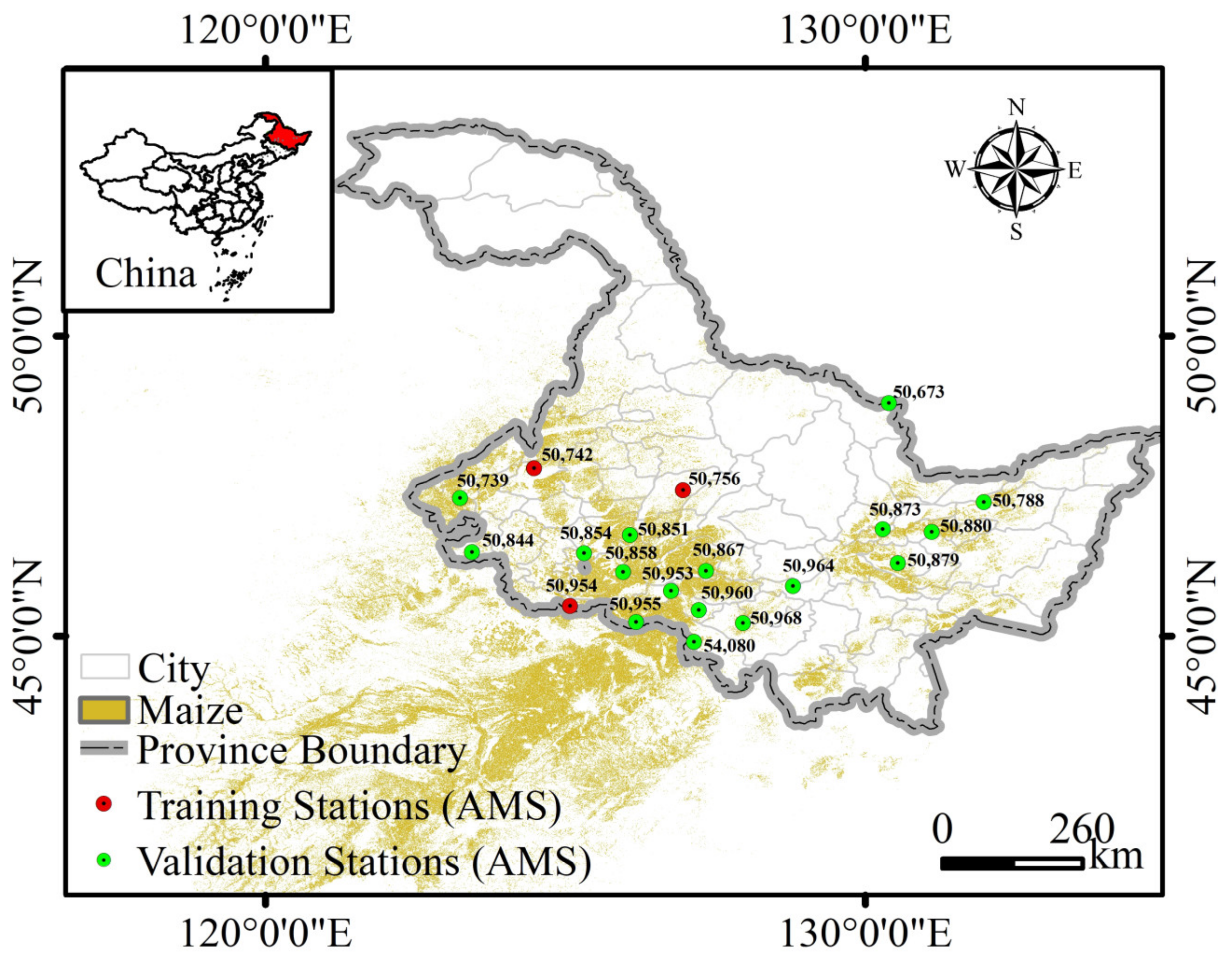
2.1. Study Area

China is the world’s second-largest maize producer and consumer, producing 23% of maize from only 9% of cultivated land and feeding approximately 22% of the global population [38]. The Northeast accounts for 31.51% of China’s maize planting area and contributes roughly 34.33% of maize production (http://www.stats.gov.cn/sj/ndsj/, accessed on 10 November 2023). As shown in Figure 1, our study focuses on Heilongjiang Province in northeastern China, with a maize area of 8.3 million ha, an important grain production base [39]. The predominant soil types are Chernozems, Meadow soil, and Black soil with abundant organic matter. The study area belongs to the cold-temperate continental semi-humid climate, with an average temperature above 17 °C in the crop-growing season, coupled with an average precipitation range of 400–650 mm. It is a rain-fed agricultural area without artificial irrigation, with maize typically sown around 118 days and harvested around 265 days. The main cropping pattern is maize and soybean rotation [40].

2.2. Dataset

2.2.1. Remote Sensing Data

This study utilized Sentinel-1 images as the primary dataset (Table 1). All images from 2017–2018 were used to detect annual maize phenology. They were obtained from the Google Earth Engine (GEE) collection “COPERNICUS/S1_GRD”. The observation pattern is the Interferometric Wide mode, including ascending and descending orbits, and provides dual polarization imagery with 10 m resolution. Sentinel-1 employs a 12-day repeat cycle for observing the Earth’s land surfaces [42] (Figure 2). Descending orbit data were utilized, as ascending orbit data were not available in the study area. The incidence angle of the images spanned from 30.0° to 45.0°. The speckle noise was reduced by a refined Lee speckle filter with a window size of 7 × 7 [43]. Then, the Shuttle Radar Topography Mission was used to correct SAR geometric distortions. Co-polarized (VV) and cross-polarized (VH) bands were converted to raw (i.e., no dB scaling applied) backscatter coefficient σ (i.e., Sigma naught), which is a measure of the reflective strength of a radar target per unit area. Although sigma 0 dB can be useful for visualizing the data and improving the contrast between different features, it is not recommended for phenological studies due to the introduction of distortions and artifacts in the data. Then, we calculated the CR to analyze its relationship with maize phenology.
This study acquired the top-of-atmosphere (TOA) reflectance of Sentinel-2 from the GEE collection “COPERNICUS/SENTINEL 2” because the Sentinel-2 surface reflectance (SR) products have only been available since 2018 in the study area (Table 1). The quantity of available TOA reflectance images is much greater than that of SR, facilitating the construction of time series spectral indices. The Sensor Invariant Atmospheric Correction method was used for atmospheric correction [44]. Sentinel-2A and -2B observe earth’s land surfaces with a 5-day repeat cycle and a 10–60 m spatial resolution [42] (Figure 2). The Normalized Difference Vegetation Index (NDVI) and Enhanced Vegetation Index (EVI) were calculated using Band 8 (785–900 nm), Band 4 (650–680 nm), and Band 2 (458–423 nm). Then, this study extracted the various phenological stages from Sentinel-2’s EVI time series based on harmonic fitting and compared them with the results of the CR time series. Additionally, maize layers were collected to mask maize planting areas. It is a new 10 m crop-type map in Northeast China from 2017 to 2018 with an overall accuracy of 91% [42].

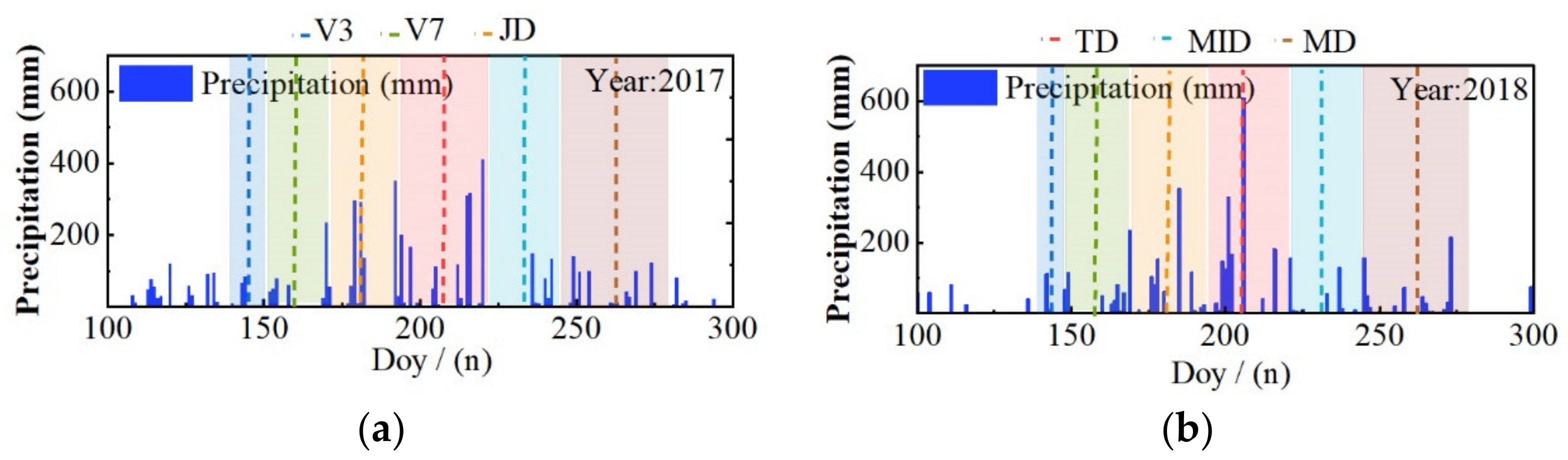
2.2.2. Ground Observation Data

This study collected ground observation data to validate our results. They were obtained from the Agricultural Meteorological Stations (AMSs) of the Chinese Meteorological Administration (CMA) (https://data.cma.cn/, accessed on 10 November 2023). A phenological stage is deemed to occur when more than 50% of maize fields have reached a particular stage. The recorded phenological stages include the emergence date (ED), V3, V7, JD, TD, MID, and MD of maize (Table 2). These phenological data were collected by well-trained agricultural technicians, and quality was controlled by the Department of China Agricultural Weather Monitoring System [45].
Additionally, this study acquired the daily precipitation, average wind speed, and maximum wind speed (MWS) (Daily Meteorological Data, DMD) to analyze their effect on Sentinel-1 features. Moreover, GDDs are calculated using the China meteorological forcing dataset (1979–2018) [46] (Table 1). It represents the effective temperature accumulated to complete a reproductive stage under the influence of environmental factors, which are utilized to analyze the results’ spatial distribution.
Table 1. Date used in this study.
DataApplicationSource
Maize layerMaize mask layer[42]
Sentinel-1Extraction of VH, VV, and CRGEE
Sentinel-2Extraction of EVI and NDVI time seriesGEE
AMSsValidation of maize phenology resultsCMA
DMDAuxiliary analysisCMA
GDDAuxiliary analysis[47]
Table 2. The phenological stages of maize.
Phenological StageDescription
Emergence dateThe date when the plant’s first true leaf unfolds and the seedlings are exposed 2 cm to 3 cm above the surface.
Three-leaves dateThe date when the third leaf is fully expanded.
Seven-leaves dateThe date when the seventh leaf is fully expanded.
Jointing dateThe date when the internodes at the base of the plant stem elongate.
Tassel dateThe date when the main tassel of the plant emerges 3–5 cm above the top leaf.
Milky dateThe date when the kernel color in the middle of the plant ear begins to show the inherent color of the variety, and the endosperm turns milky to mushy.
Maturity dateThe date when the dry weight of maize grains first reaches the maximum.
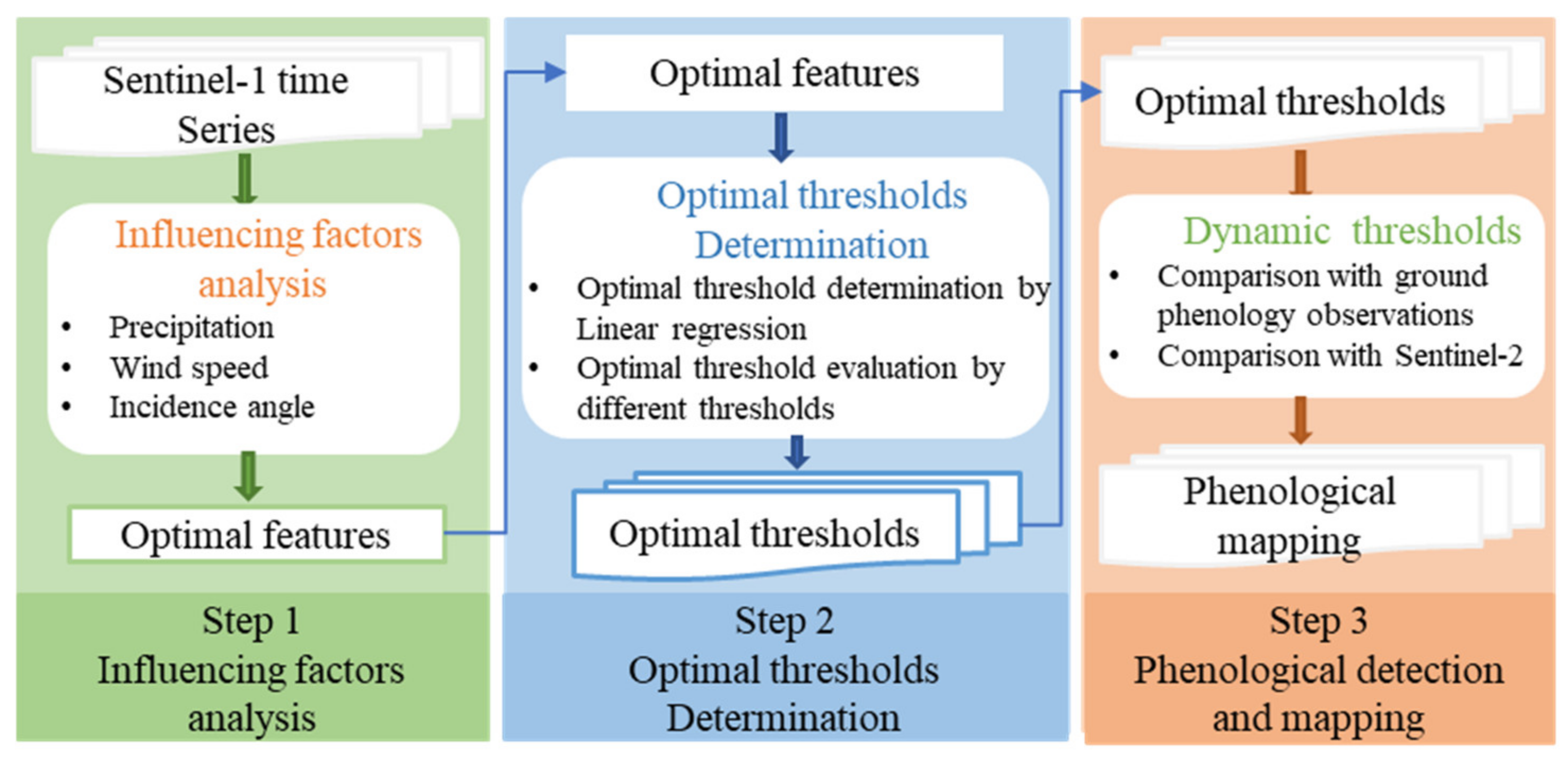
3. Methodology

An adaptive dynamic threshold method was developed to evaluate the ability of the Sentinel-1 time series to detect maize phenology (Figure 3). First, we used the correlation coefficient and standard deviation (SD) to analyze the effects of incidence angle, precipitation, and wind speed on Sentinel-1, aiming to screen the optimal feature. The optimal threshold for different phenological stages were determined by linear regression, and their effectiveness was evaluated by employing various threshold settings. Second, we applied the optimal threshold to detect crop phenology on a regional scale. Moreover, we evaluated the accuracy of the detection results with ground observation data and compared them with the results of Sentinel-2, thereby verifying the efficacy of the adaptive dynamic thresholds. Finally, the phenological detection results were mapped at a regional scale, and their rationality was analyzed using GDDs.

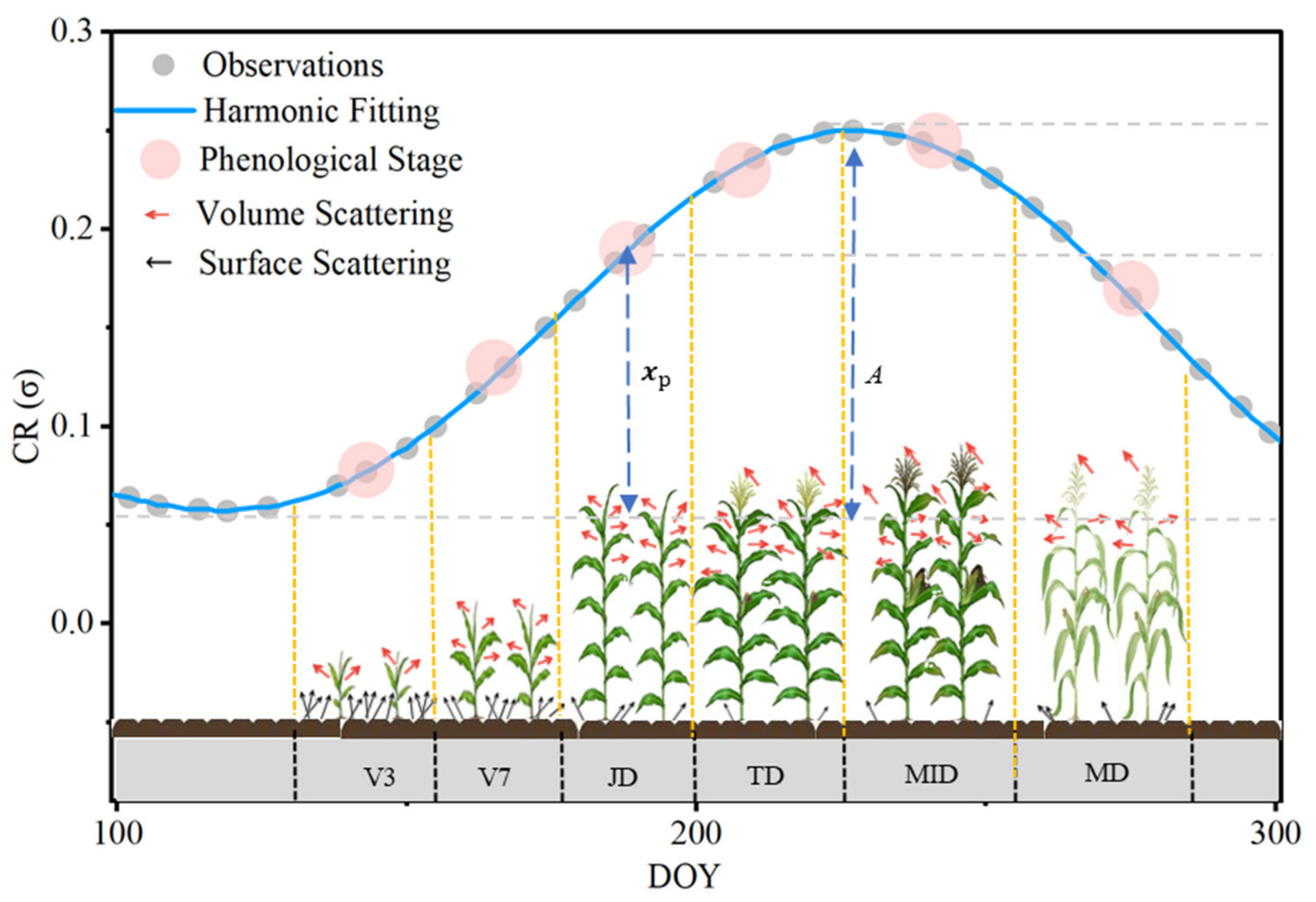
3.1. Optimal Sentinel-1 Feature Analysis

Objectively determining the crop phenological stages from Sentinel-1 satellite observations is challenging, particularly during the crop-growing period, owing to the complex backscattering mechanism. From V3 to V7, the Sentinel-1 backscatter is dominated by the surface scattering of soil due to small maize plantings, resulting in the majority of the soil being visible [27,28] (Figure 4). As the crop grows and canopy cover increases, surface scattering from the soil decreases, while volume scattering of the canopy gradually increases from JD, reaching its peak during the TD and MID. Even as the canopy withers by MD, exposing some soil, volume scattering from the canopy remains dominant.
Precipitation, wind speed, and incidence angle are the main factors driving the variations in SAR features, affecting total ground biomass, plant geometry, and vegetation water content [47,48]. Consequently, we calculated the Pearson correlation coefficients between the precipitation, wind speed, incidence angle, and Sentinel-1 features at different phenological stages to determine the optimal feature. Moreover, we compared the changes in Sentinel-1 features with the phenological development at various incident angles. The more stable Sentinel-1 time series is conducive to phenological detection. Therefore, the SD of the Sentinel-1 time series was calculated to assess the stability of different features.

3.2. Adaptive Dynamic Threshold

In the original dynamic threshold method (Equations (1) and (2)),   M is the maximum value of the feature. m l and m r are the minimum values of the feature at the beginning and end of the growing season, respectively. m is the average of the m l and m r . A is the amplitude, which is the difference between M and m . P indicates the date of the detected phenological stage. In general, the amplitude threshold ( T ) is empirically determined for detecting the beginning and end of the growing season, such as 20%, 50%, etc. [49]. However, this threshold is inevitably influenced by subjective factors. Moreover, the thresholds for detecting the phenological stages exhibit significant variations across different features, particularly between optical indices and SAR features.
A = M m
P = m + A T
Therefore, this study used a linear regression approach to determine optimal thresholds (CRs) for detecting various phenological stages. CR has been widely used in agricultural studies due to its lack of influence from clouds and rain, along with its fine spatial resolution. Furthermore, CR is sensitive to vegetation stems and canopy structures. Ridges and ditches at the edges of corn fields may be mixed into corn pixels. Therefore, morphological processing was applied to erode the maize planting area, eliminating non-maize pixels. This study used the mean value from mid-April to early May as the minimum ( M i n g ) value of CR during the growing season. As this period is bare soil, the CR value is the lowest, which avoids the failure to detect CRs in other phenological stages. The amplitude ( A g ) is the difference between the maximum value ( M a x g ) and M i n g . The A g and the real CR (extracted from Sentinel-1 according to the recorded phenological data) were independent variables. These variables values are extracted from the buffer zone within 5 km of each AMS because the study [50] demonstrated that 5 km is an acceptable spatial scale for remote sensing phenology and ground observation. They are under similar climate and soil conditions. And as shown in Equation (3), the optimal threshold for each phenological period was obtained by linear regression. Since the CR calculated based on the threshold determines the accuracy of phenological detection, the performance of the optimal threshold was evaluated by calculating the RMSE between the threshold (with a step of 0.1) and the actual CR at each phenological stage. This was compared with the estimated CR by the adaptive dynamic threshold method. A smaller RMSE between the optimal threshold estimated CR and the actual CR at the phenological stage indicates the effectiveness of the adaptive dynamic threshold method. There were only three randomly selected AMSs to determine the optimal threshold for dynamic phenological detection at the provincial scale. This approach not only avoids numerous field surveys but also allows for the quick detection of region-scale crop phenology.
T = i = 1 n x p i = 1 n A g
where T represents the optimal threshold for each phenological stage, such as V3, V7, JD, TD, MID, and MD of maize; A g   is the amplitude of the CR; x P is the difference between the real CR and M i n g ; i is a pixel within 5 km of the AMS. n   is the number of pixels within 5 km of the AMS.
Equation (3) is substituted into Equation (2) to avoid the threshold exceeding the CR maximum, which may result in the failure to detect the corresponding CR value and obtain the phenological stages. M i n g was used instead of m . Thus, the adaptive dynamic threshold (Equation (4)) for detecting phenological stages P I is derived as follows:
P I = M i n g + A g × T
In addition, the harmonic function was utilized to fit the CR time series at a daily resolution before conducting crop phenology detection [51]. Then, the phenology was detected using the adaptive dynamic threshold. It should be noted that to obtain a better detection result, the fitting function will also change according to the feature time series.

3.3. Accuracy Assessment

The adaptive dynamic threshold was used to map spring maize phenology for two years (2017–2018) in Heilongjiang Province. To assess the accuracy of the map, ground phenology observation data were compared with the results of Sentinel-2 extracted by the original dynamic threshold method. Specifically, the dates for V3, V7, and JD were determined when the EVI first crossed 10%, 15%, and 50% of the segment EVI amplitude, and TD is the maximum EVI amplitude. MID and MD are the dates when the EVI last crossed 90% and 50% of the segment EVI amplitude. These thresholds refer to Niu et al. [22] and MCD12Q2.
Ground phenological observations from all stations were used for validation, except for three randomly selected observations in 2017, which were used to determine the optimal threshold (Figure 1). Moreover, to assess the inter-annual applicability of the threshold, validation was performed not only for the detection results of 2017 but also those of 2018. The root mean square error (RMSE, Equation (5)) and coefficient of determination (R2, Equation (6)) were calculated to assess the results. x t   is the ground phenology observation data recorded by the AMSs, x p is the detection results, and m is the amount of ground phenology observation data. j is a ground phenology observation. x ¯ is the recorded average observation data. We calculated the RMSE between the detection results and ground phenology observation data within 5 km because it is less affected by the spatial scale between ground observations and satellite data [50,52].
RMSE = j = 1 m x t x p 2 n
R 2 = j = 1 m x t x ¯ 2 j = 1 m x p x ¯ 2

4. Results and Discussion

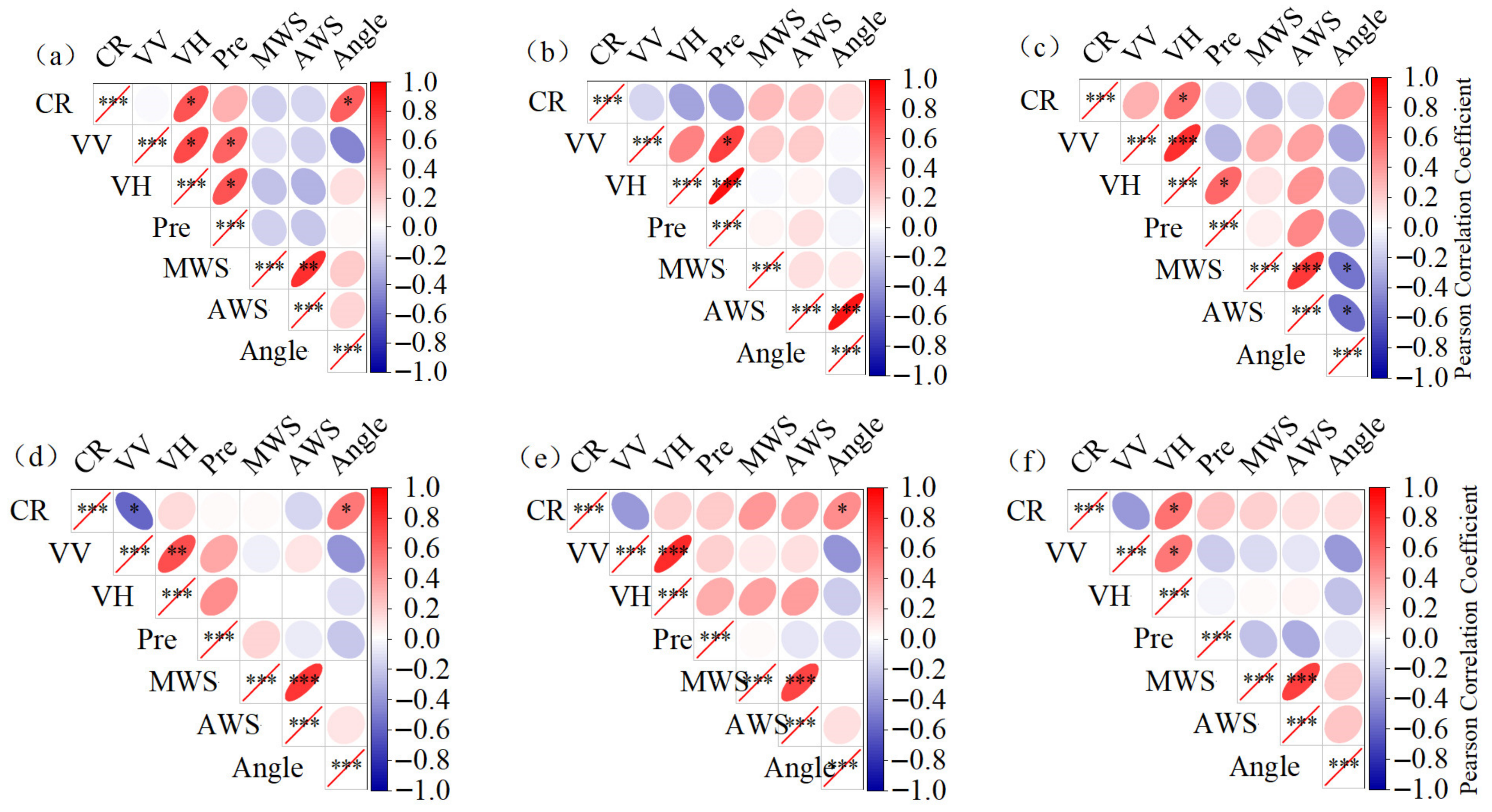
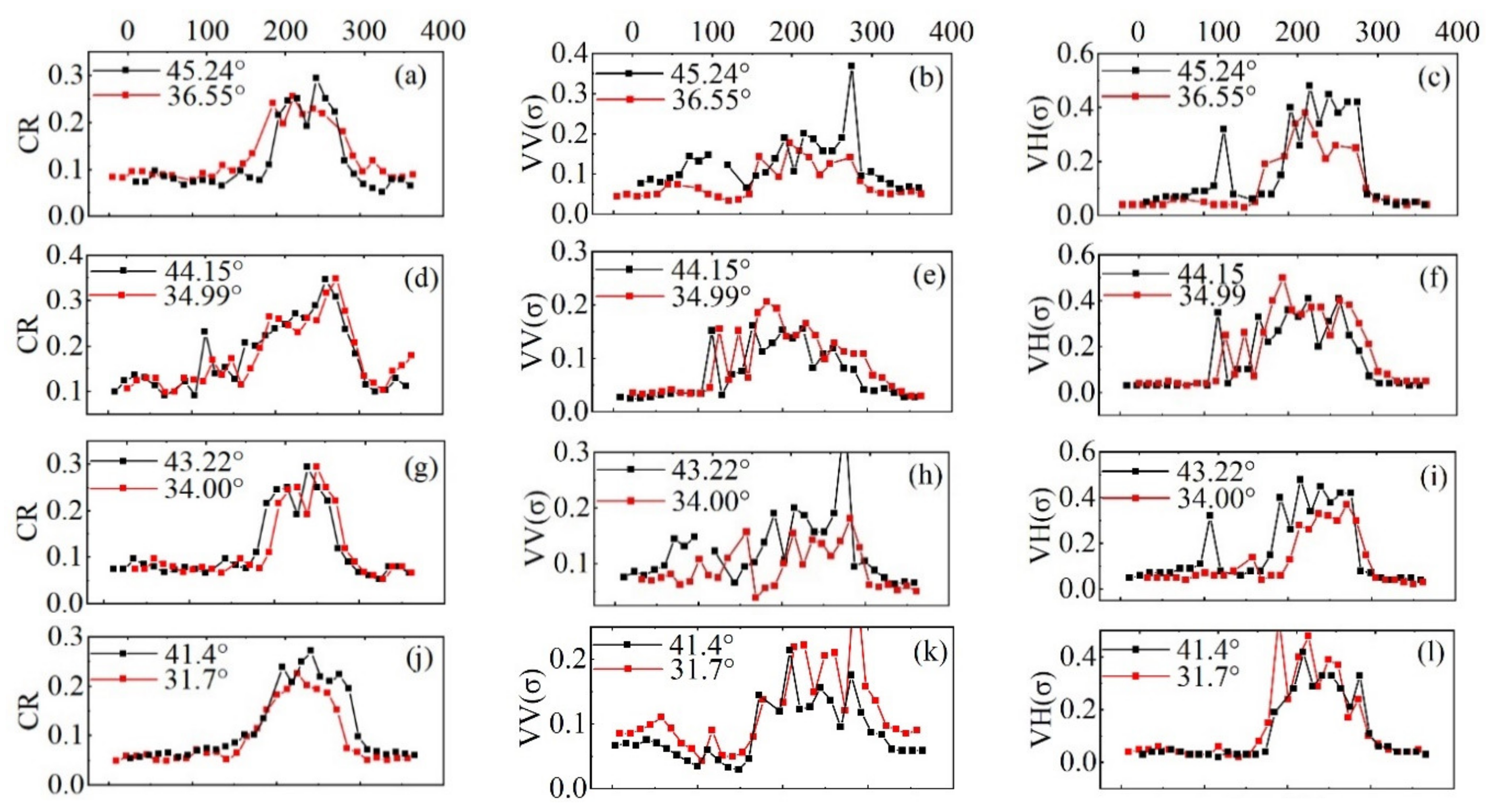
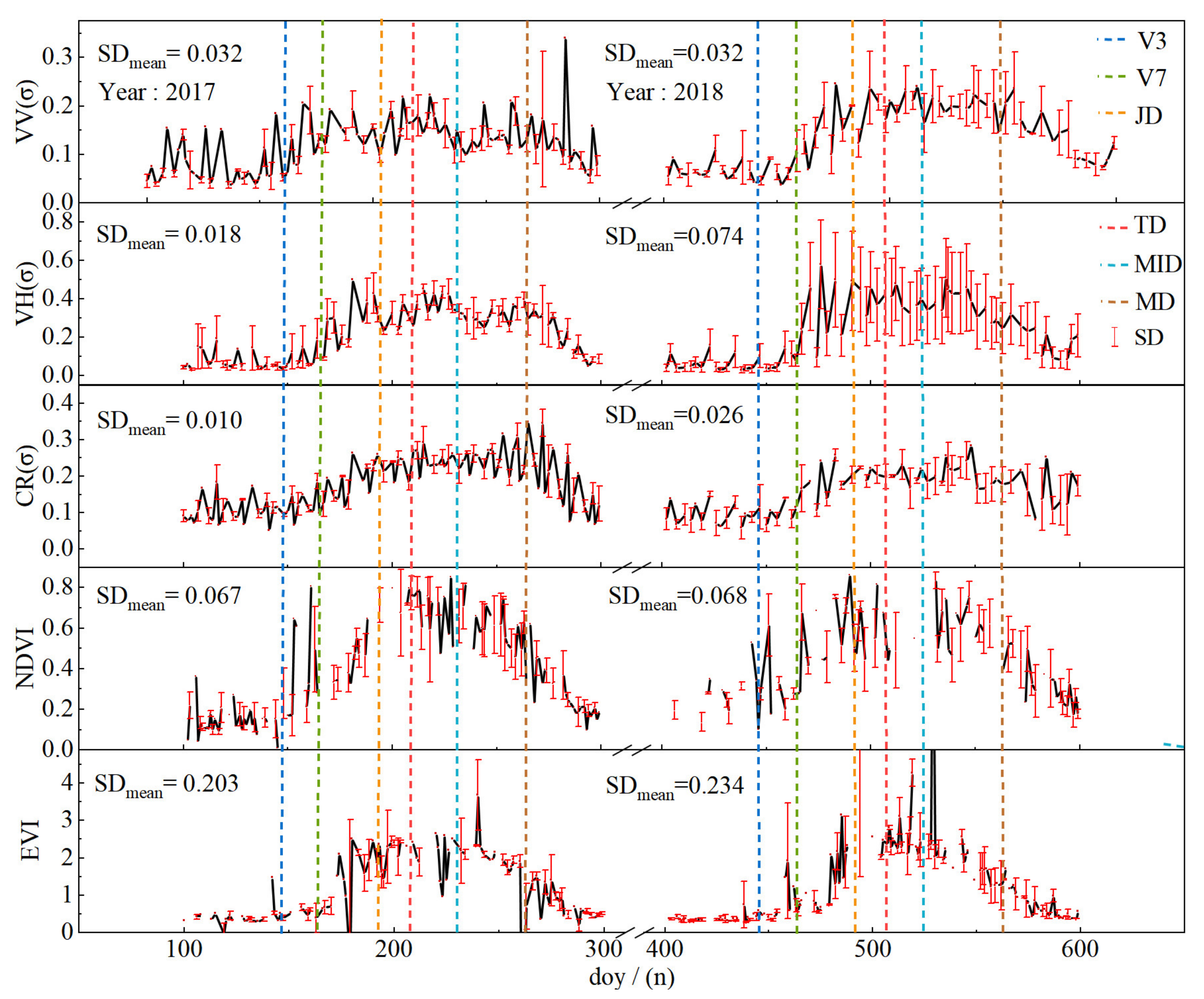
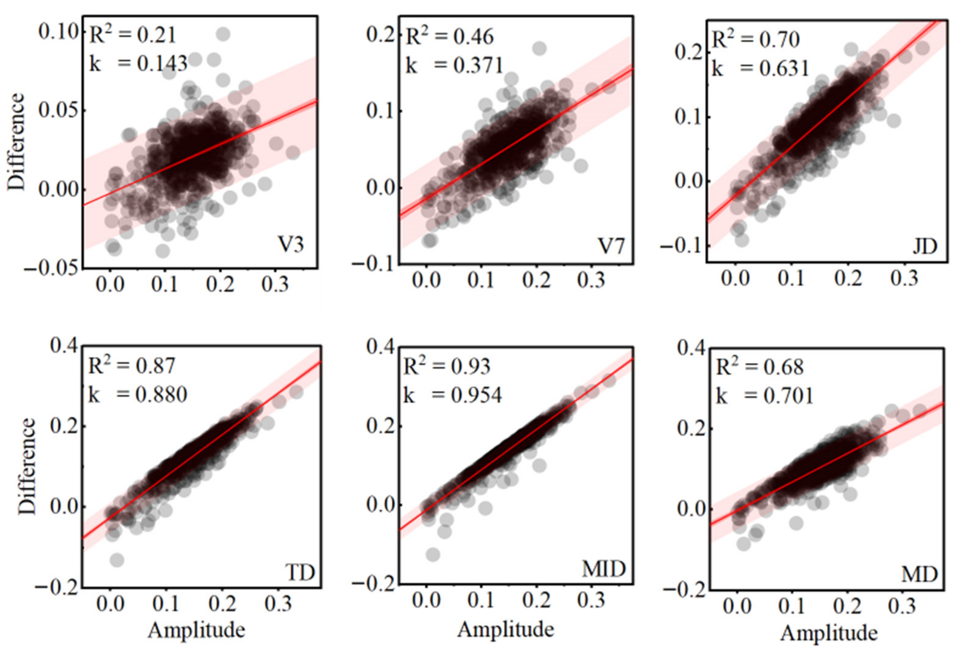
4.1. Influencing Factor Analysis of Sentinel-1 Features

The effects of incidence angle, precipitation, and wind speed on Sentinel-1 features were analyzed using statistical methods and a backscatter mechanism to determine the optimal features for phenology detection. In the VH, the contribution of multivolume scattering from canopy structures is more important [53,54]. Conversely, in the VV, direct surface scattering from the soil generally dominates [55]. Due to the maize’s vertical structure, VV attenuation is higher than VH. Consequently, VH is larger than VV, leading to a gradual increase in CR during crop growth. The CR at low incidence angles (30.66°, 31.70°, 34.00°, 34.99°) is lower than that at high incidence angles (40.81°, 41.40°, 43.22°, 44.15°) (Figure 5d,g,j,m). Notably, there is no significant difference between the incident angles of 36.55° and 45.24° (Figure 5a). This observation is consistent with previous research, indicating that higher incidence angles (>35°) lead to an increase in the path length through vegetation, thus maximizing the contribution of vegetation scattering [27,56,57]. Consequently, a higher incidence angle of CR is more sensitive to vegetation canopy and fresh biomass, benefiting vegetation phenology detection. In contrast to CR, VV, and VH displayed irregular trends as the incidence angle transitioned from low (<35°) to high (>35°). In addition, Schlund and Erasmi [34] have confirmed the effectiveness of normalizing observations collected from multiple view angles for CR.
Moreover, their influence was analyzed by calculating the correlation between precipitation, wind speed and Sentinel-1 features at various phenological stages. There was no significant correlation between wind speed and Sentinel-1 features. As shown in Figure 6, the influence of precipitation on Sentinel-1 features is VH > VV > CR. The influence of precipitation on Sentinel-1 features during the maize’s nutritional growth phase was more pronounced compared to the reproductive growth phase. For instance, precipitation displays a significant influence on VH in the V3 (r = 0.69, p = 0.05), V7 (r = 0.94, p = 0.001), and JD (r = 0.59, p = 0.01), while no significant effect is observed in the TD, MID, and MD. This variation can be attributed to the dynamic interplay between vegetation and soil contributions, which depends on factors such as crop development stages, soil moisture, soil roughness, and crop conditions [54]. For instance, the introduction of anisotropy into soil roughness by agricultural sowing rows could be observed when the soil is bare or sparsely covered by vegetation. Numerous studies [58,59,60] have documented the effect of row orientation on Sentinel-1 features. Over time, wind and precipitation tend to flatten the surface, reducing anisotropy [60]. During V3–V7, the influence of the precipitation on VH and VV increases significantly due to the sparse maize canopy. Subsequently, this effect decreases as the canopy density increases from V7 to JD. However, precipitation has no significant effect on CR from V3 to MD (Figure 6), proving that CR mitigates the influence of precipitation and soil water content, which is consistent with existing studies [14,47,61]. At the same time, studies have indicated that when the LAI ranges between 1.0 and 3.0, the SAR response is predominantly influenced by vegetation and least affected by soil moisture conditions [62,63].
The stability of the Sentinel-1 features was assessed by calculating the SD of the features time series. VH, VV, and CR were extracted from Sentinel-1. NDVI and EVI were extracted from Sentinel-2. Figure 7 illustrates the average trends of the time series by calculating the mean values of the different site features for each day. Given the differences in environmental and human management practices, SD was used to reflect the stability of VV, VH, and CR on the regional scale. Specifically, the study area included 20 phenological observation sites, from which VH, VV, CR, NDVI, and EVI values were extracted from the V3 to the MD. Their daily SDs were then calculated. Compared with VH and VV, the SD of CR is the smallest, even though the value range of CR is not the smallest. This indicated that CR is the least affected by the environment and variations in agricultural practice [34]. Studies have also demonstrated strong agreement between CR time series for crops such as maize, barley, and winter wheat and destructive measurements of the green area index and fresh biomass measurements [34,47]. And the CR time series is closely similar to that of NDVI (r = 0.70) and EVI (r = 0.71). Moreover, CR is less affected by precipitation, soil water content, and surface roughness than VH and VV [14,47]. Consequently, CR was chosen as the optimal feature to detect phenology.

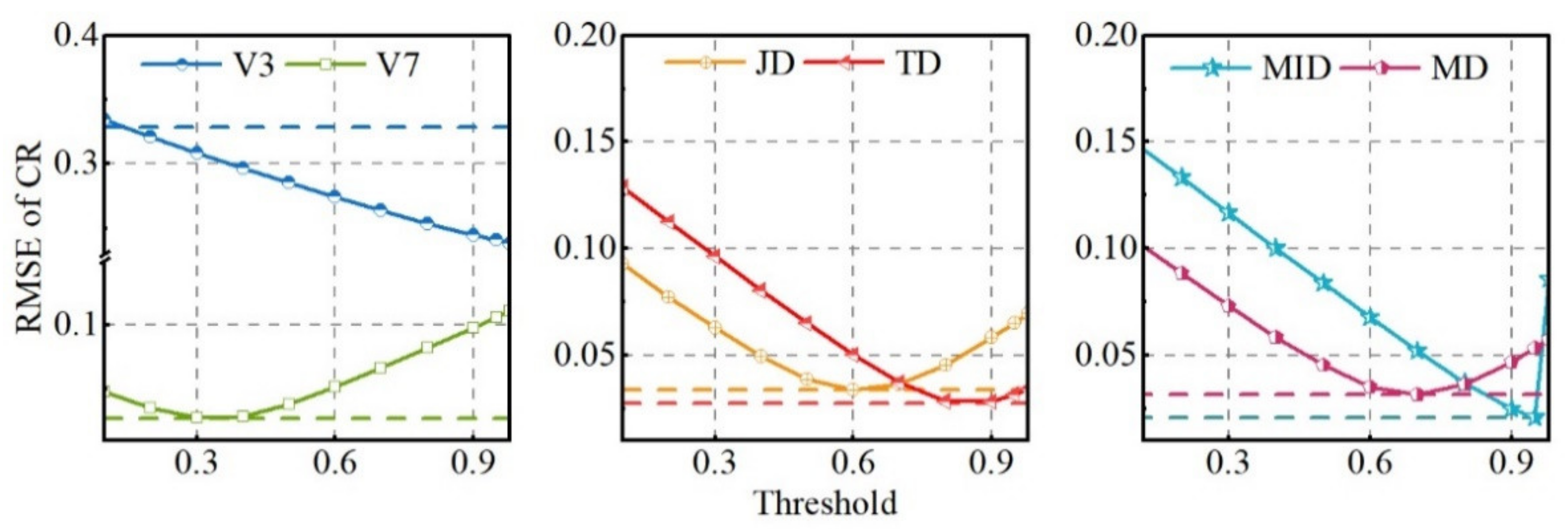
4.2. Analysis of Optimal Threshold

Under the selected optimal Sentinel-1 feature (CR), linear regression fitting was conducted between x P and A g to determine the optimal threshold for detecting various phenological stages (Figure 8). The R 2 of the optimal threshold ranged from 0.21 to 0.46 for V3 to V7 and from 0.68 to 0.93 for MID to MD. These R 2 values of the optimal thresholds are closely related to the different phenological stages. As shown in Figure 8, spatial variation in CR is mainly reflected in different phenological stages. The scatter of CR from V3 to MD transitions from a dispersed pattern to aggregated mode and back to dispersed mode, respectively. This variance is mainly due to the greater contribution of soil moisture and surface roughness compared to the maize canopy in V3 and V7 [47,64], resulting in the high spatial heterogeneity of CR and lower R 2 of these two phenological stages. At the JD-MID stage, with the canopy gradually covering the soil, VH and VV are mainly influenced by volume scattering, leading to the spatial distribution of CR becoming more aggregated. The R 2 of the optimal threshold reaches a maximum at the MID ( R 2 = 0 .93). Subsequently, as the maize matures with canopy water loss and leaf senescence, the dominance of maize volume scattering gradually decreases, and the spatial variability of CR increases. Overall, the CR time series could reflect the growth cycle of maize. However, the ability to detect different phenological stages may be significantly different. For example, the difference between TD and MID in CR is smaller than that in other phenological stages, resulting in serious confusion between them. Previous studies have shown that SAR signals are saturated at the maximum fresh biomass of maize [55].
In addition, to evaluate the performance of the optimal threshold determined by linear regression, we calculated the RMSE between the CR of dynamic threshold with a step of 0.1 and the actual CR (Figure 9). This evaluation focused on the threshold itself rather than comparing the detected phenological date with the date recorded by the AMSs. As depicted in Figure 9, except for V3, the RMSE decreases and then increases with changes in the threshold for all the phenological stages. Moreover, the RMSE of the optimal threshold determined by the dynamic threshold consistently remains the minimum. The results show the effectiveness of the adaptive dynamic threshold method in extracting the optimal threshold for detecting different crop phenological stages. For V3, the challenge might arise from the small size of the crop, leading to Sentinel-1’s 10 × 10 grid predominantly reflecting the soil background. This scenario complicates the determination of the optimal threshold for phenological detection.

4.3. Validation of Ground Phenology Observation Data

This study designed an adaptive dynamic threshold approach to detect maize phenology using the Sentinel-1 time series. The results indicated that the R2 in two years was 0.813 and 0.804, respectively, and both were significant at the 0.001 level (Figure 10). As shown in Figure 11, the precision of maize phenology from high to low was MD > JD > MID > V3 > TD > V7 in 2017. And the precision of maize phenology from high to low was MID > MD > JD > V3 > TD > V7 in 2018. The RMSEs of JD, MID, and MD are significantly lower than those for V3, V7, and TD in two years. This indicated that the Sentinel-1 time series is better at detecting JD, MID, and MD compared to V3, V7, and TD. It is worth noting that the optimal threshold derived from the 2017 data was used for estimating maize phenology in both 2017 and 2018, based on data from only three AMSs. This consistency implies the stability of optimal thresholds across different years. When ground phenological observation data for a particular year are unavailable, historical ground phenological observation data can be utilized to quickly obtain crop phenology at the regional scale. However, the dates of V3 and V7 detected by the adaptive dynamic threshold method are earlier than those recorded by ground phenology observation data. This discrepancy could be attributed to the complex interaction of crop canopy, soil background, and precipitation. Because the CR is sensitive to the three-dimensional structure of the soil canopy, canopy backscattering is mainly influenced by the angle and size of the leaves, water content, and wavelength of incidence [65,66]. During the nutritional growth phase of maize, the smaller size (plant height is about 20 cm) of the plant’s stems and leaves at V3 results in backscattering primarily reflecting the soil background. Precipitation events further influence backscatter coefficients, leading to the earlier detection of V3 (Figure 12). At V7, the multiple scattering effects between soil and canopy structure contribute significantly to the total backscatter. Given that maize is a broad-leaved crop, the size and angle of the leaves and the spacing of the plant rows affect multiple scattering effects [67], resulting in greater error variation. In addition, at TD, the maize plants have fully developed leaves, dry matter accumulation is the highest, maize pollination begins, and the CR maintains a slight increase approaching saturation [63]. Therefore, the detection date of TD tends to be significantly later than the date recorded by ground phenological observation data.

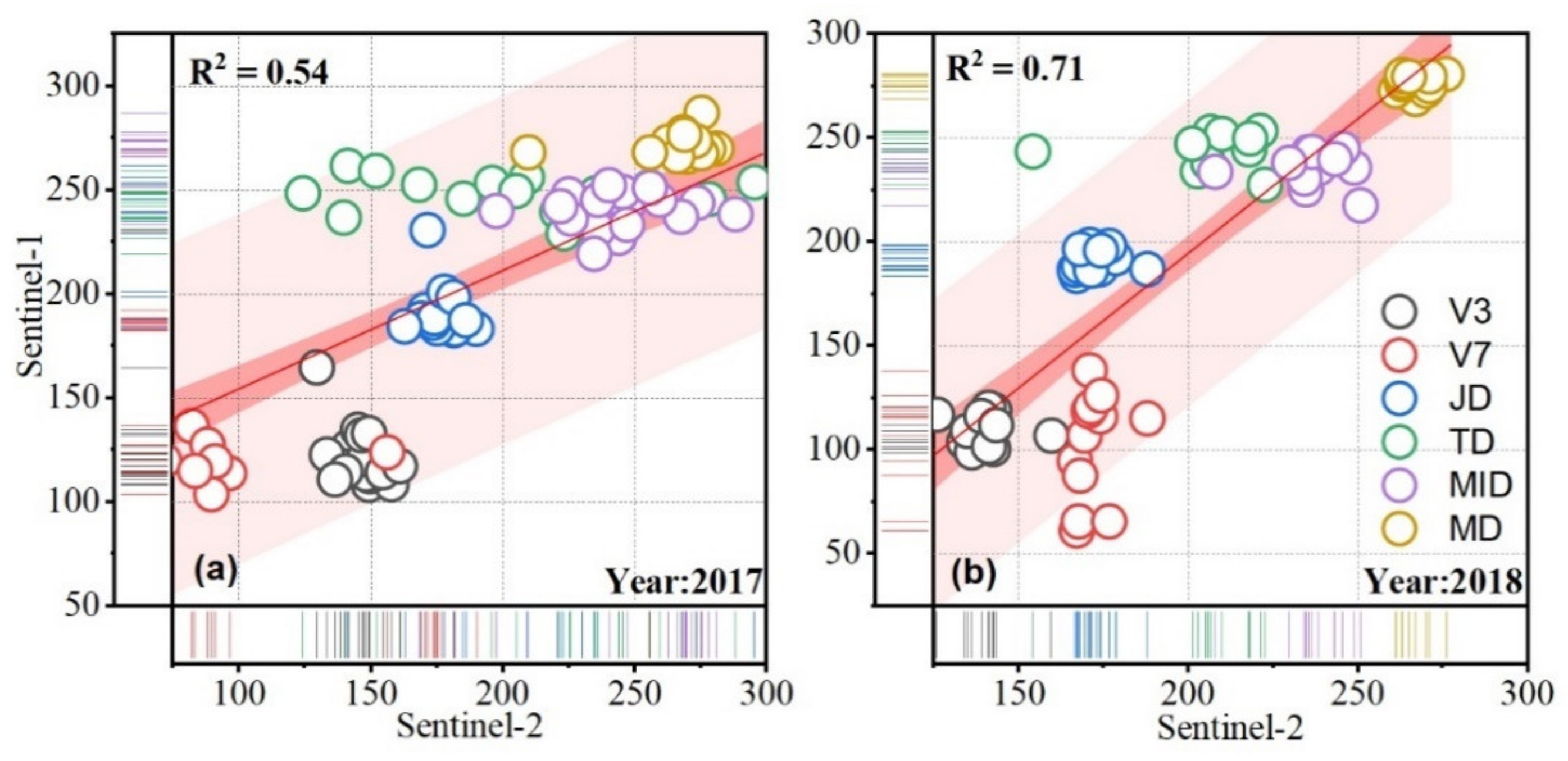
4.4. Comparison of Sentinel-1 and Sentinel-2 Phenology Observations

This study detected different phenological stages using the EVI time series and compared them with the results of CR time series (Table 3). Notably, although Sentinel-2’s maximum image count is larger than that of Sentinel-1’s, the RMSE indicated that Sentinel-1 can stably detect JD, TD, and MID in 2017 and 2018. Specifically, the average RMSE for JD, MID, and MD decreased by 4.14%, 35.28%, and 26.48%, respectively, when compared to Sentinel-2 phenology observations. Therefore, the quantity of images did not significantly impact the Sentinel-1’s detection results. Sentinel-2 is the most stable in detecting V3 and JD, but for other phenological stages, the RMSEs varied significantly in different years. For instance, the RMSEs for V7 and TD in 2017 were significantly higher than those in 2018. This could be attributed to image acquisition coinciding with a significant rainfall event in 2017, resulting in a higher overall RMSE for each phenological stage. Overall, Sentinel-1 effectively detects JD, MID, and MD under continuous clouds and rainfall. In addition, compared to Sentinel-2 phenology observations, our results underestimated the V3, V7, and MID and overestimated the JD and TD for maize (Figure 13b). This indicated that the CR time series and EVI time series for broad-leaved maize did not completely match (Figure 7). For example, in the nutritional growth phase of maize, V3, V7, JD, and TD correspond to the dates when EVI first crossed 10%, 15%, and 50% and reaches its maximum amplitude, respectively, which is faster than the phenology detected by the CR. The same is true for the reproductive growth phase. This inconsistency is consistent with previous studies [14,27], which have highlighted differences between NDVI and CR time series for maize in various regions. The reason could be the different response principles of two indices to vegetation. EVI responds to changes in leaf area and chlorophyll content. CR is sensitive to changes in soil cover and structural plant development. Consequently, their changes did not completely match. Veloso et al. [34] have shown that CR exhibits a higher correlation with fresh biomass compared to photosynthetic activity. For example, as crops mature, EVI decreases due to the leaf yellowing and drying, which reduces the chlorophyll content and increases lutein content [68,69]. In contrast, CR responds to standing, yellowing crop structures (or maize stubble) [14,34], leading to differences in the EVI and CR time series.

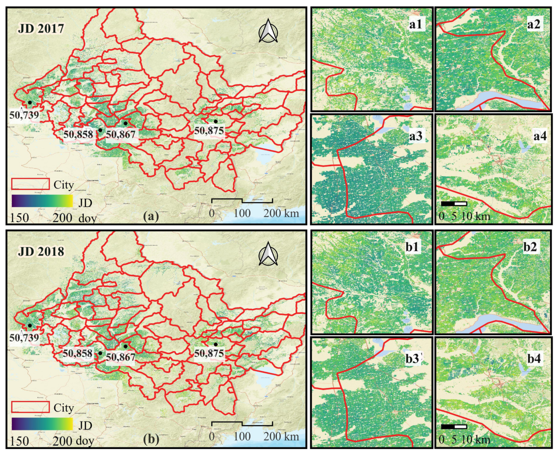
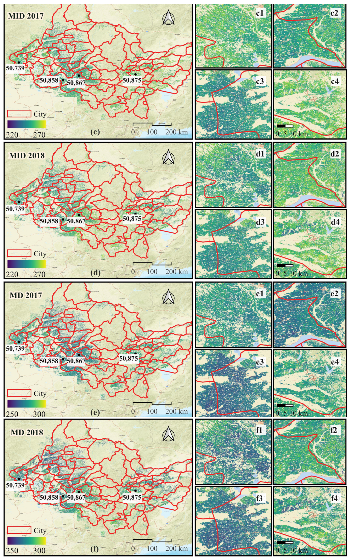
4.5. Mapping Maize Phenology in Heilongjiang Province

We compared the abilities of adaptive dynamic thresholds in mapping spring maize phenology for the years 2017 and 2018 in Heilongjiang Province. Figure 14 illustrates the estimations for JD, MID, and MD. However, due to the large errors in V3, V7, and TD, their spatial distribution has no reference. Overall, consistent spatial variation in phenological development was observed in 2017 and 2018, with earlier development occurring in the southern regions compared to the northern regions. This spatial variation can primarily be attributed to GDDs, a key factor affecting crop phenological development [70,71]. In this study area, the number of GDDs in the south is always higher than that in the north. Meanwhile, we calculated the GDDs for the years 2017 and 2018, revealing coherent spatial variations in the accumulated temperature (Figure 15). Specifically, although the accumulated temperature in 2018 (GDDs = 3186 °C) was generally higher than that in 2017 (GDDs = 3120 °C), their spatial distribution remained consistent. This consistency accounts for the spatial similarity in observed phenological patterns. The region with lower GDDs in the north may benefit from employing early-maturing crop varieties with a shorter growth period to increase grain yield. In addition, natural disasters and field management may exacerbate phenological differences between adjacent years within the same area. For example, at site 50,858, the phenological development in 2018 is earlier than that in 2017.

4.6. Limitations and Outlook

Phenological monitoring using the adaptive dynamic threshold method, based on data from the GEE, offers a practical solution for monitoring phenology with limited sample sizes. In agricultural applications, this approach requires collecting regional ground phenology observation data (3–5 samples). Subsequently, the amplitude, minimum value, and CR of the phenological observation date are extracted to calculate the optimal threshold. Finally, phenology mapping is performed based on the optimal threshold. (https://code.earthengine.google.com/cb00adc3488a10f7de3da2a395b87fc1 accessed on 10 November 2023). And the approach only needs to change the threshold of different regions to realize phenology mapping. In addition, the approach utilizes SAR time series, which are unaffected by clouds or precipitation, thereby providing reliable phenology information.
However, this approach still has some limitations for application to larger areas, different crop types, and more phenological stages. First, the spatial heterogeneity of crop seeding density, soil background, and precipitation [28,72] in a larger area could affect the backscattering intensity, increasing the phenological detection uncertainty. Second, limited by the availability of crop samples, this method has not yet been applied to crops other than maize. If the monitored crop structure is very different from maize, such as soybean and rice, the accuracy of the method could be decreased because the difference in vegetation structure reflects the difference in backscattered signals. Third, this approach, which utilizes a single feature as input, is beneficial for quickly detecting crop phenology at the regional scale. However, one feature can only provide limited information; it cannot characterize the actual and complex physiological changes of crops. Finally, it should be noted that when the pixels have a lower spatial resolution, the calculated thresholds should be interpreted cautiously because there could be more mixed pixels [25]. In the future, to improve phenological detection accuracy in larger areas, regional thresholds should be taken to mitigate the effects of anthropogenic management and the variety of geographical environments. Additionally, studies have explored the potential of monitoring the entire crop growth stage using multisource remote sensing data [14,52], which could improve the accuracy of phenological monitoring.

5. Conclusions

This study developed an adaptive dynamic threshold method that autonomously determines the optimal threshold for crop and environmental classification, eliminating the requirement for human intervention. Moreover, it evaluates not only SAR data’s capability of detecting TD and MID but also assesses SAR’s potential for detecting V3, V7, TD, and MD. We first analyzed the Sentinel-1 features to select optimal features for time series fitting. The results revealed that the CR is least affected by incident angle, precipitation, and wind speed, making it a robust indicator for capturing phenological development accurately while minimizing noise. Then, we employed linear regression to determine the optimal threshold, thereby avoiding the subjectivity of custom thresholds. This is not possible with traditional dynamic threshold methods. This study demonstrated that the ability of the Sentinel-1 time series to detect JD, MID, and MD is greater than that of V3, V7, and TD. Moreover, the adaptive dynamic threshold was built to detect crop phenology at a regional scale, improving detection accuracy compared to Sentinel-2 phenology observations. The average RMSEs of JD, MID, and MD decreased by 4.14%, 35.28%, and 26.48%, respectively. Furthermore, we analyzed the spatial distribution of JD, MID, and MD of maize in 2017 and 2018, revealing a correlation between phenological patterns and GDDs. The crop phenology was delayed with increasing latitude. It should be noted that the adaptive dynamic threshold is generically applicable to different broad-leaved crops. The overall strength of backscattering increased with maize growth, and similar backscattering is observed in other broad-leaved stalk crops (e.g., sorghum) [73,74].

Author Contributions

Conceptualization, Y.M.; methodology, Y.M.; software, Y.M.; validation, Y.M.; formal analysis, Y.M., H.G. and J.L.; investigation, C.H., G.J. and Y.S.; resources, Y.D. and Y.S.; data curation, Y.M. writing—original draft preparation, Y.M.; writing—review and editing, J.H. and H.G.; supervision, J.H., C.H., G.J. and Y.S.; project administration, C.H., G.J. and Y.S.; funding acquisition, C.H., G.J. and Y.S. All authors have read and agreed to the published version of the manuscript.

Funding

This research was funded by the National Nature Science Foundation of China Program (Grant No.: 42071380); the National Natural Science Foundation of China (Grant No.: 42271397); and the Open Fund of the Key Laboratory of Geography and National Conditions Monitoring of the Ministry of Natural Resources, China (2022NGCM05).

Data Availability Statement

The data that support the findings of this study were obtained from the Google Earth Engine (https://earthengine.google.com/, accessed on 10 November 2023) and the Chinese Meteorological Administration (CMA) (https://data.cma.cn/, accessed on 10 November 2023). They are available from the W.S. and Y.S., upon reasonable request.

Conflicts of Interest

Author Gongxin Jiang was employed by the company Hubei Ecological Environmental Protection Co., Ltd. The remaining authors declare that the research was conducted in the absence of any commercial or financial relationships that could be construed as a potential conflict of interest.

References

  1. Ranum, P.; Peña-Rosas, J.P.; Garcia-Casal, M.N. Global maize production, utilization, and consumption. Ann. N. Y. Acad. Sci. 2014, 1312, 105–112. [Google Scholar] [CrossRef]
  2. Luo, Q.; O’Leary, G.; Cleverly, J.; Eamus, D. Effectiveness of time of sowing and cultivar choice for managing climate change: Wheat crop phenology and water use efficiency. Int. J. Biometeorol. 2018, 62, 1049–1061. [Google Scholar] [CrossRef]
  3. Gao, F.; Anderson, M.C.; Zhang, X.Y.; Yang, Z.W.; Alfieri, J.G.; Kustas, W.P.; Mueller, R.; Johnson, D.M.; Prueger, J.H. Toward mapping crop progress at field scales through fusion of Landsat and MODIS imagery. Remote Sens. Environ. 2017, 188, 9–25. [Google Scholar] [CrossRef]
  4. Wang, C.; Han, J.; Shangguan, L.; Yang, G.; Kayesh, E.; Zhang, Y.; Leng, X.; Fang, J. Depiction of grapevine phenology by gene expression information and a test of its workability in guiding fertilization. Plant Mol. Biol. Rep. 2014, 32, 1070–1084. [Google Scholar] [CrossRef]
  5. Huang, J.; Gómez-Dans, J.L.; Huang, H.; Ma, H.; Wu, Q.; Lewis, P.E.; Liang, S.; Chen, Z.; Xue, J.-H.; Wu, Y. Assimilation of remote sensing into crop growth models: Current status and perspectives. Agric. For. Meteorol. 2019, 276, 107609. [Google Scholar] [CrossRef]
  6. Pulatov, B.; Linderson, M.-L.; Hall, K.; Jönsson, A.M. Modeling climate change impact on potato crop phenology, and risk of frost damage and heat stress in northern Europe. Agric. For. Meteorol. 2015, 214, 281–292. [Google Scholar] [CrossRef]
  7. Wang, X.; Huang, J.; Feng, Q.; Yin, D. Winter Wheat Yield Prediction at County Level and Uncertainty Analysis in Main Wheat-Producing Regions of China with Deep Learning Approaches. Remote Sens. 2020, 12, 1744. [Google Scholar] [CrossRef]
  8. Huang, J.; Ma, H.; Sedano, F.; Lewis, P.; Liang, S.; Wu, Q.; Su, W.; Zhang, X.; Zhu, D. Evaluation of regional estimates of winter wheat yield by assimilating three remotely sensed reflectance datasets into the coupled WOFOST–PROSAIL model. Eur. J. Agron. 2019, 102, 1–13. [Google Scholar] [CrossRef]
  9. Badeck, F.W.; Bondeau, A.; Böttcher, K.; Doktor, D.; Lucht, W.; Schaber, J.; Sitch, S. Responses of spring phenology to climate change. New Phytol. 2004, 162, 295–309. [Google Scholar] [CrossRef]
  10. van Vliet, A.J.; de Groot, R.S.; Bellens, Y.; Braun, P.; Bruegger, R.; Bruns, E.; Clevers, J.; Estreguil, C.; Flechsig, M.; Jeanneret, F. The European phenology network. Int. J. Biometeorol. 2003, 47, 202–212. [Google Scholar] [CrossRef]
  11. Nasahara, K.N.; Nagai, S. Development of an in situ observation network for terrestrial ecological remote sensing: The Phenological Eyes Network (PEN). Ecol. Res. 2015, 30, 211–223. [Google Scholar] [CrossRef]
  12. Moore, C.E.; Brown, T.; Keenan, T.F.; Duursma, R.A.; Van Dijk, A.I.; Beringer, J.; Culvenor, D.; Evans, B.; Huete, A.; Hutley, L.B. Reviews and syntheses: Australian vegetation phenology: New insights from satellite remote sensing and digital repeat photography. Biogeosciences 2016, 13, 5085–5102. [Google Scholar] [CrossRef]
  13. Milliman, T.; Seyednasrollah, B.; Young, A.; Hufkens, K.; Friedl, M.; Frolking, S.; Richardson, A.; Abraha, M.; Allen, D.; Apple, M. PhenoCam Dataset v2. 0: Digital Camera Imagery from the PhenoCam Network, 2000–2018; Oak Ridge National Library Distributed Active Archive Center: Oak Ridge, TN, USA, 2019. [Google Scholar]
  14. Meroni, M.; d’Andrimont, R.; Vrieling, A.; Fasbender, D.; Lemoine, G.; Rembold, F.; Seguini, L.; Verhegghen, A. Comparing land surface phenology of major European crops as derived from SAR and multispectral data of Sentinel-1 and -2. Remote Sens. Environ. 2021, 253, 112232. [Google Scholar] [CrossRef] [PubMed]
  15. Duchemin, B.; Goubier, J.; Courrier, G. Monitoring phenological key stages and cycle duration of temperate deciduous forest ecosystems with NOAA/AVHRR data. Remote Sens. Environ. 1999, 67, 68–82. [Google Scholar] [CrossRef]
  16. Fisher, J.I.; Mustard, J.F.; Vadeboncoeur, M.A. Green leaf phenology at Landsat resolution: Scaling from the field to the satellite. Remote Sens. Environ. 2006, 100, 265–279. [Google Scholar] [CrossRef]
  17. Wu, C.Y.; Hou, X.H.; Peng, D.L.; Gonsamo, A.; Xu, S.G. Land surface phenology of China’s temperate ecosystems over 1999–2013: Spatial-temporal patterns, interaction effects, covariation with climate and implications for productivity. Agric. For. Meteorol. 2016, 216, 177–187. [Google Scholar] [CrossRef]
  18. Donatelli, M.; Magarey, R.D.; Bregaglio, S.; Willocquet, L.; Whish, J.P.; Savary, S. Modelling the impacts of pests and diseases on agricultural systems. Agric. Syst. 2017, 155, 213–224. [Google Scholar] [CrossRef]
  19. Karam, F.; Kabalan, R.; Breidi, J.; Rouphael, Y.; Oweis, T. Yield and water-production functions of two durum wheat cultivars grown under different irrigation and nitrogen regimes. Agric. Water Manag. 2009, 96, 603–615. [Google Scholar] [CrossRef]
  20. Liao, C.; Wang, J.; Shan, B.; Shang, J.; Dong, T.; He, Y. Near real-time detection and forecasting of within-field phenology of winter wheat and corn using Sentinel-2 time-series data. ISPRS J. Photogramm. 2023, 196, 105–119. [Google Scholar] [CrossRef]
  21. Moeini Rad, A.; Ashourloo, D.; Salehi Shahrabi, H.; Nematollahi, H. Developing an Automatic Phenology-Based Algorithm for Rice Detection Using Sentinel-2 Time-Series Data. IEEE J. Sel. Top. Appl. Earth Obs. Remote Sens. 2019, 12, 1471–1481. [Google Scholar] [CrossRef]
  22. Niu, Q.; Li, X.; Huang, J.; Huang, H.; Huang, X.; Su, W.; Yuan, W. A 30-m annual maize phenology dataset from 1985 to 2020 in China. Earth Syst. Sci. Data 2022, 14, 2851–2864. [Google Scholar] [CrossRef]
  23. Shen, Y.; Zhang, X.; Yang, Z.; Ye, Y.; Wang, J.; Gao, S.; Liu, Y.; Wang, W.; Tran, K.H.; Ju, J. Developing an operational algorithm for near-real-time monitoring of crop progress at field scales by fusing harmonized Landsat and Sentinel-2 time series with geostationary satellite observations. Remote Sens. Environ. 2023, 296, 113729–113746. [Google Scholar] [CrossRef]
  24. Guo, Y.; Xiao, Y.; Li, M.; Hao, F.; Zhang, X.; Sun, H.; de Beurs, K.; Fu, Y.H.; He, Y. Identifying crop phenology using maize height constructed from multi-sources images. Int. J. Appl. Earth Obs. 2022, 115, 103121. [Google Scholar] [CrossRef]
  25. Zeng, L.; Wardlow, B.D.; Xiang, D.; Hu, S.; Li, D. A review of vegetation phenological metrics extraction using time-series, multispectral satellite data. Remote Sens. Environ. 2020, 237, 111511–111540. [Google Scholar] [CrossRef]
  26. Descals, A.; Verger, A.; Yin, G.; Peñuelas, J. A threshold method for robust and fast estimation of land-surface phenology using google earth engine. IEEE J. Sel. Top. Appl. Earth Obs. Remote Sens. 2020, 14, 601–606. [Google Scholar] [CrossRef]
  27. Veloso, A.; Mermoz, S.; Bouvet, A.; Le Toan, T.; Planells, M.; Dejoux, J.-F.; Ceschia, E. Understanding the temporal behavior of crops using Sentinel-1 and Sentinel-2-like data for agricultural applications. Remote Sens. Environ. 2017, 199, 415–426. [Google Scholar] [CrossRef]
  28. Bouman, B.A.; van Kasteren, H.W. Ground-based X-band (3-cm wave) radar backscattering of agricultural crops. II. Wheat, barley, and oats; the impact of canopy structure. Remote Sens. Environ. 1990, 34, 107–119. [Google Scholar] [CrossRef]
  29. Qiu, L.; Sun, G.; Zhang, A.; Yao, Y. Winter Wheat Phenology Extraction Based on Dense Time Series of Senyinel-1A Data. In Proceedings of the IGARSS 2020—2020 IEEE International Geoscience and Remote Sensing Symposium, Waikoloa, HI, USA, 26 September–2 October 2020; pp. 5262–5265. [Google Scholar]
  30. Tufail, R.; Ahmad, A.; Javed, M.A.; Ahmad, S.R. A machine learning approach for accurate crop type mapping using combined SAR and optical time series data. Adv. Space Res. 2022, 69, 331–346. [Google Scholar] [CrossRef]
  31. Dastour, H.; Ghaderpour, E.; Hassan, Q.K. A Combined Approach for Monitoring Monthly Surface Water/Ice Dynamics of Lesser Slave Lake Via Earth Observation Data. IEEE J. Sel. Top. Appl. Earth Obs. Remote Sens. 2022, 15, 6402–6417. [Google Scholar] [CrossRef]
  32. Qiu, J.; Crow, W.T.; Wagner, W.; Zhao, T. Effect of vegetation index choice on soil moisture retrievals via the synergistic use of synthetic aperture radar and optical remote sensing. Int. J. Appl. Earth Obs. 2019, 80, 47–57. [Google Scholar] [CrossRef]
  33. Lobert, F.; Löw, J.; Schwieder, M.; Gocht, A.; Schlund, M.; Hostert, P.; Erasmi, S. A deep learning approach for deriving winter wheat phenology from optical and SAR time series at field level. Remote Sens. Environ. 2023, 298, 113800. [Google Scholar] [CrossRef]
  34. Schlund, M.; Erasmi, S. Sentinel-1 time series data for monitoring the phenology of winter wheat. Remote Sens. Environ. 2020, 246, 111814. [Google Scholar] [CrossRef]
  35. Yang, H.; Pan, B.; Li, N.; Wang, W.; Zhang, J.; Zhang, X. A systematic method for spatio-temporal phenology estimation of paddy rice using time series Sentinel-1 images. Remote Sens. Environ. 2021, 259, 112394–112409. [Google Scholar] [CrossRef]
  36. Wang, Y.; Fang, S.; Zhao, L.; Huang, X.; Jiang, X. Parcel-based summer maize mapping and phenology estimation combined using Sentinel-2 and time series Sentinel-1 data. Int. J. Appl. Earth Obs. Geoinf. 2022, 108, 102720. [Google Scholar] [CrossRef]
  37. Joerg, H.; Pardini, M.; Hajnsek, I.; Papathanassiou, K.P. Sensitivity of SAR Tomography to the Phenological Cycle of Agricultural Crops at X-, C-, and L-band. IEEE J. Sel. Top. Appl. Earth Obs. Remote Sens. 2018, 11, 3014–3029. [Google Scholar] [CrossRef]
  38. Teixeira, E.I.; Fischer, G.; van Velthuizen, H.; Walter, C.; Ewert, F. Global hot-spots of heat stress on agricultural crops due to climate change. Agric. For. Meteorol. 2013, 170, 206–215. [Google Scholar] [CrossRef]
  39. Wang, P.; Deng, X.; Jiang, S. Global warming, grain production and its efficiency: Case study of major grain production region. Ecol. Indic. 2019, 105, 563–570. [Google Scholar] [CrossRef]
  40. Xiao, D.; Zhao, Y.; Bai, H.; Hu, Y.; Cao, J. Impacts of climate warming and crop management on maize phenology in northern China. J. Arid. Land 2019, 11, 892–903. [Google Scholar] [CrossRef]
  41. You, N.S.; Dong, J.W.; Huang, J.X.; Du, G.M.; Zhang, G.L.; He, Y.L.; Yang, T.; Di, Y.Y.; Xiao, X.M. The 10-m crop type maps in Northeast China during 2017–2019. Sci. Data 2021, 8, 41. [Google Scholar] [CrossRef] [PubMed]
  42. You, N.; Dong, J. Examining earliest identifiable timing of crops using all available Sentinel 1/2 imagery and Google Earth Engine. ISPRS-J. Photogramm. Remote Sens. 2020, 161, 109–123. [Google Scholar] [CrossRef]
  43. Ai, J.; Liu, R.; Tang, B.; Jia, L.; Zhao, J.; Zhou, F. A Refined Bilateral Filtering Algorithm Based on Adaptively-Trimmed-Statistics for Speckle Reduction in SAR Imagery. IEEE Access 2019, 7, 103443–103455. [Google Scholar] [CrossRef]
  44. Yin, F.; Gomez-Dans, J.; Lewis, P. A sensor invariant atmospheric correction method for satellite images. In Proceedings of the 38th IEEE International Geoscience and Remote Sensing Symposium (IGARSS), Valencia, Spain, 22–27 July 2018; pp. 1804–1807. [Google Scholar]
  45. Luo, Y.C.; Zhang, Z.; Chen, Y.; Li, Z.Y.; Tao, F.L. ChinaCropPhen1km: A high-resolution crop phenological dataset for three staple crops in China during 2000–2015 based on leaf area index (LAI) products. Earth Syst. Sci. Data 2020, 12, 197–214. [Google Scholar] [CrossRef]
  46. He, J.; Yang, K.; Tang, W.J.; Lu, H.; Qin, J.; Chen, Y.Y.; Li, X. The first high-resolution meteorological forcing dataset for land process studies over China. Sci. Data 2020, 7, 25. [Google Scholar] [CrossRef] [PubMed]
  47. Blaes, X.; Defourny, P.; Wegmuller, U.; Vecchia, A.D.; Guerriero, L.; Ferrazzoli, P. C-band polarimetric indexes for maize monitoring based on a validated radiative transfer model. IEEE Trans. Geosci. Remote Sens. 2006, 44, 791–800. [Google Scholar] [CrossRef]
  48. Perrie, W.; Zhang, G.S.; Zhang, B.A.; Li, X.F. Mechanisms for rain effects on synthetic aperture radar. In Proceedings of the 36th IEEE International Geoscience and Remote Sensing Symposium (IGARSS), Beijing, China, 10–15 July 2016; pp. 2216–2219. [Google Scholar] [CrossRef]
  49. Huang, X.; Liu, J.; Zhu, W.; Atzberger, C.; Liu, Q. The optimal threshold and vegetation index time series for retrieving crop phenology based on a modified dynamic threshold method. Remote Sens. 2019, 11, 2725. [Google Scholar] [CrossRef]
  50. Liu, L.; Cao, R.; Chen, J.; Shen, M.; Wang, S.; Zhou, J.; He, B. Detecting crop phenology from vegetation index time-series data by improved shape model fitting in each phenological stage. Remote Sens. Environ. 2022, 277, 113060. [Google Scholar] [CrossRef]
  51. Liang, J.; Liu, D. A local thresholding approach to flood water delineation using Sentinel-1 SAR imagery. ISPRS J. Photogramm. 2020, 159, 53–62. [Google Scholar] [CrossRef]
  52. Mercier, A.; Betbeder, J.; Baudry, J.; Le Roux, V.; Spicher, F.; Lacoux, J.; Roger, D.; Hubert-Moy, L. Evaluation of Sentinel-1 & 2 time series for predicting wheat and rapeseed phenological stages. ISPRS J. Photogramm. Remote Sens. 2020, 163, 231–256. [Google Scholar] [CrossRef]
  53. Wiseman, G.; McNairn, H.; Homayouni, S.; Shang, J.L. RADARSAT-2 Polarimetric SAR Response to Crop Biomass for Agricultural Production Monitoring. IEEE J. Sel. Top. Appl. Earth Obs. Remote Sens. 2014, 7, 4461–4471. [Google Scholar] [CrossRef]
  54. Mattia, F.; Le Toan, T.; Picard, G.; Posa, F.I.; D’Alessio, A.; Notarnicola, C.; Gatti, A.M.; Rinaldi, M.; Satalino, G.; Pasquariello, G. Multitemporal C-band radar measurements on wheat fields. IEEE Trans. Geosci. Remote Sens. 2003, 41, 1551–1560. [Google Scholar] [CrossRef]
  55. Wali, E.; Tasumi, M.; Moriyama, M. Combination of Linear Regression Lines to Understand the Response of Sentinel-1 Dual Polarization SAR Data with Crop Phenology—Case Study in Miyazaki, Japan. Remote Sens. 2020, 12, 189–205. [Google Scholar] [CrossRef]
  56. Svendsen, M.T.; Skriver, H.; Thomsen, A. Investigation of polarimetric SAR data acquired at multiple incidence angles. In Proceedings of the 1998 International Geoscience and Remote Sensing Symposium (IGARSS 98) on Sensing and Managing the Environment, Seattle, WA, USA, 6–10 July 1998; pp. 1720–1722. [Google Scholar]
  57. Chakraborty, M.; Manjunath, K.R.; Panigrahy, S.; Kundu, N.; Parihar, J.S. Rice crop parameter retrieval using multi-temporal, multi-incidence angle Radarsat SAR data. ISPRS J. Photogramm. 2005, 59, 310–322. [Google Scholar] [CrossRef]
  58. Zribi, M.; Taconet, O.; Ciarletti, V.; Vidal-Madjar, D. Effect of row structures on radar microwave measurements over soil surface. Int. J. Remote Sens. 2002, 23, 5211–5224. [Google Scholar] [CrossRef]
  59. Fung, A.K.; Li, Z.Q.; Chen, K.S. Backscattering from a randomly rough dielectric surface. IEEE Trans. Geosci. Remote Sens. 1992, 30, 356–369. [Google Scholar] [CrossRef]
  60. Blaes, X.; Defourny, P.; Callens, M.; Verhoest, N.E.C. Bi-dimensional soil roughness measurement by photogrammetry for SAR modeling of agricultural surfaces. In Proceedings of the IEEE International Geoscience and Remote Sensing Symposium, Anchorage, AK, USA, 20–24 September 2004; pp. 4038–4041. [Google Scholar]
  61. Beriaux, E.; Waldner, F.; Collienne, F.; Bogaert, P.; Defourny, P. Maize Leaf Area Index Retrieval from Synthetic Quad Pol SAR Time Series Using the Water Cloud Model. Remote Sens. 2015, 7, 16204–16225. [Google Scholar] [CrossRef]
  62. Ferrazzoli, P.; Paloscia, S.; Pampaloni, P.; Schiavon, G.; Solimini, D.; Coppo, P. Sensitivity of microwave measurements to vegetation biomass and soil moisture content: A case study. IEEE Trans. Geosci. Remote Sens. 1992, 30, 750–756. [Google Scholar] [CrossRef]
  63. Khabbazan, S.; Vermunt, P.; Steele-Dunne, S.; Ratering Arntz, L.; Marinetti, C.; van der Valk, D.; Iannini, L.; Molijn, R.; Westerdijk, K.; van der Sande, C. Crop Monitoring Using Sentinel-1 Data: A Case Study from The Netherlands. Remote Sens. 2019, 11, 1187–1211. [Google Scholar] [CrossRef]
  64. Ballester-Berman, J.D.; Jagdhuber, T.; Lopez-Sanchez, J.M.; Vicente-Guijalba, F. Soil moisture estimation in vineyards by means of C-band radar measurements. In Proceedings of the EUSAR 2014; 10th European Conference on Synthetic Aperture Radar, Berlin, Germany, 3–5 June 2014. [Google Scholar]
  65. Ulaby, F.T.; Sarabandi, K.; McDonald, K.; Whitt, M.; Dobson, M.C. Michigan microwave canopy scattering model. Int. J. Remote Sens. 1990, 11, 1223–1253. [Google Scholar] [CrossRef]
  66. Jiao, X.F.; McNairn, H.; Shang, J.L.; Pattey, E.; Liu, J.G.; Champagne, C. The sensitivity of RADARSAT-2 polarimetric SAR data to corn and soybean leaf area index. Can. J. Remote Sens. 2011, 37, 69–81. [Google Scholar] [CrossRef]
  67. Vreugdenhil, M.; Wagner, W.; Bauer-Marschallinger, B.; Pfeil, I.; Teubner, I.; Rüdiger, C.; Strauss, P. Sensitivity of Sentinel-1 Backscatter to Vegetation Dynamics: An Austrian Case Study. Remote Sens. 2018, 10, 1396–1415. [Google Scholar] [CrossRef]
  68. Inoue, Y.; Sakaiya, E.; Wang, C. Capability of C-band backscattering coefficients from high-resolution satellite SAR sensors to assess biophysical variables in paddy rice. Remote Sens. Environ. 2014, 140, 257–266. [Google Scholar] [CrossRef]
  69. Zeng, Y.; Hao, D.; Park, T.; Zhu, P.; Huete, A.; Myneni, R.; Knyazikhin, Y.; Qi, J.; Nemani, R.R.; Li, F.; et al. Structural complexity biases vegetation greenness measures. Nat. Ecol. Evol. 2023, 7, 1790–1798. [Google Scholar] [CrossRef] [PubMed]
  70. De Beurs, K.M.; Henebry, G.M. Land surface phenology and temperature variation in the International Geosphere–Biosphere Program high-latitude transects. Glob. Chang. Biol. 2005, 11, 779–790. [Google Scholar] [CrossRef]
  71. de Beurs, K.M.; Henebry, G.M. Spatio-temporal statistical methods for modelling land surface phenology. In Phenological Research; Springer: Berlin/Heidelberg, Germany, 2010; pp. 177–208. [Google Scholar]
  72. Beaudoin, A.; Letoan, T.; Gwyn, Q.H.J. Sar observations and modeling of the c-band backscatter variability due to multiscale geometry and soil-moisture. IEEE Trans. Geosci. Remote Sens. 1990, 28, 886–895. [Google Scholar] [CrossRef]
  73. Ulaby, F.; Allen, C.; Eger Iii, G.; Kanemasu, E. Relating the microwave backscattering coefficient to leaf area index. Remote Sens. Environ. 1984, 14, 113–133. [Google Scholar] [CrossRef]
  74. Selvaraj, S.; Srivastava, H.S.; Haldar, D.; Chauhan, P. Eigen vector-based classification of pearl millet crop in presence of other similar structured (sorghum and maize) crops using fully polarimetric Radarsat-2 SAR data. Geocarto Int. 2022, 37, 4857–4869. [Google Scholar] [CrossRef]
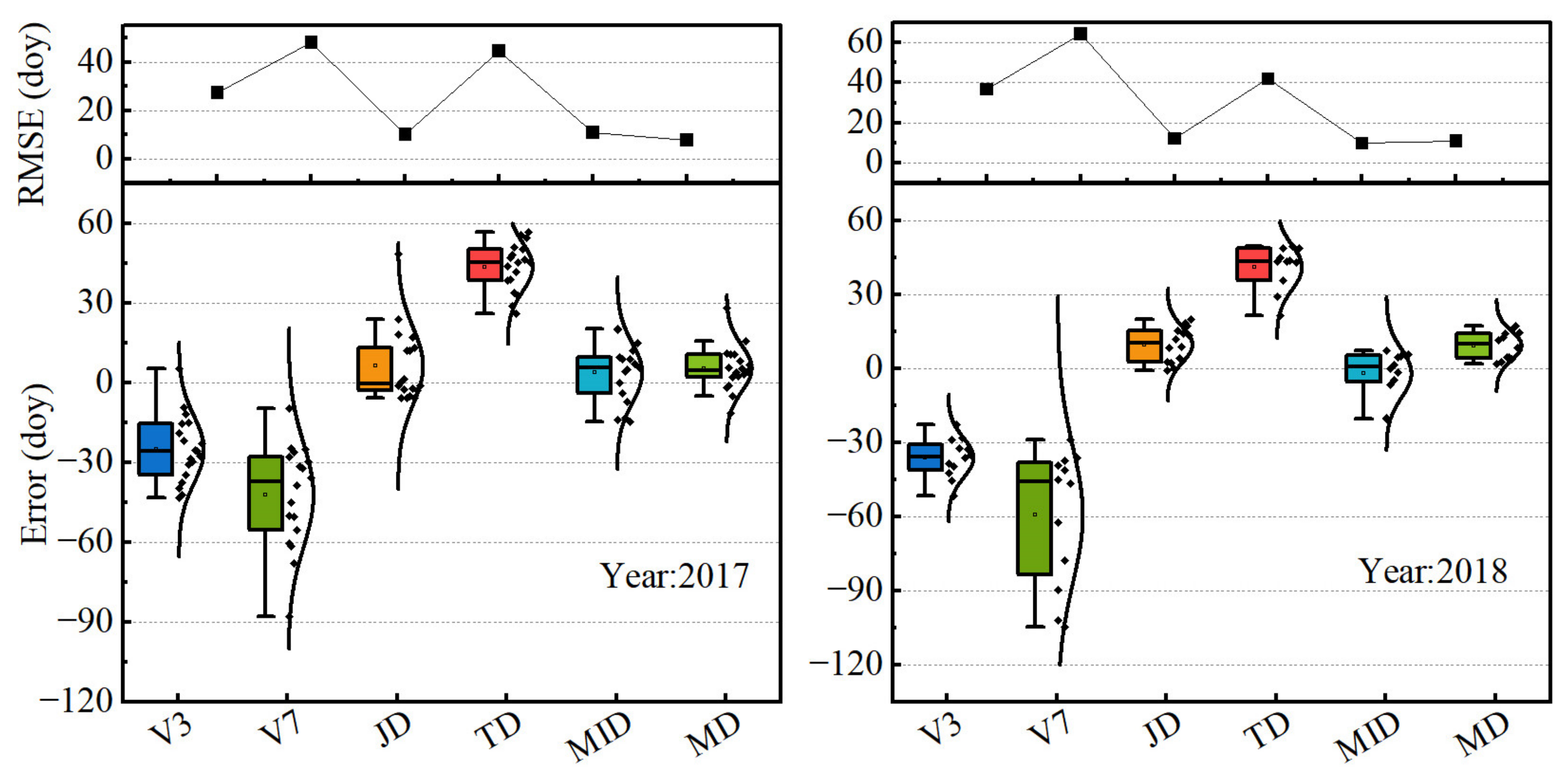
Figure 1. Maize distribution in the study area [41], 2017. The blue and red dots show the spatial distribution of Agricultural Meteorological Stations (AMSs), and the numbers above each station represent the coded name.
Remotesensing 16 00826 g001
Figure 2. Image number spatial distribution of Sentinel-1 and Sentinel-2.
Remotesensing 16 00826 g002
Figure 3. The framework for deriving maize phenology on a regional scale using Sentinel-1 time series.
Remotesensing 16 00826 g003
Figure 4. Sentinel-1 scattering mechanism in different phenological stages of maize. CR value is extracted from the real Sentinel-1. The maize plant graph depicts maize morphology at various phenological stages. They correspond to the CR of each phenological stage. The yellow dotted line divides the maize plants at various stages. ( A and x p are the two variables for calculating the threshold).
Remotesensing 16 00826 g004
Figure 5. CR, VH, and VV in different incident angles. (ac) present CR, VV, and VH scatter plots of site 50,742; (df) present CR, VV, and VH scatter plots of site 50,879; (gi) present CR, VV, and VH scatter plots of site 50,756, (jl) present CR, VV, and VH scatter plots of site 50,739; and (mo) present CR, VV, and VH scatter plots of site 50,954.
Remotesensing 16 00826 g005aRemotesensing 16 00826 g005b
Figure 6. Correlation of VH, VV, and CR with precipitation (Pre), average wind speed (AWS), maximum wind speed (MWS), and incidence angle (Angle). (a) presents V3, (b) presents V7, (c) presents JD, (d) presents TD, (e) presents MID, and (f) presents MD. “*” is significant at the 0.05 level, “**” is significant at the 0.01 level, and “***” is significant at the 0.001 level.
Remotesensing 16 00826 g006
Figure 7. Time series of VH, VV, CR, NDVI, and EVI on maize test sites in 2017. The error bars along the y-axes represent the uncertainty (i.e., standard deviation) of VH, VV, CR, NDVI, and EVI.
Remotesensing 16 00826 g007
Figure 8. The percentage of CR value in each phenological stage to the CR amplitude in entire growing season. The red shading is the 95% forecast band. The difference represents the difference between the CR value and the minimum value at each phenological stage. k represents the optimal threshold for detecting each phenological stage.
Remotesensing 16 00826 g008
Figure 9. RMSE of different percentages of growing season amplitude. The 0.1, 0.2, 0.3, 0.4, 0.5, 0.6, 0.7, 0.8, and 0.9 represent the percentages of the growing season amplitude. The dotted line represents the RMSE from the threshold, which is determined by the adaptive dynamic threshold method.
Remotesensing 16 00826 g009
Figure 10. Relationship between ground observation data and the detected phenology by the adaptive dynamic threshold in 2017 and 2018. The p represents the significance level.
Remotesensing 16 00826 g010
Figure 11. Comparison error and RMSE between ground observation phenology and detection phenology. The whisker is the 95% confidence interval.
Remotesensing 16 00826 g011
Figure 12. Average precipitation in Heilongjiang Province in 2017 (a) and 2018 (b). Different colored rectangular boxes represent various phenological stages. Blue box: V3; Green box: V7; Orange box: JD; Red box: TD; Cyan box: MID; Brown box: MD.
Remotesensing 16 00826 g012
Figure 13. Scatter plots of phenological detection errors by Sentinel-1 and Sentinel-2. (a) represents phenological detection errors in 2017; (b) represents phenological detection errors in 2018.
Remotesensing 16 00826 g013
Figure 14. Comparing the detection of spring maize phenology in 2017 and 2018 using adaptive dynamic thresholds. (a,c,e) represent detected JD, MID, MD in 2017; (b,d,f) represent detected JD, MID, MD in 2018. (a1a4) represent detected JD in 2017 at sites 50,739, 50,858, 50,867, and 50,875; (b1b4) represent detected JD in 2018 at sites 50,739, 50,858, 50,867, and 50,875; (c1c4) represent detected MID in 2017 at sites 50,739, 50,858, 50,867, and 50,875; (d1d4) represent detected MID in 2018 at sites 50,739, 50,858, 50,867, and 50,875; (e1e4) represent detected MD in 2017 at sites 50,739, 50,858, 50,867, and 50,875; (f1f4) represent detected MID in 2018 at sites 50,739, 50,858, 50,867, and 50,875.
Remotesensing 16 00826 g014aRemotesensing 16 00826 g014b
Figure 15. Spatial distribution map of growing degree days (GDDs) and sowing dates in 2017 (a) and 2018 (b).
Remotesensing 16 00826 g015
Table 3. The RMSE between the results of Sentinel-2, Sentinel-1 and ground observation data in each phenological stage (n is the number of AMSs). The year 2017&2018 represents the average RMSE over the past two years.
YearDataV3V7JDTDMIDMD
2017 (n = 20)Sentinel-29.11121.1211.5879.1619.3817.51
Sentinel-127.3348.1710.2444.5710.897.87
2018 (n = 15)Sentinel-211.8514.9311.5716.9812.488.09
Sentinel-136.8264.5711.9642.089.7310.94
2017&2018Sentinel-210.4868.0311.5848.0715.9312.80
Sentinel-132.0756.3711.1043.3310.319.41
Disclaimer/Publisher’s Note: The statements, opinions and data contained in all publications are solely those of the individual author(s) and contributor(s) and not of MDPI and/or the editor(s). MDPI and/or the editor(s) disclaim responsibility for any injury to people or property resulting from any ideas, methods, instructions or products referred to in the content.

