Abstract
The digital elevation model (DEM) and its derived morphometric factors, i.e., slope, aspect, profile and plan curvatures, and topographic wetness index (TWI), are essential for natural hazard modeling and prediction as they provide critical information about the terrain’s characteristics that can influence the likelihood and severity of natural hazards. Therefore, increasing the accuracy of the DEM and its derived factors plays a critical role. The primary aim of this study is to evaluate and compare the effects of resampling and downscaling the DEM from low to medium resolution and from medium to high resolutions using four methods: namely the Hopfield Neural Network (HNN), Bilinear, Bicubic, and Kriging, on five morphometric factors derived from it. A geospatial database was established, comprising five DEMs with different resolutions: specifically, a SRTM DEM with 30 m resolution, a 20 m resolution DEM derived from topographic maps at a scale of 50,000, a 10 m resolution DEM generated from topographic maps at a scale of 10,000, a 5 m resolution DEM created using surveying points with total stations, and a 5 m resolution DEM constructed through drone photogrammetry. The accuracy of the resampling and downscaling was assessed using Root Mean Square Error (RMSE) and mean absolute error (MAE) as statistical metrics. The results indicate that, in the case of downscaling from low to medium resolution, all four methods—HNN, Bilinear, Bicubic, and Kriging—significantly improve the accuracy of slope, aspect, profile and plan curvatures, and TWI. However, for the case of medium to high resolutions, further investigations are needed as the improvement in accuracy observed in the DEMs does not necessarily translate to the improvement of the second derivative morphometric factors such as plan and profile curvatures and TWI. While RMSEs of the first derivatives of DEMs, such as slope and aspect, reduced in a range of 8% to 55% in all five datasets, the RMSEs of curvatures and TWI slightly increased in cases of downscaling and resampling of Dataset 4. Among the four methods, the HNN method provides the highest accuracy, followed by the bicubic method. The statistics showed that in all five cases of the experiment, the HNN downscaling reduced the RMSE and MAE by 55% for the best case and 10% for the worst case for slope, and it reduced the RMSE by 50% for the best case of aspect. Both the HNN and the bicubic methods outperform the Kriging and bilinear methods. Therefore, we highly recommend using the HNN method for downscaling DEMs to produce more accurate morphometric factors, slope, aspect, profile and plan curvatures, and TWI.
1. Introduction
Digital elevation models (DEMs), which were introduced in the late 1950s, have been widely utilized in various applications dealing with the Earth’s surface, including, but not limited to, hydrology, geology, cartography, geomorphology, engineering, and landscape architecture [1,2,3]. DEMs have especially been extensively utilized in the last decade for accurate modeling and predicting natural hazards, including landslide [4,5], soil erosion [6,7], flood [8,9], and sea level rise assessment [10,11]. Herein, the accurate prediction of natural hazards refers to the ability to predict the occurrence, severity, and location of natural hazards with high accuracy.
Literature review shows that the accuracy of natural hazard prediction is significantly dependent on both the methods employed for modeling and the data used [12,13], which includes the DEM and its derived topographic or morphological factors, such as slope angle, slope aspect, plan curvatures, profile curvatures, and topographic wetness index (TWI). Basically, high-resolution DEMs are commonly assumed to provide superior results in natural hazard mapping. A higher accuracy DEM can provide more precise information on the extracted topographic factors such as slope, aspect, plan curvature, profile curvature, and TWI, resulting in more accuracy in the applications [14]. In other words, higher accuracy input DEM can improve the accuracy of these applications by providing more detailed information on topographic factors.
DEM data, mostly in grid raster, are acquired using different methods such as ground surveying, photogrammetry, optical and radar remote sensing, light detection and ranging (LiDAR). These data, therefore, are available at various resolutions and accuracy depending on the data acquisition methods [15]. The resolution may range from a very high of 0.5 m to 5 m collected by the LiDAR or ground survey to a medium of 30 m by Advanced Spaceborne Thermal Emission and Reflection Radiometer (ASTER) and 90 m by Shuttle Radar Topography Mission (SRTM) data. It is apparent that DEMs created using total stations, drone photogrammetry, or LiDAR have demonstrated the highest level of accuracy [16,17,18]. However, these accurate DEMs are not always available in the areas of interest. Therefore, improving the accuracy of the DEMs and their morphometric factors through sub-pixel methods and interpolation techniques may be an alternative to obtaining the DEM and its derived morphometric factors at an acceptable level of accuracy.
Numerous methods and techniques have been proposed to increase the DEM accuracy for natural hazard predictions [14,19]. Some of these are based on the down-sampling of DEM to different resolutions, and they use these DEMs to calculate the input factors for natural hazard models in different regions [20]. Thus, the accuracy and grid DEM resolution can be increased using resampling and downscaling methods [19,20]. The common approaches for downscale resampling are bilinear, bi-cubic, and Kriging [21]. The main advantage of these methods is that they do not require prior DEM data at different resolutions for training and are computationally efficient. However, accuracy may not be satisfactory in some cases.
More recently, a number of sophisticated deep learning artificial intelligence models, such as deep residual networks [22], Recursive Sub-Pixel Convolutional Neural Networks [23], Laplacian of Gaussian Super-resolution [24], Reconstruction Network Combining Internal and External Learning [25], Super-Resolution with Generative Adversarial Network [26] have been proposed. These methods are mostly based on approaches proposed for image super-resolution [22,23,24,25,26]. The result shows that the DEM accuracy has improved regarding root mean square error (RMSE) and the closeness to the reference data [19,20]. However, although showing potential for improvement of super-resolved DEMs’ accuracy, applying these methods still required large amounts of training data and very high-capacity hardware to build complex neural network models.
In recent research, we proposed a method for downscaling DEM using Hopfield Neural Network (HNN) [20] with promising results. This method not only improves the accuracy of DEMs but also is computationally efficient and can be performed on personal computers without incurring high costs. However, the extent to which DEM resampling approaches can improve the accuracy of derived morphometric factors, i.e., slope, aspect, plan curvature, profile curvature, and topographic wetness index (TWI), is still unknown.
This research aims to address this gap in the literature by assessing and comparing HNN, bilinear, bi-cubic, and Kriging methods regarding the enhancement of the accuracy of the five morphometric factors mentioned above through up-sampling and downscaling of DEMs across various resolutions. Herein, five DEMs with different resolutions were used for testing such as SRTM DEM with 30 m resolution, 20 m resolution DEM generated from topographic maps at a scale of 50,000, 10 m resolution DEM generated from topographic maps at a scale of 10,000, 5 m resolution DEM constructed using surveying points with total stations, and 5 m resolution DEM built using drone photogrammetry.
2. Method and Data Used
2.1. Method Used
2.1.1. Hopfield Neural Network
The Hopfield Neural Network (HNN) is a recurrent artificial neural network that was proposed by John Hopfield in 1982 [27]. This method operates based on the principle of maximizing spatial dependence or similarity among adjacent pixels within an image. For downscaling of the DEM in this research context, the spatial dependence is interpreted as a goal function as
where is the average value computed from the surrounding pixels to the pixel (i,j), h is the distance from the pixel (i,j) to the surrounding pixel is an elevation correction value of pixel (i,j) at the iteration u, and is the elevation value of the iteration u − 1.
In HNN downscaling, each sub-pixel or pixel at a higher resolution is represented by a neuron, and the whole DEM image is a panel of neurons.
Together with the goal function, an elevation constraint function is as follows:
where is the elevation value of pixel (x,y) in the original image, is the output (elevation) value of the sub-pixel (p,q) in the newly generated image covered by pixel (x,y), and f is the zoom factor.
If the average of the elevation values of all sub-pixels within a pixel is smaller than the , then the elevation values of all sub-pixels within the footprint of pixel (x,y) are increased.
In contrast, when the average of the elevation values of all sub-pixels within a pixel (x,y) is larger than the , a value is subtracted from the output value of the neuron (p,q).
The HNN network runs in an iterative process until the energy E value is minimized as
2.1.2. Bilinear Interpolation Method
Bilinear interpolation is a conventional method used to interpolate pixel values based on the weighted average of neighboring pixels [28]. This technique assumes that the pixel intensity changes linearly across the image, and its value is computed using the formula as follows:
where is the value of the pixel, ; f(0,0), f(1,0), f(0,1), and f(1,1) are the values of four surrounding pixels (0,0), (1,0), (0,1), and (1,1) of the pixel . In the case of resampling of the DEM, represents the elevation of the pixel .
2.1.3. Bi-Cubic Interpolation Method
The bi-cubic interpolation method uses the closest 4 × 4 surrounding pixels for a total of 16 pixels to calculate the value of the pixel at the location (x,y) [29]:
where is the value (elevation) of the pixel ; is the value of the surrounding pixel (i,j) of the original image used to calculate with i = 0,..., 3, j = 0,..., 3; and is weight value which is computed using the distances from pixel to the pixel (i,j) at the original image.
2.1.4. Kriging Interpolation Method
Kriging interpolation is a method of interpolation based on the spatial correlation between sampled points [30]. Kriging consists of two steps. The first step is to determine the spatial covariance structure of the sampled points by fitting a variogram. The second step is to derive a weight matrix from the covariance structure obtained in the first step and use this weight matrix to calculate the value (elevation) of the pixel (x,y). The computation of of Kriging is similar to that of bi-cubic resampling as follows:
However, the calculation of weight values is based on a different process using the covariance structures obtained from the surrounding pixels.
2.2. Data Used
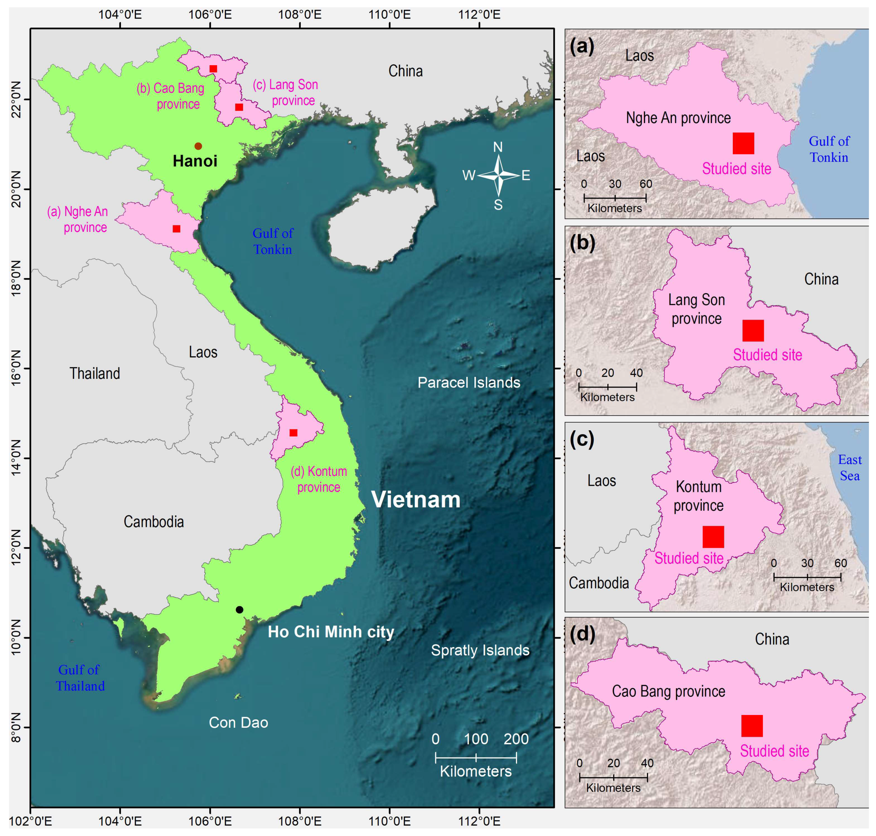
In this research, five DEM datasets (Table 1) of different areas in Vietnam and at a variety of resolutions were used. The locations of these datasets are presented in Figure 1.

Table 1.
DEM datasets at different spatial resolutions and locations.

Figure 1.
Four datasets (a) DEM 20 m and 30 m in Nghe An Province; (b) DEM 5 m in Lang Son Province; (c) DEM 10 m in Kon Tum Province; (d) DEM 5 m in Cao Bang Province.
Dataset 1 is a 30 m DEM obtained from the Shuttle Radar Topography Mission (SRTM) and downloaded from USGS EarthExplorer (accessible via https://earthexplorer.usgs.gov, accessed on 2 September 2023). This dataset covered an area of about 3.5 km by 3.5 km and is located at 18°58′57.03″N, 105°22′44.87″E in Yen Thanh District, Nghe An Province, in North Central Vietnam. This area was selected because the vegetation covers were very low, and its effect to the elevation accuracy of SRTM data was minimized. This DEM is used to examine the impact of the resampling and downscaling of DEM from lower resolution to 30 m resolution. To obtain the DEM at low resolution, the 30 m DEM was upscaled to the resolution of 90 m for evaluation on the impact of resampling and downscaling.
Dataset 2 is a DEM obtained from the same location as the first dataset. This DEM was generated by Kriging (ordinary Kriging) interpolation of contours in topographic maps with a scale of 1:10,000. The original DEM had a spatial resolution of 20 m, but it was upscaled to 60 m by averaging the elevation values of 20 m pixels that were within the boundaries of the degraded 60 m pixels.
Dataset 3 was acquired using ground surveying in Lang Son Province of Vietnam. The test field is situated in Mai Pha Ward, Lang Son City, and covers an area of approximately 200 m by 200 m. In order to create a gridded 5 m DEM dataset for reference purposes, a total of 533 elevation points were measured and processed with Kriging interpolation. The accuracy of the reference DEM was determined by evaluating its Root Mean Square Error (RSME) with 234 validation points. The vertical accuracy of the elevation points measured by Topcon total station is 0.05 m (Vertical and horizontal accuracy of angle measurement is 5″ and accuracy of distance measurement is 5 mm).
Dataset 4 was created from contour data in Dac Ha district, Kontum Province, Vietnam, at the location of 14.671794°N and 107.967292°E. The survey area covers an approximate area of 6.6 km by 6.6 km. A DEM with a resolution of 10 m was generated from the original contour data, which was obtained at 5 m intervals. This 10 m DEM was used as the reference dataset. In order to produce coarse 30 m spatial resolution input data for resampling and downscaling, 10 m interval contours were interpolated from the same area.
Dataset 5 has an area of 1.4 km × 1.4 km and was obtained using an unmanned aerial vehicle in Cao Bang Province. The DJI Phantom 4 RTK was used with a flying height of 150 m to generate two sets of DEMs, as in Table 1. The 5 m and 20 m DEMs were generated from the 2000 and 500 elevation point datasets with accuracy of 2.2 m and 0.5 m, respectively (see Table 1).
2.3. Morphometric Factors
In this analysis, four morphometric factors were considered: slope, aspect, plan curvature, profile curvature, and Topographic Wetness Index (TWI).
2.3.1. Slope and Aspect
The most utilized algorithms calculate slope and aspect from a Digital Elevation Model (DEM) using a 3 × 3 cell neighborhood. Several methods of calculating the slope and aspect from the 3 × 3 cell window include the Maximum Slope Method, Maximum Downhill Slope Method, Quadratic Surface Method, and Neighborhood Method [31]. Comparing these methods using a standard Morison’s surface, Jones [32] indicated that the method of Horn is suitable for calculating both slope and aspect from DEM. The slope and aspect calculation in this paper is implemented using this method which is incorporated in the SAGA tools in QGIS software (Version 3.14).
2.3.2. Plan Curvature and Profile Curvature
Plan and profile curvatures are conditional factors used in many different models for landslide, hydrological and biophysical property modeling, and landform classification. The two mostly used curvatures are plan curvature and profile curvature [33,34]. These curvatures are the second-order derivatives of the topography [35]. The method for plan and profile curvatures from DEM in this paper was proposed by Zevenbergen and Thorne [36] and deployed as a tool in SAGA using QGIS.
2.3.3. Topographic Wetnet Index
The Topographic Wetness Index (TWI) presents the potential for water to accumulate in a given location based on the topography of the area. TWI is a measure of soil moisture based on terrain features derived from a DEM. The calculation of TWI is usually based on a gridded DEM, and the value of TWI at a point [37,38] is computed as follows:
where a is the upslope contributing area per unit contour length (or Specific Catchment Area, SCA) and β is the local slope gradient for reflecting the local drainage potential. The calculation of a and the estimation of tanβ algorithms exert an impact on the TWI value [38].
2.4. Accuracy Assessment
The accuracy assessment of slope, aspect, plan curvature, profile curvature, and TWI obtained from different DEMs commonly relies on the root mean square error (RMSE) [39]. By comparing the RMSE among different DEMs, it is possible to evaluate the differences in the topographic factors derived from them.
In addition to the RMSE, other statistics were also used. For slope evaluation, statistics such as Mean Absolute Error (MAE), or the minimum, maximum, and mean values, were used to provide insight into the range of values and the trends or patterns in the slope. The evaluation of the aspect was based on RMSE and the categories of aspect value difference, which reflects the change of slope direction, which may substantially affect the natural process and hazard modeling. The assessment of plan and profile curvatures was implemented using the percentages of correct classification of curvature features such as concave, convex, and zero curvature.
Together with the above-mentioned parameters, the histograms of the topographic factors are also used for evaluation. The histograms may show differences or closeness in the distribution of slopes at different resolutions and accuracies or visually present the trends and distributions of their values.
3. Results and Discussion
3.1. Results of Downscaling and Resampling of the Digital Elevation Model
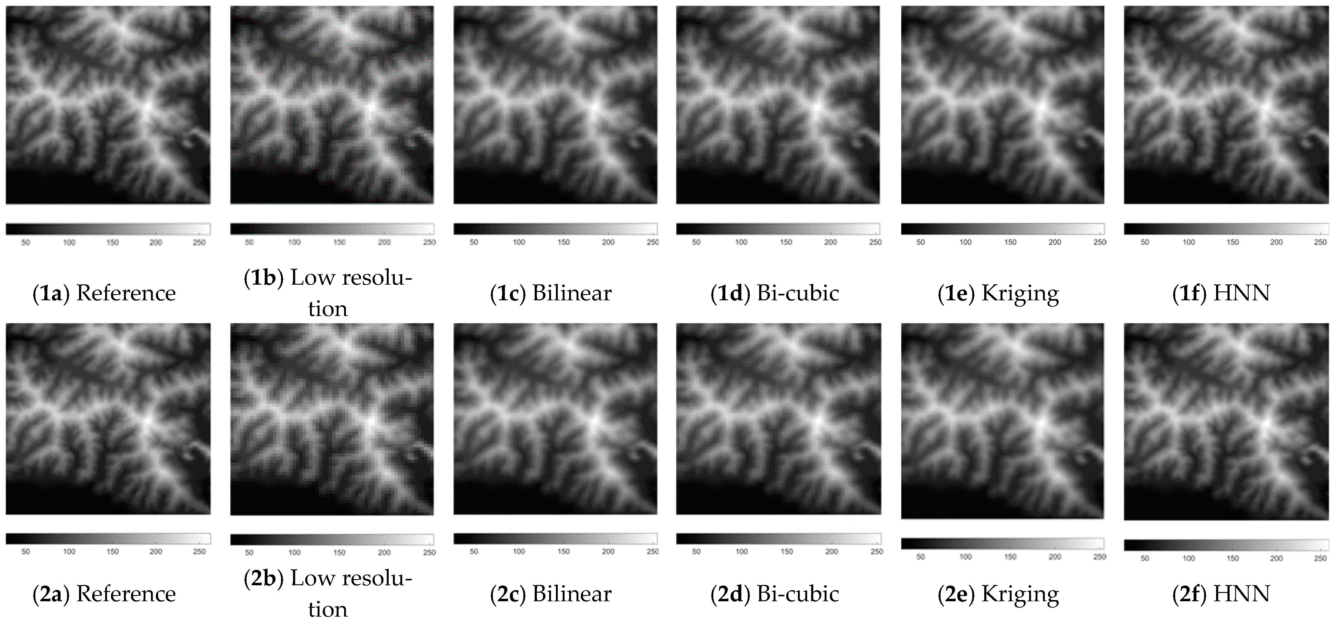
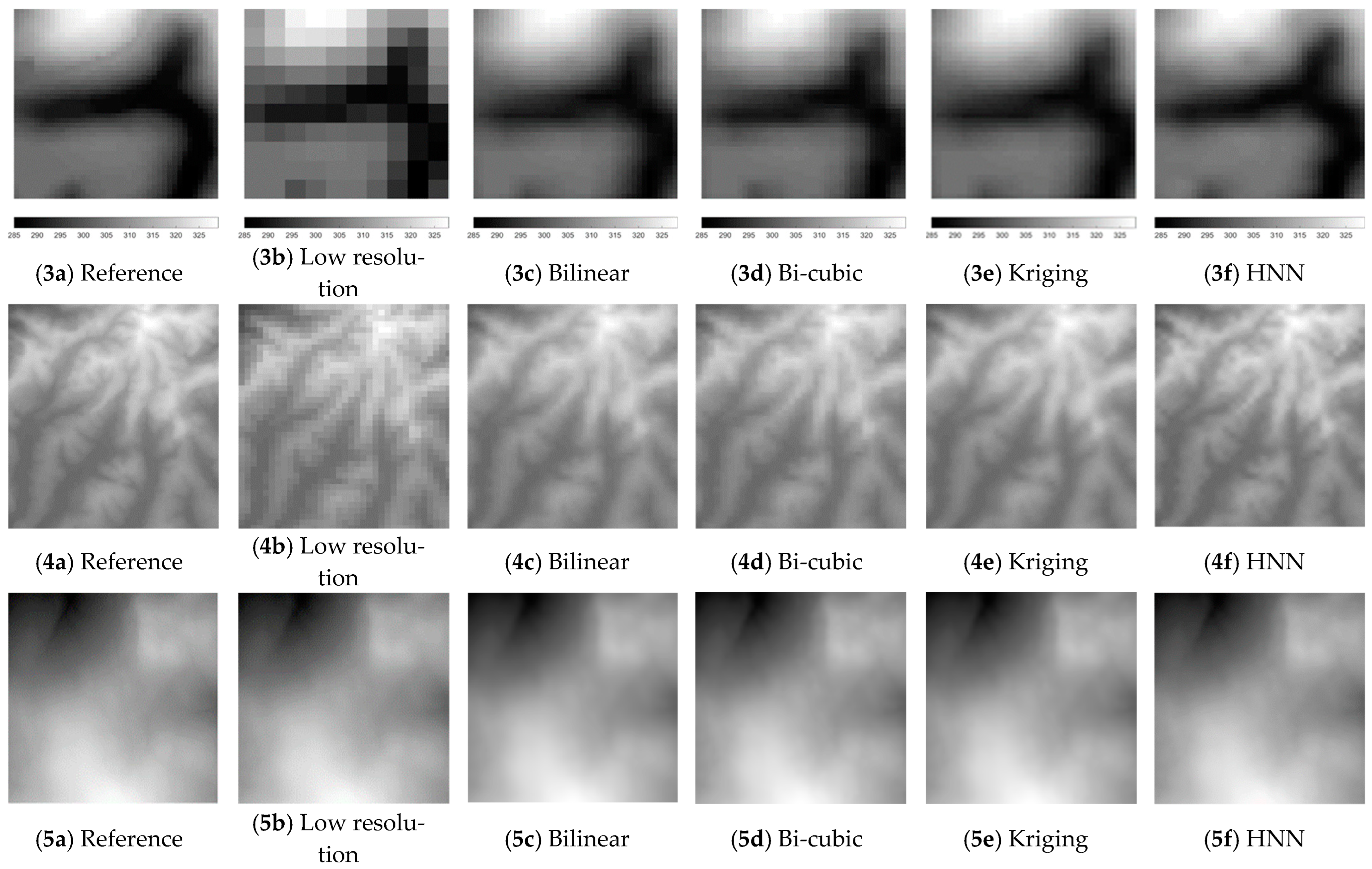
In order to evaluate the impacts of up-sampling and downscaling on the morphometric factors, the DEM experiment datasets were downscaled using four approaches: bilinear, bi-cubic, Kriging, and Hopfield Neural Network. The zoom factors were used as presented in Table 1. These zoom factors were used with the aims of evaluating the impact of up-sampling and downscaling from coarse resolution to medium resolution, as in the cases of 90 m DEMs to 30 m DEMs and 60 m DEM to 20 m DEM, and from medium resolution to fine resolution, as in the cases of 30 m DEMs to 10 m DEMs, and 20 m DEMs to 5 m DEMs. The result of the downscaled DEMs is presented in Figure 2, and the RMSE of each resampled DEM against its reference DEM is presented in Table 2.
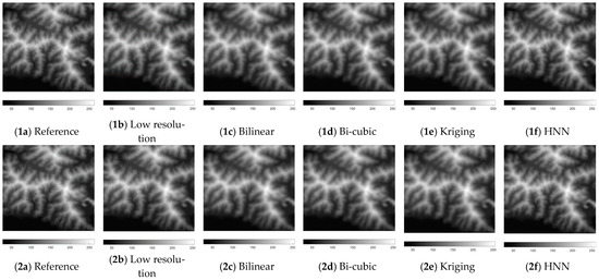
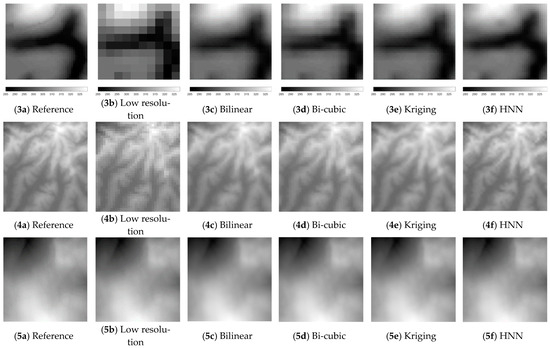
Figure 2.
Resampling and downscaling results: (1a–1f): Reference, Input and downscaled and resampled DEMs in Dataset 1; (2a–2f): Reference, Input and downscaled and resampled DEMs in Dataset 2; (3a–3f): Reference, Input and downscaled and resampled DEMs in Dataset 3; (4a–4f): Reference, Input and downscaled and resampled DEMs in Dataset 4; (5a–5f): Reference, Input and downscaled and resampled DEMs in Dataset 5.
Table 2.
RMSE of the resampled DEMs.
3.2. Slopes of the Resampled and Downscaled Digital Elevation Models
Evaluation of the effect of the resampling and downscaling of DEM to topographic factors is conducted based on both visual analysis and quantitative analysis. The visual analysis is implemented using histograms of the slope values obtained by bilinear, bi-cubic, Kriging, and HNN approaches, as presented in Figure 3.
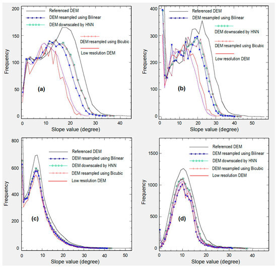
Figure 3.
Histograms of the slopes obtained from the (a) Dataset 1: 30 m DEM in Nghean; (b) Dataset 2: 20 m DEM in Nghean; (c) Dataset 4: 10 m DEM in Daklak; (d) Dataset 5: 5 m DEM in Caobang.
Comparisons of slopes generated from resampled and downscaled DEMs showed that resampling and downscaling could improve the accuracy of slopes. Due to the smoothing effect, the slopes calculated from DEMs at low resolutions are always lower in comparison with those calculated from higher-resolution DEMs [15]. This trend is evident in the histograms of slopes obtained from referenced DEMs, original DEMs, and resampled DEMs using various methods, as shown in Figure 3. Applying the resampling methods to increase the resolution of DEMs, the number of points with higher slopes increased and approached those observed in the referenced DEMs as a result.
The increasing slope angle after using resampling and downscaling methods can be easily seen in the high slope values larger than 10° especially in slope histograms of DEM at medium resolutions of Dataset 1 (Figure 3a) and Dataset 2 (Figure 3b). The data in these figures revealed that the number of pixels exhibiting slope angles ranging from 10° to 40° increased when utilizing Kriging interpolation, bi-cubic resampling, and HNN downscaling in comparison to low-resolution DEMs. For the DEM at higher resolution, as in Figure 3c, 3d resampling approaches do not increase the slope values as much as for the DEM of medium resolution. This may be explained by the fact that in cases where the original DEMs have resolutions of 20 m or 30 m, the smoothing effect on the topography is not as severe as in cases where of original DEMs have resolutions of 60 m or 90 m.
Visual analysis of the histogram in Figure 3 shows that the resampling methods used in this research, bi-cubic and HNN are evidently superior to Kriging and bilinear resampling. By looking at the histograms in Figure 3, it is possible to see that in most of the cases, the histograms of bilinear resampling DEM’s are very close to those of the original low resolutions, while the histograms of Kriging, bi-cubic, and HNN are close to each other and closer to the slopes calculated from referenced DEMs.
Quantitative analysis in Table 3 shows the changes in slope angles due to the resampling effects. For the medium resolutions, the increase in slope angles can be seen in the maximums and means of the slopes in both Dataset 1 (90 m to 30 m DEMs) and Dataset 2 (60 m to 20 m DEMs). While the maximum and mean values of slopes in low-resolution data are considerably smaller than those in high-resolution data, the application of resampling techniques significantly increased these statistics. Except for the Kriging interpolation, all of the other resampling approaches increase the maximum values of slopes between 8° to 13° from the original 60 m and 90 m DEMs, which had maximum slope values of 24.40° and 32.91°, respectively, to make them closer to the maximum slope values of 44.49° and 57.57° of the fine 20 m and 30 m reference DEMs, respectively. Similarly, the mean values of resampled slope data increase by around 2° to 3° compared to the original low-resolution slope data, making them just approximately 1.5° lower than the reference high-resolution slopes for both medium-resolution datasets.
Table 3.
Statistics on the slopes generated from DEMs created from the resampling and downscaling methods.
Resampling of DEM from medium resolution to high resolution has similar impacts as of the medium resolution when the maximum and mean slopes were considered. In all three datasets of high-resolution DEMs shown in Table 2, except for the bilinear and Kriging methods in the Langson 5 m dataset (Dataset 3), both the maximum and mean slope values were observed to increase. However, the increase is not as significant as that seen in the medium-resolution data, with maximum slopes increasing by approximately 5° to 7° and mean slopes increasing by 0.5° to 1.5°.
Evaluation of the DEM resampling impacts on the accuracy of the slopes was also implemented using RMSE and MAE. These two statistics show the closeness of the two datasets. The statistics in Table 2 demonstrate that resampling techniques can make the slopes created from the coarse DEMs significantly closer to those from the fine reference DEM. The increase in slope accuracy achieved through downscale resampling from coarse-resolution DEMs to medium-resolution DEMs is greater than that achieved through downscaling from medium-resolution DEMs to high-resolution DEMs. In both cases of downscale resampling from 90 m to 30 m and from 60 m to 20 m, an average reduction of approximately 50% in RMSE is observed. The most significant improvement is seen in the case of HNN downscaling, where the RMSE is reduced from 6.98° and 7.18° of coarse resolution slope data to 3.10° and 4.18° of HNN downscaled slope data, respectively. In addition, bi-cubic resampling is also a valuable approach for slope improvement with an RMSE of 3.27° for a 30 m DEM case and 4.13° for a 20 m DEM case. Comparing these two approaches, bilinear and Kriging are not very impressive. The reduction in RMSE of bilinear resampling is around 35% to 4.100 and 4.86° for 90 m to 30 m cases and 60 m to 20 m cases, respectively. The RMSE of Kriging even slightly increased in the case of the 60 m to 20 m.
The evaluation based on MAE shows the same results as the RMSE. The reduction of MAE is from 5.55° to 2.46° for bi-cubic and 2.33 m for HNN downscaling in the 90 m to 30 m resampling case. For the case of downscale resampling from 60 m to 20 m, the MAE of the slopes reduced by almost 50% from 5.41° to 2.80° and 2.86° for bi-cubic and HNN downscaling, respectively. However, the resampling using bilinear and Kriging does not give the same good results as bicubic and HNN downscaling in terms of MAE. The reduction in MAE is observed with bilinear resampling in both datasets but not with Kriging in the case of downscale resampling from 60 m to 20 m.
In three datasets of downscaling from medium to high resolutions (Dataset 3, Dataset 4, Dataset 5), the statistics show less impressive results than that of the coarse-to-medium downscaling. The RMSE and MAE reductions of slopes by resampling are only from 6% to 40% compared with the slopes obtained from original low-resolution data. The best downscaling methods are still HNN downscaling and bi-cubic. The HNN downscaling is slightly better than bi-cubic in all three cases with RMSE of 7.60°, 1.42°, and 2.58° for HNN downscaling in Dataset 3, Dataset 4, and Dataset 5, respectively, compared to RMSE of 7.60°, 1.51°, and 2.61° for bi-cubic resampling in Dataset 3, Dataset 4, and Dataset 5, respectively. The statistics of MAE also yield the same results for the HNN downscaling and bi-cubic resampling with MAE values of 5.22°, 0.86°, and 1.80° for Dataset 3, Dataset 4, and Dataset 5, respectively, while the MAE values for the Dataset 3, Dataset 4, and Dataset 5 of the bi-cubic resampling are 5.77°, 0.88° and 1.87°, respectively.
Among the resampling methods for three cases of medium to high resolutions, the bilinear resampling produced the worst results with values of MAE of 6.09 m in Dataset 3, and RMSE and MAE of 3.27° and 2.16°, respectively, in Dataset 5. These results are even worse than those of the low resolutions slope with the values of MAE of 5.97° in the case of Dataset 3, RMSE of 2.92° and MAE of 2.08° in the case of Dataset 5. This means the bilinear resampling and Kriging interpolation of DEM are not always reliable for effectively improving the quality of slope data in many cases. In contrast, the bi-cubic and HNN downscaling are viable methods to make the slope created from low-resolution DEMs closer to those produced from higher spatial resolution DEMs.
3.3. Aspects of the Resampled and Downscaled Digital Elevation Models
Although aspect is sometimes considered an indirect factor to the earth process modeling, it directly impacts the distribution of solar radiation, temperature, and soil moisture over the terrain. Specifically, aspect represents the orientation of a slope relative to the sun, and this determines the amount of solar radiation received by the area, which subsequently affects its temperature and moisture conditions and the vegetation patterns, soil features, and erosion processes across the landscape.
Aspect is measured clockwise from the north and takes values between 0 and 360 degrees. Depending on the intervals used, aspects of different values can be categorized into groups. For instance, slope directions can be classified into four geographical directions, namely North, South, East, and West, using 90-degree intervals. Alternatively, 45-degree intervals can be used to divide slope directions into eight categories: North, North-East, East, South-East, South, South-West, West, and North-West. Depending on the scale and resolutions of the original DEMs, the different extent of changes in aspect may influence the accuracy of the earth process modeling. Therefore, in this paper, in addition to using statistics such as RMSE, the evaluation of aspect is also based on the percentages of groups of aspect value difference within intervals such as 0–10°, 10–20°, 20–45°, 45–90° and 90–180°. The differences in aspect values are calculated by comparing the aspects of the original low-resolution DEMs and resampled DEMs with the aspects obtained from the reference DEMs at high resolutions. For example, if the calculated aspect value of a pixel in 20 m resampled DEM is 40° and in reference DEM is 55° the aspect difference is 15°, and the pixel is located in the 10–15° difference group. The percentage is calculated based on the fraction of the total number of pixels belonging to a group and the total number of pixels. The results on RMSE and percentages of each group of aspect differences are presented in Table 3.
The resampling approaches improved the accuracy of the aspect when they downscaled the DEMs from low to medium resolutions, as shown by the RMSE values in Table 3. The aspects of the original low-resolution DEMs at 60 m (Dataset 2) and 90 m (Dataset 1) differ remarkably from the reference DEMs at 20 m and 30 m, with RMSE values of 40.73° and 34.45°, respectively. The resampling approaches improved the aspects significantly, lowering the RMSE values by half to around 20.21° for the bi-cubic resampled and HNN downscaled DEMs at 30 m resolution. For the case of Dataset 2, the improvement is also very impressive with RMSE of the aspects produced by 20 m bi-cubic resampled and HNN downscaled DEMs of 20.41° and 20.35°, respectively. The other resampling techniques, such as bilinear and Kriging, although not as good as bi-cubic and HNN, still enhance the accuracy of the resulting aspects. The RMSEs of aspects of 23.88° and 32.20° for 30 m bilinear resampled DEMs and Kriging interpolation, respectively, and 31.91° and 31.91° for 20 m bilinear resampled and Kriging interpolation, respectively, are still much smaller than those of original one.
The impact on accuracy improvements of aspect by DEM resampled from medium to high resolutions in Dataset 3, Dataset 4, and Dataset 5 is not as great as in Dataset 1 and Dataset 2. The improvement in RMSEs is less than 10° for all three datasets. Especially for the DEMs downscaled by four times in Dataset 5, the improvement in aspect accuracy is less than 20, which may not be significant enough for some applications, such as landslide modeling, to result in an overall accuracy improvement.
To evaluate the impacts of resampling on aspect values and, eventually, the accuracy of earth process modeling or natural hazard prediction, it is necessary to analyze the characteristics of aspect difference presented in Table 4. In this table, the percentages of the different groups show that the aspect calculated from the low-resolution DEMs at 90 m and 60 m in Dataset 1 and Dataset 2 differs significantly from the aspect calculated from reference DEM at 30 m and 20 m. Only 27.60% and 33.66% of the aspect calculated from low-resolution DEM of 90 m and 60 m, respectively, are in the group of difference in aspect value of 0–10°, which means the aspect values are very close to the aspect calculated from the higher resolution DEMs. Conversely, the percentages of the 45–90° group and the 90–180° group are 13.76% and 4.66%, respectively, for the aspect from 90 m DEM and 9.24% and 2.78%, respectively, for the aspect from 60 m DEM. If the aspects of two pixels are 90° different, it means that they are facing in opposite directions. Hence, for the pixels located in these groups, the slope directions calculated from low-resolution DEM are completely opposite to the calculated value of the corresponding pixel from the higher-resolution one.
Table 4.
RMSE and percentages of aspect differences within 0–10°, 10–20°, 20–45°, 45–90°, and 90–180°.
Unlike the aspects of the DEMs from Dataset 1 and Dataset 2, most of the aspect values calculated from the medium resolutions at 20 m and 30 m are similar to those computed from the higher resolution DEMs at 5 m and 10 m resolutions in the case of Dataset 3, Dataset 4, and Dataset 5. In all three datasets, over 55% of aspects generated from 20 m or 30 m resolution DEMs are within 10 degrees of the aspects at the same position produced by 5 m or 10 m DEMs.
The discrepancy of aspects computed from DEMs at different resolutions can be partly resolved using resampling approaches. The statistics in Table 3 suggest that resampling approaches can be used in most cases to make the aspects from low-resolution DEMs more similar to those from higher-resolution DEMs. This means the resampling approaches, especially the bi-cubic and HNN downscaling, can effectively improve the accuracy of aspect data derived from low-resolution DEMs. Applying these resampling approaches to DEMs, the percentage of group 0–10° increased approximately twice to 59.63% and 59.93% for Dataset 1 and Dataset 2, respectively, while the percentages of 45–90° and 90–180° groups reduced sharply from 13.76% and 4.66% to 2.50% and 0.80%, respectively, for Dataset 1 and from 9.24% and 2.78% to 3.42% and 0.64%, respectively, for the 60 m Dataset 2. For Dataset 3, Dataset 4, and Dataset 5, the bi-cubic and HNN downscaling are also very effective in improving the accuracy of the aspects. The percentage of the 0–10° group increased from 55.56%, 71.92%, and 55.26% to 57.61%, 86.78%, and 59.85% for Dataset 3, Dataset 4, and Dataset 5, respectively, using bi-cubic and to 60.49%, 87.19%, and 59.64% using HNN downscaling. Furthermore, the application of bi-cubic and HNN can reduce the percentage of aspects in the 45–90° and 90–180° groups by at least one-third, as in Dataset 5 case or maybe higher in Dataset 3 and Dataset 4.
3.4. Plan Curvatures and Profile Curvatures of the Resampled and Downscaled Digital Elevation Models
Plan and profile curvatures are second derivatives of the elevation surface, representing the slope change rate in the directions parallel and perpendicular to the contour lines and profile lines, respectively. The plan and profile curvatures can be calculated using a DEM, and the unit of measure is inverse meter (m−1). In some processes of earth material movement, such as landslides and debris flow, the amount of movement correlates with landforms such as concave and convex, and therefore, it is necessary to determine these landforms (curvature features). The land surface can be classified into concave, zero curvature, and convex landforms based on the values of plan and profile curvatures, which have negative, zero, or positive values. The accurate identification of concave and convex features is crucial for soil and earth movement modeling. A concave feature mistakenly identified as a convex feature may result in an inaccurate prediction of where water will flow and collect. Therefore, in this research, in addition to statistics like RMSE, the assessment of curvature calculation is also based on the correctness of curvature feature recognition. The statistics for this accuracy assessment are the percentages of correct and incorrect curvature features obtained from a DEM against the curvature features produced by the reference DEM at a higher resolution. The RMSE and curvature feature recognition accuracy statistics of all five testing datasets are presented in Table 5.
Table 5.
RMSE of plan and profile curvatures and curvature features recognition accuracy of five testing datasets.
The results based on both RMSEs and curvature features assessment show that the application of DEM resampling from low resolutions to medium resolutions, for example, from DEM 90 m to DEM 30 m or 60 m to 20 m, can improve the accuracy of plan and profile curvatures slightly. Using HNN downscaling, the RMSEs of plan and profile curvatures reduced slightly to 0.01915 m−1 and 0.00125 m−1 from 0.01983 m−1 and 0.00169 m−1, respectively, of original low-resolution DEM for Dataset 1. Moreover, the percentage of incorrect recognition of curvature features such as concave, zero, and convex reduced sharply by approximately 15% for both plan and profile curvatures. In the case of Dataset 2, although the RMSE of HNN downscaling slightly increased for plan curvature, the RMSE of profile curvature and percentages of the incorrect curvature recognition were reduced. Especially, the percentage of correct recognition of the profile curvature feature improved by 30% compared with that of “no resampling” data.
The results of the other resampling methods are not as consistent as those of the HNN downscaling. While the Kriging is not an effective method for downscaling curvatures in all five experiment datasets, as evidenced by both RMSE and curvature feature recognition, the bi-cubic and bilinear resampling approaches are also unreliable. The statistics for all five datasets presented in Table 4 show that while resampling generally improved the curvature accuracy, they do not perform better than “no resampling” in all the statistics. Particularly, in each of the five experiments presented in Table 4, the resampled data is inferior to the original low-resolution DEM in at least one out of the four statistics.
3.5. Topographic Wetness Index of the Resampled and Downscaled Digital Elevation Models
The TWI measures the potential of water accumulation in each pixel on the DEM. High TWI values indicate high soil moisture and low soil stability. Therefore, inaccurate measurement of TWI may lead to false predictions of safe and unsafe landslide areas or soil erosion. In this research, TWI was evaluated based on the RMSE and MAE of TWIs from resampled DEMs against those computed from the reference DEMs, as in Table 6.
Table 6.
RMSE and MEA of Topographic Wetness Index in five experimental datasets.
The results in Table 6 show a good improvement in the TWI values using resampling approaches for the cases of low-to-medium DEM. Both Dataset 1 (90 m to 30 m) and Dataset 2 (60 m to 20 m) showed a significant decrease in both RMSE and MAE values by over 50% compared to “No Resampling”. For Dataset 1, the values reduced from 1.499 and 0.985 to 0.362 and 0.491 for bi-cubic resampling, respectively. For Dataset 2, they reduced from 2.235 and 1.393 to 0.362 and 0.491 for the best resampling method (bi-cubic), respectively. Unlike in the cases of slope and aspect, the HNN downscaling did not perform as well as the other resampling approaches. The bi-cubic and bilinear resampling approaches had the best performance compared to the other methods.
In comparison to the low-to-medium resolution resampled data, the results of TWI calculated from medium-to-high resolution DEMs were found to be less accurate in two out of three datasets, where the TWI values derived from resampled DEM were less accurate than those produced from “no resampling”, as indicated by slightly larger RMSE and MAE values. Only in Dataset 5’s case, the bi-cubic and HNN show a significant reduction of 60% in both RMSE and MAE.
To have a deeper understanding of how the different resampling approaches influence the TWI, visual evaluation is implemented based on the images of TWI presented in Figure 4. These images are the TWI generated using reference (Figure 4a), “no resampling” (Figure 4b), bilinear (Figure 4c), bi-cubic (Figure 4d), Kriging (Figure 4e), and HNN (Figure 4f). These images illustrate the differences between details of “no resampling” and resampled TWIs of Dataset 5.
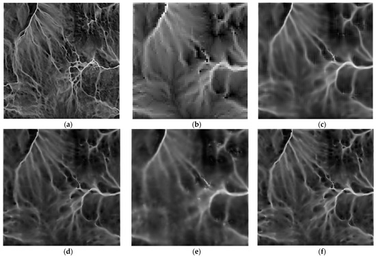
Figure 4.
TWI calculated from resampled DEM in Dataset 5 (5 m resolution): (a) TWI from reference DEM; (b) TWI from “no resampling” 20 m DEM; (c) TWI from the DEM resampled by bilinear method; (d) TWI from the DEM resampled by bi-cubic method; (e) TWI from the DEM created by Kriging interpolation method; and (f) TWI from DEM generated by the HNN downscaling approach.
Due to the larger size of the pixels, the image for “no resampling” TWI is pixelated. Some details of the linear features that present high values of TWI, which correlate to high flow accumulation, are blurred, distorted, and pixelated. Visual comparison of the images shows an improvement in details of these features as in Figure 4c–f, representing the resulting TWI of bilinear, bi-cubic, Kriging, and HNN downscaled DEMs, respectively. Although the level of detail of TWI is still significantly lower than that of the reference image, some specific features in TWI images obtained from resampled DEMs, particularly those from bi-cubic and HNN downscaled DEMs, exhibit less blurring and pixelation than those from the non-resampled DEM. Among these resampling approaches, both bi-cubic and HNN show comparable performance, with HNN slightly outperforming bi-cubic. In contrast, the Kriging and bilinear methods perform significantly worse than the other two.
3.6. Relationship between the Accuracy Improvement of Resampled Digital Elevation Model and Topographic Factors
By comparing the improvement in accuracy of digital elevation models (DEMs) and topographic factors, it is apparent that the accuracy improvement of the first derivatives of DEM correlates with the accuracy of DEM. As demonstrated in Table 2, resampling techniques such as bi-cubic and HNN downscaling significantly reduced the RMSE of DEM. The evidence of that is these techniques enhanced the accuracy of DEMs in all five experiment datasets. Similarly, the accuracy of the first derivative factors, such as slope and aspect, improved substantially (Table 3 and Table 4). The RMSE and other statistical measures confirm that the accuracy enhancement of DEM led to an overall improvement in slope and aspect accuracy for all five datasets.
The investigation of the relationship between the accuracy improvement of digital elevation models (DEMs) and resulting second derivatives of curvatures and topographic wetness index did not show the correlation as that of the first derivatives. The statistics reveal that the accuracy improvement of resampled DEMs does not necessarily translate into the improvement in the accuracy of second derivatives for all types of DEMs. The improvement of DEMs only impacted low-to-medium resolutions, as demonstrated by the reduction in RMSE of the curvatures and TWI in Dataset 1 (90 m to 30 m) and Dataset 2 (60 m to 20 m). However, while the accuracy improvement of DEMs led to enhanced accuracy of plan and profile curvatures and topographic wetness index in two medium-to-high resolution cases, the RMSE of these derivatives increased in other cases. Thus, it is not advisable to use resampled DEMs to calculate these second derivatives for medium-to-high resolution cases, such as downscaling from 20 m to 5 m and 30 m to 10 m.
4. Conclusions
This research evaluates and compares the effects of resampling and downscaling the digital elevation model (DEM) and the five associated morphometric factors (slope, aspect, plan curvature, profile curvature, and topographic wetness index) using four interpolation methods, namely the Hopfield Neural Network (HNN), Bilinear, Bicubic, and Kriging methods. From the results of the experiment, it is possible to draw the conclusions as follows:
- Both bi-cubic and HNN downscaling outperform Kriging and bilinear resampling techniques. Specifically, the results suggest that HNN has a slight advantage over bi-cubic resampling.
- Resampling approaches applied to DEMs have demonstrated their effectiveness in enhancing the quality of their derived derivatives, with remarkable improvements observed in the first derivatives of slope and aspect, as indicated by the reduction in RMSEs and other statistical metrics.
- Resampling techniques from low to medium resolutions have proven valuable in enhancing the accuracy of second derivatives, including plan and profile curvatures and the TWI. The resampling and downscaling approaches have shown their capability to improve the accuracy of these topographic factors, as evident in the results. However, the improvement of DEM’s accuracy, as indicated by reduced RMSEs, does not translate into enhancing accuracy for the second group of medium-to-high-resolution DEM data. Therefore, further investigations are required to understand the impacts of resampling and downscaling of DEMs from medium to high resolutions.
- Future investigations should be undertaken to explore the impacts of the other downscaling methods, such as deep learning for downscaling, which has been proven to positively impact to DEM’s accuracy enhancement recently. In addition, the direct downscaling of topographic factors, especially of the second derivatives such as curvatures and TWI, from lower resolution to higher resolution, also should be evaluated to find the best solutions for enhancing their accuracy.
Author Contributions
Conceptualization, N.Q.M. and P.Q.K.; methodology, N.Q.M.; software, N.T.T.H.; validation, L.P.H. and D.T.B.; formal analysis, P.Q.K.; data curation, P.Q.K.; writing—original draft preparation, D.T.B. and N.Q.M.; writing—review and editing, L.P.H. and D.T.B.; visualization, N.T.T.H. All authors have read and agreed to the published version of the manuscript.
Funding
This research was funded by the Ministry of Education and Training of Vietnam, grant number B2021-MDA-04.
Data Availability Statement
Not applicable.
Acknowledgments
The research presented in this paper results from the project title B2021-MDA-04, funded by the Ministry of Education and Training. The authors would like to express their sincere gratitude to the Ministry of Education and Training and the University of Mining and Geology for providing the necessary support and resources to complete this research.
Conflicts of Interest
The authors declare no conflict of interest.
References
- Erdogan, S. A comparision of interpolation methods for producing digital elevation models at the field scale. Earth Surf. Process. Landf. 2009, 34, 366–376. [Google Scholar] [CrossRef]
- Yang, L.; Meng, X.; Zhang, X. SRTM DEM and its application advances. Int. J. Remote Sens. 2011, 32, 3875–3896. [Google Scholar] [CrossRef]
- Mesa-Mingorance, J.L.; Ariza-López, F.J. Accuracy assessment of digital elevation models (DEMs): A critical review of practices of the past three decades. Remote Sens. 2020, 12, 2630. [Google Scholar] [CrossRef]
- Brock, J.; Schratz, P.; Petschko, H.; Muenchow, J.; Micu, M.; Brenning, A. The performance of landslide susceptibility models critically depends on the quality of digital elevation models. Geomat. Nat. Hazards Risk 2020, 11, 1075–1092. [Google Scholar] [CrossRef]
- Moretto, S.; Bozzano, F.; Mazzanti, P. The role of satellite InSAR for landslide forecasting: Limitations and openings. Remote Sens. 2021, 13, 3735. [Google Scholar] [CrossRef]
- Kumar, N.; Singh, S.K. Soil erosion assessment using earth observation data in a trans-boundary river basin. Nat. Hazards 2021, 107, 1–34. [Google Scholar] [CrossRef]
- Chidi, C.L.; Zhao, W.; Chaudhary, S.; Xiong, D.; Wu, Y. Sensitivity assessment of spatial resolution difference in DEM for soil erosion estimation based on UAV observations: An experiment on agriculture terraces in the middle hill of Nepal. ISPRS Int. J. Geo-Inf. 2021, 10, 28. [Google Scholar] [CrossRef]
- Rocha, J.; Duarte, A.; Silva, M.; Fabres, S.; Vasques, J.; Revilla-Romero, B.; Quintela, A. The importance of high resolution digital elevation models for improved hydrological simulations of a mediterranean forested catchment. Remote Sens. 2020, 12, 3287. [Google Scholar] [CrossRef]
- Muthusamy, M.; Casado, M.R.; Butler, D.; Leinster, P. Understanding the effects of Digital Elevation Model resolution in urban fluvial flood modelling. J. Hydrol. 2021, 596, 126088. [Google Scholar] [CrossRef]
- Wassmann, R.; Hien, N.X.; Hoanh, C.T.; Tuong, T.P. Sea Level Rise Affecting the Vietnamese Mekong Delta: Water Elevation in the Flood Season and Implications for Rice Production. Clim. Chang. 2004, 66, 89–107. [Google Scholar] [CrossRef]
- Minderhoud, P.; Coumou, L.; Erkens, G.; Middelkoop, H.; Stouthamer, E. Mekong delta much lower than previously assumed in sea-level rise impact assessments. Nat. Commun. 2019, 10, 3847. [Google Scholar] [CrossRef] [PubMed]
- Carlà, T.; Intrieri, E.; Di Traglia, F.; Nolesini, T.; Gigli, G.; Casagli, N. Guidelines on the use of inverse velocity method as a tool for setting alarm thresholds and forecasting landslides and structure collapses. Landslides 2017, 14, 517–534. [Google Scholar] [CrossRef]
- Dou, J.; Yunus, A.P.; Tien Bui, D.; Sahana, M.; Chen, C.-W.; Zhu, Z.; Wang, W.; Pham, B.T. Evaluating GIS-based multiple statistical models and data mining for earthquake and rainfall-induced landslide susceptibility using the LiDAR DEM. Remote Sens. 2019, 11, 638. [Google Scholar] [CrossRef]
- Mahalingam, R.; Olsen, M.J. Evaluation of the influence of source and spatial resolution of DEMs on derivative products used in landslide mapping. Geomat. Nat. Hazards Risk 2016, 7, 1835–1855. [Google Scholar] [CrossRef]
- Mukherjee, S.; Joshi, P.K.; Mukherjee, S.; Ghosh, A.; Garg, R.; Mukhopadhyay, A. Evaluation of vertical accuracy of open source Digital Elevation Model (DEM). Int. J. Appl. Earth Obs. Geoinf. 2013, 21, 205–217. [Google Scholar] [CrossRef]
- Kršák, B.; Blišťan, P.; Pauliková, A.; Puškárová, P.; Kovanič, Ľ.m.; Palková, J.; Zelizňaková, V. Use of low-cost UAV photogrammetry to analyze the accuracy of a digital elevation model in a case study. Measurement 2016, 91, 276–287. [Google Scholar] [CrossRef]
- Bolkas, D. Assessment of GCP number and separation distance for small UAS surveys with and without GNSS-PPK positioning. J. Surv. Eng. 2019, 145, 04019007. [Google Scholar] [CrossRef]
- Rogers, S.R.; Manning, I.; Livingstone, W. Comparing the spatial accuracy of digital surface models from four unoccupied aerial systems: Photogrammetry versus LiDAR. Remote Sens. 2020, 12, 2806. [Google Scholar] [CrossRef]
- Rees, W.G. The accuracy of digital elevation models interpolated to higher resolutions. Int. J. Remote Sens. 2000, 21, 7–20. [Google Scholar] [CrossRef]
- Nguyen, Q.M.; Nguyen, T.T.H.; La, P.H.; Lewis, H.G.; Atkinson, P.M. Downscaling gridded DEMs using the hopfield neural network. IEEE J. Sel. Top. Appl. Earth Obs. Remote Sens. 2019, 12, 4426–4437. [Google Scholar] [CrossRef]
- Grohmann, C.H.; Steiner, S.S. SRTM resample with short distance-low nugget kriging. Int. J. Geogr. Inf. Sci. 2008, 22, 895–906. [Google Scholar] [CrossRef]
- Jiao, D.; Wang, D.; Lv, H.; Peng, Y. Super-resolution reconstruction of a digital elevation model based on a deep residual network. Open Geosci. 2020, 12, 1369–1382. [Google Scholar] [CrossRef]
- Zhang, R.; Bian, S.; Li, H. RSPCN: Super-resolution of digital elevation model based on recursive sub-pixel convolutional neural networks. ISPRS Int. J. Geo-Inf. 2021, 10, 501. [Google Scholar] [CrossRef]
- Shin, D.; Spittle, S. LoGSRN: Deep super resolution network for digital elevation model. In Proceedings of the 2019 IEEE International Conference on Systems, Man and Cybernetics (SMC), Bari, Italy, 6–9 October 2019; pp. 3060–3065. [Google Scholar]
- Lin, X.; Zhang, Q.; Wang, H.; Yao, C.; Chen, C.; Cheng, L.; Li, Z. A DEM Super-Resolution Reconstruction Network Combining Internal and External Learning. Remote Sens. 2022, 14, 2181. [Google Scholar] [CrossRef]
- Zhang, Y.; Yu, W. Comparison of DEM Super-Resolution Methods Based on Interpolation and Neural Networks. Sensors 2022, 22, 745. [Google Scholar] [CrossRef]
- Hopfield, J.J. Neurons with graded response have collective computational properties like those of two-state neurons. Proc. Natl. Acad. Sci. USA 1984, 81, 3088–3092. [Google Scholar] [CrossRef]
- Bovik, A.C. Chapter 3—Basic Gray Level Image Processing. In The Essential Guide to Image Processing; Bovik, A., Ed.; Academic Press: Boston, MA, USA, 2009; pp. 43–68. [Google Scholar] [CrossRef]
- Chen, Y.; Yang, R.; Zhao, N.; Zhu, W.; Huang, Y.; Zhang, R.; Chen, X.; Liu, J.; Liu, W.; Zuo, Z. Concentration Quantification of Oil Samples by Three-Dimensional Concentration-Emission Matrix (CEM) Spectroscopy. Appl. Sci. 2020, 10, 315. [Google Scholar] [CrossRef]
- Bivand, R.S.; Pebesma, E.J.; Gomez-Rubio, V.; Pebesma, E.J. Applied Spatial Data Analysis with R; Springer: Berlin/Heidelberg, Germany, 2008; Volume 747248717. [Google Scholar]
- Dunn, M.; Hickey, R. The effect of slope algorithms on slope estimates within a GIS. Cartography 1998, 27, 9–15. [Google Scholar] [CrossRef]
- Jones, K.H. A comparison of algorithms used to compute hill slope as a property of the DEM. Comput. Geosci. 1998, 24, 315–323. [Google Scholar] [CrossRef]
- Pham, B.T.; Tien Bui, D.; Prakash, I. Bagging based support vector machines for spatial prediction of landslides. Environ. Earth Sci. 2018, 77, 1–17. [Google Scholar]
- Deng, Y.; Wilson, J.P.; Bauer, B. DEM resolution dependencies of terrain attributes across a landscape. Int. J. Geogr. Inf. Sci. 2007, 21, 187–213. [Google Scholar] [CrossRef]
- Kienzle, S. The effect of DEM raster resolution on first order, second order and compound terrain derivatives. Trans. GIS 2004, 8, 83–111. [Google Scholar] [CrossRef]
- Zevenbergen, L.W.; Thorne, C.R. Quantitative analysis of land surface topography. Earth Surf. Process. Landf. 1987, 12, 47–56. [Google Scholar] [CrossRef]
- Beven, K.J.; Kirkby, M.J. A physically based, variable contributing area model of basin hydrology/Un modèle à base physique de zone d’appel variable de l’hydrologie du bassin versant. Hydrol. Sci. Bull. 1979, 24, 43–69. [Google Scholar] [CrossRef]
- Güntner, A.; Seibert, J.; Uhlenbrook, S. Modeling spatial patterns of saturated areas: An evaluation of different terrain indices. Water Resour. Res. 2004, 40, 1–19. [Google Scholar] [CrossRef]
- Zhou, Q.; Liu, X. Error Analysis on Grid-Based Slope and Aspect Algorithms. Photogramm. Eng. Remote Sens. 2004, 70, 957–962. [Google Scholar] [CrossRef]


Disclaimer/Publisher’s Note: The statements, opinions and data contained in all publications are solely those of the individual author(s) and contributor(s) and not of MDPI and/or the editor(s). MDPI and/or the editor(s) disclaim responsibility for any injury to people or property resulting from any ideas, methods, instructions or products referred to in the content. |
© 2024 by the authors. Licensee MDPI, Basel, Switzerland. This article is an open access article distributed under the terms and conditions of the Creative Commons Attribution (CC BY) license (https://creativecommons.org/licenses/by/4.0/).